Anderson localization from classical trajectories

Abstract

We show that Anderson localization in quasi-one dimensional conductors with ballistic electron dynamics, such as an array of ballistic chaotic cavities connected via ballistic contacts, can be understood in terms of classical electron trajectories only. At large length scales, an exponential proliferation of trajectories of nearly identical classical action generates an abundance of interference terms, which eventually leads to a suppression of transport coefficients. We quantitatively describe this mechanism in two different ways: the explicit description of transition probabilities in terms of interfering trajectories, and an hierarchical integration over fluctuations in the classical phase space of the array cavities.

I Introduction

The interplay of quantum phase coherence and repeated random scattering is at the origin of many effects in mesoscopic physics.Akkermans et al. (1995); Imry (2002) These effects include weak localization and universal conductance fluctuations, both of which are small but fundamental corrections with respect to the conductance obtained from Drude-Boltzmann theory. They culminate in Anderson localization, the phenomenon that the resistance of a one or two-dimensional electron gas grows exponentially with system size if the system size is sufficiently large.Anderson (1958); Abrahams et al. (1979)

Originally, Anderson localization and other mesoscopic effects were discovered in the context of disordered metals, in which electrons scatter off impurities with a size comparable to their wavelength. Theoretically, quantum effects in disordered metals are described using the ‘disorder average’ which deals with an ensemble of macroscopically equivalent but microscopically different impurity configurations. The presence of impurities is not essential for the existence of quantum effects, however. The same effects, with the same statistical properties, have been found to appear if the electron motion is ballistic and chaotic, the only source of scattering of electrons being specular reflection off the sample boundaries.Stone (1995); Nakamura and Harayama (2004); foot1 Besides being of theoretical interest for understanding the quantum properties of systems with chaotic classical dynamics,Haake (1991) the case of ballistic electron motion is relevant experimentally for very clean artificially structured two-dimensional electron gases in semiconductor heterostructures, such as quantum dots or antidot lattices.Kouwenhoven et al. (1997); Roukes and Scherer (1989); Ensslin and Petroff (1990)

Unlike disordered metals, in which impurities scatter diffractively, electrons in ballistic conductors have a well-defined classical dynamics. Many quantum properties of ballistic conductors with chaotic classical dynamics can be understood in terms of classical mechanics by making use of well-chosen semiclassical methods.Haake (1991); Nakamura and Harayama (2004) A well-known example is the Gutzwiller trace formula, which relates the density of states to properties of periodic orbits of the classical dynamics.Gutzwiller (1990) For the conductance $G$ and its quantum corrections, there is a variant of Gutzwiller’s formula, which expresses $G$ as a double sum over classical trajectories $\alpha$ and $\beta$ connecting the source and drain contacts,Jalabert et al. (1990); Stone (1995)

$$G=\frac{1}{2\pi\hbar}\int dpdq\,A_{\alpha}A_{\beta}e^{i({\cal S}_{\alpha}-{\cal S}_{\beta})/\hbar}.$$ (1)

Upon entrance and exit, the trajectories $\alpha$ and $\beta$ have the same transverse momenta $p$ and $q$, respectively, but the position at which they enter or exit the sample may be different. Further, $A_{\alpha,\beta}$ and ${\cal S}_{\alpha,\beta}$ are the so-called “stability amplitude” and the classical action of the trajectories.

With Eq. (1) as a starting point, the conductance, including its quantum corrections, can be calculated solely from knowledge of classical trajectories. Quantum effects have been linked to the existence of families of classical trajectories that only differ near ‘small-angle encounters’ of the trajectory with itself.Sieber and Richter (2001); Sieber (2002); Richter and Sieber (2002); Müller et al. (2007a); foot2 This semiclassical approach has been very successful explaining quantum effects in the ‘perturbative regime’ in which quantum interference provides a small correction to the classical mechanics.Sieber and Richter (2001); Sieber (2002); Richter and Sieber (2002); Müller et al. (2004, 2005); Heusler et al. (2006a); Whitney and Jacquod (2006); Brouwer and Rahav (2006a); Müller et al. (2007a) Weak localization and universal conductance fluctuations are examples of such perturbative quantum effects. Recently, Heusler et al. showed that it is also possible to understand quantum effects in terms of classical trajectories outside the perturbative regime. They considered the spectral form factor $K(t)$ of a ballistic cavity, the Fourier transform of the two-point correlation function of the density of states. A direct semiclassical evaluation of $K(t)$ using Gutzwiller’s trace formula was known to be possible in the perturbative regime $t<t_{\rm H}$ only, where the Heisenberg time $t_{\rm H}=h/\Delta$, $\Delta$ being the cavity’s mean level spacing.Berry (1985); Aleiner and Larkin (1997); Sieber and Richter (2001); Sieber (2002); Müller et al. (2004, 2005) Motivated by the field-theoretical formulation of the problem, Heusler et al. used a different way to express $K(t)$ in terms of periodic orbits that allowed them to calculate $K(t)$ for all times.Heusler et al. (2006b)

In this communication, we consider Anderson localization for ballistic electron gases, and show that it, too, can be understood in terms of interference of classical trajectories, with Eq. (1) as a starting point. Examples of systems that may exhibit such ‘ballistic Anderson localization’ are antidot lattices or arrays of chaotic cavities. Although it is generally accepted that Anderson localization exists irrespective of the details of the microscopic electronic dynamics,foot3 the similarity of the phenomena for ballistic and disordered electron systems should not obscure the vastly different starting points of the theories for the two cases. This difference not only pertains to the microscopic dynamics (classical-deterministic vs. quantum-probabilistic), but also to the statistical assumptions of the theory. Unlike theories of quantum transport in disordered metals, semiclassical theories of ballistic conductors are intended to describe one specific system.Haake (1991) Fluctuations appear solely from variations of the Fermi energy; no changes in the classical dynamics are invoked.

For disordered metals, Anderson localization is most prominent for a quasi-one dimensional geometry, with sample length $L$ much larger than the sample width $W$. For quasi-one dimensional samples, a full theory of transport in the localized regime was developed by DorokhovDorokhov (1982) and Mello, Pereyra, and Kumar,Mello et al. (1988) using a stochastic approach, and by Efetov and Larkin,Efetov (1983); Efetov and Larkin (1983) using a field-theoretic approach. Our theory of ballistic Anderson localization closely follows these approaches. The fact that the semiclassical theory for ballistic electrons follows the corresponding quantum mechanical theory for disordered metals is not special to the present case. It is also typical of the trajectory-based semiclassical theories in the perturbative regime, which have a structure that resembles the diagrammatic perturbation theory of quantum corrections in disordered metals.Sieber and Richter (2001); Sieber (2002); Richter and Sieber (2002)

In addition to the ballistic electron gases considered here, Anderson localization also occurs in certain dynamic systems with a periodic time-dependent Hamiltonian, such as the kicked rotor.Haake (1991) Classically, the dynamics of the kicked rotor is chaotic, with a momentum that changes diffusively under the influence of the periodic kicks. Quantum mechanically, it exhibits ‘dynamic localization’, Anderson localization in momentum space rather than in real space.Fishman et al. (1982) The phenomenology of dynamic localization is equal to that of Anderson localization in disordered metals. This is confirmed by extensive numerical simulations,Casati et al. (1979); Shepelyansky (1986) as well as a field theoretical analysis of the problem.Altland and Zirnbauer (1996a)

The trajectory-based theory of ballistic Anderson localization that we report here is constructed for a specific system, an array of chaotic cavities. A schematic drawing of such an array is shown in Fig. 1. We use this model system because the trajectory-based theory of transport through a single chaotic cavity is well established in the literature.Jalabert et al. (1990); Baranger et al. (1993a, b); Richter and Sieber (2002); Heusler et al. (2006a); Müller et al. (2007a); Brouwer and Rahav (2006a) Arrays of cavities have been used as a starting point for a field-theoretic description of Anderson localization using random matrix theory,Mirlin et al. (1994); Brouwer and Frahm (1996) but not with Dorokhov’s method. In Sec. II we show how Dorokhov’s theory can be adapted to this system if the cavities are disordered and random matrix theory can be used to describe transport through a single cavity. In Sec. III we summarize the basic elements of the trajectory-based semiclassical formalism. This formalism is used to construct the trajectory-based semiclassical theory of ballistic localization in Sec. IV. In section V we approach the localization phenomenon from a different perspective. We describe the array in terms of a nonlinear $\sigma$-model whose perturbative (‘diagrammatic’) evaluation generates structures of paired Feynman amplitudes similar to those appearing in the native semiclassical approach. Alternatively, the dynamical structure of the theory can be analyzed to identify and successively eliminate hierarchies of different types of dynamical fluctuations in the system. In this way we obtain an effective low energy theory which turns out to be equivalent to the nonlinear $\sigma$-model of diffusive quantum wires; the latter model is known to predict exponential localization at large length scales. We conclude in Sec. VI.

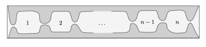
Figure 1: (Color online) Schematic drawing of an array of $n$ chaotic cavities. The cavities are connected via ballistic contacts with dimensionless conductance $g_{\rm c}$. The semiclassical theory requires the limit $g_{\rm c}\to\infty$ at a fixed ratio $n/g_{\rm c}$.

II Array of disordered cavities

We now describe how Dorokhov’s approach can be used to describe Anderson localization in an array of disordered cavities or quantum dots. We take the disorder in each cavity to be weak (cavity size much smaller than the localization length), so that transport through a single cavity is described by random matrix theory.Beenakker (1997)

A schematic drawing of the array of cavities is shown in Fig. 1. The cavities are connected via ballistic contacts with dimensionless conductance $g_{\rm c}$. Since we want to compare with a semiclassical theory for an array of ballistic cavities, we require $g_{\rm c}\gg 1$. Localization takes place if the conductance of the array is of order unity. This condition is met if the number $n$ of cavities in the array is comparable to $g_{\rm c}$. Hence, in the calculations below we take the limit $g_{\rm c}\to\infty$ while keeping the ratio $n/g_{\rm c}$ fixed. The same limit is taken in the field theoretical description of localization,Efetov (1983); Efetov and Larkin (1983); Zirnbauer (1992); Mirlin et al. (1994); Brouwer and Frahm (1996) where it is known as the “thick wire limit”.

The transport properties of the array of cavities are encoded in its scattering matrix $S^{\rm q}(n)$. (The superscript “q” is used to distinguish the quantum mechanical scattering matrix from its semiclassical counterpart to be introduced in Sec. III.) The matrix indices of $S^{\rm q}(n)$ represent the two contacts $i=1,2$ at the far left and right of the array and the transverse modes in each contact, $|p_{\perp,i}|=\pm\pi\hbar n_{i}/W$, $n_{i}=1,2,\ldots,N$, where $N=g_{\rm c}$ is the number of channels in contact $i$, $i=1,2$. The matrix $S^{\rm q}(n)$ is a random quantity because it depends on the Fermi energy and on the precise disorder configuration in each cavity. Following the approach of Dorokhov, Mello, Pereyra, and Kumar,Dorokhov (1982); Mello et al. (1988) we consider the hermitian matrix

$${\cal T}^{\rm q}(n)=S_{12}^{\rm q}(n)S_{12}^{{\rm q}\dagger}(n),$$ (2)

and calculate its statistical distribution by expressing ${\cal T}^{\rm q}(n)$ in terms of ${\cal T}^{\rm q}(n-1)$ and proceeding recursively. The matrix ${\cal T}^{\rm q}$ is related to the dimensionless conductance $g(n)$ of the array through the Landauer formula,

$$g(n)=\mbox{tr}\,{\cal T}^{\rm q}(n).$$ (3)

Taking the scattering matrix of each individual cavity from the circular ensemble of random matrix theory,Beenakker (1997) one then finds that the recursion relation for ${\cal T}^{\rm q}$ takes the form

$$\delta{\cal T}^{\rm q} = {\cal T}^{\rm q}(n)-{\cal T}^{\rm q}(n-1)$$ (4)

$$= -\frac{1}{g_{\rm c}}{\cal T}^{\rm q}(n-1)\mbox{tr}\,{\cal T}^{\rm q}(n-1)-\frac{1}{g_{\rm c}}\delta_{\beta,1}{\cal T}^{\rm q}(n-1)^{2}$$

$$\mbox{}+{\cal X}^{\rm q}(n)+{\cal O}(g_{\rm c}^{-3/2}),$$

where the hermitian matrix ${\cal X}$ is a random (noise) term with a Gaussian distribution,

$$\langle{\cal X}^{\rm q}(n)_{ij}\rangle_{n} = 0,$$ (5)

$$\langle{\cal X}^{\rm q}(n)_{ij}{\cal X}^{\rm q}(n)_{kl}\rangle_{n} = \frac{1}{g_{\rm c}}{\cal T}^{\rm q}(n-1)_{il}{\cal F}^{\rm q}_{kj}$$

$$\mbox{}+\frac{1}{g_{\rm c}}{\cal T}^{\rm q}(n-1)_{kj}{\cal F}^{\rm Q}_{il}$$

$$\mbox{}+\frac{2}{g_{\rm c}}\delta_{\beta,1}{\cal G}^{\rm q}_{ij}{\cal G}^{{\rm q}*}_{kl},$$

where ${\cal F}^{\rm q}={\cal T}^{\rm q}(1-{\cal T}^{\rm q})$, $\beta=1$ or $2$ in the presence or absence of time-reversal symmetry, respectively, and

$${\cal G}^{\rm q}=S_{12}^{\rm q}S_{22}^{{\rm q}\dagger}S_{21}^{\rm q}.$$ (6)

The averaging brackets $\langle\ldots\rangle_{n}$ denote an average with respect to the disorder configuration in the $n$th cavity only.

In the limit $g_{\rm c}\to\infty$ while keeping $n/g_{\rm c}$ fixed, the stochastic recursion relation (4) can be mapped to the Dorokhov-Mello-Pereyra-Kumar (DMPK) equation, which is a stochastic differential equation for the eigenvalues of ${\cal T}^{\rm q}$.Dorokhov (1982); Mello et al. (1988); Beenakker (1997); foot4 The solution of the DMPK equation is known,Beenakker (1997) which completes the theory of localization for an array of disordered cavities.

Alternatively, the stochastic recursion relation (4) can be used to generate a coupled set of recursion relations for the disorder averages of the moments of ${\cal T}(n)$,

$$\delta\left\langle\prod_{m=1}^{n}T_{i_{m}}\right\rangle = \left\langle\prod_{m=1}^{n}T_{i_{m}}(n)\right\rangle-\left\langle\prod_{m=1}^{n}T_{i_{m}}(n-1)\right\rangle$$ (7)

$$= -\frac{1}{g_{\rm c}}\delta_{\beta,1}\sum_{k=1}^{n}i_{k}\left\langle T_{i_{k}+1}\prod_{{m=1}\atop{m\neq k}}^{n}T_{i_{m}}\right\rangle-\frac{1}{g_{\rm c}}\left(\sum_{k=1}^{n}i_{k}\right)\left\langle T_{1}\prod_{m=1}^{n}T_{i_{m}}\right\rangle$$

$$\mbox{}+\frac{1}{g_{\rm c}}\sum_{k=1}^{n}\sum_{j=1}^{i_{k}-1}i_{k}\left\langle(T_{j}(T_{i_{k}-j}-T_{i_{k}-j+1}))\prod_{{m=1\atop m\neq k}}^{n}T_{i_{m}}\right\rangle$$

$$\mbox{}+\frac{4}{\beta g_{\rm c}}\sum_{k=1}^{n}\sum_{l=1}^{k-1}i_{k}i_{l}\left\langle(T_{i_{k}+i_{l}}-T_{i_{k}+i_{l}+1})\prod_{{m=1\atop m\neq k,l}}^{n}T_{i_{m}}\right\rangle+{\cal O}(g_{\rm c}^{-2}),$$

with

$$T_{m}=\mbox{tr}\,({\cal T}^{\rm q})^{m}.$$ (8)

(The argument $n-1$ is suppressed on the right hand side of the second equality.) The average in Eq. (7) is the full disorder average, applied to all cavities in the array. Taking the limit $g_{\rm c}\to\infty$ at fixed $n/g_{\rm c}$, Eq. (7) is mapped to a coupled set of differential equations for the moments of ${\cal T}^{\rm q}$ which is identical to the corresponding set of differential equations for a disordered wire.Tartakovski (1995); Brouwer (1998) A subset of these equations can be resummed into a partial differential equation for the generating function $F_{\beta}$, withRejaei (1996); Brouwer and Frahm (1996)

$$F_{1} = \left\langle\det\prod_{\pm}\left(\frac{2+(\cos(\theta_{3})-1){\cal T}^{\rm q}}{2+(\cosh(\theta_{1}\pm\theta_{2})-1){\cal T}^{\rm q}}\right)^{1/2}\right\rangle,$$

$$F_{2} = \left\langle\det\left(\frac{2+(\cos(\theta_{3})-1){\cal T}^{\rm q}}{2+(\cosh(\theta_{1})-1){\cal T}^{\rm q}}\right)\right\rangle.$$ (9)

As shown in Refs. Rejaei, 1996; Brouwer and Frahm, 1996, the resulting theory of localization in quasi-one dimension is formally equivalent to that obtained from the one-dimensional nonlinear sigma model.Efetov (1983); Efetov and Larkin (1983); Zirnbauer (1992); Mirlin et al. (1994)

III Semiclassical formalism

The central object in the trajectory-based semiclassical theory of localization in an array of ballistic chaotic cavities is a semiclassical representation of the scattering matrix $S^{\rm q}$. In the semiclassical representation, the discrete transverse momenta become continuous variables, so that the scattering matrix $S^{\rm q}$ becomes a ‘scattering kernel’ $S_{ij}(p^{\prime},p)$. Following standard semiclassical approximations, this scattering kernel is then represented as a sum over classical trajectories $\alpha$ connecting contact $j$ to contact $i$,Jalabert et al. (1990); Stone (1995)

$$S_{ij}(p^{\prime},p)=\frac{1}{\sqrt{2\pi\hbar}}\sum_{\alpha}A_{\alpha}e^{i{\cal S}_{\alpha}/\hbar},$$ (10)

such that the transverse momentum of $\alpha$ upon entrance and exit equals $p$ and $p^{\prime}$, respectively. Further, ${\cal S}_{\alpha}$ is the classical action of $\alpha$, and $A_{\alpha}$ the stability amplitude,

$$A=\left|\frac{\partial p^{\prime}}{\partial q}\right|^{-1/2},$$ (11)

where $q$ is the transverse position upon entrance into the sample. Maslov indices and other additional phase shifts are included in ${\cal S}_{\alpha}$. Because the transverse modes in the quantum mechanical formulation are linked to the absolute value of the transverse momentum, not to the transverse momentum itself, the semiclassical counterpart of the products $S_{ij}S_{kj}^{\dagger}$ and $S_{jk}^{\dagger}S_{ji}$ consist of two contributions: one in which transverse momenta in contact $j$ are equal and one in which the transverse momenta are opposite,

$$[S_{ij}^{\vphantom{M}}S_{kj}^{\dagger}](p^{\prime},p) = \sum_{\pm}\int_{-p_{F}}^{p_{F}}\frac{dp^{\prime\prime}}{2\pi\hbar}S_{ij}^{\vphantom{M}}(p^{\prime},p^{\prime\prime})S_{kj}^{\dagger}(p,\pm p^{\prime\prime}),$$

$$[S_{jk}^{\dagger}S_{ji}^{\vphantom{M}}](p^{\prime},p) = \sum_{\pm}\int_{-p_{F}}^{p_{F}}\frac{dp^{\prime\prime}}{2\pi\hbar}S_{jk}^{\dagger}(\pm p^{\prime\prime},p^{\prime})S_{ji}^{\vphantom{M}}(p^{\prime\prime},p),$$

Together, Eqs. (10) and (LABEL:eq:Sproduct) specify how products of the quantum-mechanical scattering matrix and its hermitian conjugate are expressed in terms of classical trajectories. [The “$-$” terms in the summations were omitted from the semiclassical expression for the conductance, Eq. (1) above.]

For a theory of Anderson localization, we are interested in the trace of a product of alternating factors $S$ and $S^{\dagger}$ or in the product of such traces. Using the semiclassical representation (10), a polynomial function $F(S,S^{\dagger})$ that involves the alternating product of $n$ factors $S$ and $n$ factors $S^{\dagger}$ is written as a summation over $2n$ classical trajectories $\alpha_{1},\ldots,\alpha_{n}$ and $\beta_{1},\ldots,\beta_{n}$, one trajectory for each factor $S$ or $S^{\dagger}$, respectively. Each configuration of classical trajectories is weighed by a phase factor $\exp(i\Delta{\cal S}/\hbar)$ with

$$\Delta{\cal S}=\sum_{i=1}^{n}{\cal S}_{\alpha_{i}}-\sum_{i=1}^{n}{\cal S}_{\beta_{i}}.$$ (13)

Building on work by Richter and Sieber,Sieber and Richter (2001); Sieber (2002); Richter and Sieber (2002) Haake and coworkers have identified a hierarchy of families of classical trajectories $\alpha_{1}$,…,$\beta_{n}$ that contribute to the average $\langle F\rangle$,Müller et al. (2004, 2005); Heusler et al. (2006a); Müller et al. (2007a) where the average is taken with respect to variations of the Fermi energy while keeping the classical dynamics (i.e., the shape of the cavities) fixed. Their identification is based on the recognition that families of trajectories contribute to $\langle F\rangle$ only if their total action difference $\Delta{\cal S}$ is of order $\hbar$ systematically, which happens only if the trajectories $\alpha_{i}$ are piecewise and pairwise identical to the trajectories $\beta_{j}$, $i,j=1,\ldots,n$, up to classical phase space distances of order ${\hbar}^{1/2}$.Sieber and Richter (2001); Sieber (2002) Trajectories that are separated by larger phase space distances have typical action differences $\Delta{\cal S}$ that are parametrically larger than $\hbar$, so that their contribution vanishes upon taking the average.

The simplest choice for a family of trajectories for which $\Delta{\cal S}$ is of order $\hbar$ systematically is if each trajectory $\alpha_{i}$ equals another trajectory $\beta_{j}$ for the full length of the trajectory. Calculating $\langle F\rangle$ from the contribution from such families of trajectories only is known as the “diagonal approximation”.Jalabert et al. (1990); Baranger et al. (1993a, b) Nontrivial families of trajectories emerge from the possibility of small-angle encounters between trajectories, at which more than two trajectories are within a phase space distance $\sim\hbar^{1/2}$.Aleiner and Larkin (1996) At such small-angle encounters, the pairing between the $\alpha_{i}$ and $\beta_{j}$ can be changed — so that now trajectories need to be piecewise identical only. The duration of a small-angle encounter is the “Ehrenfest time” $\tau_{\rm E}=\lambda^{-1}\ln(p_{F}l/\hbar)$, where $\lambda$ is the Lyapunov exponent of the classical dynamics, $p_{F}$ the Fermi momentum, and $l$ a characteristic length scale of the classical dynamics. The fundamental action integrals corresponding to each small-angle encounter are known, Spehner (2003); Turek and Richter (2003); Müller et al. (2004, 2005) and the resulting theory takes the form of simple combinatorial rules with which any product of traces of products the scattering matrix and its hermitian conjugate can be calculated to arbitrary order in $\hbar$ from the semiclassical representation of $S$, provided that the Ehrenfest time $\tau_{\rm E}$ be much smaller than the sample’s mean dwell time $\tau_{\rm D}$.Müller et al. (2004, 2005); Heusler et al. (2006a); Müller et al. (2007a) (The case of finite $\tau_{\rm E}/\tau_{\rm D}$ is considerably more complicated, see, e.g., Refs. Whitney and Jacquod, 2006; Rahav and Brouwer, 2006; Brouwer and Rahav, 2006a; Brouwer, 2007, but not relevant for a semiclassical theory of Anderson localization.)

In the remainder of this text, we refer to a calculation of the energy-average $\langle F\rangle$ using contributions from families of trajectories thus constructed as the “trajectory-based semiclassical formalism”. Although there is no formal proof that this formalism is exact, i.e., that there are no other contributions to $\langle F\rangle$ than from families of piecewise paired classical trajectories, the formalism satisfies all known conservation rules and calculations based on trajectory-based semiclassics have been found to agree with fully quantum mechanical calculations whenever applicable.Müller et al. (2007a); Brouwer (2007) The present calculation can be viewed as another demonstration of the validity of trajectory-based semiclassics, by showing that the same formalism can serve as the starting point of a theory of localization.

While we do not need the detailed results of the trajectory-based semiclassical formalism, there are two properties of ensemble averages calculated using that formalism that are particularly relevant for our calculations below:
(i) All averages are compatible with the condition of unitarity,Müller et al. (2007a)

$$\sum_{j}[S_{ij}^{\vphantom{M}}S^{\dagger}_{kj}](p,p^{\prime}) = \sum_{j}[S^{\dagger}_{jk}S_{ji}^{\vphantom{M}}](p,p^{\prime})$$ (14)

$$= \delta_{ik}\delta(p-p^{\prime}).$$

(ii) For a product $S_{ij}^{\vphantom{M}}S^{\dagger}_{kj}$ or $S^{\dagger}_{ji}S_{jk}^{\vphantom{M}}$, the trajectory $\alpha$ of the semiclassical representation for $S$ and the trajectory $\beta$ of the semiclassical representation of $S^{\dagger}$ at contact $j$ satisfy

$$p_{\alpha}=p_{\beta},\ \ |q_{\alpha}-q_{\beta}|\lesssim\hbar/p_{F}.$$ (15)

In particular, this implies that there is no contribution from the second term in Eq. (LABEL:eq:Sproduct) for a product of two scattering kernels.Whitney and Jacquod (2006); Rahav and Brouwer (2006)

IV Array of ballistic cavities

In the perturbative regime, the semiclassical theories of quantum corrections to transport and to the density of states closely followed the corresponding theory for disordered metals. The semiclassical formalism described in the previous section was instrumental in formalizing the relation between the two types of theories. Motivated by this correspondence, we now look for the possibility to adapt the theory of localization in an array of disordered cavities [Sec. II] to the case of an array of ballistic cavities.

Thus, paraphrasing the arguments of Sec. II, the goal of our calculation will be to find the full probability distribution of the function

$${\cal T}(n;p^{\prime},p)=[S_{12}S_{12}^{\dagger}](p^{\prime},p)$$ (16)

for an array of $n$ cavities. As shown in Sec. II, there are two ways in which this can be accomplished:

1. Using a stochastic approach, in which one considers the stochastic evolution of the function ${\cal T}(n;p^{\prime},p)$ as a function of $n$, or through

2. the construction of a set of recursion relations for all moments of ${\cal T}(n)$.

In both cases, the resulting theory is formally identical to the known theories of localization in quasi-one dimension.

Although technically simpler, the stochastic approach is at odds with the goals of a semiclassical theory for ballistic localization: The goal of a theory of localization in an array of ballistic cavities is to describe an array of cavities with a fixed shape, using variations of the Fermi energy as the only source of statistical fluctuations. Since the Fermi energy is set globally, for all cavities at the same time, quantum corrections for different cavities are not independent, and a stochastic approach is ruled out a priori. A stochastic approach is possible, however, if one relaxes the goals of the theory, allowing for small variations of the shape of each cavity, or for variations of a “gate voltage” that sets the Fermi energy of each cavity independently.

Below we first describe the stochastic approach. In Sec. IV.1 we consider the case of broken time-reversal symmetry, which is technically simpler. The discussion of localization in the presence of time-reversal symmetry is given in Sec. IV.2. In Sec. IV.3 we discuss how a hierarchy of recursion relations for the moments of ${\cal T}$ can be constructed, where the average is taken with respect to variations of the Fermi energy of the entire array only.

IV.1 Stochastic approach

The stochastic approach deals with (statistical) properties of the function ${\cal T}(n)$ before averaging. Although the properties (i) and (ii) of the trajectory-based semiclassical formalism [Sec. III] are satisfied for the average of any product of traces of products alternating factors $S$ and $S^{\dagger}$ to arbitrary order in $\hbar$, they have not been shown to follow from the semiclassical scattering matrix (10) before averaging. However, since our goal is a statistical theory of the transport — the final statements of the theory will refer to averaged quantities only — we will accept these two properties on the level of the sample-specific semiclassical scattering kernel $S(n;p^{\prime},p)$ in the arguments that follow below.

Starting from Eq. (10), the kernel ${\cal T}$ is expressed as a double sum over classical trajectories $\alpha$ and $\beta$ that connect the entrance and exit contacts [Fig. 2],

$${\cal T}(p^{\prime},p)=\sum_{\alpha,\beta}\frac{A_{\alpha}A_{\beta}}{2\pi\hbar}e^{i({\cal S}_{\alpha}-{\cal S}_{\beta})/\hbar}.$$ (17)

Here $p$ and $q$ are the transverse momenta of $\alpha$ and $\beta$ upon entrance. The two trajectories have equal transverse momenta upon exit, and exit at positions a quantum uncertainty $\sim\hbar/p_{F}$ apart — see property (ii) above. Below, we express the difference $\delta{\cal T}={\cal T}(n)-{\cal T}(n-1)$ in terms of classical trajectories. We first calculate the average $\langle\delta{\cal T}\rangle_{n}$, where the average is taken with respect to variations of the Fermi energy of the $n$th cavity (or of its shape), while keeping the Fermi energy and shape of the other cavities fixed. After that, we calculate the variance of $\delta{\cal T}$ and the higher cumulants.

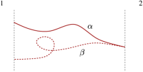
Figure 2: (Color online) Example of a pair of trajectories $\alpha$ and $\beta$ contributing to ${\cal T}(p^{\prime},p)=[S_{12}S_{12}^{\dagger}](p^{\prime},p)$. Upon entering the sample, the two trajectories have different transverse momenta $p$ and $q$, and may enter at different transverse positions. Upon exiting the sample, $\alpha$ and $\beta$ have the same transverse momentum, and exit at transverse positions a distance $\lesssim\hbar/p_{F}$ apart.

Average of $\delta{\cal T}$. When calculating the average $\langle\delta{\cal T}\rangle_{n}=\langle{\cal T}(n)\rangle_{n}-{\cal T}(n-1)$ to leading order in $1/g_{\rm c}$ in the absence of time-reversal symmetry, it will be sufficient to calculate $\langle{\cal T}(n)\rangle_{n}$ in the diagonal approximation by considering trajectories $\alpha$ and $\beta$ that are “paired” in the $n$th cavity. Note, however, that trajectories need not be paired in the first $n-1$ cavities, because no average is taken there. Each trajectory is classified by the number of times $m_{\alpha}$, $m_{\beta}$ that it enters the $n$th cavity from the $(n-1)$th cavity. Hence, for each trajectory there are $m_{\alpha}$ and $m_{\beta}$ segments in the $n$th cavity, which we label as $\alpha_{1}$, …, $\alpha_{m_{\alpha}}$ and $\beta_{1}$, …, $\beta_{m_{\beta}}$. Since trajectories are paired in the $n$th cavity, $m_{\alpha}=m_{\beta}=m$. Examples of trajectory pairs $\alpha$ and $\beta$ with $m=1$, $2$, and $3$ are shown in Fig. 3. Since trajectories need to be paired upon exit, $\alpha_{m}$ has to be paired with $\beta_{m}$. While there are $(m-1)!$ ways in which the remaining segments can be paired, we now show that the “diagonal pairing”, $\alpha_{j}$ paired with $\beta_{j}$, $j=1,\ldots,m$, gives the main contribution to $\langle\delta{\cal T}\rangle_{n}$, whereas all other pairings give contributions a factor $1/g_{\rm c}$ smaller.

Cutting the trajectories $\alpha$ and $\beta$ at the contact between the $(n-1)$st and $n$th cavity also separates the part of each trajectory that resides in the first $n-1$ cavities into $m$ segments. The first segment of each trajectory connects the entrance contact to the exit of the $(n-1)$st cavity; All other segments connect the exit contact of the $(n-1)$st cavity to itself. Since the electron dynamics in the $n$th cavity is fully ergodic, the positions and transverse momenta with which these segments cross the interface between the $(n-1)$st and $n$th cavity are fully random, without correlations between different segments. [Correlations can be ruled out down to quantum phase space distances $\sim\hbar/(p_{F}L)^{1/2}$ because the dwell time $\tau_{\rm D}\gg\tau_{\rm E}$.] Hence, these $m$ segments can be interpreted as the semiclassical representation of a product of $S_{12}$, $S_{12}^{\dagger}$, and $m-1$ factors $S_{22}$ and $S_{22}^{\dagger}$, before taking any average. Note that, although trajectories $\alpha,\beta$ that are “paired” in the $n$th cavity have a phase space distance of order $\hbar/(p_{F}L)^{1/2}$ or smaller when they enter/exit the $n$th cavity from/to the $(n-1)$st cavity, such trajectory pairs are sufficient for the semiclassical calculation of the complete kernels ${\cal T}$ because of property (ii) of Sec. III.

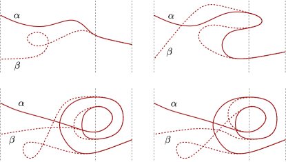
Figure 3: (Color online) Examples of trajectories $\alpha$ and $\beta$ contributing to $\langle{\cal T}(n)\rangle_{n}$, where an average is taken over the Fermi energy of the $n$th cavity only. The four panels show trajectories contributing for $m=1$ (top left), $m=2$ (top right), $m=3$ with diagonal pairing (bottom left), and $m=3$ with non-diagonal pairing (bottom right). The number $m$ counts the number of times $\alpha$ and $\beta$ enter the $n$th cavity from the $(n-1)$st cavity. The three dashed lines in each panel represent the entrance contact, the contact between the $(n-1)$st cavity and the $n$th cavity, and the exit contact (from left to right). In the $n$th cavity, the trajectories $\alpha$ and $\beta$ are piecewise equal up to quantum uncertainties.

For the diagonal pairing, the $m$ segments of $\alpha$ and $\beta$ that reside in the first $n-1$ cavities generate a particularly simple product of factors $S$ and $S^{\dagger}$, ${\cal T}(n-1)[\mbox{tr}\,{\cal R}(n-1)]^{m-1}$, where

$${\cal R}(n;p,p^{\prime})=[S_{22}(n)^{\dagger}S_{22}(n)](p,p^{\prime})$$ (18)

is the reflection coefficient for the first $n-1$ cavities, seen from the exit contact of the $(n-1)$st cavity, and

$$\mbox{tr}\,{\cal R}(n)=\int_{-p_{F}}^{p_{F}}dp\,{\cal R}(n;p,p).$$ (19)

Using the trajectory-based semiclassical formalism to evaluate the diagonal trajectory sums in the $n$th cavity,Baranger et al. (1993a, b); Richter and Sieber (2002); Heusler et al. (2006a); Müller et al. (2007a) one then easily finds that the diagonal pairing gives

$$\langle{\cal T}(n)\rangle_{n} = \sum_{m=1}^{\infty}\frac{1}{2^{m}g_{\rm c}^{m-1}}{\cal T}(n-1)[\mbox{tr}\,{\cal R}(n-1)]^{m-1}$$ (20)

$$= \frac{{\cal T}(n-1)g_{\rm c}}{2g_{\rm c}-\mbox{tr}\,{\cal R}(n-1)}.$$

Using unitarity, one has

$$\mbox{tr}\,{\cal R}(n)=g_{\rm c}-\mbox{tr}\,{\cal T}(n),$$ (21)

so that Eq. (20) can be rewritten as

$$\langle\delta{\cal T}\rangle_{n} = -\frac{1}{g_{\rm c}}{\cal T}(n-1)\mbox{tr}\,{\cal T}(n-1),$$ (22)

up to corrections of order $1/g_{\rm c}^{2}$. This is precisely the semiclassical equivalent of the recursion relation of Eq. (4), averaged over the Fermi energy or shape of the $n$th cavity.

It remains to show that non-diagonal pairings, in which a segment $\alpha_{j}$ is not paired with $\beta_{j}$ give a contribution to $\langle\delta{\cal T}\rangle_{n}$ that can be neglected in the limit of large $g_{\rm c}$. Hereto we first consider the case $m=3$, for which the only possible non-diagonal pairing is $\alpha_{1}\leftrightarrow\beta_{2}$, $\alpha_{2}\leftrightarrow\beta_{1}$ [Fig. 3, bottom right]. For this pairing, the three segments of the trajectories that reside in the first $n-1$ cavities generate the semiclassical representation of a product of six scattering matrices, $S_{12}^{\vphantom{M}}S^{\dagger}_{22}S_{22}^{\vphantom{M}}S^{\dagger}_{22}S_{22}^{\vphantom{M}}S_{12}^{\dagger}$. From unitarity, one has

$$S_{12}^{\vphantom{M}}S^{\dagger}_{22}S_{22}^{\vphantom{M}}S^{\dagger}_{22}S_{22}^{\vphantom{M}}S_{12}^{\dagger} = {\cal T}(n-1)-2{\cal T}(n-1)^{2}$$ (23)

$$\mbox{}+{\cal T}(n-1)^{3}.$$

For comparison, the diagonal pairing for $m=3$ generates ${\cal T}(n-1)\,[\mbox{tr}\,{\cal R}(n-1)]^{2}$, which is a factor $\sim g_{\rm c}^{2}$ larger because $\mbox{tr}\,{\cal R}(n-1)\sim g_{\rm c}$. Using the ergodic dynamics in the $n$th cavity, the non-diagonal pairing of segments in the $n$th cavity for $m=3$ gives a contribution to $\langle\delta{\cal T}\rangle_{n}$ equal to

$$\langle\delta{\cal T}\rangle_{n}^{(3,{\rm non\,diag})} = \frac{1}{8g_{\rm c}^{2}}[{\cal T}(n-1)-2{\cal T}(n-1)^{2}$$ (24)

$$\mbox{}+{\cal T}(n-1)^{3}].$$

This is a factor $\sim 1/g_{\rm c}$ smaller than the leading contribution (22) to $\langle\delta{\cal T}\rangle_{n}$.

The same arguments can be used for $m>3$: Non-diagonal pairings come at the expense of at least two factors $\mbox{tr}\,{\cal R}(n-1)$ and, hence, lead to contributions to $\langle\delta{\cal T}\rangle_{n}$ that are at least a factor $\sim 1/g_{\rm c}$ smaller than the contribution from diagonal pairing. These arguments can also be used to show that contributions to $\langle{\cal T}(n)\rangle_{n}$ that involve small-angle intersections of the trajectories in the $n$th cavity are a factor $1/g_{\rm c}$ smaller than the leading contribution considered above.

Fluctuations of $\delta{\cal T}$. The fluctuations of $\delta{\cal T}$ are described by the covariance $\langle\delta{\cal T}(p_{1},p_{2})\delta{\cal T}(p_{1}^{\prime},p_{2}^{\prime})\rangle_{n}$. We calculate $\langle\delta{\cal T}(p_{1},p_{2})\delta{\cal T}(p_{1}^{\prime},p_{2}^{\prime})\rangle_{n}$ from the identity

$$\langle\delta{\cal T}\delta{\cal T}^{\prime}\rangle_{n} = \langle\delta({\cal T}{\cal T}^{\prime})\rangle_{n}-{\cal T}(n-1)\langle\delta{\cal T}^{\prime}\rangle_{n}$$ (25)

$$\mbox{}-{\cal T}^{\prime}(n-1)\langle\delta{\cal T}\rangle_{n},$$

where we used the shorthand notation ${\cal T}(n)={\cal T}(n;p_{1},p_{2})$, ${\cal T}^{\prime}(n)={\cal T}(n;p_{1}^{\prime},p_{2}^{\prime})$, and $\delta({\cal T}{\cal T}^{\prime})={\cal T}(n){\cal T}^{\prime}(n)-{\cal T}(n-1){\cal T}^{\prime}(n-1)$. The average $\langle\delta{\cal T}\rangle_{n}$ is given by Eq. (22) above, so it remains to calculate $\langle\delta({\cal T}{\cal T}^{\prime})\rangle$. The product ${\cal T}(n){\cal T^{\prime}}(n)$ is represented as a sum over four classical trajectories, $\alpha$, $\beta$, $\alpha^{\prime}$, and $\beta^{\prime}$. As before, we introduce the numbers $m_{\alpha}$, $m_{\beta}$, $m_{\alpha^{\prime}}$ and $m_{\beta^{\prime}}$ that indicate how often each trajectory enters the $n$th cavity. Since trajectories always enter or exit the $n$th cavity in pairs, one has $m_{\alpha}+m_{\alpha^{\prime}}=m_{\beta}+m_{\beta^{\prime}}$.

Unlike the average $\langle\delta{\cal T}\rangle_{n}$, for which the only contribution came from the diagonal approximation in the $n$th cavity with diagonal pairing of the segments $\alpha_{j}$ and $\beta_{j}$, the average of the second moment $\langle(\delta{\cal T}{\cal T}^{\prime})\rangle_{n}$ has contributions from both non-diagonal pairings in the diagonal approximation and from trajectories beyond the diagonal approximation, which have small-angle encounters in the $n$th cavity. We first consider the diagonal approximation, for which each segment $\alpha_{i}$ or $\alpha^{\prime}_{i}$ is paired with another segment $\beta_{j}$ or $\beta^{\prime}_{j}$. For the diagonal pairing of segments, $\alpha_{j}\leftrightarrow\beta_{j}$, $j=1,\ldots,m_{\alpha}=m_{\beta}$ and $\alpha^{\prime}_{j}\leftrightarrow\beta^{\prime}_{j}$, $j=1,\ldots,m_{\alpha^{\prime}}=m_{\beta^{\prime}}$, we find

$$\langle\delta({\cal T}{\cal T}^{\prime})\rangle_{n}^{\rm diag}={\cal T}(n-1)\langle\delta{\cal T}^{\prime}\rangle_{n}+{\cal T}^{\prime}(n-1)\langle\delta{\cal T}\rangle_{n}.$$ (26)

This contribution to $\langle\delta{\cal T}\delta{\cal T}^{\prime}\rangle_{n}$ precisely cancels the second and third terms in Eq. (25). Hence $\langle\delta{\cal T}\delta{\cal T}^{\prime}\rangle_{n}$ must be from non-diagonal pairings of the trajectory segments within the diagonal approximation, or from trajectory configurations beyond the diagonal approximation in the $n$th cavity. Since the latter class of trajectories have small-angle encounters, we write

$$\langle\delta{\cal T}\delta{\cal T}^{\prime}\rangle_{n}=\langle\delta({\cal T}{\cal T}^{\prime})\rangle_{n}^{\rm non\ diag}+\langle\delta({\cal T}{\cal T}^{\prime})\rangle_{n}^{\rm enc}.$$ (27)

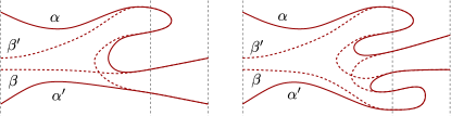
Figure 4: (Color online) Examples of four trajectories $\alpha$, $\beta$, $\alpha^{\prime}$, and $\beta^{\prime}$ contributing to $\langle{\cal T}(n;p^{\prime},p){\cal T}(n;p^{\prime\prime},p^{\prime})\rangle_{n}$ for an array of chaotic cavities, where the average is taken with respect to the Fermi energy of the $n$th cavity only. The examples shown here have a non-diagonal pairing with $m_{\alpha}=m_{\beta^{\prime}}=2$, $m_{\alpha^{\prime}}=m_{\beta}=1$ (left panel) and $m_{\alpha}=m_{\beta^{\prime}}=m_{\alpha^{\prime}}=m_{\beta}=2$ (right panel). In the $n$th cavity, the trajectories $\alpha$ and $\alpha^{\prime}$ are piecewise equal to $\beta$ and $\beta^{\prime}$, up to quantum uncertainties.

The leading non-diagonal pairing appears if one pairs the first $u$ segments of $\alpha$ with the first $u$ segments of $\beta^{\prime}$, and the last $m_{\alpha}-u$ segments of $\alpha$ with the last $m_{\alpha}-u$ segments of $\beta$, as well as the first $v$ segments of $\alpha^{\prime}$ with the first $v$ segments of $\beta$, and the last $m_{\alpha^{\prime}}-v$ segments of $\alpha^{\prime}$ with the last $m_{\alpha^{\prime}}-v$ segments of $\beta^{\prime}$, where $u=1,\ldots,m_{\alpha}-1$ and $v=1,\ldots,m_{\alpha}^{\prime}-1$ are integers. Two examples, with $m_{\alpha}=2$, $m_{\alpha^{\prime}}=1$, $u=1$, and $v=0$, and with $m_{\alpha}=m_{\alpha^{\prime}}=2$ and $u=v=1$, are shown in Fig. 4. One then finds

$$\langle\delta{\cal T}\delta{\cal T}\rangle^{\rm non\,diag}_{n} = \frac{1}{g_{\rm c}}[{\cal F}(p_{1}^{\prime},p_{2}){\cal T}(p_{1},p_{2}^{\prime})$$

$$\mbox{}+{\cal F}(p_{1},p_{2}^{\prime}){\cal T}(p_{1}^{\prime},p_{2})$$

$$\mbox{}+{\cal T}(p_{1},p_{2}^{\prime}){\cal T}(p_{1}^{\prime},p_{2})]+{\cal O}(1/g_{\rm c}^{2}),$$

where ${\cal T}(p_{1},p_{2})={\cal T}(n-1;p_{1},p_{2})$ and ${\cal F}(p_{1},p_{2})={\cal F}(n-1;p_{1},p_{2})$, with

$${\cal F}(n) = \mbox{tr}\,S_{12}S^{\dagger}_{22}S_{22}S^{\dagger}_{12}$$ (29)

$$= {\cal T}(n)-{\cal T}(n)^{2}.$$

Other pairings give contributions of order $1/g_{\rm c}^{2}$ or smaller.

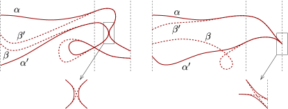
Figure 5: (Color online) Two examples of a set of four trajectories contributing to $\langle{\cal T}{\cal T}^{\prime}\rangle_{n}$ that have a small-angle encounter in the $n$th cavity. For the left panel the encounter is in the interior of the $n$th cavity; For the right panel it touches the exit contact.

The second contribution to the fluctuations of $\delta{\cal T}$ comes from trajectories with a small-angle encounter in the $n$th cavity. Since we only need fluctuations of $\delta{\cal T}$ to leading order in $1/g_{\rm c}$, it is sufficient to consider trajectories with one small-angle encounter only. Taking the small-angle encounter to be between the segments $\alpha_{u}$, $\beta^{\prime}_{u}$, $\alpha^{\prime}_{v}$, and $\beta^{\prime}_{v}$, with $1\leq u,v\leq m,m^{\prime}$, and pairing the first $u-1$ segments of $\alpha$ with the first $u-1$ segments of $\beta^{\prime}$, and the last $m-u$ segments of $\alpha$ with the last $m-u$ segments of $\beta$, as well as the first $v-1$ segments of $\alpha^{\prime}$ with the first $v-1$ segments of $\beta$, and the last $m^{\prime}-v$ segments of $\alpha^{\prime}$ with the last $m^{\prime}-v$ segments of $\beta^{\prime}$, we find

$$\langle\delta{\cal T}\delta{\cal T}\rangle^{\rm enc}_{n} = -{\cal T}(p_{1},p_{2}^{\prime}){\cal T}(p_{1}^{\prime},p_{2})\sum_{u,v=1}^{\infty}\sum_{m=u}^{\infty}\sum_{m^{\prime}=v}^{\infty}\frac{(\mbox{tr}\,{\cal R})^{m+m^{\prime}-2}}{2^{m+m^{\prime}+1}g_{\rm c}^{m+m^{\prime}-1}}$$ (30)

$$\mbox{}+{\cal T}(p_{1},p_{2}^{\prime}){\cal T}(p_{1}^{\prime},p_{2})\sum_{m=1}^{\infty}\sum_{m^{\prime}=1}^{\infty}\frac{(\mbox{tr}\,{\cal R})^{m+m^{\prime}-2}}{2^{m+m^{\prime}}g_{\rm c}^{m+m^{\prime}-1}}$$

$$= -\frac{1}{g_{\rm c}}{\cal T}(p_{1},p_{2}^{\prime}){\cal T}(p_{1}^{\prime},p_{2}).$$

where the first line comes from encounters in the interior of the $n$th cavity and the second line comes from encounters that touch the exit contact.Whitney and Jacquod (2006); Brouwer and Rahav (2006b) Examples of the two terms for $m=m^{\prime}=1$ are shown in Fig. 5. [We do not need to consider encounters that touch the contact between the $(n-1)$st cavity and the $n$th cavity, because the contribution from such encounters is included in the (products) of the kernel ${\cal T}$ of the first $n-1$ cavities.]

Combining everything we have

$$\langle\delta{\cal T}(p_{1},p_{2})\delta{\cal T}(p_{1}^{\prime},p_{2}^{\prime})\rangle_{n} = \frac{1}{g_{\rm c}}[{\cal F}(p_{1}^{\prime},p_{2}){\cal T}(p_{1},p_{2}^{\prime})$$ (31)

$$\mbox{}+{\cal F}(p_{1},p_{2}^{\prime}){\cal T}(p_{1}^{\prime},p_{2})]$$

$$\mbox{}+{\cal O}(1/g_{\rm c}^{2}).$$

Equation (31) is the semiclassical equivalent of Eq. (5).

Higher cumulants of $\delta{\cal T}$ can be calculated in the same way. For the $k$th cumulant, one finds that only pairings that involve trajectories out of all $k$ factors ${\cal T}$ contribute. Each additional factor ${\cal T}$ involved in the pairing scheme contributes an additional factor $1/g_{\rm c}$, which is why all cumulants with $k>2$ are of sub-leading order in $1/g_{\rm c}$.

Together, Eqs. (22) and (31) form the semiclassical equivalent of the stochastic recursion relation (4) used in the fully quantum mechanical theory of localization in disordered quasi-one dimensional wires. In the limit $g_{\rm c}\to\infty$ at fixed $n/g_{\rm c}$, Eqs. (22) and (31) can be mapped to stochastic differential equation for the eigenvalues of ${\cal T}$, which will be formally equivalent to the DMPK equation. The DMPK equation, in turn, provides a full description of localization in quasi-one dimensional wires.Dorokhov (1982); Mello et al. (1988); Beenakker (1997)

IV.2 Presence of time-reversal symmetry

In the presence of time-reversal symmetry both the average $\langle\delta{\cal T}\rangle_{n}$ and the covariance $\langle\delta{\cal T}\delta{\cal T}^{\prime}\rangle_{n}$ are different. In both cases the difference appears because one can pair time-reversed trajectories when taking the ensemble average in the $n$th cavity.

There are two additional contributions to the average $\langle\delta{\cal T}\rangle_{n}$. The first of these arises from the diagonal approximation for the average in the $n$th cavity. As before, we define the number $m=m_{\alpha}=m_{\beta}$ as the number of times the trajectories $\alpha$ and $\beta$ enter the $n$th cavity from the $(n-1)$st cavity. The first additional contribution to $\langle\delta{\cal T}\rangle_{n}$ then involves the pairing of segments $\alpha_{u+j}$ with the time-reversed of $\beta_{u+v-j-1}$, $j=0,\ldots,v-1$, and $1\leq u\leq u+v<m$,

$$\langle\delta{\cal T}\rangle_{n}^{(1)} = {\cal F}\sum_{v=1}^{\infty}\sum_{m=v+1}^{\infty}\frac{1}{2^{m}g_{\rm c}^{m-1}}(\mbox{tr}\,{\cal R})^{m-2}$$ (32)

$$\mbox{}+{\cal T}\sum_{u=1}^{\infty}\sum_{v=1}^{\infty}\sum_{m=u+v+1}^{\infty}\frac{\mbox{tr}\,{\cal R}^{2}}{2^{m}g_{\rm c}^{m-1}}(\mbox{tr}\,{\cal R})^{m-3}$$

$$= \frac{1}{g_{\rm c}}\left({\cal F}+{\cal T}\right).$$

Examples for trajectory pairs contributing to the first and second line in Eq. (32) are shown in Fig. 6. The second contribution comes from small-angle encounters inside $n$th cavity involving the segments $\alpha_{u}$, $\beta_{u}$, $\alpha_{u+v}$, and $\beta_{u+v}$, where $1\leq u\leq u+v\leq m$. For this contribution one finds

$$\langle\delta{\cal T}\rangle_{n}^{(2)} = -\frac{2}{g_{\rm c}}{\cal T}.$$ (33)

Examples of trajectory pairs contributing to $\langle\delta{\cal T}^{(2)}\rangle_{n}$ are shown in Fig. 7. Using ${\cal F}={\cal T}-{\cal T}^{2}$ and adding these two contributions to Eq. (22) one finds

$$\langle\delta{\cal T}\rangle_{n} = -\frac{1}{g_{\rm c}}{\cal T}(n-1)\mbox{tr}\,{\cal T}(n-1)-\frac{1}{g_{\rm c}}{\cal T}^{2},$$ (34)

up to corrections of order $1/g_{\rm c}^{2}$.

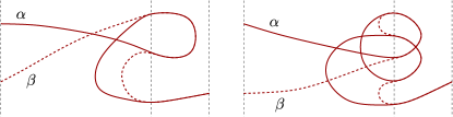
Figure 6: (Color online) Two examples of trajectory pairs contributing to $\langle\delta{\cal T}\rangle_{n}$ in the presence of time-reversal symmetry.

For the fluctuations of $\delta{\cal T}$ in the presence of time-reversal symmetry one finds an extra contribution from pairing $\alpha_{j}$ with the time-reversed of $\beta^{\prime}_{u+1-j}$, $j=1,\ldots,u$, or $\alpha^{\prime}_{j}$ with the time-reversed of $\beta_{u+1-j}$, while following diagonal pairing rules for all other segments. Proceeding as before, we find

$$\langle\delta{\cal T}(p_{1},p_{2})\delta{\cal T}(p_{1}^{\prime},p_{2}^{\prime})\rangle_{n} = \frac{1}{g_{\rm c}}[{\cal F}(p_{1}^{\prime},p_{2}){\cal T}(p_{1},p_{2}^{\prime})$$ (35)

$$\mbox{}+{\cal F}(p_{1},p_{2}^{\prime}){\cal T}(p_{1}^{\prime},p_{2})$$

$$\mbox{}+2{\cal G}(p,p_{1}^{\prime}){\cal G}^{\dagger}(p_{2},p_{2}^{\prime})]$$

$$\mbox{}+{\cal O}(1/g_{\rm c}^{2}).$$

where

$${\cal G}(p,p^{\prime}) = {\cal G}(p^{\prime},p)$$ (36)

$$= [S_{12}S_{22}^{\dagger}S_{21}](p,p^{\prime}).$$

The stochastic process defined by Eqs. (34) and (35) precisely mirrors the stochastic process (4) for the quantum mechanical matrix ${\cal T}^{\rm q}=S_{12}^{\rm q}S_{12}^{{\rm q}\dagger}$.

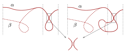
Figure 7: (Color online) Two examples of trajectory pairs contributing to $\langle\delta{\cal T}\rangle_{n}$ in the presence of time-reversal symmetry. The trajectory pairs have a small-angle encounter in the $n$th cavity.

IV.3 Recursion relations for the moments of ${\cal T}$

The direct construction of recursion relations for the moments of ${\cal T}$ is an alternative to the stochastic approach that avoids extending the use of the properties (i) and (ii) of Sec. III to sample-specific quantities and the necessity to define a statistical ensemble by varying the Fermi energy or shape of each cavity individually. The construction of recursion relations for moments of ${\cal T}$ proceeds in the very same manner as the construction of the stochastic recursion relations for ${\cal T}$, with the additional requirement that trajectories are piecewise paired in all $n$ cavities, not only in the $n$th cavity. Since the arguments of the preceding section did not rely on the structure of the trajectories in the first $n-1$ cavities, one immediately concludes that the recursion relations for the moments of ${\cal T}$ derived this way are identical to the recursion relations for the moments of ${\cal T}$ one obtains from the stochastic approach. Starting from the stochastic recursion relations (22) and (31) or (34) and (35) one arrives at the same hierarchy of recursion relations (7) derived for an array of disordered cavities.

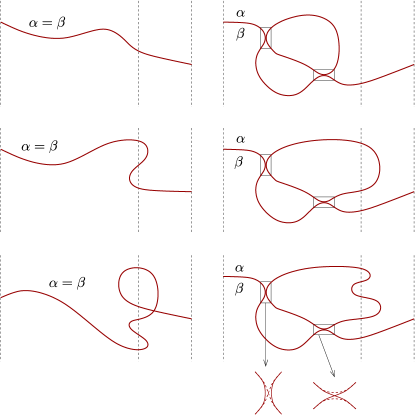
Figure 8: (Color online) Examples of trajectory pairs contributing to the full average $\langle{\cal T}(n)\rangle$ in the absence of time-reversal symmetry. The trajectory pairs have $m=1$ (top), $m=2$ (center), and $m=3$ (bottom). The left panel shows trajectory pairs without small-angle self intersections; The right panel shows trajectory pairs with two small-angle self intersections in the first $n-1$ cavities.

We illustrate this procedure for the recursion relation for the first moment $\langle\mbox{tr}\,{\cal T}(n)\rangle$ in the absence of time-reversal symmetry. Following the rules of the semiclassical formalism, the average $\langle\mbox{tr}\,{\cal T}(n)\rangle$ is determined by trajectory pairs $\alpha$, $\beta$ that are piecewise paired throughout the entire array of cavities. The trajectories can have small-angle self encounters, at which the pairing between $\alpha$ and $\beta$ can be changed. Each pair of trajectories is classified by the number $m$ of times the trajectories enter the $n$th cavity from the $(n-1)$st cavity. The $m$ segments of each trajectory in the $n$th cavity are labeled $\alpha_{1},\ldots,\alpha_{m}$ and $\beta_{1},\ldots,\beta_{m}$.

As in Sec. IV.1, it will be sufficient to consider pairs of trajectories in which each segment $\alpha_{j}$ is paired with the corresponding segment $\beta_{j}$, $j=1,\ldots,m$. Trajectory pairs with self encounters in the $n$th cavity or with non-diagonal pairings in the $n$th cavity give contributions to $\delta\langle\mbox{tr}\,{\cal T}\rangle$ that are a factor $1/g_{\rm c}$ smaller than the leading contribution. For the diagonal pairing, the remaining $m$ segments of the trajectories $\alpha$ and $\beta$ that reside in the first $n-1$ cavities precisely generate $\langle\mbox{tr}\,{\cal T}(n-1)[\mbox{tr}\,{\cal R}(n-1)]^{m-1}\rangle$, where the averaging brackets refer to variations of the Fermi energy for the entire array of cavities. Hence, we find

$$\langle\mbox{tr}\,{\cal T}(n)\rangle = \sum_{m=1}^{\infty}\frac{\left\langle\mbox{tr}\,{\cal T}(n-1)[\mbox{tr}\,{\cal R}(n-1)]^{m-1}\right\rangle}{2^{m}g_{\rm c}^{m-1}}$$ (37)

$$= \left\langle\frac{g_{\rm c}\mbox{tr}\,{\cal T}(n-1)}{2g_{\rm c}-\mbox{tr}\,{\cal R}(n-1)}\right\rangle.$$

A schematic representation of trajectory pairs contributing to Eq. (37) with up to two self-encounters in the first $n-1$ cavities are shown in Fig. 8. Using unitarity to express ${\cal R}$ in terms of ${\cal T}$ and subtracting $\langle\mbox{tr}\,{\cal T}(n-1)\rangle$, one then finds

$$\delta\langle\mbox{tr}\,{\cal T}(n)\rangle = \langle\mbox{tr}\,{\cal T}(n)\rangle-\langle\mbox{tr}\,{\cal T}(n-1)\rangle$$ (38)

$$= \frac{1}{g_{\rm c}}\langle(\mbox{tr}\,{\cal T}(n-1))^{2}\rangle.$$

This is the same equation as one obtains from taking the average of the increment $\mbox{tr}\,\delta{\cal T}$ in the stochastic approach.

V Field theory formulation

In this section, we will approach the localization phenomenon from a different perspective. We will use that the quantum dot array depicted in Fig. 1 supports hierarchies of different types of field-fluctuations in a field-theoretic description. These fluctuations reflect the fate of density distributions in classical phase space under the dynamical evolution of the system. Each of these fluctuations, thus, comes with a characteristic ‘relaxation time’, i.e., a time scale on which the fluctuation decays. (For example, fluctuations inhomogeneous in the sector of phase space describing an individual quantum dot will decay on a time scale comparable to the time of flight through the dot, etc.) In the description of low energy phenomena such as the zero frequency (DC) conductance, modes operating at short time scales can be treated perturbatively. Their feedback into the sector of long time scales then stabilizes a ‘low energy theory’. In the following, we will derive a theory that is minimal in that it contains information equivalent to that stored in the Fokker-Planck equation of localization. The strategy pursued here parallels one applied previously Altland and Zirnbauer (1996a) to the problem of dynamical localization in the quantum kicked rotor (also known as the “standard map”.) One difference is that the spectrum of different modes encountered in the present problem happens to be more complex. Our logics also resembles that of Ref. Müller et al., 2007b, where it had been shown that the relevant low energy theory of an ergodic quantum system contains the information otherwise stored in random matrix theory.

Technically, our discussion will be based on a formulation of the array in terms of the ballistic nonlinear $\sigma$-model.Muzykantskiǐ and Khmelnitskiǐ (1995); Andreev et al. (1996) A quadratic approximation in energetically high lying modes generates an effective low energy theory wherein each quantum dot is treated as a structureless (‘ergodic’) entity. This theory will be equivalent to the celebrated nonlinear $\sigma$-model of disordered quantum wires,Efetov (1997) a model that predicts Anderson localization on large length scales. We will see that the parameters stabilizing the hierarchical mode integration are the same as those utilized in previous sections of this paper.

Conceptually, the hierarchical scheme is an alternative to an indiscriminate perturbative integration over all modes in one go. That latter scheme would be essentially equivalent (see Ref. Müller et al. (2007b) for a discussion in the context of spectral statistics.) to a semiclassical expansion in terms of paired trajectories. In this sense, the hierarchical mode integration processes the information stored in the statistics of trajectories by different means.

V.1 Field theory of the quantum dot array

Our starting point will be the description of the quantum dot array in terms of the supersymmetric ballistic nonlinear $\sigma$-model. This theory is obtained by averaging exact functional representations of Green functions over an energy interval of width $\Delta E$ centered around the uniform Fermi energy $E_{F}$ of the array. A subsequent saddle point approximation (stabilized in the parameter $E_{F}/\Delta E\gg 1$) then obtains a field theory in classical phase defined by

$$Z \equiv \int DT\,\exp(-S[T]),$$ (39)

with

$$S[T] = \frac{\beta\pi\hbar\nu}{2}\int_{\Gamma}(d{\bf x})\,{\rm tr}\Big{(}T\ast\Lambda\{H,T^{-1}\}\Big{)}$$ (40)

$$\mbox{}+S_{\rm reg}[T].$$

The integration variables in (39), $T({\bf x})=\{T^{\alpha\alpha^{\prime}}({\bf x})\}$ are (super) matrix valued fields defined on shells $\Gamma=\{{\bf x}|H({\bf x})=E_{0}\}$ of constant energy in classical phase space. Further, ${\bf x}\equiv({\bf q},{\bf p})$ where ${\bf q}$ and ${\bf p}$ are coordinates and momenta, respectively, $H({\bf x})$ is the Hamiltonian function of the system, the integral over the energy-shell is normalized to the (spatial) volume of the system, $\int_{\Gamma}(d{\bf x})={\rm Vol}$, and $\nu$ is the single particle density of states per volume, $\nu=1/(\Delta{\rm\,Vol})$. For time reversal and spin rotation invariant systems (orthogonal symmetry class, $\beta=1$), the ‘internal’ structure of the matrices $T^{\alpha\alpha^{\prime}}$ is described by a composite index $\alpha=(a,r,t)$, where $a=+/-$ discriminates between the advanced and retarded sector of the theory, $r={\rm b},{\rm f}$ discriminates between commuting and anticommuting sectors, and $t=1,2$ accounts for the operation of time reversal. Time reversal symmetry reflects in the relation $(\tau T^{T}\tau^{-1})({\bf q},-{\bf p})=T^{-1}({\bf q},{\bf p})$, where $\tau$ is a fixed matrix whose detailed structure will not be of concern throughout. For time reversal non-invariant systems (unitary symmetry, $\beta=2$) no time-reversal structure exists and $\alpha=(a,r)$. In either case, the matrices $T$ carry a coset space structure in the sense that configurations $T$ and $TK$ are to be identified if $[K,\Lambda]=0$, where $\Lambda=\sigma_{3}^{\rm ar}$ and “ar” stands for action in advanced/retarded space. Finally, the regulatory action

$$S_{\rm reg}[T]\equiv\delta\int_{\Gamma}(d{\bf x})\,{\rm str}\Big{(}\Lambda T^{-1}\ast\Lambda T\Big{)},\ \ \delta\downarrow 0$$

determines the ‘causality’ of field fluctuations, but will otherwise not be of much relevance throughout.

The fluctuation behavior of the fields $T$ in (39) is governed by the classical Liouville operator $\{H,\;\}$ (where $\{\;,\;\}$ is the Poisson bracket.) Quantum mechanics enters the problem through the presence of Moyal products “$\ast$” in (39). In essence, this product operationfoot5 limits the maximum resolution of the theory in phase space to scales of the order of a Planck cell. In the following sections we reduce the above ‘bare’ theory to an effective low energy theory describing localization phenomena.

V.2 Hierarchical mode integration

Before turning to the technicalities of the mode integration, let us describe the relevant hierarchies in qualitative terms: fluctuations inhomogeneous in the phase space sector representing individual dots are expected to relax on short time scales comparable to the time of flight across the dot, $t_{f}$.foot6 On the other hand, relative fluctuations in the configuration of different dots can survive up to time scales of the order of the dwell time $\tau_{\rm D}\gg t_{f}$. To describe this hierarchical decay profile within our field theory framework, we focus on a section of the array containing two neighboring quantum dots (cf. Fig. 9). The fields $T({\bf x})$ representing phase space fluctuations in this subsystem may be decomposed as $T=T_{s}T_{f}$, where $T_{s,f}$ are ‘slow’ and ‘fast’ fluctuations, respectively. The slow fluctuations are (i) homogeneous within each dot separately. In particular, (ii) they do not vary in any spatial cross section transverse to the array, and (iii) do not depend on momentum. However, (iv) the weakness of the inter-dot coupling ($\tau_{\rm D}\gg t_{f}$) leaves room for gradual fluctuations of the slow modes as we pass from one dot into the other. This suggests a parameterization $T_{s}({\bf x})=T_{s}(q)$, where $q$ is the component of ${\bf q}$ parallel to the longitudinal direction of the two-dot system. Point (i) above means that $T_{s}(q\ll 0)=T_{L}$ and $T_{s}(q\gg 0)=T_{R}$, where $T_{L,R}$ are the constant slow mode configurations of the left and the right dot, respectively. As we are going to check in a self consistent manner, (v) relative fluctuations between left and right dot are suppressed (in a parameter of the order of the number of transverse quantum channels supported by the connector region) so that a leading order expansion in relative fluctuations $T^{\vphantom{-1}}_{L}T_{R}^{-1}$ is sufficient. (Conceptually, this expansion is equivalent to the Kramers-Moyal expansion employed in the derivation of the Fokker-Planck equation above.)

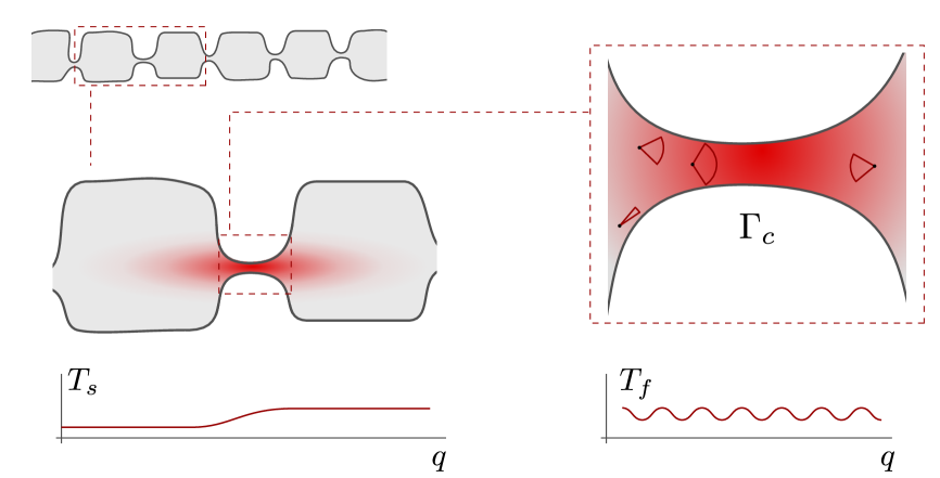
Figure 9: (Color online) Top left: cartoon of an array of weakly coupled quantum dots. Center left: cut region containing two dots. The shaded region indicates the real space support of the coupling phase space $\Gamma_{c}$. Bottom left: plot indicating the profile of weakly fluctuating field configurations: constancy throughout each dot, gradual variation in the coupling region. Center right: zoom into the coupling region. The phase space region $\Gamma_{c}$ contains points ${\bf x}=({\bf q},{\bf n})$ that will migrate between the two dots in short time, i.e., without undergoing back scattering. (The opening angles represent those directions ${\bf n}$ that meet this criterion.) Bottom right: schematic plot of real space profile of phase space fluctuations generating the inter-dot coupling.

The field $T_{f}$ encapsulates all other fluctuations, i.e., fluctuations that do not meet the criteria (i-v). Generic fluctuations of this type – think of fast fluctuations deep inside the phase space of one of the dots – are strongly gapped and do not couple to the slow fluctuations. (Formally, this decoupling manifests itself in an effective ‘orthogonality’ between the modes representing these fluctuations.) However, there is one sector of phase space, $\Gamma_{c}$, in which fast and slow fluctuations talk to each other. The domain $\Gamma_{c}$ includes all points in phase space which pass from one dot to the other in a time of order $t_{f}\ll\tau_{\rm D}$, much smaller than the typical dwell time (cf. the shaded area in Fig. 9). This region is special in that it overlaps with the domain of gradual variation of the slow fields (cf. point (iv) above.) As we will see, a perturbative integration over fast fields in $\Gamma_{c}$ effectively determines the slow field coupling between the two dots.

To prepare the integration over the fast fields in $\Gamma_{c}$, we need to bring the notation to a more explicit level: assuming that the bulk dynamics is ballistic, $\{H,\;\}=v_{F}{\bf n}\cdot\nabla$ where ${\bf n}$ is the unit vector in momentum space, and $v_{F}$ the Fermi velocity. Current conservation in the specular reflection at the system boundaries translates to the effective boundary condition $f({\bf x},{\bf n})=f({\bf x},\bar{\bf n})$, where $f$ is a phase function subject to the action of $\{H,\;\}$, ${\bf x}$ a boundary point and $\bar{\bf n}$ the direction vector with flipped normal component.

We next parameterize fluctuations as $T_{s,f}=\exp(W_{s,f})$, where the field generators carry a block structure (in advanced/retarded space),

$$W_{s,f}=\left(\begin{smallmatrix}&B_{s,f}\\ \bar{B}_{s,f}&\end{smallmatrix}\right).$$

(For further technical details on this representation we refer to Ref. Efetov, 1997.) We now substitute these generators into the action, expand to leading order in $W_{f}$, and integrate. This leads to the effective action

$$S_{\rm eff}[T_{s}]=\frac{1}{2}\left\langle\left(S^{(1)}[T_{s},W_{f}]\right)^{2}\right\rangle+S_{\rm reg}[T_{s}],$$ (41)

where $\langle\dots\rangle\equiv\int DW_{f}\,\exp(-S^{(2)}[\openone,W_{f}])(\dots)$, and $S^{(n)}[T_{s},W_{f}]$ is of $n$th order in $W_{f}$. Due to the isotropy of $T_{s}$ in momentum space and the linearity of the Poisson bracket in ${\bf n}$, the action does not contain a contribution of zeroth oder in the fast fields. The dominant contribution to the coupling between fast and slow fluctuations is given by the linear term,

$$S^{(1)}[T_{s},W_{f}] =\beta\pi\hbar\nu v_{F}\int_{\Gamma_{c}}d{\bf q}d{\bf n}\,n_{\parallel}\,{\rm str}\left[W_{s}({\bf q},{\bf n})\Phi(q)\right]$$ (42)

where we have introduced the abbreviation $\Phi\equiv(\partial_{q}T_{s})\ast\Lambda T_{s}^{-1}$, the integration over the direction of momentum is normalized as $\int d{\bf n}=1$, $n_{\parallel}$ is the component of ${\bf n}$ parallel to the longitudinal direction and the Moyal product has been omitted (which is permissible due to the general relation $\int(d{\bf x})(f\ast g)({\bf x})=\int(d{\bf x})(f\,g)({\bf x})$ for the integrated product of two functions – presently, matrix elements of $\Phi$ and $W$ – in phase space.)

Neglecting contributions of $\mathcal{O}(\Phi W_{f}^{2})$ (as compared to the $\mathcal{O}(\Phi W_{f})$-terms above) the quadratic $W_{s}$-action is given by

$$S^{(2)}[T_{s},W_{f}] \simeq S^{(2)}[\openone,W_{f}]$$

$$= \beta\pi\hbar\nu\int_{\Gamma_{c}}d{\bf q}d{\bf n}\,{\rm str}(\bar{B}_{f}({\bf q},{\bf n})(v_{F}{\bf n}\cdot\nabla+\delta)B_{f}({\bf q},{\bf n})).$$

Fast field fluctuations can now be integrated out according to the prescription $\langle{\rm str}(A({\bf q},{\bf n})B_{f}({\bf q},{\bf n}))\;{\rm str}(\bar{A}({\bf q}^{\prime},{\bf n}^{\prime})\bar{B}_{f}({\bf q}^{\prime},{\bf n}^{\prime}))\rangle=\delta({\bf n}-{\bf n}^{\prime})\Pi({\bf q},{\bf q}^{\prime};{\bf n})$, where

$$\Pi({\bf q},{\bf q}^{\prime};{\bf n})\equiv\frac{1}{\beta\pi\hbar\nu}(v_{F}{\bf n}\cdot\nabla+\delta)^{-1}({\bf q},{\bf q}^{\prime}).$$

Specifically, the effective action is given by

$$S_{\rm eff}[T_{s}] = (\beta\pi\hbar\nu v_{F})^{2}\int_{\Gamma_{c}}d{\bf q}d{\bf q}^{\prime}d{\bf n}\,n_{\parallel}^{2}\mbox{str}\,\left(\Phi_{21}(q)\Phi_{12}(q)\right)\Pi({\bf q},{\bf q}^{\prime};{\bf n})$$

So far, we have not made reference to the specific properties of the phase space region $\Gamma_{c}$. We now assume that the corridor connecting the dots has wave-guide properties, in that it (a) does not contain significant backscattering, and (b) the restriction of the Liouville operator to $\Gamma_{c}$ has plane-wave like eigenfunctions characterized by a conserved longitudinal/transverse momentum ${\bf k}_{\perp}/k$. We also assume that (c) the slow fields smoothly interpolate between $T_{L}$ and $T_{R}$ in a region centered around the longitudinal coordinate $q=0$. The presumed proximity $T_{L}\simeq T_{R}$ implies that $\Phi(q)\simeq\partial_{q}W(q)\Lambda$ can be linearized, where we suppressed the slow field index ‘$s$’ for notational transparency. Under these circumstances, and noting that the integration over ${\bf q}_{\perp}$ implies a projection onto the zero-momentum sector ${\bf k}_{\perp}=0$, we obtain

$$S_{\rm eff}[T_{s}] =-\beta\pi\hbar\nu S_{c}v^{2}_{F}\int_{-c}^{c}dqdq^{\prime}{\rm\,str}\left(\Phi_{21}(q)\Phi_{12}(q^{\prime})\right)\int d{\bf n}\,n^{2}_{\parallel}\int\frac{dk}{2\pi}\frac{e^{ik(q-q^{\prime})}}{iv_{F}n_{\parallel}k+\delta}=$$

$$=-\beta\pi\hbar\nu S_{c}v_{F}\int_{-c}^{c}dqdq^{\prime}{\rm\,str}\left(\Phi_{21}(q)\Phi_{12}(q^{\prime})\right)\underbrace{\int d{\bf n}\,|n_{\parallel}|\Theta\left(\frac{q-q^{\prime}}{n_{\parallel}}\right)}_{={\rm const.}}=$$

$$={\rm const.}\times\hbar\nu S_{c}v_{F}\,{\rm str}((\bar{B}_{R}-\bar{B}_{L})(B_{R}-B_{L})),$$

where the indices refer to “ar”-space, ${\rm const.}=\mathcal{O}(1)$ is a constant, $S_{c}$ the transverse cross section of the contact, and $B_{R,L}$ are the generators of the slow fields in the left and the right dot, respectively. Noting that the density of states per volume, $\nu\sim mk_{F}^{d-2}$ (where $k_{F}=v_{F}m$ is the Fermi momentum) and $S_{c}k_{f}^{d-1}\sim N$ is proportional to the number of transverse channels, $N$, supported by the connector region, the prefactor can be written as ${\rm const.}\times N\gg 1$, a number which we assume large lest a semiclassical description of the contact becomes meaningless. We also note that the quadratic form may be replaced by its unique rotationally invariant generalization to the full field manifold, ${\rm str}((\bar{B}_{R}-\bar{B}_{L})(B_{R}-B_{L}))\to\frac{1}{4}{\rm str}(Q_{L}Q_{R})$, where $Q=T\Lambda T^{-1}$. While a quadratic expansion of the latter expression reproduces the bilinear term, the largeness of $N$ implies that typical values contributing to the $B$-integration, $B\sim N^{-1/2}\ll 1$, which means that non-linear contributions become inessential in the limit of large channel numbers. We thus conclude that the coupling term can be rewritten as

$$S_{\rm eff}[Q]={\rm const.}\times N{\,\rm str}(Q_{L}Q_{R}).$$

Finally, the obvious generalization of the above two-dot construction to an entire quantum dot array reads as

$$S_{\rm eff}[Q]={\rm const.}\times\frac{1}{\tau_{\rm D}\Delta}\sum_{m}{\rm str}(Q_{m}Q_{m+1}),$$ (43)

where $Q_{m}$ is the $Q$-matrix representing the $m$-th dot and we used that the channel number $N\sim(\tau_{\rm D}\Delta)^{-1}$. Before turning to the discussion of localization properties, a few remarks on the construction above are in order.

• Conceptually, the above reduction programs involves three steps: 1) identification of ‘low energy modes’, i.e., modes that decay on the largest time scales of the problem, 2) identification of ‘high energy’, or quickly decaying modes, and 3) perturbative integration over those fast modes that will conceivably couple to the slow modes. In principle, that integration can be explicated for any fluctuation in the problem. In practice, however, only few modes will effectively couple to the slow degrees of freedom, and these relevant fluctuations are best identified by semiclassical considerations:

• Semiclassically speaking, a ‘mode’ represents the coherent propagation of a retarded and an advanced Feynman amplitude along classical trajectories in phase space. Locally, the semiclassical dynamics of such composites is described by the Liouville operator, as is manifest in the action (39). This trajectory interpretation helps in identifying the relevant fast modes. E.g., in the system depicted in Fig. 9, the coupling between the ergodic slow modes of each dot, $Q_{m}$, is dominated by trajectories swiftly propagating from one dot to the other, i.e., modes emanating at phase space points ${\bf x}\in\Gamma_{c}$.

• Although this identification of fast modes rests on specific model assumptions (no backscattering in the contact region, etc.), the result (43) is reasonably universal. For example, a somewhat more elaborate construction will show that the same action describes connector regions containing chaotic scattering and momentum relaxation by themselves. (The latter complication would manifest itself in an altered value of $\tau_{\rm D}$, though.) Generally speaking, the low energy physics of the system will reduce to $S_{\rm eff}$, as long as the dots are isolated from each other in the sense $t_{f}\ll\tau_{\rm D}$.

V.3 Localization from the effective action (43)

The effective action (43) is equivalent to a ‘lattice version’ of the diffusive nonlinear $\sigma$-model of quasi-one dimensional disordered wires. Indeed, we may pass to a continuum limit

$$\frac{1}{\tau_{\rm D}\Delta}\sum_{m}{\rm str}(Q_{m}Q_{m+1})\to\frac{a}{\tau_{\rm D}\Delta}\int_{0}^{L}dx\,{\rm str}(\partial Q\partial Q),$$

where $Q_{m}\to Q(x)$ is replaced by a smooth field, $x=ma$, and $a$ the spacing between the dots. Comparing to the standard form of the diffusive model,Efetov (1997) where the action is $\sim\xi\int dx\,{\rm str}(\partial Q\partial Q)$ with $\xi$ the localization length, we are led to the identification $\frac{a}{\tau_{\rm D}\Delta}\sim\xi$.

VI Conclusion

In the preceding sections we showed how a theory of Anderson localization can be constructed for a sample in which the microscopic electron dynamics is ballistic, rather than disordered-diffractive. Our theory of “ballistic Anderson localization” paraphrases the scaling approach to localization in disordered quantum wires of Dorokhov, Mello, Pereyra, and Kumar,Dorokhov (1982); Mello et al. (1988) using the language of the trajectory-based semiclassical formalism. As noted in the introduction, the interest of constructing such a semiclassical theory is not the structure of the theory itself or the phenomena it explains. Like most semiclassical theories of quantum corrections in the perturbative regime, the structure of the theory closely resembles the structure of its fully quantum mechanical counterpart for disordered metals, whereas the observed phenomena are the same in the ballistic and disordered cases. Instead, the interest of the semiclassical theory is that it shows how quantum effects that were known from disordered metals arise if the electron dynamics is ballistic.

On hindsight it should not come as a surprise that a theory of ballistic Anderson localization can be constructed by adapting the derivation of the Dorokhov-Mello-Pereyra-Kumar equation for a disordered quantum wire. This point is best made by reconsidering Dorokhov’s original derivation.Dorokhov (1982) In this derivation, impurity scattering is treated in the Born approximation. All quantum mechanical amplitudes are squared into quantum probabilities. Hence, it is sufficient if one can replace the quantum mechanical probabilities by classical ones. Such a replacement is a standard procedure when connecting quantum mechanical and semiclassical theories. Its implementation for the array of chaotic cavities is what is done here.

It is interesting to observe that, while small-angle encounters form a crucial link in our understanding of quantum interference corrections in ballistic conductors, their role is very limited in our description of localization in quasi-one dimension: They serve to cancel spurious contributions from trajectories that enter the last cavity of the array more than twice. (In Dorokhov’s original approach such processes are excluded automatically because of the condition that the length of the wire is increased by an amount $\delta L$ much smaller than the mean free path $l$.Dorokhov (1982); Mello et al. (1988)) Implicitly, small-angle encounters do play a much more important role in our theory, however, because they help to preserve unitarity in the semiclassical theory. Unitarity is a key ingredient of both the quantum-mechanical derivation of the DMPK equation and the present semiclassical derivation. We note that unitarity has played an important role in other extensions of the semiclassical framework beyond its previously assumed domain of validity: it is used to relate weak localization and enhanced backscattering, thus enabling a semiclassical description of weak localization without reference to small-angle encounters,Baranger et al. (1993a, b); Argaman (1995) and it is used to obtain an alternative expression for the spectral form factor, allowing its calculation in the non-perturbative regime by considering periodic orbits of duration below the Heisenberg time only.Keating and Müller (2007)

We have also shown that the dynamical information entering the semiclassical approach can be processed by different means to derive an effective low energy field theory of the system. This latter approach is based on the concept of ‘modes’, fluctuations in phase space decaying on parametrically different time scales. A successive integration over short lived modes stabilizes an effective action of the most persistent modes in the fluctuation spectrum. In the present context, that low energy limit turned out to be equivalent to the diffusive nonlinear $\sigma$-model of disordered wires. While the field theory approach is arguably less explicit than the direct classification of trajectories, it enjoys the advantage of high computational efficiency, a paradigm previously exemplified on the problem of universal spectral correlations.Müller et al. (2007b) For example, the above mentioned condition of unitarity, as well as the symmetries relating trajectories to their time reversed are built into the field theory approach from the outset; there is no need for explicit bookkeeping in terms of encounter processes. The price to be payed for this compactness in the description is a higher level of abstraction, though.

References

- Akkermans et al. (1995) E. Akkermans, G. Montambaux, J.-L. Pichard, and J. Zinn-Justin, eds., Mesoscopic Quantum Physics (North-Holland, 1995).
- Imry (2002) Y. Imry, Introduction to mesoscopic physics (Oxford University Press, 2002).
- Anderson (1958) P. W. Anderson, Phys. Rev. 109, 1492 (1958).
- Abrahams et al. (1979) E. Abrahams, P. W. Anderson, D. C. Licciardello, and T. V. Ramakrishnan, Phys. Rev. Lett. 42, 673 (1979).
- Stone (1995) A. D. Stone, in Mesoscopic Quantum Physics, edited by E. Akkermans, G. Montambaux, J.-L. Pichard, and J. Zinn-Justin (North-Holland, 1995).
- Nakamura and Harayama (2004) K. Nakamura and T. Harayama, Quantum Chaos and Quantum Dots (Oxford University Press, 2004).
- (7) This expectation holds only if the relevant electronic time scales exceed the “Ehrenfest time”, the minimum time after which quantum effects appear in ballistic conductors, see Ref. Aleiner and Larkin, 1996.
- Aleiner and Larkin (1996) I. L. Aleiner and A. I. Larkin, Phys. Rev. B 54, 14423 (1996).
- Haake (1991) F. Haake, Quantum Signatures of Chaos (Springer, 1991).
- Kouwenhoven et al. (1997) L. P. Kouwenhoven, C. M. Marcus, P. L. McEuen, S. Tarucha, R. M. Westervelt, and N. S. Wingreen, in Mesoscopic Electron Transport, edited by L. L. Sohn, L. P. Kouwenhoven, and G. Schön (Kluwer, Dordrecht, 1997), vol. 345 of NATO ASI Series E.
- Roukes and Scherer (1989) M. L. Roukes and A. Scherer, Bull. Am. Phys. Soc 34, 633 (1989).
- Ensslin and Petroff (1990) K. Ensslin and P. M. Petroff, Phys. Rev. B 41, 12307 (1990).
- Gutzwiller (1990) M. Gutzwiller, Chaos in Classical and Quantum Mechanics (Springer, New York, 1990).
- Jalabert et al. (1990) R. A. Jalabert, H. U. Baranger, and A. D. Stone, Phys. Rev. Lett. 65, 2442 (1990).
- Sieber and Richter (2001) M. Sieber and K. Richter, Phys. Scripta T90, 128 (2001).
- Sieber (2002) M. Sieber, J. Phys. A: Math. Gen. 35, L613 (2002).
- Richter and Sieber (2002) K. Richter and M. Sieber, Phys. Rev. Lett. 89, 206801 (2002).
- Müller et al. (2007a) S. Müller, S. Heusler, P. Braun, and F. Haake, New. J. Phys. 9, 12 (2007a).
- (19) The relation between quantum corrections and small-angle encounters of classical trajectories was first discovered by Aleiner and Larkin in a formalism which allowed the classical dynamics to be modified by quantum effects, instead of expressing quantum phenomena in terms of classical trajectories only, see Refs. Aleiner and Larkin, 1996, 1997.
- Aleiner and Larkin (1997) I. L. Aleiner and A. I. Larkin, Phys. Rev. E 55, R1243 (1997).
- Müller et al. (2004) S. Müller, S. Heusler, P. Braun, F. Haake, and A. Altland, Phys. Rev. Lett. 93, 014103 (2004).
- Müller et al. (2005) S. Müller, S. Heusler, P. Braun, F. Haake, and A. Altland, Phys. Rev. E 72, 046207 (2005).
- Heusler et al. (2006a) S. Heusler, S. Müller, P. Braun, and F. Haake, Phys. Rev. Lett. 96, 066804 (2006a).
- Whitney and Jacquod (2006) R. S. Whitney and P. Jacquod, Phys. Rev. Lett. 96, 206804 (2006).
- Brouwer and Rahav (2006a) P. W. Brouwer and S. Rahav, Phys. Rev. B 74, 075322 (2006a).
- Berry (1985) M. V. Berry, Proc. R. Soc. London A 400, 229 (1985).
- Heusler et al. (2006b) S. Heusler, S. Müller, A. Altland, P. Braun, and F. Haake, Phys. Rev. Lett. 98, 044103 (2007b).
- Dorokhov (1982) O. N. Dorokhov, Pis’ma Zh. Eksp. Teor. Fiz. 36, 259 (1982) [JETP Lett. 36, 318 (1982)].
- Mello et al. (1988) P. A. Mello, P. Pereyra, and N. Kumar, Ann. Phys. (NY) 181, 290 (1988).
- Efetov and Larkin (1983) K. B. Efetov and A. I. Larkin, Zh. Eksp. Teor. Fiz. 85, 764 (1983) [Sov. Phys. JETP 58, 444 (1983)].
- Efetov (1983) K. B. Efetov, Adv. Phys. 32, 53 (1983).
- (32) This expectation has been verified using numerical simulations in the context of ‘Dynamic localization’,Fishman et al. (1982) Anderson localization in momentum space rather than in real space, which is relevant for certain dynamic systems with a periodic time-dependent Hamiltonian, see Refs. Casati et al., 1979; Shepelyansky, 1986.
- Fishman et al. (1982) S. Fishman, D. R. Grempel, and R. E. Prange, Phys. Rev. Lett. 49, 509 (1982).
- Casati et al. (1979) G. Casati, B. V. Chirikov, J. Ford, and F. M. Izrailev, Lect. Notes Phys. 93, 334 (1979).
- Shepelyansky (1986) D. L. Shepelyansky, Phys. Rev. Lett. 56, 677 (1986).
- Altland and Zirnbauer (1996a) A. Altland and M. R. Zirnbauer, Phys. Rev. Lett. 77, 4536 (1996a).
- Baranger et al. (1993a) H. U. Baranger, R. A. Jalabert, and A. D. Stone, Phys. Rev. Lett. 70, 3876 (1993a).
- Baranger et al. (1993b) H. U. Baranger, R. A. Jalabert, and A. D. Stone, Chaos 3, 665 (1993b).
- Mirlin et al. (1994) A. D. Mirlin, A. Müller-Groeling, and M. R. Zirnbauer, Ann. Phys. (NY) 236, 325 (1994).
- Brouwer and Frahm (1996) P. W. Brouwer and K. Frahm, Phys. Rev. B 53, 1490 (1996).
- Beenakker (1997) C. W. J. Beenakker, Rev. Mod. Phys. 69, 731 (1997).
- Zirnbauer (1992) M. R. Zirnbauer, Phys. Rev. Lett. 69, 1584 (1992).
- (43) This need not be immediately obvious if time-reversal symmetry is present (), since Eq. (5) contains the matrix , which can not be expressed in terms of . Still, the stochastic process defined by Eqs. (4) fully describes the evolution of the eigenvalues of , which can be verified by considering the mean change of or of a product of such traces, which contains in the combination only, .
- Tartakovski (1995) A. V. Tartakovski, Phys. Rev. B 52, 2704 (1995).
- Brouwer (1998) P. W. Brouwer, Phys. Rev. B 57, 10526 (1998).
- Rejaei (1996) B. Rejaei, Phys. Rev. B 53, R13235 (1996).
- Spehner (2003) D. Spehner, J. Phys. A 36, 7269 (2003).
- Turek and Richter (2003) M. Turek and K. Richter, J. Phys. A 36, L455 (2003).
- Rahav and Brouwer (2006) S. Rahav and P. W. Brouwer, Phys. Rev. B 73, 035324 (2006).
- Brouwer (2007) P. W. Brouwer, Phys. Rev. B 76, 165313 (2007).
- Brouwer and Rahav (2006b) P. W. Brouwer and S. Rahav, Phys. Rev. B 74, 085313 (2006b).
- Müller et al. (2007b) J. Müller, T. Micklitz, and A. Altland, Phys. Rev. E 56, 56204 (2007b).
- Muzykantskiǐ and Khmelnitskiǐ (1995) B. A. Muzykantskiǐ and D. E. Khmelnitskiǐ, JETP Lett. 62, 76 (1995).
- Andreev et al. (1996) A. V. Andreev, B. D. Simons, O. Agam, and B. L. Altshuler, Nucl. Phys. B 482, 536 (1996).
- Efetov (1997) K. B. Efetov, Supersymmetry in disorder and chaos (Cambridge University Press, 1997).
- (56) The Moyal product between two phase space functions and is defined as , where is the symplectic unit matrix.
- (57) In fact, the phase space of individual dots supports a small set of fluctuations that decay on time scales longer than the generic : the probability to propagate from a phase space point to the time reversed of a closeby point relaxes on scales , where is the dominant Lyapunov exponent of the system and and are the locally most stable and unstable coordinate of the point in a coordinate system that has as its center. Since the phase space resolution of the quantum theory is limited by , these long time memory effects decay on time scales of the order of the Ehrenfest time . Thus, the decoupled dots have relaxed into a fully ergodic configuration on time scales .
- Argaman (1995) N. Argaman, Phys. Rev. Lett. 75, 2750 (1995).
- Keating and Müller (2007) J. P. Keating and S. Müller, arXiv:0708.2375 (2007).