Dynamic structure factor of Luttinger liquids with quadratic energy dispersion and long-range interactions

Abstract

We calculate the dynamic structure factor $S(\omega,q)$ of spinless fermions in one dimension with quadratic energy dispersion $k^{2}/2m$ and long range density-density interaction whose Fourier transform $f_{q}$ is dominated by small momentum-transfers $q\lesssim q_{0}\ll k_{F}$. Here $q_{0}$ is a momentum-transfer cutoff and $k_{F}$ is the Fermi momentum. Using functional bosonization and the known properties of symmetrized closed fermion loops, we obtain an expansion of the inverse irreducible polarization to second order in the small parameter $q_{0}/k_{F}$. In contrast to perturbation theory based on conventional bosonization, our functional bosonization approach is not plagued by mass-shell singularities. For interactions which can be expanded as $f_{q}=f_{0}+f_{0}^{\prime\prime}q^{2}/2+O(q^{4})$ with $f_{0}^{\prime\prime}\neq 0$ we show that the momentum scale $q_{c}=1/|mf_{0}^{\prime\prime}|$ separates two regimes characterized by a different $q$-dependence of the width $\gamma_{q}$ of the collective zero sound mode and other features of $S(\omega,q)$. For $q_{c}\ll q\ll k_{F}$ all integrations in our functional bosonization result for $S(\omega,q)$ can be evaluated analytically; we find that the line-shape in this regime is non-Lorentzian with an overall width $\gamma_{q}\propto q^{3}/(mq_{c})$ and a threshold singularity $[(\omega-\omega_{q}^{-})\ln^{2}(\omega-\omega_{q}^{-})]^{-1}$ at the lower edge $\omega\rightarrow\omega_{q}^{-}=vq-\gamma_{q}$, where $v$ is the velocity of the zero sound mode. Assuming that higher orders in perturbation theory transform the logarithmic singularity into an algebraic one, we find for the corresponding threshold exponent $\mu_{q}=1-2\eta_{q}$ with $\eta_{q}\propto q_{c}^{2}/q^{2}$. Although for $q\lesssim q_{c}$ we have not succeeded to explicitly evaluate our functional bosonization result for $S(\omega,q)$, we argue that for any one-dimensional model belonging to the Luttinger liquid universality class the width of the zero sound mode scales as $q^{2}/m$ for $q\rightarrow 0$.

I Introduction

Recently several authors have calculated the dynamic structure factor $S(\omega,q)$ in the Luttinger liquid phase of model systems for interacting fermions with non-linear energy dispersion in one spatial dimension Samokhin98 ; Capurro03 ; Pustilnik03 ; Pustilnik06 ; Pustilnik06b ; Cheianov07 ; Teber06 ; Teber07 ; Pereira06 ; Pereira07 ; Pereira07b ; Pirooznia07 ; Schoenhammer07 ; Aristov07 ; Ploetz07 . Mathematically, $S(\omega,q)$ is defined as the spectral density of the density-density correlation function,

$$S(\omega,q) = \int\!dt\!\int\!dx\,e^{i(\omega t-qx)}\langle\delta\hat{\rho}(x,t)\delta\hat{\rho}(0,0)\rangle\,,$$

where $\delta\hat{\rho}(x,t)$ is the operator representing the deviation of the density from its average. The dynamic structure factor can be directly measured via scattering experiments probing density-density correlations of the system. It is therefore important to have quantitatively accurate theoretical predictions for the line-shape of $S(\omega,q)$.

Although there is general agreement that in the Luttinger liquid regime of one-dimensional interacting fermions $S(\omega,q)$ exhibits for small frequencies $\omega$ and wave-vectors $q$ a narrow peak associated with the collective zero sound (ZS) mode Pines89 ; footnote1 , a quantitative understanding of the precise line-shape of the ZS resonance in generic non-integrable models is still lacking. The spectral line-shape is expected to depend on non-universal parameters of the model under consideration, such as the non-linear terms in the expansion of the energy dispersion $\epsilon_{k}$ around the Fermi momentum $k_{F}$, or the coefficients in the expansion of the Fourier transform $f_{q}$ of the interaction for small momentum-transfers $q$. Because these parameters correspond to couplings which are irrelevant (in the renormalization group sense) at the Luttinger liquid fixed point, the line-shape of $S(\omega,q)$ cannot be obtained using standard field-theoretical methods, such as field-theoretical bosonization, which has otherwise been very successful to obtain the infrared properties of Luttinger liquids Solyom79 ; Haldane81 ; Giamarchi04 ; Schoenhammer05 . Recall that the crucial step in the bosonization approach is the linearization of the energy dispersion around the Fermi points, $\epsilon_{k_{F}+q}-\epsilon_{k_{F}}\approx v_{F}q$, where $v_{F}$ is the Fermi velocity. If in addition the Fourier transform $f_{q}$ of the interaction is non-zero only for momentum-transfers $q\ll k_{F}$, we arrive at the exactly solvable Tomonaga-Luttinger model (TLM), whose bosonized hamiltonian is non-interacting Solyom79 ; Haldane81 ; Giamarchi04 ; Schoenhammer05 . As a consequence, the dynamic structure factor of the TLM has only a single $\delta$-function peak corresponding to a collective ZS mode with infinite lifetime. For spinless fermions with long-range density-density interaction $f_{q}$ one obtains for small $q$,

$$S_{\rm TLM}(\omega,q)=Z_{q}\delta(\omega-v_{0}|q|)\,,$$ (2)

where the velocity $v_{0}$ and the weight $Z_{q}$ of the collective ZS mode can be written as

$$v_{0}/v_{F}=\sqrt{1+g_{0}}\,,$$ (3)

$$Z_{q}=\frac{v_{F}q^{2}}{2\pi v_{0}|q|}=\frac{|q|}{2\pi\sqrt{1+g_{0}}}.$$ (4)

For later convenience we have introduced the relevant dimensionless interaction at vanishing momentum-transfer,

$$g_{0}=\nu_{0}f_{0},$$ (5)

where $\nu_{0}=1/(\pi v_{F})$ is the non-interacting density of states at the Fermi energy.

The question is now how the line-shape of $S(\omega,q)$ changes if we do not linearize the energy dispersion. There have been many recent attempts to find an answer to this question. Roughly, the proposed methods can be divided into four different categories:

1. Conventional bosonization. The established machinery of conventional bosonization Solyom79 ; Haldane81 ; Giamarchi04 ; Schoenhammer05 has been used in Refs. [Samokhin98, ; Teber07, ; Aristov07, ] to calculate the dynamic structure factor of Luttinger liquids. Expanding the energy dispersion around $k=k_{F}$ beyond linear order, $\epsilon_{k_{F}+q}\approx\epsilon_{k_{F}}+v_{F}q+q^{2}/(2m)$, the quadratic term $q^{2}/(2m)$ gives rise to cubic interaction vertices proportional to $1/m$ in the bosonized model Schick68 . Hence, bosonization maps the original (unsolvable) fermionic many-body problem onto another unsolvable problem involving bosonic degrees of freedom. The hope is that perturbation theory for the effective boson model is well-defined and more convenient to carry out in practice than in the original fermion model Haldane81 . Unfortunately, this strategy fails for the calculation of $S(\omega,q)$, because already to second order in $1/m$ one encounters singular terms proportional to $1/(\omega\pm v_{0}q)$, which become arbitrarily large as the frequency approaches the mass-shell $\omega\rightarrow\pm v_{0}q$. Some time ago Samokhin Samokhin98 proposed a simple regularization procedure of these mass-shell singularities which we shall review in Sec. II. Assuming a Lorentzian line-shape, he found that for $q\rightarrow 0$ most of the spectral weight is smeared out over an interval of width $q^{2}/m$. Although this estimate for the width of the ZS resonance was later confirmed by various other calculations Pustilnik06 ; Pereira06 ; Pereira07 ; Pereira07b ; Aristov07 , the assumption of a Lorentzian line-shape turns out to be incorrect. It would certainly be more desirable to have a controlled method of re-summing the interaction in the bosonized hamiltonian to infinite orders such that the unphysical mass-shell singularities are properly regularized; apparently this problem has not been solved so far. We shall further elaborate on these mass-shell singularities in Secs. II and IV.

2. Re-summing fermionic perturbation theory via an effective hamiltonian. Because of the above mentioned problems inherent in standard bosonization, it seems better to set up the perturbation expansion in terms of the original fermionic degrees of freedom using diagrammatic techniques. In this approach, it is convenient to first calculate the polarization function $\Pi(i\omega,q)$ for imaginary frequencies and then use the fluctuation-dissipation theorem to obtain the dynamic structure factor,

$$S(\omega,q)=\pi^{-1}{\rm Im}\Pi(\omega+i0,q)\,.$$ (6)

For simplicity, we shall focus on the limit of vanishing temperature throughout this work. For long-range interactions whose Fourier transforms $f_{q}$ are dominated by small wave-vectors $q\ll k_{F}$, one usually avoids the direct expansion $\Pi(\omega,q)$ in powers of the bare interaction, but instead expands its irreducible part $\Pi_{\ast}(\omega,q)$ which is defined via

$$\Pi^{-1}(\omega,q)=f_{q}+\Pi_{\ast}^{-1}(\omega,q)\,.$$ (7)

In a recent paper, Pustilnik et al. Pustilnik06 did not follow this standard approach, but expanded the full (i.e., reducible) polarization $\Pi(\omega,q)$ in powers of the bare interaction. They found already at the first order in the bare interaction that the correction to $S(\omega,q)$ diverges logarithmically if $\omega$ approaches a certain threshold edge $\omega^{-}_{q}$ from above. The authors of Ref. [Pustilnik06, ] then proposed a re-summation procedure of the most singular terms in the perturbation series to all orders using an effective hamiltonian constructed in analogy with the $X$-ray problem. In this way, they succeeded to transform the logarithmic threshold singularity into an algebraic one, characterized by a certain momentum-dependent threshold exponent. The spectral line-shape can therefore not be approximated by a Lorentzian as implicitly assumed by Samokhin Samokhin98 ; on the other hand, Samokhin’s result that the overall width of the ZS resonance scales as $q^{2}/m$ was confirmed by Ref. [Pustilnik06, ]. However, Pustilnik et al. Pustilnik06 did not explicitly analyze the higher-order terms in the perturbation series to demonstrate that the logarithmic singularity encountered at the first order can really be re-summed to all orders to yield an algebraic singularity. Moreover, they did not keep track of the (finite) renormalization of the ZS velocity $v$, which determines the precise energy scale of the collective ZS resonance and its position relative to the energy of the single-pair particle-hole continuum, which a priori need not be identical.

3. Integrable models. Another method to calculate the dynamic structure factor of Luttinger liquids is based on the analysis of exactly solvable models belonging to the Luttinger liquid universality class, such as the XXZ-chain Pereira06 ; Pereira07 ; Pereira07b or the Calogero-Sutherland model Pustilnik06b ; Cheianov07 . These calculations have confirmed the results obtained by Pustilnik et al. Pustilnik06 for generic (not necessarily integrable) one-dimensional Luttinger liquids: The spectral line-shape is non-Lorentzian, exhibits algebraic threshold singularities, and the weight is smeared over a frequency interval proportional to $q^{2}/m$ for $q\rightarrow 0$. But since the re-summation procedure of Ref. [Pustilnik06, ] is not rigorous and higher-order terms in the perturbation series have not been explicitly analyzed, one cannot exclude the possibility that the algebraic threshold singularities are a special feature of integrable models, and that in generic non-integrable models the higher order terms in the perturbation series do not conspire to transform logarithmic singularities into algebraic ones. Note also that the effective two-body interaction in the spinless fermion model obtained from the XXZ-chain via the usual Jordan-Wigner transformation involves also momentum-transfers of the order of $k_{F}$. This model is therefore different from the forward scattering model with quadratic dispersion considered here, where the Fourier transform of the density-density interaction $f_{q}$ is only finite for $q\ll k_{F}$. Apparently, an exactly solvable model with non-linear energy dispersion and density-density interaction $f_{q}$ involving only small momentum transfers and $f_{q=0}>0$ does not exist. Although the momentum dependence of the interaction is irrelevant in the renormalization group sense, the line-shape of $S(\omega,q)$ is essentially determined by irrelevant couplings, so that models with different sets of irrelevant couplings might also exhibit different spectral line-shapes.

4. Functional bosonization. This is an alternative method of describing fermionic many-body systems with dominant forward scattering in terms of bosonic degrees of freedom. In the context of the TLM, the functional bosonization idea has been introduced by Fogedby Fogedby76 and by Lee and Chen Lee88 . Later this technique has been used to bosonize interacting fermions with dominant forward scattering in arbitrary dimensions Kopietz95 , and to estimate the effect of the non-linear energy dispersion on the single-particle Green function Kopietz96 . For a review of this approach see Ref. [Kopietz97, ], where the advantages of this method for calculating the dynamic structure factor have already been advocated. Like in conventional bosonization, in the functional bosonization approach the non-linear terms in the energy dispersion give rise to interaction vertices in the effective bosonized action of the system. However, the interaction vertices in functional bosonization are rather different from the vertices due to the non-linear dispersion in conventional bosonization. In fact, the interaction vertices in functional bosonization can be identified diagrammatically with symmetrized closed fermion loops, which can be calculated exactly for quadratic dispersion in one dimension Neumayr98 ; Neumayr99 ; Kopper01 . While in conventional bosonization a quadratic energy dispersion gives rise to cubic vertices in the bosonized Hamiltonian Haldane81 ; Schick68 , within functional bosonization a quadratic dispersion leads to infinitely many vertices involving an arbitrary number of boson fields. The fact that perturbation theory for $S(\omega,q)$ based on functional bosonization is different from perturbation theory based on conventional bosonization is obvious if one considers the non-interacting limit: while functional bosonization yields the exact free polarization $\Pi_{0}(\omega,q)$, conventional bosonization produces an expansion of $\Pi_{0}(\omega,q)$ in powers of $1/m$, which in practice has to be truncated at some low order, leading to unphysical mass-shell singularities.

In Ref. [Pirooznia07, ] two of us have used the functional bosonization approach to calculate the width $\gamma_{q}$ of the ZS mode in a generalized Tomonaga model with quadratic energy dispersion. To estimate the effect of non-linear energy dispersion on the dynamic structure factor, we have truncated the expansion of the inverse irreducible polarization at the first order in an expansion in powers of the Gaussian propagator of the boson fields, which can be identified with the effective screened interaction within random phase approximation (RPA) defined in Fig. 1.

Figure 1: Diagrammatic definition of the screened interaction within random phase approximation. The thin wavy line denotes the bare interaction and the solid arrows represent non-interacting fermionic single-particle Green functions.

To this order, the simple first-order Hartree contribution to the bosonic self-energy in the functional bosonization approach (the corresponding Feynman diagram is shown in Fig. 6 (a) in Sec. IV) is in fermionic language equivalent to the sum of the three first-order interaction corrections to the irreducible polarization shown in Fig. 2.

Figure 2: Corrections to the irreducible polarization in an expansion to first order in powers of the RPA interaction.

Functional bosonization thus consistently sums self-energy corrections (diagrams (a) and (b) in Fig. 2) and vertex corrections (diagram (c) in Fig. 2) of the underlying fermion problem. Actually, the interpretation of the inverse irreducible polarization as the self-energy of the effective boson theory obtained via functional bosonization suggests that one should always expand the inverse $\Pi_{\ast}^{-1}(\omega,q)$ in powers of the relevant small parameter Kopietz97 ; Pirooznia07 .

Unfortunately, it is not consistent to truncate the expansion of $\Pi_{\ast}^{-1}(\omega,q)$ at the first order in the RPA interaction, so that the result $\gamma_{q}\propto q^{3}$ for the ZS damping obtained in Ref. [Pirooznia07, ] cannot be trusted. We shall explain this in more detail in Sec. IV, where we construct a systematic expansion of $\Pi_{\ast}^{-1}(\omega,q)$ in powers of bosonic loops using functional bosonization and show that for our forward scattering model there is a large intermediate regime $q_{c}\lesssim q\ll k_{F}$ where indeed $\gamma_{q}\propto q^{3}/(mq_{c})$. The momentum scale $q_{c}$ is determined by the momentum dependence of the interaction $f_{q}$, see Eq. (16) below. Due to the complexity of the integrations, in the regime $q\ll q_{c}$ we have not been able to evaluate our functional bosonization result for $S(\omega,q)$. However, at $q\approx q_{c}$ our expression for $\gamma_{q}$ matches the result $\gamma_{q}\propto q^{2}/m$ obtained by several other authors for different model systems for Luttinger liquids Samokhin98 ; Pustilnik03 ; Pustilnik06 ; Pereira06 . We therefore believe that quite generally for any model belonging to the Luttinger liquid universality class the width of the ZS resonance asymptotically scales as $q^{2}$ for $q\rightarrow 0$.

Let us now briefly define our model and introduce some useful notation. We consider non-relativistic spinless fermions interacting with long-range density-density forces in one spatial dimension. The Euclidean action is

$$S[\bar{c},c]=S_{0}[\bar{c},c]+\frac{1}{2}\int_{Q}f_{q}\rho_{-Q}\rho_{Q}\,,$$ (8)

where the non-interacting part can be written in terms of Grassmann fields ${c}_{K}$ and $\bar{c}_{K}$ representing the spinless fermions as follows,

$$S_{0}[\bar{c},c]=-\int_{K}(i\omega-\epsilon_{k}+\mu)\bar{c}_{K}c_{K}.$$ (9)

Here, $\mu$ is the chemical potential and the energy dispersion is assumed to be quadratic,

$$\epsilon_{k}=\frac{k^{2}}{2m}\,.$$ (10)

The composite field

$$\rho_{Q}=\int_{K}\bar{c}_{K}c_{K+Q}$$ (11)

represents the Fourier components of the density. The collective label $K=(i\omega,k)$ denotes fermionic Matsubara frequencies $i{\omega}$ and wave-vectors $k$, while $Q=(i\bar{\omega},q)$ depends on bosonic Matsubara frequencies $i\bar{\omega}$. The corresponding integration symbols are $\int_{K}=(\beta V)^{-1}\sum_{\omega,k}$, and $\int_{Q}=(\beta V)^{-1}\sum_{\bar{\omega},q}$, where $\beta$ is the inverse temperature and $V$ is the volume of the system. Eventually, we shall take the limit of infinite volume $V\rightarrow\infty$ and zero temperature $\beta\rightarrow\infty$, where $\int_{K}=\int\frac{d\omega dk}{(2\pi)^{2}}$ and $\int_{Q}=\int\frac{d\bar{\omega}dq}{(2\pi)^{2}}$. We assume that the Fourier transform $f_{q}$ of the interaction is suppressed for momentum-transfers $q$ exceeding a certain cutoff $q_{0}\ll k_{F}$. For explicit calculations it is sometimes convenient to use a sharp cutoff Pirooznia07 ,

$$f_{q}=f_{0}\Theta(q_{0}-|q|)\,.$$ (12)

However, as will be discussed in detail in Sec. V, the vanishing of all derivatives of $f_{q}$ at $q=0$ eliminates an important damping mechanism, so that it is better to work with a more realistic smooth cutoff, such as a Lorentzian,

$$f_{q}=\frac{f_{0}}{1+q^{2}/q_{0}^{2}}\,.$$ (13)

Throughout this work we assume that the momentum-transfer cutoff $q_{0}$ (which for Lorentzian interaction can be identified with the Thomas-Fermi screening wave-vector) satisfies

$$p_{0}\equiv\frac{q_{0}}{2k_{F}}\ll 1\,.$$ (14)

The precise form of $f_{q}$ is not important for our purpose, as long as for small $q$ we may expand

$$f_{q}=f_{0}+\frac{1}{2}f_{0}^{\prime\prime}q^{2}+O(q^{4}),\;\;\mbox{with $f_{0}^{\prime\prime}\neq 0$}\,.$$ (15)

By dimensional analysis, we may use the second derivative $f_{0}^{\prime\prime}$ of the Fourier transform of the interaction to construct a new momentum scale

$$q_{c}=\frac{1}{m|f_{0}^{\prime\prime}|}\,,$$ (16)

which will play an important role in this work. Note that for Lorentzian cutoff $f_{0}^{\prime\prime}=-2f_{0}/q_{0}^{2}<0$ and $q_{c}=q_{0}^{2}/(2mf_{0})$, but in general the momentum scale $q_{c}$ is independent of the ultraviolet cutoff $q_{0}$. We assume that

$$q_{c}\ll q_{0}\ll k_{F}.$$ (17)

For simplicity, we shall refer to the model defined above as the forward scattering model (FSM). If we further simplify the FSM by linearizing the energy dispersion around the two Fermi points, $\epsilon_{\pm k_{F}+q}-\epsilon_{k_{F}}\approx\pm v_{F}q$ and by extending the linear dispersion at each Fermi point to the infinite line $-\infty<q<\infty$, then the FSM reduces to the spinless TLM with dimensionless forward scattering interactions $\tilde{g}_{2}=\tilde{g}_{4}=g_{0}$ in “g-ology”-notation Solyom79 . In contrast to the TLM, the FSM does not require ultraviolet regularization, because the quadratic energy dispersion in one dimension renders all loop integrations ultraviolet convergent. Hence the usual problems associated with the removal of ultraviolet cutoffs and the associated anomalies Chubukov07 simply do not arise in the FSM.

To conclude this section, let us give a brief outline of the rest of this work. In Sec. II we shall discuss the dynamic structure factor of the FSM within the RPA; although in this approximation the ZS mode is not damped, it is still instructive to start from the RPA because it allows us to understand the origin of the mass-shell singularities encountered in conventional bosonization. In Sec. III, we outline the functional bosonization approach to the FSM, which we then use in Sec. IV to derive a self-consistency equation for $\Pi^{-1}_{\ast}(\omega,q)$ which does not exhibit any mass-shell singularities. In Sec. V, we present an evaluation of this expression for sharp momentum-transfer cutoff (12), while in Sec. VI we consider a general interaction $f_{q}$ of the type (15). We also present explicit results for the spectral line-shape of $S(\omega,q)$ and the ZS damping. In Sec. VII, we briefly summarize our main results and point out some open problems. There are four appendices with technical details: In appendix A, we derive explicit expressions for the symmetrized closed fermion loops of the FSM. In the following two appendices B and C we carefully discuss the symmetrized three-loop and the four-loop which are needed for the calculations in the main part of this work. Finally, in appendix D we present a non-perturbative functional renormalization group flow equation for the irreducible polarization of the FSM. Although in this work we shall not attempt to further analyze this rather complicated integro-differential equation, we use it in Sec. IV.1 to justify our self-consistency equation for $\Pi_{\ast}(\omega,q)$.

II RPA for the forward scattering model

Because the RPA is exact for the TLM due to the vanishing of the symmetrized closed fermion loops with more than two external legs Kopietz95 ; Kopietz97 ; Dzyaloshinskii74 ; Metzner98 , it seems at the first sight reasonable to use the RPA as a starting point of the perturbative calculation of the dynamic structure factor of the FSM. It turns out, however, that the RPA result for $S(\omega,q)$ exhibits some unphysical features (see below) which are related to the fact that the effect of interactions on the energy scale of the single-pair particle-hole continuum is not included in the RPA. A better starting point would be the so-called RPAE or “time-dependent Hartree-Fock approximation”, because it takes the renormalization of the single-pair particle-hole continuum approximately into account Schoenhammer07 ; Ploetz07 . On the other hand, the RPA is sufficient to understand the relation between the mass-shell singularities and the expansion of the free polarization in powers of $1/m$, so that in this section, we shall carefully work out the spectral line-shape of the FSM using the simple RPA. The irreducible polarization is then approximated by the non-interacting one,

$$\Pi_{\ast}(Q)\approx\Pi_{0}(Q) = -\int_{K}G_{0}(K)G_{0}(K+Q)\,,$$ (18)

where

$$G_{0}(K)=\frac{1}{i{\omega}-\xi_{k}}\,,$$ (19)

with

$$\xi_{k}=\frac{k^{2}}{2m}-\frac{k_{F}^{2}}{2m}\,.$$ (20)

For $\beta\rightarrow\infty$ and $V\rightarrow\infty$ the integrations can be performed analytically,

$$\Pi_{0}(Q) = -\frac{1}{V}\sum_{k}\frac{\Theta(-\xi_{k})-\Theta(-\xi_{k+q})}{i\omega-\xi_{k+q}+\xi_{k}}$$ (21)

$$= \frac{m}{\pi q}\ln\left|\frac{i\bar{\omega}+v_{F}q+\frac{q^{2}}{2m}}{i\bar{\omega}+v_{F}q-\frac{q^{2}}{2m}}\right|\,.$$

The corresponding RPA structure factor has been discussed in Ref. [Pirooznia07, ]. It consists of two contributions,

$$S_{\rm RPA}(\omega,q)=Z_{q}\delta(\omega-\omega_{q})+S_{\rm RPA}^{\rm inc}(\omega,q)\,,$$ (22)

where the first term represents the undamped ZS mode with weight

$$Z_{q}=\frac{v_{F}q^{2}}{2\pi\omega_{q}}W_{q},$$ (23)

and energy footnoteprint

$$\omega_{q} = v_{F}|q|\sqrt{1+\frac{q}{k_{F}}\coth\left(\frac{q}{k_{F}g_{0}}\right)+\left[\frac{q}{2k_{F}}\right]^{2}}$$

$$= v_{0}|q|\left\{1+\frac{g_{0}(4+3g_{0})}{6x_{0}^{2}}\left[\frac{q}{2k_{F}g_{0}}\right]^{2}+O(q^{4})\right\}\,.$$

The dimensionless function

$$W_{q}=\frac{\left[\frac{q}{k_{F}g_{0}}\right]^{2}}{\sinh^{2}\left(\frac{q}{k_{F}g_{0}}\right)}$$ (25)

can be identified with the relative contribution of the ZS peak to the $f$-sum rule Pirooznia07

$$\int_{0}^{\infty}d\omega\omega S(\omega,q)=\frac{v_{F}q^{2}}{2\pi}.$$ (26)

The second part $S_{\rm RPA}^{\rm inc}(\omega,q)$ in Eq. (22) represents the incoherent continuum due to excitations involving a single particle-hole pair (single-pair continuum) footnotethreedim . Because the ZS mode never touches the single-pair continuum, there is no Landau damping and within RPA the ZS mode is undamped. The damping of the ZS mode is due to excitations involving more than a single particle-hole pair (multi-pair excitations), which are neglected in RPA. The regime in the $\omega$-$q$ plane where $S_{\rm RPA}(\omega,q)$ is finite is shown in Fig. 3. The corresponding qualitative shape of $S_{\rm RPA}(\omega,q)$ for fixed $q\ll k_{F}$ is shown in Fig. 4.

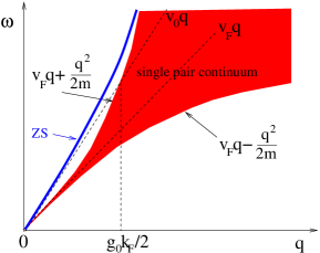
Figure 3: (Color online) Regime in the $\omega$-$q$ plane where $S_{\rm RPA}(\omega,q)$ is finite. The shaded regime represents the single-pair particle-hole continuum, while the thick line corresponds to the ZS mode. For weak interaction $g_{0}\ll 1$ the linear approximation $\omega_{q}\approx v_{0}|q|$ to the dispersion of the ZS mode crosses the upper boundary of the single-pair continuum at $q\approx g_{0}k_{F}/2$. However, the non-linear corrections to the ZS dispersion (LABEL:eq:dispersion) are such that it never intersects the single-pair continuum, so that there is no Landau damping.

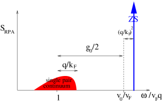
Figure 4: (Color online) Schematic behavior of $S_{\rm RPA}(\omega,q)$ for fixed $q\ll k_{F}$ as a function of $\omega$ for $q/k_{F}\ll g_{0}\ll 1$.In this regime, the distance between the upper edge of the single-pair particle-hole continuum and the position of the ZS peak (indicated by a thick arrow) is much larger than the width of the particle-hole continuum.

In the limit $g_{0}\rightarrow 0$ the ZS mode disappears and the incoherent part $S_{\rm RPA}^{\rm inc}(\omega,q)$ reduces to the dynamic structure factor of the free Fermi gas, which in one dimension for $q<2k_{F}$ is simply a box-function of width $q^{2}/m$ centered around $v_{F}|q|$,

$$S_{0}(\omega,q) = \lim_{g_{0}\rightarrow 0}S_{\rm RPA}^{\rm inc}(\omega,q)$$ (27)

$$= \frac{m}{2\pi|q|}\Theta\left(\frac{q^{2}}{2m}-\bigl{|}\omega-v_{F}|q|\bigr{|}\right).$$

For finite $g_{0}$, the shape of $S_{\rm RPA}^{\rm inc}(\omega,q)$ is modified as shown quantitatively in Fig. 1 of Ref. [Pirooznia07, ]. The small shaded hump in Fig. 4 represents schematically the incoherent part of $S_{\rm RPA}(\omega,q)$ for finite $g_{0}$. For $|q|/k_{F}\ll g_{0}$, the relative weight of the single-pair continuum is negligibly small, so that the ZS peak carries most of the spectral weight. For example, the relative contribution of the single-pair continuum to the $f$-sum rule vanishes as $(q/g_{0}k_{F})^{2}\ll 1$.

It is instructive to see which features of $S_{\rm RPA}(\omega,q)$ are recovered if we expand the inverse non-interacting polarization $\Pi_{0}^{-1}(Q)$ in powers of the inverse mass $m^{-1}$. Therefore we introduce the dimensionless variables,

$$iy = \frac{i\omega}{v_{F}q}\;,\;p=\frac{q}{2k_{F}},$$ (28)

and rewrite Eq. (21) as

$$\Pi_{0}(i\omega,q)=\nu_{0}\tilde{\Pi}_{0}(iy,p),$$ (29)

with the dimensionless function

$$\tilde{\Pi}_{0}(iy,p) = \frac{1}{2p}\ln\left|\frac{iy+1+p}{iy+1-p}\right|$$ (30)

$$= \frac{1}{4p}\ln\left[\frac{y^{2}+(1+p)^{2}}{y^{2}+(1-p)^{2}}\right].$$

For an interaction with momentum-transfer cutoff $q_{0}\ll k_{F}$ the relevant dimensionless momenta satisfy $|p|\ll 1$, so that we expand $\tilde{\Pi}^{-1}_{0}(iy,p)$ in powers of $p$. From Eq. (30) we find

$$\tilde{\Pi}_{0}^{-1}(iy,p)=1+y^{2}-\frac{p^{2}}{3}\frac{1-3y^{2}}{1+y^{2}}+O(p^{4}).$$ (31)

For later reference, we note that the correction of order $p^{2}$ in Eq. (31) can be written as

$$-\frac{p^{2}}{3}\frac{1-3y^{2}}{(1+y^{2})} = p^{2}\left[1-\frac{4}{3(1+y^{2})}\right]$$ (32)

$$=p^{2}-\frac{2p^{2}}{3}\left[\frac{1}{1-iy}+\frac{1}{1+iy}\right].$$

For $p\rightarrow 0$ we recover the result for linearized dispersion,

$$\lim_{p\rightarrow 0}\tilde{\Pi}^{-1}_{0}(iy,p)\equiv\tilde{\Pi}_{0}^{-1}(iy)=1+y^{2},$$ (33)

which yields the dynamic structure factor of the TLM given in Eq. (2). However, after analytic continuation to real frequencies $iy\rightarrow x+i0=\frac{\omega}{v_{F}q}+i0$, the correction term of order $p^{2}$ in the expansion (31) is singular on the mass-shell $|\omega|=v_{F}|q|$. Although in the non-interacting limit we know that this mass-shell singularity has been artificially generated by expanding the logarithm in Eq. (30), it is not at all obvious how to regularize a similar singularity if it is encountered in the interacting system. This is the reason why a formal expansion in powers of the band curvature $1/m$ using either a purely fermionic approach Teber06 or conventional bosonization Aristov07 is not reliable close to the mass-shell after analytic continuation. Fortunately, within the functional bosonization approach used in this work this problem does not arise, because the effective expansion parameter in functional bosonization is not $1/m$, but the combination $g_{0}q_{0}/(mv_{F})$, see Refs. [Kopietz95, ; Kopietz97, ]. In particular, in the non-interacting limit functional bosonization yields the exact structure factor of the free Fermi gas with quadratic dispersion, containing all orders in $1/m$.

It is instructive to examine the RPA dynamic structure factor if we nevertheless use the expansion (31) for the non-interacting polarization. Then we obtain after analytic continuation $iy\rightarrow x+i0=\omega/(v_{F}q)+i0$ for small $|q|\ll g_{0}k_{F}$,

$$S_{\rm RPA}(\omega,q) \approx \frac{\nu_{0}}{\pi}{\rm Im}\left[\frac{1}{g_{0}+\tilde{\Pi}^{-1}_{0}(x+i0,p)}\right]$$ (34)

$$=Z_{q}^{+}\delta(\omega-\tilde{\omega}_{q}^{+})+Z_{q}^{-}\delta(\omega-\tilde{\omega}_{q}^{-})\,,$$

where $Z_{q}^{+}$ and $\tilde{\omega}_{q}^{+}$ reduce for small $q$ to the corresponding expressions $Z_{q}$ and $v_{0}|q|$ for linear dispersion [see Eq. (4)], and the weight and dispersion of the other mode $\tilde{\omega}_{q}^{-}$ is for $|q|\ll k_{F}g_{0}$,

$$Z_{q}^{-}\approx\frac{2|q|}{3\pi}\left[\frac{q}{2k_{F}g_{0}}\right]^{2},$$ (35)

$$\tilde{\omega}_{q}^{-}\approx v_{F}|q|\left[1-\frac{2}{3g_{0}}\left(\frac{q}{2k_{F}}\right)^{2}\right]\,.$$ (36)

This peak is associated with the incoherent part $S_{\rm RPA}^{\rm inc}(\omega,q)$ of the dynamic structure factor discussed above, which in the approximation (31) is replaced by a single peak with the same weight. From Eqs. (35) and (4) one easily verifies that for $|q|\ll g_{0}k_{F}$ the relative weight of the peak associated with the incoherent part is indeed small,

$$\frac{Z_{q}^{-}}{Z_{q}^{+}}=\frac{4x_{0}}{3}\left[\frac{q}{2k_{F}g_{0}}\right]^{2}=\frac{4\pi^{2}x_{0}p_{0}^{2}}{3}\left[\frac{v_{F}q}{f_{0}q_{0}}\right]^{2}\,,$$ (37)

where we have used $p_{0}=q_{0}/(2k_{F})$, see Eqs. (14). Hence, for $|q|\ll g_{0}k_{F}$ most of the weight of $S_{\rm RPA}(\omega,q)$ is carried by the ZS mode $\tilde{\omega}_{q}^{+}\approx v_{0}|q|$, so that the incoherent part corresponding to the mode $\tilde{\omega}_{q}^{-}\approx v_{F}|q|$ can be neglected Pirooznia07 . Note that the limits $q\rightarrow 0$ and $g_{0}\rightarrow 0$ do not commute and that only for $|q|/(2k_{F})\ll g_{0}$ the weight of the mode $\tilde{\omega}_{q}^{-}$ can be neglected.

Mathematically, the second peak in Eq. (34) is due to the pole arising from the term of order $p^{2}$ in the expansion (31) of the inverse free polarization. Although after analytic continuation $iy\rightarrow x+i0$ this term is singular for $x=1$, we know from the exact result (30) how this singularity should be regularized: we simply should smooth out the corresponding $\delta$-function peak over an interval of width $\text{w}_{q}\propto q^{2}/m$. In fact, we can self-consistently calculate $\text{w}_{q}$ by noting that after analytic continuation the singular term in the expansion (31) gives rise to the following formally infinite imaginary part of the inverse non-interacting polarization,

$${\rm Im}\tilde{\Pi}_{0}^{-1}(x+i0,p)=-\Gamma_{0}(x,p)=-\frac{2\pi}{3}p^{2}[\delta(1-x)-\delta(1+x)].$$ (38)

Ignoring the renormalization arising from the (singular) real part of $\tilde{\Pi}_{0}^{-1}(x+i0,p)$ and approximating the resulting dynamic structure factor in this regime by a Lorentzian centered at $\omega=v_{F}|q|$, we find for the full width at half maximum in the limit $g_{0}\ll 1$,

$$\text{w}_{q}=\frac{v_{F}|q|}{2}\Gamma_{0}(1,p=q/(2k_{F})).$$ (39)

To obtain a self-consistent estimate for $\text{w}_{q}$ we follow Samokhin Samokhin98 and regularize the singularity in $\Gamma_{0}(1,p)$ by replacing $\delta(\omega=0)$ by the height of a normalized Lorentzian of width $\text{w}_{q}$ on resonance,

$$\left.\delta(x-1)\right|_{x=1}=v_{F}|q|\left.\delta(\omega-v_{F}|q|)\right|_{\omega=v_{F}|q|}\rightarrow\frac{v_{F}|q|}{\pi\text{w}_{q}}.$$ (40)

Hence, our self-consistent regularization is

$$\Gamma_{0}(1,p)\rightarrow\frac{2p^{2}v_{F}|q|}{3\text{w}_{q}}.$$ (41)

Substituting this into Eq. (39) we obtain the self-consistency equation

$$\text{w}_{q}=\frac{1}{3}\left(\frac{q}{2k_{F}}\right)^{2}\frac{(v_{F}q)^{2}}{\text{w}_{q}},$$ (42)

which leads to the following estimate for the width of the single-pair particle-hole continuum,

$$\text{w}_{q}=\frac{1}{2\sqrt{3}}\frac{q^{2}}{m}.$$ (43)

Of course, it is now known Pustilnik06 ; Pereira06 ; Pereira07 that the shape of the single-pair continuum cannot be approximated by a Lorentzian, but the order of magnitude of its width obtained within the above regularization is correct for sufficiently small $q$. Hence, the mass-shell singularity arising after analytic continuation $iy\rightarrow x+i0$ in the expansion of the inverse non-interacting polarization (31) in powers of $p=q/(2k_{F})$ is simply related to the single-pair particle-hole continuum. This singularity can be regularized by smearing out the $\delta$-function in the imaginary part over a finite interval of width $\text{w}_{q}\propto q^{2}/m$. However, the width $\text{w}_{q}$ should not be confused with the damping of the ZS mode, which remains sharp within RPA.

In order to obtain the ZS damping, one should calculate interaction corrections to the irreducible polarization. The finite overlap between the continuum due to particle-hole excitations involving more than a single particle-hole pair (multi-pair excitations) then determines the ZS damping. In three dimensions general phase space arguments Pines89 imply that the resulting damping is very small. In one dimension, an argument due to Teber Teber06 suggests that the damping of any acoustic collective mode which overlaps with the two-pair continuum should vanish as $q^{3}$ for small $q$. However, for this argument to be valid, one should self-consistently calculate the renormalized energy of the ZS mode and show that it is immersed in the multi-pair continuum. This has neither been done in our previous work Pirooznia07 , nor in the work by Pustilnik et al. Pustilnik06 , where the renormalization of the ZS velocity has been ignored.

In this work we shall carefully examine all corrections to the RPA to second order in an expansion in powers of the small parameter $p_{0}=q_{0}/(2k_{F})$, which is naturally generated using the functional bosonization approach Kopietz95 ; Kopietz97 . Most importantly, our approach does not suffer from the mass-shell singularities discussed above. Moreover, we shall show that the distinction between the ZS energy $v_{0}|q|$ and the energy scale $v_{F}|q|$ associated with the single-pair continuum shown schematically in Figs. 3 and 4 is an unphysical artefact of the RPA, which disappears once the corrections to the RPA are self-consistently taken into account.

III Functional bosonization

In this section we outline the functional bosonization approach Kopietz95 ; Kopietz96 ; Kopietz97 which we then use in Sec. IV to calculate the dynamic structure factor. In contrast to Refs. [Kopietz95, ; Kopietz96, ; Kopietz97, ], we shall here keep track of Hartree corrections to the fermionic self-energy, because these corrections contribute to the renormalization of the ZS velocity.

Decoupling the density-density interaction in Eq. (8) by means of a real Hubbard-Stratonovich field $\phi$, the ratio of the partition functions with and without interaction can be written as

$$\frac{\cal{Z}}{{\cal{Z}}_{0}}=\frac{\int{\cal{D}}[\bar{c},c,\phi]e^{-S_{0}[\bar{c},c]-S_{0}[\phi]-S_{1}[\bar{c},c,\phi]}}{\int{\cal{D}}[\bar{c},c,\phi]e^{-S_{0}[\bar{c},c]-S_{0}[\phi]}}\;,$$ (44)

where the free fermionic action $S_{0}[\bar{c},c]$ is given in Eq. (9), the free bosonic part is

$$S_{0}[\phi]=\frac{1}{2}\int_{Q}f^{-1}_{q}{\phi}_{-Q}\phi_{Q}\;,$$ (45)

and the Fermi-Bose interaction is

$$S_{1}[\bar{c},c,\phi] = i\int_{Q}\int_{K}\bar{c}_{K+Q}c_{K}\phi_{Q}.$$ (46)

The fermionic part of the action in the numerator of Eq. (44) can be written as

$$S_{0}[\bar{c},c]+S_{1}[\bar{c},c,\phi] = -\int_{K}\int_{K^{\prime}}\bar{c}_{K}[{\bf{G}}^{-1}]_{KK^{\prime}}{c}_{K^{\prime}},$$

where the infinite matrix ${\bf{G}}^{-1}$ is defined by

$$[{\bf{G}}^{-1}]_{KK^{\prime}}=\delta_{K,K^{\prime}}[i\omega-\epsilon_{k}+\mu]-i\phi_{K-K^{\prime}}.$$ (48)

At finite density, the field $\phi_{K}$ has a non-zero expectation value,

$$\phi_{Q}=-i\delta_{Q,0}\bar{\phi}+\delta\phi_{Q}.$$ (49)

Here the $\delta$-symbol is for finite $\beta$ and $V$ (where the components of $Q=(\bar{\omega},q)$ are discrete) given by $\delta_{Q,0}=\beta V\delta_{\bar{\omega},0}\delta_{q,0}$, which reduces to $(2\pi)^{2}\delta(\bar{\omega})\delta(q)$ for $\beta\rightarrow\infty$ and $V\rightarrow\infty$. We fix the real constant $\bar{\phi}$ from the requirement that the effective action $S_{\rm eff}[\phi]$ of the $\phi$-field, which is obtained by integrating over the fermionic fields in Eq. (44), does not contain a term linear in the fluctuation $\delta\phi_{Q}$. To do this, we define the matrix ${\bf{G}}_{0}^{-1}$ which includes the self-energy correction due to the vacuum expectation value $\bar{\phi}$,

$$[{\bf{G}}_{0}^{-1}]_{KK^{\prime}}=\delta_{K,K^{\prime}}[i\omega-\epsilon_{k}-\bar{\phi}+\mu],$$ (50)

and write

$${\bf{G}}^{-1}={\bf{G}}_{0}^{-1}-{\bf{V}},$$ (51)

with

$$[{\bf{V}}]_{KK^{\prime}}=i\delta\phi_{K-K^{\prime}}.$$ (52)

Integrating in Eq. (44) over the fermion fields we obtain the formally exact expression

$$\frac{\cal{Z}}{{\cal{Z}}_{0}}=e^{-\beta(\Omega_{1}-\Omega_{0})}\frac{\int{\cal{D}}[\delta\phi]e^{-S_{\rm eff}[\delta\phi]}}{\int{\cal{D}}[\phi]e^{-S_{0}[\phi]}}\;,$$ (53)

where $\Omega_{1}-\Omega_{0}$ is the change of the grand canonical potential due to the vacuum expectation value ignoring fluctuations,

$$\Omega_{1}-\Omega_{0}=\frac{1}{\beta}{\rm Tr}\ln[\mathbf{G}_{0}(\bar{\phi})\mathbf{G}^{-1}_{0}(\bar{\phi}=0)]-V\frac{\bar{\phi}^{2}}{2f_{0}}.$$ (54)

The effective action for the fluctuations of the bosonic field is

$$S_{\rm eff}[\delta\phi] = S_{0}[\phi_{Q}\rightarrow-i\delta_{Q,0}\bar{\phi}+\delta\phi_{Q}]-\beta V\frac{\bar{\phi}^{2}}{2f_{0}}$$ (55)

$$-{\rm Tr}\ln[1-{\bf{G}}_{0}\bm{V}]$$

$$= \frac{1}{2}\int_{Q}f_{q}^{-1}\delta\phi_{-Q}\delta\phi_{Q}-if_{0}^{-1}\bar{\phi}\delta\phi_{0}$$

$$+\sum_{n=1}^{\infty}\frac{{\rm Tr}[{\bf{G}}_{0}\bm{V}]^{n}}{n}.$$

We now fix the vaccum expectation value $\bar{\phi}$ from the saddle point condition

$$\frac{\partial\Omega_{1}}{\partial\bar{\phi}}=-V\frac{\bar{\phi}}{f_{0}}+V\rho_{0}=0,$$ (56)

or equivalently

$$\bar{\phi}=f_{0}\rho_{0}.$$ (57)

Here, $\rho_{0}$ is the density and $G_{0}(K)$ is the fermionic Green function in self-consistent Hartree approximation, where

$$\rho_{0}=\int_{K}G_{0}(K)=\frac{1}{V}\sum_{k}\Theta(\mu-\epsilon_{k}-f_{0}\rho_{0})\,,$$ (58)

$$G_{0}(K)=\frac{1}{i\omega-\epsilon_{k}-f_{0}\rho_{0}+\mu}.$$ (59)

Note that Eq. (59) agrees with Eq. (19) if we take into account that within self-consistent Hartree approximation the Fermi momentum $k_{F}$ is defined via

$$\frac{k_{F}^{2}}{2m}=\mu-f_{0}\rho_{0}.$$ (60)

Eq. (56) guarantees that the terms linear in the fluctuations $\delta\phi_{Q}$ in Eq. (55) cancel, so that our final result for the effective action for the fluctuations of the Hubbard-Stratonovich field is

$$S_{\rm eff}[\delta\phi] = \frac{1}{2}\int_{Q}f_{q}^{-1}\delta\phi_{-Q}\delta\phi_{Q}+\sum_{n=2}^{\infty}\frac{{\rm Tr}[{\bf{G}}_{0}\bm{V}]^{n}}{n}$$ (61)

$$= S_{2}[\delta\phi]+S_{\rm int}[\delta\phi],$$

with the Gaussian part given by

$$S_{2}[\delta\phi]=\frac{1}{2}\int_{Q}[f_{q}^{-1}+\Pi_{0}(Q)]\delta\phi_{-Q}\delta\phi_{Q},$$ (62)

and the interaction part

$$S_{\rm int}[\delta\phi] = \sum_{n=3}^{\infty}\frac{1}{n!}\int_{Q_{1}}\ldots\int_{Q_{n}}\delta_{Q_{1}+\ldots+Q_{n},0}$$ (63)

$$\times \Gamma_{0}^{(n)}(Q_{1},\ldots,Q_{n})\delta\phi_{Q_{1}}\ldots\delta\phi_{Q_{n}}.$$

The vertices $\Gamma_{0}^{(n)}(Q_{1},\ldots,Q_{n})$ are proportional to the symmetrized closed fermion loops $L^{(n)}_{S}(Q_{1},\ldots,Q_{n})$ defined in Eq. (174),

$$\Gamma^{(n)}_{0}(Q_{1},\ldots,Q_{n}) = i^{n}(n-1)!L^{(n)}_{S}(-Q_{1},\ldots,-Q_{n}).$$

A graphical representation of $\Gamma^{(n)}_{0}(Q_{1},\ldots,Q_{n})$ is shown in Fig. 5.

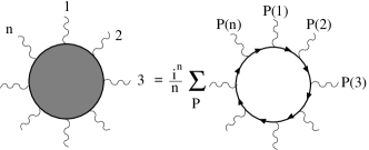
Figure 5: Boson vertex with $n$ external legs in the interaction part $S_{\rm int}[\delta\phi]$ of the bosonized effective action, see Eq. (63). The arrows denote the fermionic Green functions $G_{0}(K)$ within self-consistent Hartree approximation, see Eq. (59). The sum is taken over the $n!$ permutations of the labels of the external legs. For linearized energy dispersion all symmetrized closed fermion loops with more than two external legs vanish.

In appendix A we give explicit expressions for the symmetrized $n$-loops of the FSM Neumayr98 ; Neumayr99 ; Kopper01 and show that $L_{S}^{(n)}\propto(1/m)^{n-2}$ to leading order in $1/m$. Moreover, in appendices B and C we carefully discuss the properties of the loops $L_{S}^{(3)}(Q_{1},Q_{2},-Q_{1}-Q_{2})$ and $L_{S}^{(4)}(Q_{1},Q_{2},-Q_{1},-Q_{2})$ for the special combinations of momenta needed in this work.

The exact irreducible polarization can now be obtained from the fluctuation propagator of the Hubbard-Stratonovich field,

$$\langle\delta\phi_{Q}\delta\phi_{Q^{\prime}}\rangle = \frac{\int{\cal{D}}[\delta\phi]e^{-S_{\rm eff}[\delta\phi]}\delta\phi_{Q}\delta\phi_{Q^{\prime}}}{\int{\cal{D}}[\delta\phi]e^{-S_{\rm eff}[\delta\phi]}}$$ (65)

$$= \delta_{Q+Q^{\prime},0}\frac{1}{f_{q}^{-1}+\Pi_{\ast}(Q)},$$

where the effective action $S_{\rm eff}[\delta\phi]$ is defined in Eq. (61). Within the Gaussian approximation this reduces to the RPA interaction

$$\langle\delta\phi_{Q}\delta\phi_{Q^{\prime}}\rangle_{S_{2}} = \delta_{Q+Q^{\prime},0}\frac{1}{f_{q}^{-1}+\Pi_{0}(Q)}$$ (66)

$$\equiv \delta_{Q+Q^{\prime},0}f_{\rm RPA}(Q).$$

The corrections to the RPA can now be calculated systematically in powers of the interaction $S_{\rm int}$ using the Wick theorem. The RPA interaction thereby plays the role of the Gaussian propagator, so that we naturally obtain an expansion in powers of the RPA interaction. As discussed in appendix A, the vertices $\Gamma^{(n)}_{0}(Q_{1},\ldots,Q_{n})$ with $n$ external bosonic legs are proportional to $(1/m)^{n-2}$, so that the underlying small parameter of our expansion is the product of the RPA interaction and $1/m$. In particular, in the limit of vanishing interaction we recover the exact non-interacting polarization $\Pi_{0}(i\omega,q)$ for quadratic energy dispersion. Our approach based on functional bosonization is therefore fundamentally different from conventional bosonization Samokhin98 ; Teber06 ; Aristov07 , where the quadratic term in the energy dispersion gives rise to a cubic vertex proportional to $1/m$ which has to be re-summed to infinite order to recover the correct non-interacting polarization.

IV Calculation of $S(\omega,q)$ using functional bosonization

IV.1 One-loop self-consistency equation for $\Pi_{\ast}(Q)$

It is now straightforward to expand the irreducible polarization in powers of the RPA interaction, which is the Gaussian propagator of our boson field $\delta\phi_{Q}$. The diagrams contributing to $\Pi_{\ast}(Q)$ up to second order in the RPA interaction are shown in Fig. 6.

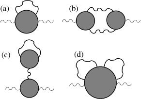
Figure 6: Diagrams arising in the perturbative expansion of the irreducible polarization to second order in the RPA interaction. The shaded circles represent the vertices of $S_{\rm eff}[\delta\phi]$, which are related to symmetrized closed fermion loops as defined in Fig. 5. Diagram (a) is equivalent to the three fermionic diagrams shown in Fig. 2. Diagram (b) is the so-called Aslamazov-Larkin diagram, while diagram (c) can be viewed as a higher order self-energy correction which renormalizes the relation between density and chemical potential. Diagram (d) involving two bosonic loops and the symmetrized fermionic six-loop is of fourth order in $p_{0}=q_{0}/(2k_{F})$ and can be neglected to order $p_{0}^{2}$.

The relevant dimensionless parameter for this expansion is the ratio $p_{0}=q_{0}/(2k_{F})$, because by assumption the range of the interaction in momentum space has a cutoff $q_{0}\ll k_{F}$ so that each additional bosonic loop integration gives rise to a factor of $p_{0}^{2}$. Hence, the diagram (d) involving two bosonic loops of is of order $p_{0}^{4}$, because according to Eq. (189) the symmetrized fermion loop with six external legs is proportional to $1/m^{4}$ and the two bosonic loop integrations generate a factor of $q_{0}^{4}$. Because the other three diagrams are proportional to $p_{0}^{2}$, it is consistent to neglect diagram (d) as long as we retain all terms up to order $p_{0}^{2}$. Evaluating the diagrams (a)–(c) in Fig. 6 we obtain the following expression for the irreducible polarization,

$$\Pi_{\ast}(Q) \approx \Pi_{0}(Q)-\frac{1}{2}\int_{{Q^{\prime}}}{f}_{\rm RPA}({Q}^{\prime})\Biggl{\{}6L^{(4)}_{S}({Q}^{\prime},-{Q}^{\prime},{Q},-Q)+4{f}_{\rm RPA}(0)L^{(3)}_{S}(Q,-Q,0)L^{(3)}_{S}({Q}^{\prime},-{Q}^{\prime},0)$$ (67)

$$\hskip 113.81102pt+4f_{\rm RPA}(Q+{Q}^{\prime})L^{(3)}_{S}(-{Q},{Q}+{Q}^{\prime},-{Q}^{\prime})L^{(3)}_{S}({Q}^{\prime},-{Q}-{Q}^{\prime},{Q})\Biggl{\}}.$$

The properties of the symmetrized three- and four-loops appearing in this expression are discussed in detail in appendices B and C. It turns out, however, that in order to cure the unphysical features of the RPA discussed at the end of Sec. II (in particular, within RPA the energy scale $v_{F}|q|$ of the single-pair continuum erroneously involves the bare Fermi velocity), we should self-consistently dress the Gaussian propagator $f_{\rm RPA}(Q)$ in Eq. (67) by self-energy corrections. Formally, this amounts to replacing the RPA interaction by the exact effective interaction,

$$f_{\rm RPA}(Q)\rightarrow f_{\ast}(Q)=\frac{f_{q}}{1+f_{q}\Pi_{\ast}(Q)}.$$ (68)

In appendix D we justify this procedure using a functional renormalization group approach Schuetz05 ; Schuetz06 . With this substitution, Eq. (67) becomes a complicated integral equation for the irreducible polarization, which cannot be solved analytically. Fortunately, this integral equation can again be simplified by noting that on the right-hand side it is not necessary to retain the full $Q$-dependence of $\Pi_{\ast}(Q)$, but to keep only those terms which contribute to the self-consistent renormalization of the ZS velocity. To explain this, let us introduce again the dimensionless variables $iy=i\omega/(v_{F}q)$ and $p=q/(2k_{F})$ and define the dimensionless irreducible polarization

$$\Pi_{\ast}(i\omega,q)=\nu_{0}\tilde{\Pi}_{\ast}(iy,p).$$ (69)

The corresponding dimensionless effective interaction is then

$$\tilde{f}_{\ast}(iy,p)=\frac{g_{p}}{1+g_{p}\tilde{\Pi}_{\ast}(iy,p)},$$ (70)

where $g_{p}=\nu_{0}f_{q=pk_{F}}$, see also Eqs. (28) and (29). The dynamic structure factor can then be written as

$$S(\omega,q) = \frac{1}{\pi}{\rm Im}\left[\frac{1}{f_{q}+\Pi_{\ast}^{-1}(\omega+i0,q)}\right]$$ (71)

$$= \frac{\nu_{0}}{\pi}{\rm Im}\left[\frac{1}{g_{p}+\tilde{\Pi}_{\ast}^{-1}(x+i0,p)}\right],$$

where $x=\omega/(v_{F}q)$. For our purpose it is now sufficient to approximate the dimensionless inverse irreducible polarization by

$$\tilde{\Pi}_{\ast}^{-1}(iy,p)=Z_{1}+Z_{2}y^{2},$$ (72)

where the dimensionless renormalization factors $Z_{1}$ and $Z_{2}$ should be determined as a function of the interaction such that the approximation (72) yields the true ZS velocity $v$. Within RPA, where the non-linear terms in the energy dispersion do not renormalize the ZS velocity, the irreducible polarization is approximated by the non-interacting one, so that $Z_{1}=Z_{2}=1$. If we approximate the inverse polarization in Eq. (71) by Eq. (72) we obtain for $\omega>0$ and $q\rightarrow 0$,

$$S(\omega,q)\approx\frac{v_{F}|q|}{2\pi vZ_{2}}\delta(\omega-v|q|),$$ (73)

where the renormalized ZS velocity is

$$\frac{v}{v_{F}}=\sqrt{\frac{Z_{1}+g_{0}}{Z_{2}}}\equiv x_{0}\equiv\sqrt{1+g},$$ (74)

with renormalized coupling constant

$$g=\frac{g_{0}+Z_{1}}{Z_{2}}-1.$$ (75)

In order to avoid the unphysical splitting of the spectral weight in $S(\omega,q)$ (as discussed at the end of Sec. II, this is an artefact of the RPA) it is crucial that the true ZS velocity $v$ appears in the bosonic propagators. Therefore, a naive expansion in powers of the RPA interaction is not sufficient. However, we may further reduce the complexity of the calculation by noting that Eq. (73) still contains the correct velocity if we set $Z_{2}\rightarrow 1$ in the prefactor. Within this approximation, the velocity renormalization implied by Eq. (72) can be simply taken into account via a re-definition of the coupling constant, $g_{0}\rightarrow g$. It is therefore sufficient to replace the RPA interaction in Eq. (67) by an effective interaction of the same form but with a renormalized effective coupling $g$ instead of $g_{0}$, which should be chosen such that all interaction corrections to the ZS velocity are self-consistently taken into account. Note that Schönhammer Schoenhammer07 has recently shown that within the so-called RPAE approximation (which amounts to solving the Bethe-Salpeter equation with the bare interaction as irreducible vertex) the relative position of the collective mode energy and the energy of the single-pair particle-hole continuum is different from the RPA prediction for the FSM: In RPAE the ZS mode lies above the non-interacting single particle-hole continuum which (erroneously) appears in RPA, but below the Hartree-Fock particle-hole continuum. This suggests that in order to obtain a correct estimate of the ZS damping, it is necessary to calculate the location of the ZS energy self-consistently.

In field-theoretical language the constants $Z_{1}$ and $Z_{2}$ are counter-terms which guarantee that our Gaussian propagator depends on the true ZS velocity. In Sec. V we shall explicitly calculate the factors $Z_{1}$, $Z_{2}$ and the corresponding renormalized ZS velocity $v$ to second order in our small parameter $p_{0}$. A similar procedure is necessary to self-consistently calculate the true Fermi surface of an interacting Fermi system Neumayr03 ; Ledowski03 . The expansion of the modified dimensionless interaction $\tilde{g}_{p}$ for small $p$ is then

$$\tilde{g}_{p}=g+\frac{1}{2}g_{0}^{\prime\prime}p^{2}+O(p^{4}),$$ (76)

where

$$g_{0}^{\prime\prime}=(2k_{F})^{2}\nu_{0}f_{0}^{\prime\prime}={\rm sign}f_{0}^{\prime\prime}\frac{2}{\pi p_{c}}.$$ (77)

In this approximation, our dimensionless effective interaction is

$$\tilde{f}_{\ast}(iy,p)\approx\tilde{f}_{g}(iy,p)=\frac{\tilde{g}_{p}}{1+\tilde{g}_{p}\tilde{\Pi}_{0}(iy,p)},$$ (78)

which differs from the RPA interaction, because the function $\tilde{g}_{p}$ includes the renormalization of the ZS velocity due to fluctuations beyond the RPA.

Collecting all terms, our final result for the dimensionless irreducible polarization to one bosonic loop can be written as

$$\tilde{\Pi}_{\ast}(iy,p)\approx\tilde{\Pi}_{0}(iy,p)+\tilde{\Pi}_{1}(iy,p)+\tilde{\Pi}_{2}(iy,p),$$ (79)

where the non-interacting polarization is given in Eq. (30), and the subscripts indicate the powers of $\tilde{g}_{p}$. The term $\tilde{\Pi}_{1}(iy,p)$ corresponding to diagram (a) in Fig. 6 can be written as

$$\tilde{\Pi}_{1}(iy,p) = -\int_{-\infty}^{\infty}dp^{\prime}|p^{\prime}|\int_{-\infty}^{\infty}\frac{dy^{\prime}}{2\pi}\tilde{f}_{g}(iy^{\prime},p^{\prime})\tilde{L}^{(4)}_{S}(iy,p,iy^{\prime},p^{\prime}),$$ (80)

where the dimensionless symmetrized four-loop $\tilde{L}^{(4)}_{S}(iy,p,iy^{\prime},p^{\prime})$ is defined in Eq. (206). The term $\tilde{\Pi}_{2}(iy,p)$ involving two powers of the effective interaction is of the form

$$\tilde{\Pi}_{2}(iy,p)=\tilde{\Pi}_{2}^{\rm AL}(iy,p)+\tilde{\Pi}_{2}^{\rm H}(iy,p),$$ (81)

where the contribution from the Aslamasov-Larkin (AL) diagram in Fig. 6 (b) is

$$\tilde{\Pi}_{2}^{\rm AL}(iy,p) = -\int_{-\infty}^{\infty}dp^{\prime}|p^{\prime}|\int_{-\infty}^{\infty}\frac{dy^{\prime}}{2\pi}\tilde{f}_{g}(iy^{\prime},p^{\prime})\tilde{f}_{g}\left(\frac{iyp+iy^{\prime}p^{\prime}}{p+p^{\prime}},p+p^{\prime}\right)[\tilde{L}^{(3)}_{S}(iy,p,iy^{\prime},p^{\prime})]^{2},$$ (82)

and the contribution from the Hartree diagram in Fig. 6 (c) can be written as

$$\tilde{\Pi}_{2}^{\rm H}(iy,p) = -\frac{g}{1+g}\tilde{L}^{(3)}_{S}(iy,p,iy,-p)\int_{-\infty}^{\infty}dp^{\prime}|p^{\prime}|\int_{-\infty}^{\infty}\frac{dy^{\prime}}{2\pi}\tilde{f}_{g}(iy^{\prime},p^{\prime})\tilde{L}^{(3)}_{S}(iy^{\prime},p^{\prime},iy^{\prime},-p^{\prime}).$$ (83)

Here, the dimensionless symmetrized three-loop $\tilde{L}^{(3)}_{S}(iy,p,iy^{\prime},p^{\prime})$ is defined in Eq. (192). The parameters $Z_{1}$ and $Z_{2}$ hidden in the effective interaction $\tilde{f}_{g}(iy,p)$ should be determined self-consistently by evaluating Eqs.(79–83) and demanding that the resulting renormalized ZS velocity is consistent with the result obtained from Eq. (72). We emphasize again that the above expression for $\Pi_{\ast}(Q)$ is not based on an expansion in powers of $1/m$: all functions appearing in Eqs. (80–83) depend on $1/m$ in a rather complicated non-linear manner.

IV.2 Approximation A: neglecting $1/m$-corrections to $\Pi_{0}(Q)$ in loop integrations

Eqs. (80–83) are still too complicated to admit an analytic evaluation. In order to explicitly calculate the dynamic structure factor without resorting to elaborate numerics, we shall further simplify the above expressions by making the following approximation A: We replace the non-interacting polarization $\Pi_{0}(Q)$ appearing in the effective interaction and the symmetrized closed fermion loops on the right-hand sides of Eqs. (80–83) by its asymptotic limit for small momenta given in Eq. (33). Keeping in mind that in one dimension the closed fermion loops with $n>2$ external legs can all be expressed in terms of $\Pi_{0}(Q)$, the symmetrized three- and four-loops are then approximated by Eqs. (197) and (211). For consistency, we should also expand the dimensionless free polarization $\tilde{\Pi}_{0}(iy,p)$ on the right-hand side of Eq. (79) to second order in $p$, see Eq. (31). We shall argue below that the above approximation A is not sufficient to calculate the line-shape of the dynamic structure factor for momenta $q\lesssim q_{c}=1/(m|f_{0}^{\prime\prime}|)$ [see Eq. (16)], because in this regime the spectral line-shape is dominated by the terms neglected in approximation A. On the other hand, for $q\gtrsim q_{c}$ the line-shape of $S(\omega,q)$ is essentially determined by the quadratic term in the expansion of $f_{q}$ for small $q$, so that in this regime A is justified.

It turns out that with this simplification the $y^{\prime}$-integrations in Eqs. (80), (82) and (83) can be done analytically for general $\tilde{g}_{p}$ using the method of residues. The form of Eq. (71) suggests that it is natural to expand the inverse irreducible polarization in powers of $p$ and $p_{0}$. This procedure can be formally justified within functional bosonization Kopietz97 ; Pirooznia07 , where the interaction corrections to the inverse irreducible polarization play the role of the self-energy corrections in the effective bosonized theory. But it is usually better to expand the self-energy rather than the Green function in powers of the relevant small parameter, because the direct expansion of the Green function usually leads to unphysical singularities. Using Eqs. (31) and (80–83) we obtain for the expansion of the inverse irreducible polarization to order $p_{0}^{2}$,

$$\tilde{\Pi}_{\ast}^{-1}(iy,p) = 1+y^{2}-\frac{p^{2}}{3}\frac{1-3y^{2}}{1+y^{2}}$$ (84)

$$- (1+y^{2})^{2}\tilde{\Pi}_{1}(iy,p)$$

$$- (1+y^{2})^{2}\tilde{\Pi}_{2}(iy,p)+O(p_{0}^{3}),$$

where $p$ is assumed to be smaller than the dimensionless momentum-transfer cutoff $p_{0}=q_{0}/(2k_{F})$. It is convenient to introduce the notation

$$x_{p} = \sqrt{1+\tilde{g}_{p}},$$ (85a)

$$a_{p} = x_{p}+1=\sqrt{1+\tilde{g}_{p}}+1,$$ (85b)

$$b_{p} = x_{p}-1=\sqrt{1+\tilde{g}_{p}}-1,$$ (85c)

so that $a_{p}b_{p}=\tilde{g}_{p}$. The contribution involving the symmetrized four-loop can then be written as

$$-(1+y^{2})^{2}\tilde{\Pi}_{1}(iy,p) = {\rm Re}\int_{0}^{\infty}dp^{\prime}\Biggl{\{}\frac{|p^{\prime}|}{x_{p^{\prime}}}\frac{p^{\prime 4}F_{1}(iy,p^{\prime})+p^{\prime 2}p^{2}F_{2}(iy,p^{\prime})+p^{4}F_{3}(iy,p^{\prime})}{[a_{p^{\prime}}^{2}p^{\prime 2}-(1+iy)^{2}p^{2}][b_{p^{\prime}}^{2}p^{\prime 2}-(1-iy)^{2}p^{2}]}$$ (86)

$$\hskip 34.1433pt-p^{\prime 2}\tilde{g}_{p^{\prime}}(1+iy)^{2}\Bigl{[}\frac{2p^{\prime}}{p(1-iy)}+1\Bigr{]}\frac{|p+p^{\prime}|}{x_{p^{\prime}}^{2}p^{\prime 2}-[(1-iy)p+p^{\prime}]^{2}}+(p^{\prime}\rightarrow-p^{\prime})\Biggr{\}},$$

with

$$F_{1}(iy,p) = 4\tilde{g}_{p}(x_{p}+iy)^{2}+\tilde{g}_{p}^{2}\left[\frac{8x_{p}}{1-iy}-4x_{p}-\tilde{g}_{p}-(2+x_{p}-\frac{\tilde{g}_{p}}{2})(1+y^{2})\right],$$ (87)

$$F_{2}(iy,p) = \tilde{g}_{p}\left[-(1+iy)^{4}+\tilde{g}_{p}(2-y^{2}+y^{4})-4b_{p}iy(1-y^{2})\right]-2b_{p}^{2}x_{p}\frac{1+iy}{1-iy}(3-6y^{2}-y^{4}),$$ (88)

$$F_{3}(iy,p) = -4b_{p}^{2}(1+y^{2})\left[1-\frac{1+y^{2}}{2}-\frac{(1+y^{2})^{2}}{8}\right].$$ (89)

Both functions $F_{1}(iy,p)$ and $F_{2}(iy,p)$ contain a singular term proportional to $(1-iy)^{-1}$, which after analytic continuation give rise to a mass-shell singularity at the energies $\pm v_{F}q$ associated with the bare Fermi velocity. Fortunately, these singularities cancel when Eq. (86) is combined with the corresponding contributions from the expansion of $\tilde{\Pi}_{0}^{-1}(iy,p)$ in Eq. (84) and from the AL diagram given in Eq. (96) below. To show this explicitly, it is useful to isolate the singular term in Eqs. (87) and (88) by setting

$$F_{1}(iy,p) = \frac{8\tilde{g}_{p}^{2}x_{p}}{1-iy}+\tilde{F}_{1}(iy,p),$$ (90)

$$F_{2}(iy,p) = -8b_{p}^{2}x_{p}\frac{(1+iy)^{2}}{1-iy}+\tilde{F}_{2}(iy,p).$$ (91)

$\tilde{F}_{1}(iy,p)$ and $\tilde{F}_{2}(iy,p)$ are now analytic functions of $y$,

$$\tilde{F}_{1}(iy,p) = 4\tilde{g}_{p}(x_{p}+iy)^{2}-\tilde{g}_{p}^{2}\left[4x_{p}+\tilde{g}_{p}+(2+x_{p}-\frac{\tilde{g}_{p}}{2})(1+y^{2})\right],$$ (92)

$$\tilde{F}_{2}(iy,p) = \tilde{g}_{p}\Bigl{[}-(1+iy)^{4}+\tilde{g}_{p}(2-y^{2}+y^{4})+4b_{p}iy(1+2iy+y^{2})\Bigr{]}$$ (93)

$$+ 2b_{p}^{2}(1+iy)\left[x_{p}(1+iy)(1+y^{2})-4iy\right].$$

Eq. (86) can then be written as

$$-(1+y^{2})^{2}\tilde{\Pi}_{1}(iy,p) = {\rm Re}\int_{0}^{\infty}dp^{\prime}\Biggl{\{}\frac{|p^{\prime}|}{x_{p^{\prime}}}\frac{p^{\prime 4}\tilde{F}_{1}(iy,p^{\prime})+p^{\prime 2}p^{2}\tilde{F}_{2}(iy,p^{\prime})+p^{4}F_{3}(iy,p^{\prime})}{[a_{p^{\prime}}^{2}p^{\prime 2}-(1+iy)^{2}p^{2}][b_{p^{\prime}}^{2}p^{\prime 2}-(1-iy)^{2}p^{2}]}+\frac{8|p^{\prime}|}{1-iy}+\frac{8|p^{\prime}|p^{2}(1-iy)}{b_{p^{\prime}}^{2}p^{\prime 2}-(1-iy)^{2}p^{2}}$$ (94)

$$\hskip 45.5244pt-p^{\prime 2}\tilde{g}_{p^{\prime}}(1+iy)^{2}\Bigl{[}\frac{2p^{\prime}}{p(1-iy)}+1\Bigr{]}\frac{|p^{\prime}+p|}{x_{p^{\prime}}^{2}p^{\prime 2}-[p^{\prime}+(1-iy)p]^{2}}+(p^{\prime}\rightarrow-p^{\prime})\Biggr{\}}.$$

Next, consider the contribution $\tilde{\Pi}_{2}^{\rm AL}(iy,p)$ from the Aslamasov-Larkin diagram in Eq. (82). Adopting again approximation A, the symmetrized three-loop $\tilde{L}^{(3)}_{S}(iy,p,iy^{\prime},p^{\prime})$ is replaced by its limit $\tilde{L}^{(3)}_{S,0}(iy,iy^{\prime},p/p^{\prime})$ for $1/m\rightarrow 0$ given in Eq. (197). Then we obtain

$$-(1+y^{2})^{2}\tilde{\Pi}_{2}^{\rm AL}(iy,p) = \int_{-\infty}^{\infty}dp^{\prime}|p^{\prime}|\tilde{g}_{p^{\prime}}\tilde{g}_{p^{\prime}+p}\int_{-\infty}^{\infty}\frac{dy^{\prime}}{2\pi}\frac{\left[1-yy^{\prime}-(y+y^{\prime})\frac{py+p^{\prime}y^{\prime}}{p+p^{\prime}}\right]^{2}}{\Bigl{[}1+y^{\prime 2}\Bigr{]}\Bigl{[}x_{p^{\prime}}^{2}+y^{\prime 2}\Bigr{]}\Bigl{[}1+\left(\frac{py+p^{\prime}y^{\prime}}{p+p^{\prime}}\right)^{2}\Bigr{]}\Bigl{[}x_{p^{\prime}+p}^{2}+\left(\frac{py+p^{\prime}y^{\prime}}{p+p^{\prime}}\right)^{2}\Bigr{]}}.$$

The $y^{\prime}$-integration can now be carried out using the theorem of residues. The result can be cast into the following form,

$$-(1+y^{2})^{2}\tilde{\Pi}_{2}^{\rm AL}(iy,p) = {\rm Re}\int_{0}^{\infty}dp^{\prime}p^{\prime}\frac{|p^{\prime}+p|}{2}\Biggl{\{}\frac{\tilde{g}_{p^{\prime}+p}|p^{\prime}+p|\Bigl{[}(p^{\prime}+p)(1+2iyx_{p^{\prime}}+x^{2}_{p^{\prime}})-p(y^{2}+x^{2}_{p^{\prime}})\Bigr{]}^{2}}{x_{p^{\prime}}\bigr{[}(p^{\prime}+p)^{2}-\bigr{(}x_{p^{\prime}}p^{\prime}+iyp\bigr{)}^{2}\bigl{]}\bigr{[}x_{p^{\prime}+p}^{2}(p^{\prime}+p)^{2}-\bigl{(}x_{p^{\prime}}p^{\prime}+iyp\bigr{)}^{2}\bigl{]}}$$ (96)

$$\hskip 91.04881pt+\frac{\tilde{g}_{p^{\prime}}p^{\prime}\Bigl{[}p^{\prime}(1+2iyx_{p^{\prime}+p}+x^{2}_{p^{\prime}+p})+p(y^{2}+x^{2}_{p^{\prime}+p})\Bigr{]}^{2}}{x_{p^{\prime}+p}\bigr{[}p^{\prime 2}-\bigr{(}x_{p^{\prime}+p}(p^{\prime}+p)-iyp\bigr{)}^{2}\bigl{]}\bigr{[}x_{p^{\prime}}^{2}p^{\prime 2}-\bigl{(}x_{p+p^{\prime}}(p+p^{\prime})-iyp\bigr{)}^{2}\bigl{]}}$$

$$\hskip 91.04881pt-\Bigl{[}\frac{2(p^{\prime}+p)}{p(1-iy)}-1\Bigr{]}\frac{\tilde{g}_{p^{\prime}+p}|p^{\prime}+p|(1+iy)^{2}}{x_{p^{\prime}+p}^{2}(p^{\prime}+p)^{2}-[p^{\prime}+p-(1-iy)p]^{2}}$$

$$\hskip 91.04881pt+\Bigl{[}\frac{2p^{\prime}}{p(1-iy)}+1\Bigr{]}\frac{\tilde{g}_{p^{\prime}}p^{\prime}(1+iy)^{2}}{x_{p^{\prime}}^{2}p^{\prime 2}-[p^{\prime}+(1-iy)p]^{2}}\Biggr{\}}+(p\rightarrow-p).$$

Finally, the contribution (83) of the Hartree-type-of diagram (c) in Fig. 6 is footnotehartree

$$-(1+y^{2})^{2}\tilde{\Pi}_{2}^{\rm H}(iy,p)=I_{H}(1-y^{2}),$$ (97)

with

$$I_{H} = -\frac{2g}{1+g}\int_{0}^{\infty}dpp\left[\frac{1+\frac{\tilde{g}_{p}}{2}}{\sqrt{1+\tilde{g}_{p}}}-1\right]$$ (98)

$$= -\frac{g}{1+g}\int_{0}^{\infty}dpp\frac{(x_{p}-1)^{2}}{x_{p}}.$$

For $\Theta$-function cutoff this reduces to

$$I_{H}=-\frac{p_{0}^{2}g}{1+g}\left[\frac{1+\frac{g}{2}}{\sqrt{1+g}}-1\right],$$ (99)

while for Lorentzian cutoff,

$$I_{H}=-\frac{p_{0}^{2}g}{1+g}\left[1+\frac{g}{2}-\sqrt{1+g}\right].$$ (100)

Combining all terms we obtain the following expansion of the inverse irreducible polarization to second order in $p_{0}^{2}$,

$$\tilde{\Pi}_{\ast}^{-1}(iy,p) = 1+y^{2}+p^{2}-\frac{2p^{2}}{3}\left[\frac{1}{1-iy}+\frac{1}{1+iy}\right]$$ (101)

$$+I_{H}(1-y^{2})+I(iy,p)+O(p_{0}^{3}),$$

where we have used Eqs. (31) and (32) to clearly exhibit the mass-shell singularity generated by the expansion of the inverse free polarization. The dimensionless integral $I(iy,p)$ can be written as

$$I(iy,p)=\frac{1}{2}\int_{0}^{\infty}dp^{\prime}p^{\prime}\left[J(iy,p,p^{\prime})+J(-iy,p,p^{\prime})\right],$$ (102)

where the complex function $J(iy,p,p^{\prime})$ is given by

$$J(iy,p,p^{\prime}) = \frac{p^{\prime 4}\tilde{F}_{1}(iy,p^{\prime})+p^{\prime 2}p^{2}\tilde{F}_{2}(iy,p^{\prime})+p^{4}F_{3}(iy,p^{\prime})}{x_{p^{\prime}}[a_{p^{\prime}}^{2}p^{\prime 2}-(1+iy)^{2}p^{2}][b_{p^{\prime}}^{2}p^{\prime 2}-(1-iy)^{2}p^{2}]}+\frac{8}{1-iy}+\frac{8p^{2}(1-iy)}{b_{p^{\prime}}^{2}p^{\prime 2}-(1-iy)^{2}p^{2}}$$ (103)

$$+ \frac{|p^{\prime}+p|}{2}\biggl{\{}\frac{\tilde{g}_{p^{\prime}+p}|p^{\prime}+p|\Bigl{[}(p^{\prime}+p)(1+2iyx_{p^{\prime}}+x^{2}_{p^{\prime}})-p(y^{2}+x^{2}_{p^{\prime}})\Bigr{]}^{2}}{x_{p^{\prime}}\bigl{[}(p^{\prime}+p)^{2}-(x_{p^{\prime}}p^{\prime}+iyp)^{2}\bigr{]}\bigl{[}x^{2}_{p^{\prime}+p}(p^{\prime}+p)^{2}-(x_{p^{\prime}}p^{\prime}+iyp)^{2}\bigr{]}}$$

$$\hskip 34.1433pt+\frac{\tilde{g}_{p^{\prime}}p^{\prime}\Bigl{[}p^{\prime}(1+2iyx_{p^{\prime}+p}+x^{2}_{p^{\prime}+p})+p(y^{2}+x^{2}_{p^{\prime}+p})\Bigr{]}^{2}}{x_{p^{\prime}+p}\bigr{[}p^{\prime 2}-\bigr{(}x_{p^{\prime}+p}(p^{\prime}+p)-iyp\bigr{)}^{2}\bigl{]}\bigr{[}x_{p^{\prime}}^{2}p^{\prime 2}-\bigl{(}x_{p+p^{\prime}}(p+p^{\prime})-iyp\bigr{)}^{2}\bigl{]}}$$

$$\hskip 34.1433pt-\Bigl{[}\frac{2(p^{\prime}+p)}{p(1-iy)}-1\Bigr{]}\frac{\tilde{g}_{p^{\prime}+p}|p^{\prime}+p|(1+iy)^{2}}{x_{p^{\prime}+p}^{2}(p^{\prime}+p)^{2}-[p^{\prime}+p-(1-iy)p]^{2}}$$

$$\hskip 34.1433pt-\Bigl{[}\frac{2p^{\prime}}{p(1-iy)}+1\Bigr{]}\frac{\tilde{g}_{p^{\prime}}p^{\prime}(1+iy)^{2}}{x_{p^{\prime}}^{2}p^{\prime 2}-[p^{\prime}+(1-iy)p]^{2}}\biggr{\}}+(p\rightarrow-p).$$

Although it is not obvious from Eq. (103), the function $J(iy,p,p^{\prime})$ vanishes as $\tilde{g}_{p^{\prime}}^{2}$ for $p^{\prime}\gg p_{0}$, so that the integral (102) is ultraviolet convergent as long as $\tilde{g}_{p}$ vanishes faster than $1/p$ for $p\rightarrow\infty$.

IV.3 Cancellation of the mass-shell singularities at $\omega=\pm v_{F}q$

We now show that the mass-shell singularities at $iy\rightarrow x=\pm 1$ (corresponding to frequencies $\omega=\pm v_{F}q$) arising from the expansion of the non-interacting polarization in Eq. (101) are exactly cancelled by corresponding singularities in $I(x,p)$, because for $x\rightarrow\pm 1$ the integral $I(x,p)$ diverges as

$$I(x,p)\sim\frac{2p^{2}}{3}\frac{1}{1\mp x}\;,\;\mbox{ $x\rightarrow\pm 1$.}$$ (104)

To proof this, it is sufficient to calculate the residues

$$R_{\pm}(p) = \lim_{x\rightarrow\pm 1}\left[(1\mp x)I(x,p)\right]\hskip 85.35826pt$$ (105)

$$= \frac{1}{2}\int_{0}^{\infty}dp^{\prime}p^{\prime}\lim_{x\rightarrow\pm 1}\left[(1\mp x)J(\pm x,p,p^{\prime})\right].\hskip 28.45274pt$$

Using $x_{p}^{2}-1=\tilde{g}_{p}$ we find from Eq. (103),

$$\lim_{x\rightarrow\pm 1}\left[(1\mp x)J(\pm x,p,p^{\prime})\right] = 8-4\frac{|p^{\prime}+p|-|p^{\prime}-p|}{p}$$ (106)

$$=8\Theta(|p|-p^{\prime})\left(1-p^{\prime}/|p|\right).$$

Hence,

$$R_{\pm}(p)=4\int_{0}^{|p|}dp^{\prime}p^{\prime}\left(1-p^{\prime}/|p|\right)=\frac{2p^{2}}{3},$$ (107)

which proofs Eq. (104). We conclude that the expansion (101) of the inverse irreducible polarization to second order in $p_{0}^{2}$ does not exhibit any mass-shell singularities at frequencies $\omega=\pm v_{F}q$ corresponding to the excitation energy of non-interacting particle-hole pairs. This cancellation also corrects the unphysical feature of the RPA that the single particle-hole pair continuum is centered at the energy $v_{F}|q|$ involving the bare Fermi velocity $v_{F}$.

It is convenient to explicitly cancel the mass-shell singularities arising from the expansion of the free polarization in Eq. (101) against the corresponding singularities in $I(iy,p)$. Therefore we use the identity

$$\frac{2p^{2}}{3}\left[\frac{1}{1-iy}+\frac{1}{1+iy}\right]$$ (108)

$$=\frac{1}{2}\int_{0}^{\infty}dp^{\prime}p^{\prime}[J_{0}(iy,p,p^{\prime})+J_{0}(-iy,p,p^{\prime})],$$

where

$$J_{0}(iy,p,p^{\prime}) = \frac{8}{1-iy}\Bigl{[}1-\frac{p^{\prime}+p+|p^{\prime}+p|}{2p}$$ (109)

$$\hskip 28.45274pt+(p\rightarrow-p)\Bigr{]},$$

to write Eq. (101) as follows,

$$\tilde{\Pi}_{\ast}^{-1}(iy,p) = 1+y^{2}+p^{2}+I_{H}(1-y^{2})+\tilde{I}(iy,p)$$ (110)

$$+O(p_{0}^{3}).$$

The integral $\tilde{I}(iy,p)$ can again be written as

$$\tilde{I}(iy,p)=\frac{1}{2}\int_{0}^{\infty}dp^{\prime}p^{\prime}\left[\tilde{J}(iy,p,p^{\prime})+\tilde{J}(-iy,p,p^{\prime})\right],$$ (111)

with

$$\tilde{J}(iy,p,p^{\prime})={J}(iy,p,p^{\prime})-{J}_{0}(iy,p,p^{\prime}).$$ (112)

We may now explicitly cancel the mass-shell singularities in the regularized integrand $\tilde{J}(iy,p,p^{\prime})$ and obtain after some algebra,

$$\tilde{J}(iy,p,p^{\prime}) = \frac{p^{\prime 4}\tilde{F}_{1}(iy,p^{\prime})+p^{\prime 2}p^{2}\tilde{F}_{2}(iy,p^{\prime})+p^{4}F_{3}(iy,p^{\prime})}{x_{p^{\prime}}[a_{p^{\prime}}^{2}p^{\prime 2}-(1+iy)^{2}p^{2}][b_{p^{\prime}}^{2}p^{\prime 2}-(1-iy)^{2}p^{2}]}+\frac{8p^{2}(1-iy)}{b_{p^{\prime}}^{2}p^{\prime 2}-(1-iy)^{2}p^{2}}$$ (113)

$$+ \frac{\tilde{g}_{p^{\prime}+p}(p^{\prime}+p)^{2}\Bigl{[}(p^{\prime}+p)(1+2iyx_{p^{\prime}}+x^{2}_{p^{\prime}})-p(y^{2}+x^{2}_{p^{\prime}})\Bigr{]}^{2}}{2x_{p^{\prime}}\bigl{[}(p^{\prime}+p)^{2}-(x_{p^{\prime}}p^{\prime}+iyp)^{2}\bigr{]}\bigl{[}x^{2}_{p^{\prime}+p}(p^{\prime}+p)^{2}-(x_{p^{\prime}}p^{\prime}+iyp)^{2}\bigr{]}}$$

$$+ \frac{\tilde{g}_{p^{\prime}}|p^{\prime}+p|p^{\prime}\Bigl{[}p^{\prime}(1+2iyx_{p^{\prime}+p}+x^{2}_{p^{\prime}+p})+p(y^{2}+x^{2}_{p^{\prime}+p})\Bigr{]}^{2}}{2x_{p^{\prime}+p}\bigr{[}p^{\prime 2}-\bigr{(}x_{p^{\prime}+p}(p^{\prime}+p)-iyp\bigr{)}^{2}\bigl{]}\bigr{[}x_{p^{\prime}}^{2}p^{\prime 2}-\bigl{(}x_{p+p^{\prime}}(p+p^{\prime})-iyp\bigr{)}^{2}\bigl{]}}$$

$$+ \frac{(p^{\prime}+p)\Bigl{[}8(p^{\prime}+p)-4(1-iy)p+\tilde{g}_{p^{\prime}+p}(p^{\prime}+p)\bigl{[}\frac{p^{\prime}+p}{p}(3+iy)+\frac{1}{2}(1+iy)^{2}\bigr{]}\Bigr{]}}{x_{p^{\prime}+p}^{2}(p^{\prime}+p)^{2}-[p^{\prime}+p-(1-iy)p]^{2}}$$

$$+ \frac{|p^{\prime}+p|\Bigl{[}-8p^{\prime}-4(1-iy)p+\tilde{g}_{p^{\prime}}p^{\prime}\bigl{[}\frac{p^{\prime}}{p}(3+iy)-\frac{1}{2}(1+iy)^{2}\bigr{]}\Bigr{]}}{x_{p^{\prime}}^{2}p^{\prime 2}-[p^{\prime}+(1-iy)p]^{2}}+(p\rightarrow-p).$$

V Interaction with sharp momentum-transfer cutoff

V.1 Explicit evaluation of the irreducible polarization

In this section we assume that the dimensionless interaction $g_{p}$ is of the form

$${g}_{p}={g}_{0}\Theta(p_{0}-|p|).$$ (114)

In this case the $p^{\prime}$-integration in Eq. (102) is elementary and can be carried out exactly. Note that all derivatives of the interaction (114) vanish at $p=0$ so that $f_{0}^{\prime\prime}=0$, which is certainly an unphysical feature of the $\Theta$-function cutoff. The length $q_{c}$ defined in Eq. (16) is then formally infinite, so that the regime (17) does not exist. Although for such an interaction approximation A discussed in Sec. IV.2 (i.e., replacing $\tilde{\Pi}_{0}(iy,p)\approx\tilde{\Pi}_{0}(iy,0)=[1+y^{2}]^{-1}$ in loop integrations) is never justified, it is still instructive to evaluate Eq. (110), because it allows us to explicitly see the partial cancellation between contributions arising from the first-order diagram in Fig. 6 (a) and the AL diagram in Fig. 6 (b). To clearly exhibit this cancellation, it is instructive to evaluate the contributions $\tilde{\Pi}_{1}(iy,p)$ (first-order in the effective interaction) and $\tilde{\Pi}_{2}(iy,p)$ (second order in the effective interaction) separately. Therefore, we specify $\tilde{g}_{p}=g\Theta(p_{0}-|p|)$ in Eqs. (102,103) and perform the $p^{\prime}$-integration exactly. Recall that the effective coupling constant $g$ is defined as a function of the bare coupling $g_{0}$ via Eq. (75). The $p\rightarrow 0$ limits of the coefficients $x_{p}$, $a_{p}$ and $b_{p}$ given in Eqs. (85a–85c) are now denoted by

$$x_{0} = \sqrt{1+g},$$ (115a)

$$a = x_{0}+1,$$ (115b)

$$b = x_{0}-1.$$ (115c)

Note that for small $g$,

$$a = 2+\frac{g}{2}-\frac{g^{2}}{8}+\frac{g^{3}}{16}+O(g^{4}),$$ (116)

$$b = a-2=\frac{g}{2}-\frac{g^{2}}{8}+\frac{g^{3}}{16}+O(g^{4}).$$ (117)

After some tedious algebra we find that the contribution from the diagram (a) in Fig. 6 to the expansion (84) can be written as

$$-(1+y^{2})^{2}\tilde{\Pi}_{1}(iy,p) = -p_{0}^{2}\frac{b^{2}(3+x_{0})}{2ax_{0}}(2+g-\Delta)$$ (118)

$$+ p^{2}\Biggl{\{}\frac{2}{3}\frac{1-3y^{2}}{1+y^{2}}+\frac{(2+g)}{g}(4-g)-\frac{4\Delta}{g^{2}}\left[4+g-\frac{g^{2}}{4}\right]$$

$$\hskip 14.22636pt+\frac{g-\Delta}{x_{0}}{\rm Re}\Biggl{[}-\frac{b^{2}}{a^{3}}(1-iy)(x_{0}-iy)\ln\left(\frac{p_{0}^{2}a^{2}-p^{2}(1+iy)^{2}}{p^{2}(1+iy)(x_{0}-iy)}\right)$$

$$\hskip 65.44133pt+\frac{a^{2}}{b^{3}}(1-iy)(x_{0}+iy)\ln\left(\frac{1+iy}{x_{0}+iy}\right)\Biggl{]}\Biggl{\}},$$

where we have defined

$$\Delta=1+g+y^{2}=x_{0}^{2}+y^{2}.$$ (119)

If we neglect at this point the contribution $\tilde{\Pi}_{2}(iy,p)$ involving two powers of the effective interaction, we recover from the imaginary part of Eq. (118) our previous estimate Pirooznia07 for the damping of the ZS mode for $q\rightarrow 0$

$$\gamma_{q}\approx\frac{\pi}{8}\frac{g^{3}}{x_{0}a^{4}}\frac{|q|^{3}}{v_{F}m^{2}}.$$ (120)

In view of the discussion at the end of Sec. II this result should not be surprising: within our approximation the ZS mode is located at higher energy than the single-pair continuum and is immersed in the multi-pair continuum, whose spectral weight is generated by the logarithmic terms in Eq. (118). The overlap of the multi-pair continuum with the ZS mode leads to the $q^{3}$-damping, in agreement with the arguments by Teber Teber06 .

Unfortunately, the term in Eq. (118) which is responsible for the result (120) is exactly cancelled by a similar term in $-(1+y^{2})\tilde{\Pi}_{2}^{\rm AL}(iy,p)$. Explicitly carrying out the $p^{\prime}$-integration in Eq. (96) and adding the contribution (97) from the Hartree-type-of term, we obtain for $|p|<p_{0}$,

$$-(1+y^{2})^{2}\tilde{\Pi}_{2}(iy,p) = p_{0}^{2}\frac{b^{2}}{2x_{0}^{3}}g(2+g-\Delta)$$ (121)

$$+p_{0}(p_{0}-|p|)\frac{b^{2}}{ax_{0}^{3}}\Bigl{[}g(2+g)-b\bigl{(}1+\frac{g}{4}\bigr{)}-\Delta x_{0}^{2}\Bigr{]}$$

$$+p^{2}\Biggl{\{}-\frac{1-3y^{2}}{3(1+y^{2})}+\frac{g}{2x_{0}}-\frac{(2+g)}{2g}\Bigl{[}4-g+\frac{4}{x_{0}}\Bigr{]}+\frac{2\Delta}{g^{2}}\Bigl{[}4+g-\frac{g^{2}}{4}+\frac{3g^{2}}{4x_{0}}+x_{0}(4-g)\Bigr{]}$$

$$-\frac{(4+g)^{2}+8g(2+g-\Delta)}{12x_{0}\Delta}+\frac{g^{2}\Delta}{16x_{0}^{5}}\ln\left(\frac{4p_{0}(p_{0}-|p|)x_{0}^{2}+p^{2}\Delta}{p^{2}\Delta}\right)$$

$$+\frac{g-\Delta}{x_{0}}{\rm Re}\Biggl{[}\frac{b^{2}}{a^{3}}(1-iy)(x_{0}-iy)\ln\left(\frac{p_{0}(p_{0}-|p|)a^{2}+p^{2}(1+iy)(x_{0}-iy)}{p^{2}(1+iy)(x_{0}-iy)}\right)$$

$$\hskip 19.91692pt-\frac{a^{2}}{b^{3}}(1-iy)(x_{0}+iy)\ln\left(\frac{1+iy}{x_{0}+iy}\right)\Biggr{]}\Biggr{\}}.$$

Adding Eqs. (118) and (121) and rearranging terms, we obtain for the expansion (84) of the inverse irreducible polarization for sharp momentum-transfer cutoff

$$\tilde{\Pi}_{\ast}^{-1}(iy,p) = 1+p_{0}^{2}g_{1}+(1+p_{0}^{2}g_{2})y^{2}+p_{0}|p|[g_{3}+g_{4}y^{2}]$$ (122)

$$+ \frac{p^{2}}{2}\Biggl{\{}\frac{4g}{3x_{0}}-2+\frac{b}{gx_{0}}[8+4g-g^{2}]+\frac{\Delta}{g^{2}}\bigl{[}16b-4ga+g^{2}(1+3/x_{0})\bigr{]}$$

$$\hskip 14.22636pt-\frac{(4+3g)^{2}}{6x_{0}\Delta}+\frac{g^{2}\Delta}{8x_{0}^{5}}\ln\left(\frac{4p_{0}(p_{0}-|p|)x_{0}^{2}+p^{2}\Delta}{p^{2}\Delta}\right)$$

$$\hskip 14.22636pt-(1+y^{2})\frac{b^{2}}{a^{3}x_{0}}2{\rm Re}\Biggl{[}(1-iy)(x_{0}-iy)\ln\left(\frac{p_{0}a-|p|(x_{0}-iy)}{p_{0}a+|p|(1+iy)}\right)\Biggr{]}\Biggr{\}},$$

where

$$g_{1} = -\frac{b^{2}}{2x_{0}^{3}}\left[3+\frac{g}{2}\frac{x_{0}+3}{x_{0}+1}\right]$$ (123a)

$$= -\frac{3}{8}g^{2}+\frac{5}{8}g^{3}+O(g^{4}),$$

$$g_{2} = \frac{b^{2}}{2x_{0}^{3}}=\frac{1}{8}g^{2}-\frac{1}{4}g^{3}+O(g^{4}),$$ (123b)

$$g_{3} = \frac{b^{2}}{ax_{0}^{3}}\left[x_{0}+\frac{g}{4}b\right]=\frac{1}{8}g^{2}-\frac{7}{32}g^{3}+O(g^{4}),\hskip 28.45274pt$$ (123c)

$$g_{4} = \frac{b^{2}}{ax_{0}}=\frac{1}{8}g^{2}-\frac{5}{32}g^{3}+O(g^{4}).$$ (123d)

Eq. (122) has three important properties:

• The logarithmic term in Eq. (118) which is responsible for the $q^{3}$-dependence of $\gamma_{q}$ in Eq. (120), is exactly cancelled by a similar term with opposite sign arising from the AL diagram.

• The mass-shell singularity at $\omega=\pm v_{F}q$ associated with the expansion of the free polarization $\Pi_{0}(\omega,q)$ in Eq. (101) has disappeared in Eq. (118), in agreement with our general considerations in Sec. IV.3.

• Eq. (122) contains a term proportional to $1/\Delta$, which after analytic continuation gives rise to a mass-shell singularity at the physical energy $\omega=\pm vq$ of the ZS mode.

The mass-shell singularity at $\omega=\pm vq$ is an artefact of the sharp momentum-transfer cutoff used in this section in combination with approximation A discussed in Sec. IV.2. In fact, we shall show in Sec. VI that a more realistic interaction $f_{q}$ with finite $f_{0}^{\prime\prime}$ does not lead to any mass-shell singularities, even if we still use approximation A to evaluate Eqs. (80–83).

V.2 Renormalized ZS velocity

To calculate the renormalized ZS velocity it is sufficient to set $p=0$ in Eq. (122), so that the problems related to the mass-shell singularity do not arise. Comparing Eq. (122) at $p=0$ with the defining equation (72) of the renormalization constants $Z_{1}$ and $Z_{2}$, we find to order $p_{0}^{2}$,

$$Z_{i} = 1+p_{0}^{2}g_{i},\;\;i=1,2,$$ (124)

which are non-linear self-consistency equations for $Z_{1}$ and $Z_{2}$, because $g_{1}$ and $g_{2}$ are defined in terms of the renormalized coupling $g=(g_{0}+Z_{1}-Z_{2})/Z_{2}$, see Eq. (75). However, keeping in mind that the difference $g-g_{0}$ is proportional to $p_{0}^{2}$ and that Eq. (124) is only valid to order $p_{0}^{2}$, we may ignore the self-consistency condition and set $Z_{1}=Z_{2}=1$ in the expressions for $g_{1}$ and $g_{2}$ on the right-hand side of Eq. (124). From Eq. (74) we then obtain for the renormalized ZS velocity,

$$\frac{v}{v_{F}} = \sqrt{\frac{Z_{1}+g_{0}}{Z_{2}}}=\sqrt{1+g},$$ (125)

where

$$g=g_{0}-p_{0}^{2}g_{5},$$ (126)

with

$$g_{5} = x_{0}^{2}g_{2}-g_{1}=\frac{b^{2}}{x_{0}^{3}}\left[2+\frac{g}{4}\left(3+\frac{2}{a}\right)\right]$$ (127)

$$= \frac{1}{2}g^{2}-\frac{3}{4}g^{3}+O(g^{4}).$$

To order $p_{0}^{2}$ we thus obtain for the energy of the ZS mode

$${\omega}_{q}\approx v|q|,$$ (128)

with renormalized ZS velocity,

$$v = v_{F}\sqrt{1+g_{0}-p_{0}^{2}g_{5}}$$ (129)

$$= v_{0}\left[1-p_{0}^{2}\frac{g_{5}}{2x_{0}^{2}}+O(p_{0}^{4})\right],$$

where $v_{0}==v_{F}\sqrt{1+g_{0}}$ is the RPA result for the ZS velocity. A graph of the relative change of the ZS velocity as a function of the interaction strength $g$ is shown in Fig. 7.

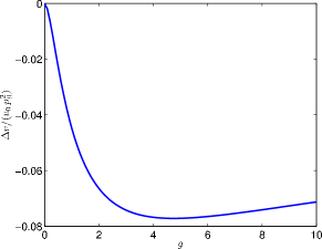
Figure 7: (Color online) Relative renormalization $\Delta v/(v_{0}p_{0}^{2})\equiv(v-v_{0})/(v_{0}p_{0}^{2})=-g_{5}/(2x_{0}^{2})$ of the ZS velocity in units of $p_{0}^{2}$ as a function of the interaction strength $g$, see Eq. (129).

Obviously, even for large $g$ and $p_{0}^{2}=O(1)$ the correction to the RPA result $v_{0}$ never exceeds more than a few percent.

V.3 Ad hoc regularization of the mass-shell singularity and spectral line-shape

Although for sharp momentum-transfer cutoff the dynamic structure factor exhibits (within approximation A discussed in Sec. IV.2) a mass-shell singularity at the ZS energy $v|q|$, it is nevertheless instructive to follow Samokhin Samokhin98 and regularize the singularity by hand using the procedure outlined in Sec. II. Because the natural scale for the momentum dependence is not $2k_{F}$ but the scale $q_{0}$ set by the momentum-transfer cutoff, it is convenient to express the momentum dependence via $\tilde{q}=q/q_{0}$. Setting $p=p_{0}\tilde{q}$ and writing

$$S(\omega,q)=\frac{\nu_{0}}{\pi}{\rm Im}\left[\frac{1}{g_{0}+\tilde{\Pi}_{\ast}^{-1}(x+i0,\tilde{q})}\right],$$ (130)

we obtain on the imaginary frequency axis

$$g_{0}+\tilde{\Pi}_{\ast}^{-1}(iy,\tilde{q}) = \Delta\left[1+p_{0}^{2}(g_{2}+g_{4}|\tilde{q}|)\right]-p_{0}^{2}g_{6}|\tilde{q}|$$ (131)

$$+ p_{0}^{2}\tilde{q}^{2}\Biggl{\{}h_{0}-\frac{h_{1}}{\Delta}+\Delta\biggl{[}g_{7}+g_{8}\ln\Bigl{(}1+\frac{4x_{0}^{2}(1-|\tilde{q}|)}{\tilde{q}^{2}\Delta}\Bigr{)}\biggr{]}$$

$$\hskip 28.45274pt+(g-\Delta)\frac{b^{2}}{a^{3}x_{0}}{\rm Re}\biggl{[}(1-iy)(x_{0}-iy)\ln\Bigl{(}\frac{a-|\tilde{q}|(x_{0}-iy)}{a+|\tilde{q}|(1+iy)}\Bigr{)}\biggr{]}\Biggr{\}},$$

where

$$g_{6} = x_{0}^{2}g_{4}-g_{3}=\frac{b^{2}}{ax_{0}^{3}}g\left[2+g-\frac{b}{g}\left(1+\frac{g}{4}\right)\right]=\frac{3}{16}g^{3}+O(g^{4}),$$ (132a)

$$g_{7} = \frac{1}{2}+\frac{3}{2x_{0}}-\frac{8}{g}\Bigl{(}\frac{a}{4}-\frac{b}{g}\Bigr{)}=\frac{1}{8}g^{2}-\frac{11}{64}g^{3}+O(g^{4}),$$ (132b)

$$g_{8} = \frac{g^{2}}{16x_{0}^{5}}=\frac{1}{16}g^{2}-\frac{5}{32}g^{3}+O(g^{4}),$$ (132c)

$$h_{0} = -1+\frac{2g}{3x_{0}}+\frac{b}{2gx_{0}}[8+4g-g^{2}]=1+\frac{1}{6}g-\frac{1}{12}g^{2}+O(g^{3}),$$ (132d)

$$h_{1} = \frac{(1+3x_{0}^{2})^{2}}{12x_{0}}=\frac{(4+3g)^{2}}{12x_{0}}=\frac{4}{3}+\frac{4}{3}g+\frac{1}{4}g^{2}+O(g^{3}).$$ (132e)

From Eq. (131) it is obvious that our functional bosonization approach yields a systematic expansion of the inverse irreducible polarization in powers of the small parameter $p_{0}=q_{0}/(2k_{F})$. Note that only $h_{0}$ and $h_{1}$ have finite limits for $g\rightarrow 0$, whereas the other couplings $g_{1},\ldots,g_{8}$ vanish at least as $g^{2}$ (the coupling $g_{6}$ vanishes even as $g^{3}$).

In the limit $g\rightarrow 0$ Eq. (131) correctly reduces to the expansion of the non-interacting inverse polarization given in Eq. (31). However, the term $h_{1}/\Delta$ generates a mass-shell singularity at the true collective mode energy $\omega=\pm vq$. Fortunately, this singularity can be avoided if we use a more physical interaction whose Fourier transform $f_{q}$ is analytic for small $q$, as will be shown explicitly in Sec. VI. In this subsection we shall simply regularize the mass-shell singularity by hand using the self-consistent regularization procedure proposed by Samokhin Samokhin98 , which we have already described in detail in Sec. II. Repeating the steps leading from Eq. (38) to Eq. (43), we obtain from the self-consistent regularization of the singular term proportional to $h_{1}/\Delta$ in Eq. (131) the following estimate for the width of the ZS mode,

$$\text{w}_{q}=\frac{\sqrt{h_{1}}}{2x_{0}}\frac{q^{2}}{2m}=Z_{\rm w}\frac{q^{2}}{2\sqrt{3}m},$$ (133)

where we have factored out the corresponding estimate in the absence of interactions given in Eq. (43), and the dimensionless factor $Z_{\rm w}$ is given by

$$Z_{\rm w}=\sqrt{\frac{3h_{1}}{4x_{0}^{2}}}=\frac{1+\frac{3}{4}g}{[1+g]^{3/4}}.$$ (134)

Note that $Z_{\rm w}\sim 1+\frac{3}{32}g^{2}+O(g^{3})$ for $g\rightarrow 0$, and $Z_{\rm w}\sim\frac{3}{4}g^{1/4}$ for $g\rightarrow\infty$. A graph of $Z_{\rm w}$ as a function of the interaction strength $g$ is shown in Fig. 8.

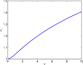
Figure 8: (Color online) Graph of the factor $Z_{\rm w}$ defined in Eq. (134), which estimates the interaction-induced relative change of the width of ZS resonance for $q\ll q_{c}$, see Eqs. (133,134).

The estimate (133) for the width of the ZS resonance on the frequency axis scales as $q^{2}$, which is for small $q$ much larger than our previous estimate (120) based on the evaluation of only the first-order diagram (a) in Fig. 2. The $q^{2}$-scaling of the width of the ZS resonance has already been found by Samokhin Samokhin98 and has been confirmed later in Refs.[Pustilnik03, ; Pustilnik06, ; Pereira06, ]. However, the derivation of Eq. (133) is based on a rather ad hoc regularization prescription of the mass-shell singularity in Eq. (131), which ignores in particular the divergent real part of the term $h_{1}/\Delta$. Let us nevertheless proceed and calculate the corresponding dynamic structure factor, which can be obtained by replacing the term $h_{1}/\Delta=h_{1}/(x_{0}^{2}+y^{2})$ on the right-hand side of Eq. (131) by

$$\frac{h_{1}}{\Delta}\rightarrow\frac{h_{1}}{x_{0}^{2}-\frac{(\omega+i\text{w}_{q})^{2}}{(v_{F}q)^{2}}}.$$ (135)

The finite imaginary part $\text{w}_{q}$ in this expression is a rough estimate of the modification of the spectral line-shape due to the terms which have been neglected by making the approximation A discussed in Sec. IV.2. The typical form of the dynamic structure factor in the regime $p\ll p_{0}$ implied by Eqs. (131, 133) and (135) is shown in Fig. 9.

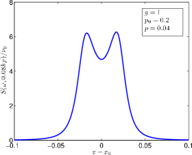
Figure 9: (Color online) Graph of the dynamic structure factor $S(\omega,q)$ as a function of $x-x_{0}=(\omega-vq)/(v_{F}q)$ for fixed $q=0.08k_{F}$. The line-shape has been calculated from Eqs. (131, 133) and (135). The distance between the local maxima is proportional to $\text{w}_{q}\propto q^{2}/m$.

Obviously, within our approximation the dynamic structure factor does not exhibit any threshold singularities, which according to Refs. [Pustilnik06, ; Pereira06, ] are a generic feature of the dynamic structure factor of Luttinger liquids. It turns out that the absence of threshold singularities in Fig. 9 is an artefact of the rather simple regularization prescription (135) of the unphysical mass-shell singularity in Eq. (131). In the following section we shall show how to recover the threshold singularities within our functional bosonization approach.

VI Interaction with regular momentum dependence

In this section we shall show that for a more realistic interaction whose Fourier transform is for small momenta of the form $f_{q}=f_{0}+\frac{1}{2}f_{0}^{\prime\prime}q^{2}+O(q^{4})$ with $f_{0}^{\prime\prime}\neq 0$ we do not encounter any mass-shell singularities. In fact, we believe that even for sharp momentum-transfer cutoff, $f_{q}=f_{0}\Theta(q_{0}-q)$, our perturbative result (67) does not suffer from mass-shell singularities as long as we do not rely on the approximation A discussed in Sec. IV.2; in other words, the mass-shell singularity $h_{1}/\Delta$ in Eq. (131) is an artefact of the sharp momentum-transfer cutoff in combination with our neglect of curvature corrections to the free polarization in loop integrations. While we are not able to evaluate Eqs. (80–83) analytically without relying on approximation A, we shall in this section abandon the sharp momentum-transfer cutoff and assume that the interaction $f_{q}$ can be expanded for small $q$ as in Eq. (15). Later we shall argue that as long as we rely on approximation A, our result for $S(\omega,q)$ can only be trusted for $q\gtrsim q_{c}=1/(m|f_{0}^{\prime\prime}|)$, see Eq. (16). But if $f_{0}^{\prime\prime}$ is sufficiently large, then there exists a parametrically large regime $q_{c}\ll q\ll k_{F}$ of wave-vectors where our calculation is valid.

VI.1 Imaginary part of $\Pi_{\ast}^{-1}(\omega,q)$

Let us first calculate the imaginary part of the dimensionless inverse polarization $\tilde{\Pi}^{-1}_{\ast}(x+i0,p)$ given in Eq. (110) assuming for simplicity $p>0$. From Eqs. (111) and (113) we obtain

$${\rm Im}\tilde{\Pi}^{-1}_{\ast}(x+i0,p) = {\rm Im}\tilde{I}(x+i0,p)$$

$$=\frac{1}{2}\int_{0}^{\infty}dp^{\prime}p^{\prime}{\rm Im}\left[\tilde{J}(x+i0,p,p^{\prime})+\tilde{J}(-x-i0,p,p^{\prime})\right].$$

In order to calculate the imaginary part of $\tilde{J}(x+i0,p,p^{\prime})$, we first perform a partial fraction decomposition of Eq. (113), then carry out the analytic continuation to the real frequency axis $iy\rightarrow x+i0$, and finally take the imaginary part using ${\rm Im}[a-x-i0]^{-1}=\pi\delta(a-x)$. After some lengthy algebra we obtain

$${\rm Im}\tilde{J}(x+i0,p,p^{\prime}) = -\frac{\pi|p^{\prime}+p|}{2x_{p^{\prime}}x_{p^{\prime}+p}}\Biggl{\{}\Theta(p^{\prime}+p)\Bigl{[}1-x_{p^{\prime}}x_{p^{\prime}+p}-x(x_{p^{\prime}}-x_{p^{\prime}+p})\Bigr{]}^{2}\delta\Bigl{(}p^{\prime}(x_{p^{\prime}}+x_{p^{\prime}+p})-p(x-x_{p^{\prime}+p})\Bigr{)}$$

$$+\Theta(-p^{\prime}-p)\Bigl{[}1+x_{p^{\prime}}x_{p^{\prime}+p}-x(x_{p^{\prime}}+x_{p^{\prime}+p})\Bigr{]}^{2}\delta\Bigl{(}p^{\prime}(x_{p^{\prime}}-x_{p^{\prime}+p})-p(x+x_{p^{\prime}+p})\Bigr{)}\Biggr{\}}-(p\rightarrow-p)$$

$$= -\frac{\pi|p^{\prime}+p|}{2x_{p^{\prime}}x_{p^{\prime}+p}}\Bigl{[}1-x_{p^{\prime}}\tilde{x}_{p^{\prime}+p}-x(x_{p^{\prime}}-\tilde{x}_{p^{\prime}+p})\Bigr{]}^{2}\delta\Bigl{(}p^{\prime}(x_{p^{\prime}}+\tilde{x}_{p^{\prime}+p})-p(x-\tilde{x}_{p^{\prime}+p})\Bigr{)}-(p\rightarrow-p),$$

where we have defined $\tilde{x}_{p+p^{\prime}}={\rm sign}(p+p^{\prime}){x}_{p+p^{\prime}}$. In order to perform the $p^{\prime}$-integration in Eq. (LABEL:eq:ImPi), we use the fact that by assumption both $p$ and $p^{\prime}$ are small compared with unity so that we may expand $x_{p}$ to first order in $p^{2}$,

$$x_{p} = \sqrt{1+\tilde{g}_{p}}$$ (138)

$$= \sqrt{1+g+\frac{g_{0}^{\prime\prime}}{2}p^{2}+O(p^{4})}$$

$$= x_{0}+\frac{x_{0}^{\prime\prime}}{2}p^{2}+O(p^{4}),$$

where from Eq. (77),

$$x_{0}^{\prime\prime}=\frac{{\rm sign}f_{0}^{\prime\prime}}{\pi x_{0}p_{c}}.$$ (139)

Note that for small $p_{c}$ the coefficient $x_{0}^{\prime\prime}$ is large compared with unity. The $\delta$-functions in Eq. (LABEL:eq:ImJ) can then be approximated by

$$\delta\Bigl{(}p^{\prime}(x_{p^{\prime}}+x_{p^{\prime}+p})-p(x-x_{p^{\prime}+p})\Bigr{)}$$ (140)

$$\approx\frac{1}{2x_{p}}\delta\Bigl{(}p^{\prime}-p\frac{x-x_{p}}{2x_{p}}\Bigr{)},$$

$$\delta\Bigl{(}p^{\prime}(x_{p^{\prime}}-x_{p^{\prime}+p})-p(x+x_{p^{\prime}+p})\Bigr{)}$$ (141)

$$\approx\frac{2}{3|x_{0}^{\prime\prime}p|}\delta\Bigl{(}p^{\prime 2}+p^{\prime}p+\frac{2(x+x_{p})}{3x_{0}^{\prime\prime}}\Bigr{)}.$$

In Eq. (140) we have expanded the argument of the $\delta$-function to linear order in $p$ and $p^{\prime}$, assuming that both dimensionless momenta are small. On the other hand, due to the cancellation of the leading term in the difference $x_{p^{\prime}}-x_{p^{\prime}+p}$ in the $\delta$-function of Eq. (141), the corresponding expansion has to be carried out to cubic order in the momenta. The integration in Eq. (LABEL:eq:ImJ) can now be carried out analytically and we obtain for small $p>0$,

$${\rm Im}\tilde{\Pi}^{-1}_{\ast}(x+i0,p) = -\pi^{2}p_{c}\Biggl{[}\Theta(x-x_{p})\tilde{g}_{p}^{2}\tilde{\gamma}_{p}\frac{x^{2}-x_{p}^{2}}{12x_{0}^{4}}$$ (142)

$$\hskip 28.45274pt+h_{1}C_{I}\Bigl{(}\frac{x-x_{p}}{\tilde{\gamma}_{p}}\Bigr{)}\Biggr{]},$$

where

$$\tilde{\gamma}_{p}=\frac{3p^{2}}{8\pi x_{0}p_{c}},$$ (143)

and the function $C_{I}(u)$ is given by

$$C_{I}(u)=\Theta(u)\Theta(1-u)\frac{u}{\sqrt{1-u}}.$$ (144)

Note that the coefficient $h_{1}=(1+3x_{0}^{2})^{2}/(12x_{0})$ on the right-hand side of Eq. (142) has also appeared for sharp momentum-transfer cutoff [see Eq. (132e)] in form of the residue of the mass-shell singularity $h_{1}/\Delta$ in our expression (131) for the irreducible polarization. A graph of $C_{I}(u)$ is shown as the dashed line in Fig. 10.

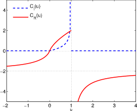
Figure 10: (Color online) Graph of the functions $C_{I}(u)$ and $C_{R}(u)$ defined in Eqs. (144) and (148). The dotted lines indicate asymptotic limits.

Mathematically, the square-root singularity of $C_{I}(u)$ for $u\rightarrow 1$ originates from the special point $x-x_{p}=\tilde{\gamma}_{p}$ where the argument of the Dirac $\delta$-function on the right-hand side of Eq. (140) has a double root. We believe that the divergence of $C_{I}(u)$ for $u\rightarrow 1$ is unphysical and indicates that the approximations leading to Eq. (140) are not sufficient in this regime. Hence, within our approximations we can only obtain reliable results for the spectral line-shape as long as the ratio $(x-x_{p})/\tilde{\gamma}_{p}$ is not too close to unity.

VI.2 Real part of $\Pi_{\ast}^{-1}(\omega,q)$

For $p_{c}\ll 1$ and $p\ll 1$ we can obtain the contribution from ${\rm Re}\tilde{I}(x+i0,p)$ analytically from Eqs. (111) and (113) using the fact that among the corrections of order $p^{2}$ only terms proportional to $p^{2}/p_{c}$ should be retained. We obtain for $x>0$ and $p>0$,

$${\rm Re}\tilde{I}(x+i0,p) = I_{1}-x^{2}I_{2}$$ (145)

$$+ \pi p_{c}h_{1}{\rm sign}f_{0}^{\prime\prime}C_{R}\Bigl{(}\frac{x-x_{p}}{\tilde{\gamma}_{p}}\Bigr{)},\hskip 28.45274pt$$

where

$$I_{1} = -\int_{0}^{\infty}dpp\frac{(x_{p}-1)^{2}}{2x_{p}^{3}}(3x_{p}^{2}+2x_{p}+1)$$ (146)

$$+2\pi p_{c}h_{1}{\rm{sign}}f_{0}^{\prime\prime},$$

$$I_{2} = \int_{0}^{\infty}dpp\frac{(x_{p}-1)^{2}}{x_{p}},$$ (147)

and the function $C_{R}(u)$ is given by

$$C_{R}(u) = \frac{u}{\sqrt{|1-u|}}\Biggl{[}\Theta(1-u)\ln\left|\frac{1+\sqrt{1-u}}{1-\sqrt{1-u}}\right|$$ (148)

$$-2\Theta(u-1)\arctan\left(\frac{1}{\sqrt{u-1}}\right)\Biggr{]}.$$

A graph of $C_{R}(u)$ is shown in Fig. 10 (solid line). Note that $C_{R}(u)$ and $C_{I}(u)$ can be written as $C_{R}(u)={\rm Re}C(u+i0)$ and $C_{I}(u)={\rm Im}C(u+i0)$, where the complex function $C(z)$ is

$$C(z)=\frac{z}{i\sqrt{1-z}}\ln\left(\frac{\sqrt{1-z}+1}{\sqrt{1-z}-1}\right).$$ (149)

The real part of our dimensionless inverse polarization can be written as

$${\rm Re}\tilde{\Pi}^{-1}_{\ast}(x+i0,p) = Z_{1}-Z_{2}x^{2}$$ (150)

$$+ \pi p_{c}h_{1}{\rm{sign}}f_{0}^{\prime\prime}C_{R}\Bigl{(}\frac{x-x_{p}}{\tilde{\gamma}_{p}}\Bigr{)},\hskip 28.45274pt$$

with

$$Z_{1}=1+I_{1}+I_{H},\;\;\;Z_{2}=1+I_{2}-I_{H}.$$ (151)

By assumption, the bare interaction $f_{q}$ is negligibly small for momentum-transfers exceeding $q_{0}\ll k_{F}$, so that the integrals $I_{1}$, $I_{2}$ and $I_{H}$ are proportional to $p_{0}^{2}=[q_{0}/(2k_{F})]^{2}\ll 1$ and hence $Z_{i}=1+O(p_{0}^{2})$. Keeping in mind the self-consistent definition (74) of $x_{0}$, we finally obtain for positive $x$ and $p$,

$$g_{p}+{\rm Re}\tilde{\Pi}^{-1}_{\ast}(x+i0,p)=Z_{2}\Bigl{[}x_{p}^{2}-x^{2}+R(x,p)\Bigr{]},$$ (152)

where

$$R(x,p)=\frac{\pi p_{c}h_{1}}{Z_{2}}{\rm{sign}}f_{0}^{\prime\prime}C_{R}\Bigl{(}\frac{x-x_{p}}{\tilde{\gamma}_{p}}\Bigr{)}.$$ (153)

VI.3 Spectral line-shape of $S(\omega,q)$

To discuss the line-shape of the dynamic structure factor, it is convenient to introduce also the imaginary part of the effective self-energy via

$${\rm Im}\tilde{\Pi}^{-1}_{\ast}(x+i0,p)=-Z_{2}\Gamma(x,p),$$ (154)

or explicitly,

$$\Gamma(x,p) = \frac{\pi^{2}p_{c}}{Z_{2}}\Bigl{[}\Theta(x-x_{p})\tilde{g}_{p}^{2}\tilde{\gamma}_{p}\frac{x^{2}-x_{p}^{2}}{12x_{0}^{4}}$$ (155)

$$\hskip 28.45274pt+h_{1}C_{I}\Bigl{(}\frac{x-x_{p}}{\tilde{\gamma}_{p}}\Bigr{)}\Bigr{]}.$$

The dynamic structure factor can then we written as

$$S(\omega,q)=\frac{\nu_{0}}{\pi Z_{2}}\frac{\Gamma(x,p)}{[x^{2}-x_{p}^{2}-R(x,p)]^{2}+\Gamma^{2}(x,p)}.$$ (156)

The resulting line-shape for $p\gg p_{c}$ is shown in Fig. 11.

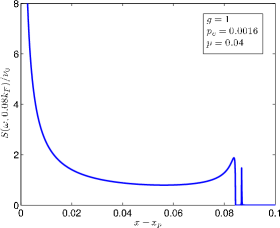
Figure 11: (Color online) Graph of the dynamic structure factor $S(\omega,q)$ given in Eq. (156) as a function of $x-x_{p}$ for $p=0.04=25p_{c}$ and ${g}=1$. For simplicity we have set $Z_{2}\approx 1$, which is accurate for $p_{0}\ll 1$. For $p\gg p_{c}$ most of the spectral weight is carried by the main shoulder whose lower edge $x\rightarrow x_{p}$ is bounded by a threshold singularity. The width of the main shoulder on the $x$ axis scales as $\tilde{\gamma}_{p}\propto p^{2}/p_{c}$. Recall that $x=\omega/(v_{F}q)$, so that the corresponding width on the frequency axis scales as $\gamma_{q}=v_{F}q\tilde{\gamma}_{p}\propto q^{3}/(mq_{c})$. For $p\gg p_{c}$ the small “satellite peak” emerging above the upper edge of the main shoulder carries negligible spectral weight and is probably an artefact of our approximations.

Obviously, $S(\omega,q)$ exhibits a threshold singularity at $x=x_{p}$, corresponding to the threshold frequency

$$\omega_{q}^{-}\equiv v_{F}qx_{p}=vq+\frac{{\rm sign}f_{0}^{\prime\prime}}{2\pi x_{0}}\frac{q^{3}}{2mq_{c}}.$$ (157)

Moreover, most of the spectral weight is smeared out over the interval $0<x-x_{p}<\tilde{\gamma}_{p}$, or equivalently $\omega_{q}^{-}<\omega<\omega_{q}^{-}+\gamma_{q}$, where the energy scale $\gamma_{q}$ is defined by

$$\gamma_{q}=v_{F}q\tilde{\gamma}_{p}=\frac{3}{8\pi x_{0}}\frac{q^{3}}{2mq_{c}}.$$ (158)

The energy $\gamma_{q}$ can be identified with the width of the ZS resonance on the frequency axis. The crucial point is now that for $q\gg q_{c}$ Eq. (158) is much larger than the estimated broadening $\text{w}_{q}\propto q^{2}/m$ of the ZS resonance due to the terms which we have neglected by making the approximation A discussed in Sec. IV.2 (which amounts to ignoring non-linear terms in the energy dispersion in bosonic loop integrations). Our approximation A is therefore only justified in the regime where the broadening $\gamma_{q}$ due to the $q$-dependence of the interaction $f_{q}$ is large compared with the broadening $\text{w}_{q}$ due to the non-linear energy dispersion in bosonic loop integrations. We thus conclude that the calculations in this section are only valid as long as $\gamma_{q}\gtrsim\text{w}_{q}$. A comparison of $\gamma_{q}$ and $\text{w}_{q}$ is shown in Fig. 12.

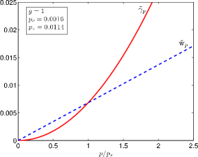
Figure 12: (Color online) Solid line: dimensionless ZS damping $\tilde{\gamma}_{p}=\gamma_{q}/(v_{F}q)$ defined in Eq. (158) as a function of $p/p_{\ast}$. Dashed line: estimate of the width $\tilde{\text{w}}_{p}=\text{w}_{q}/(v_{F}q)=(Z_{\rm w}/\sqrt{3})p$ of the ZS resonance given in Eq. (133).

Obviously, the condition $\text{w}_{q}=\gamma_{q}$ defines a characteristic crossover scale $q_{\ast}$ where the $q$-dependence of the width of the ZS resonance changes from $q^{2}$ to $q^{3}$. Using Eqs. (133) and (158) we obtain the following estimate for the crossover momentum scale,

$$q_{\ast}=\frac{8\pi Z_{\rm w}x_{0}}{3\sqrt{3}}q_{c},$$ (159)

which has the same order of magnitude as $q_{c}=1/(m|f_{0}^{\prime\prime}|)$. We conclude that the results for $S(\omega,q)$ presented in this section are only valid for $q\gtrsim q_{\ast}$, and hence do not describe the asymptotic $q\rightarrow 0$ regime. But the scale $q_{\ast}$ can be quite small for some interactions. For example, if the interaction $f_{q}$ can be approximated by a Lorentzian (13) with screening wave-vector $q_{0}\ll k_{F}$, then $q_{c}=q_{0}^{2}/(2mf_{0})$ is quadratic in $q_{0}$. For long-range interactions the regime $q_{\ast}\lesssim q\ll q_{0}$ where our calculation is valid can therefore be quite large and physically more relevant than the asymptotic long-wavelength regime $q\ll q_{\ast}$.

The small “satellite peak” slightly above the main shoulder in Fig. 11 is probably an artefact of our approximations, in particular of approximation A discussed in Sec. IV.2. It is easy to show that the satellite peak is located a distance $\delta x\propto p_{c}^{3}/p^{2}\ll\tilde{\gamma}_{p}$ above the upper edge $x_{p}+\tilde{\gamma}_{p}$ of the main shoulder and its width is proportional to $p^{2}\tilde{\gamma}_{p}\propto p^{4}/p_{c}\ll\delta x\ll\tilde{\gamma}_{p}$. Note that in the regime $q\gg q_{c}$ where our calculation is valid the threshold singularity is located at $\omega_{q}^{-}\approx vq-\gamma_{q}$ (up to corrections of the order $q^{2}/m\ll\gamma_{q}$), while the energy scale of the satellite peak is $vq+O(q^{2}/m)$. However, as discussed after Eq. (144), in the regime $|(x-x_{p})/\tilde{\gamma}_{p}-1|\ll 1$ our approximation A is not reliable, so that the detailed line-shape in the vicinity of the satellite peak is probably incorrect. Fortunately, for $p\gg p_{c}$ the satellite peak carries negligible weight, so that our calculation reproduces the main features of the spectral line-shape. We speculate that a more accurate evaluation of our self-consistency equation for $\Pi_{\ast}(\omega,q)$ derived in Sec. IV.1, which does not rely on approximation A in Sec. IV.2, will generate additional weight in the dip between the upper edge of the main shoulder and the satellite peak, resulting in a single local maximum at the upper edge of the main shoulder. The spectral line-shape looks then qualitatively similar to the line-shape proposed in Refs. [Pustilnik06, ; Pereira06, ].

Let us next consider the line-shape in the vicinity of the threshold singularity $x\rightarrow x_{p}$. For $0<(x-x_{p})/\tilde{\gamma}_{p}\ll 1$ we may approximate

$$\Gamma(x,p) \approx \frac{\pi^{2}p_{c}h_{1}}{Z_{2}}\frac{x-x_{p}}{\tilde{\gamma}_{p}}$$ (160)

$$= 2\pi x_{0}|\eta_{p}|(x-x_{p}),$$

$$R(x,p) \approx \frac{\pi p_{c}h_{1}}{Z_{2}}\frac{x-x_{p}}{\tilde{\gamma}_{p}}\ln\left[\frac{4\tilde{\gamma}_{p}}{x-x_{p}}\right]$$ (161)

$$= -2x_{0}\eta_{p}(x-x_{p})\ln\left[\frac{4\tilde{\gamma}_{p}}{x-x_{p}}\right],$$

where we have defined

$$\eta_{p} = -{\rm sign}f_{0}^{\prime\prime}\frac{\pi p_{c}h_{1}}{2Z_{2}x_{0}\tilde{\gamma}_{p}}$$ (162)

$$= -{\rm sign}f_{0}^{\prime\prime}\frac{4\pi^{2}h_{1}}{3Z_{2}}\frac{p_{c}^{2}}{p^{2}}$$

$$= -{\rm sign}f_{0}^{\prime\prime}\frac{3p_{\ast}^{2}}{4p^{2}}.$$

In the last line we have approximated $Z_{2}\approx 1$. From the above discussion it is clear that this expression can only be trusted for $p\gtrsim p_{\ast}$. A graph of $\eta_{p}$ as a function of $p/p_{\ast}$ is shown in Fig. 13.

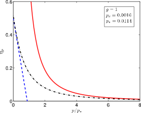
Figure 13: (Color online) Solid line: graph of $\eta_{p}$ defined in Eq. (162) as a function of $p/p_{\ast}$ for $f_{0}^{\prime\prime}<0$. The dashed line is the weak coupling result $\eta_{p}\approx 1/2-p/(4\pi p_{c})$ obtained by Pustilnik et al. in Ref. [Pustilnik06, ]. The dashed dotted curve is a simple parabolic interpolation.

In the regime $|\eta_{p}|\ln[4\tilde{\gamma}_{p}/(x-x_{p})]\gg 1$, which is equivalent with

$$0<x-x_{p}\ll 4\tilde{\gamma}_{p}\exp\left[-1/|\eta_{p}|\right],$$ (163)

the dynamic structure factor can thus be approximated by

$$S(\omega,q)\sim\frac{\nu_{0}}{2x_{0}Z_{2}|\eta_{p}|}\frac{1}{(x-x_{p})\ln^{2}\left[\frac{4\tilde{\gamma}_{p}}{x-x_{p}}\right]}.$$ (164)

According to Pustilnik et al. Pustilnik06 , the logarithmic singularity can be re-summed to all orders, so that it is transformed into an algebraic one. Assuming that this is indeed correct, we can replace

$$x^{2}-x_{p}^{2}-R(x,p) \approx 2x_{0}(x-x_{p})\left\{1+\eta_{p}\ln\left[\frac{4\tilde{\gamma}_{p}}{x-x_{p}}\right]\right\}$$ (165)

$$\rightarrow 2x_{0}(x-x_{p})\left[\frac{4\tilde{\gamma}_{p}}{x-x_{p}}\right]^{\eta_{p}}.$$

For $x\rightarrow x_{p}$ the dynamic structure factor then diverges as

$$S(\omega,q)\sim\frac{\nu_{0}}{2x_{0}Z_{2}}\frac{|\eta_{p}|}{(4\tilde{\gamma}_{p})^{2\eta_{p}}}\frac{1}{[x-x_{p}]^{\mu_{p}}},$$ (166)

with the threshold exponent

$$\mu_{p}=1-2\eta_{p}=1+{\rm sign}f_{0}^{\prime\prime}\frac{3p_{\ast}^{2}}{2p^{2}}.$$ (167)

Note that for $f_{0}^{\prime\prime}<0$ and $p\ll 1$ the weak coupling estimate for $\mu_{p}$ given by Pustilnik et al.Pustilnik06 is in our notation

$$\mu_{p}\approx\frac{p}{2\pi p_{c}},$$ (168)

implying

$$\eta_{p}=\frac{1}{2}[1-\mu_{p}]=\frac{1}{2}\left[1-\frac{p}{2\pi p_{c}}\right].$$ (169)

As shown in Fig. 13, this is consistent with a smooth crossover to our result (162) at $p/p_{\ast}=O(1)$. Qualitatively, we expect that the behavior of $\eta_{p}$ in the crossover regime resembles the dashed-dotted interpolation curve in Fig. 13. Note that $\eta_{p}\leq 1/2$ for all $p$, so that $\mu_{p}\geq 0$. For some integrable models where $\eta_{p}$ has recently been calculated exactly Pustilnik06b ; Cheianov07 the momentum-dependence of $\eta_{p}$ looks different from our result for the FSM. For example, in the Calogero-Sutherland model $\eta_{p}$ is independent of $p$, see Ref. [Pustilnik06b, ]. However, the Fourier transform $f_{q}$ of the interaction in the Calogero-Sutherland model vanishes for $q=0$, while in the integrable XXZ-chain considered in Refs. [Pereira06, ; Pereira07, ; Pereira07b, ; Cheianov07, ] the effective interaction of the equivalent one-dimensional fermion system involves also momentum-transfers of the order of $k_{F}$. Moreover, in the XXZ-chain there exists no crossover scale $q_{c}$ satisfying $q_{c}=(m|f_{0}^{\prime\prime}|)^{-1}\ll k_{F}$, so that the intermediate regime $q_{c}\ll q\ll k_{F}$ where $\gamma_{q}\propto q^{3}/q_{c}$ simply does not exist. The existence of such an intermediate regime seems to be a special feature of the FSM considered here, where $f_{q}$ involves only small momentum-transfers and has a finite limit for $q=0$.

Within our perturbative approach we cannot justify the re-summation procedure (165). Possibly a careful analysis of the functional renormalization group flow equation for the irreducible polarization discussed in appendix D will shed some light onto this difficult problem. This seems to require extensive numerics, which is beyond the scope of this work. Note that for $f_{0}^{\prime\prime}>0$ the exponent $\eta_{p}$ in Eq. (162) is negative, so that the singularity in Eq. (166) is not integrable and exact sum rules Pines89 cannot be satisfied. In contrast, the original logarithmic singularity in Eq. (164) is integrable (the integral $\int_{0}dt/[t\ln^{2}t]$ is finite), so that at least for $f_{0}^{\prime\prime}>0$ the logarithm found in perturbation theory cannot be exponentiated. On the other hand, an interaction with $f_{0}^{\prime\prime}>0$ seems to be unphysical and does not describe a stable Luttinger liquid footnoteessler .

Finally, consider the tails of the spectral function. For $x\gg x_{p}$ we obtain from Eqs. (155) and (156),

$$S(\omega,q)\sim\frac{\nu_{0}}{\pi Z_{2}}\frac{\Gamma(x,p)}{x^{4}},$$ (170)

$$\Gamma(x,p)\sim\frac{\pi^{2}p_{c}}{12Z_{2}x_{0}^{4}}\tilde{g}_{p}^{2}\tilde{\gamma}_{p}x^{2}.$$ (171)

Inserting our result (143) for $\tilde{\gamma}_{p}$ we obtain

$$S(\omega,q)\sim\frac{\nu_{0}\tilde{g}_{p}^{2}}{32Z_{2}^{2}x_{0}^{5}}\left[\frac{q^{2}}{2m\omega}\right]^{2},$$ (172)

in agreement with Refs. [Teber06, ; Pereira06, ; Pereira07, ; Aristov07, ]. Note that the tail of $S(\omega,q)$ is determined by the first term on the right-hand side of the damping function $\Gamma(x,p)$ given in Eq. (155), whereas the regime close to the ZS resonance is determined by the second term involving the complex function $C(z)$. This is the reason why the spectral line-shape close to the ZS resonance cannot be simply obtained via extrapolation from the tails assuming a Lorentzian line-shape.

VII Summary and Conclusions

In this work we have used a functional bosonization approach to calculate the dynamic structure factor $S(\omega,q)$ of a generalized Tomonaga model (which we have called forward scattering model), consisting of spinless fermions in one dimension with quadratic energy dispersion and an effective density-density interaction involving only momentum-transfers which are small compared with $k_{F}$. We have derived in Sec. IV a self-consistency equation for the irreducible polarization $\Pi_{\ast}(\omega,q)$ which does not suffer from the mass-shell singularities encountered in other perturbative approaches. Although for the explicit evaluation of $S(\omega,q)$ we had to make some drastic approximations (in particular, in bosonic loop integrations we have neglected curvature corrections to the free polarization, see approximation A discussed in Sec. IV.2) we have found a regime of wave-vectors $q_{c}\ll q\ll k_{F}$ where an explicit analytic calculation of the spectral line-shape is possible. The crossover scale $q_{c}=1/(m|f_{0}^{\prime\prime}|)$ is determined by the second derivative $f_{0}^{\prime\prime}$ of the Fourier transform of interaction at $q=0$. For interactions whose Fourier transform can be approximated by a Lorentzian with screening wave-vector $q_{0}\ll k_{F}$, the crossover scale $q_{c}$ is proportional to $q_{0}^{2}$, so that the regime $q_{c}\ll q\ll k_{F}$ is quite large and can be experimentally more relevant than the asymptotic long-wavelength regime $q\ll q_{c}$. We have shown that for $q_{c}\ll q\ll k_{F}$ the width of the ZS resonance on the frequency axis scales as $\gamma_{q}\propto q^{3}/(mq_{c})$. Our result is consistent with a smooth crossover at $q\approx q_{c}$ to the asymptotic long-wavelength result $\gamma_{q}\propto q^{2}/m$ obtained by other authors Samokhin98 ; Pustilnik06 ; Pereira06 . The spectral line-shape is non-Lorentzian, with a main hump whose low-energy side is bounded by a threshold singularity at $\omega=\omega_{q}^{-}=vq-\gamma_{q}$, a small local maximum around $\omega\approx vq$, and a high-frequency tail which scales as $q^{4}/\omega^{2}$. For $\omega\rightarrow\omega_{q}^{-}+0$ the threshold singularity is within our approximation logarithmic, $S(\omega,q)\propto[(\omega-\omega_{q}^{-})\ln^{2}(\omega-\omega_{q}^{-})]^{-1}$. Assuming that higher orders in perturbation theory exponentiate the logarithm, we obtain an algebraic threshold singularity with exponent $\mu_{q}=1-2\eta_{q}$ and $\eta_{q}\propto q_{c}^{2}/q^{2}$ for $q\gg q_{c}$.

Finally, let us point out a number of open problems:

1. It is by now established that, at least in integrable models, $S(\omega,q)$ indeed exhibits algebraic threshold singularities Pustilnik06b ; Cheianov07 ; Pereira06 ; Pereira07 ; Pereira07b . However, for generic non-integrable models there is no proof that the logarithmic singularities generated in higher orders of perturbation theory indeed conspire to transform the logarithm encountered at the first order into an algebraic singularity, as suggested in Ref. [Pustilnik06, ]. This would require a thorough analysis of the higher order terms in perturbative expansion, which so far has not been performed.

2. For the explicit evaluation of the self-consistency equation for the irreducible polarization $\Pi_{\ast}(\omega,q)$ derived in Sec. IV.1 we had to rely in this work on approximation A discussed in Sec. IV.2. We have argued that this approximation is not sufficient to calculate the dynamic structure factor for $q\lesssim q_{c}$, because it neglects the dominant damping mechanism in this regime. Moreover, for sharp momentum-transfer cutoff our approximation A breaks down for frequencies in the vicinity of the mass-shell singularity. It would be interesting to evaluate the self-consistency equation for the irreducible polarization $\Pi_{\ast}(\omega,q)$ derived in Sec. IV.1 without relying on approximation A. We believe that in this case our functional bosonization result for $S(\omega,q)$ does not exhibit any mass-shell singularities even for sharp cutoff. The explicit evaluation of the relevant integrals is quite challenging and probably requires considerable numerical effort (including a numerical analytic continuation), which is beyond the scope of this work.

3. By assumption, the interaction of the FSM considered in this work is dominated by small momentum-transfers $q\ll k_{F}$. On the other hand, the Fourier transform of the effective interaction in the Jordan-Wigner transformed XXZ-chain studied in Refs. [Pereira06, ; Pereira07, ; Pereira07b, ] has also components involving momentum-transfers of the order of $k_{F}$. It should be interesting to investigate more thoroughly how the dynamic structure factor depends on the properties of the interaction. Unfortunately, the FSM discussed in this work is not integrable and there seems to be no integrable model with quadratic energy dispersion where the interaction involves only small momentum-transfers and has a finite limit for $q\rightarrow 0$.

4. In appendix D we present a functional renormalization group equation [see Eq. (225)] for the irreducible polarization which goes beyond the self-consistent perturbation theory based on functional bosonization used here. A thorough analysis of Eq. (225) using numerical methods still remains to be done. Possibly, this equation will be a good starting point for addressing some of the open problems mentioned above.

Appendix A Fermion loops for quadratic dispersion in one dimension

In the functional bosonization approach the vertices of the interaction part $S_{\rm int}[\delta\phi]$ of the bosonized action (63) are

$$\Gamma^{(n)}_{0}(Q_{1},\ldots,Q_{n})=i^{n}(n-1)!\;L^{(n)}_{S}(-Q_{1},\ldots,-Q_{n}),$$ (173)

where the symmetrized closed fermion loops are defined by

$$L^{(n)}_{S}(Q_{1},\ldots,Q_{n})$$ (174)

$$=\frac{1}{n!}\sum_{P(1,\ldots,n)}\int_{K}G_{0}(K)G_{0}(K-Q_{P(1)})$$

$$\times G_{0}(K-Q_{P(1)}-Q_{P(2)})\cdots G_{0}(K-\sum_{j=1}^{n-1}Q_{P(j)})\;.$$

Here the sum is over all permutations $P(1,\ldots,n)$ of $1,\ldots,n$, and the fermionic Green functions $G_{0}(K)$ should be calculated within the self-consistent Hartree approximation, see Eq. (59). For fermions with quadratic energy dispersion in one dimension, the symmetrized fermion loops (174) can be calculated exactly. Neumayr and Metzner Neumayr98 ; Neumayr99 (see also Ref. [Kopper01, ]) have derived reduction formulas for quadratic dispersion in $D$ dimensions which allow to express the non-symmetrized loops

$$\bar{L}^{(n)}(\bar{Q}_{1},\ldots,\bar{Q}_{n}) = \int_{K}\prod_{i=1}^{n}G_{0}(K-\bar{Q}_{i})$$ (175)

$$=\int_{K}G_{0}(K-\bar{Q}_{1})G_{0}(K-\bar{Q}_{2})\cdots G_{0}(K-\bar{Q}_{n}),$$

for $n>D+1$ in terms of linear combinations of the more elementary loop $\bar{L}^{(D+1)}(\bar{Q}_{1},\ldots,\bar{Q}_{D+1})$. In particular, in $D=1$ the non-symmetrized loops $\bar{L}^{(n)}(\bar{Q}_{1},\ldots,\bar{Q}_{n})$ with $n>2$ can be expressed in terms of the two-loop $\bar{L}^{(2)}(0,-{Q})=L^{(2)}_{S}(-Q,Q)=-\Pi_{0}(Q)$. Given explicit expressions for the non-symmetrized loops $\bar{L}^{(n)}(\bar{Q}_{1},\ldots,\bar{Q}_{n})$ we may construct the corresponding symmetrized loops $L^{(n)}_{S}(Q_{1},\ldots,Q_{n})$ by shifting the labels,

$$\bar{Q}_{1} = 0\;,$$

$$\bar{Q}_{2} = Q_{1}\;,$$

$$\bar{Q}_{3} = Q_{1}+Q_{2}\;,$$

$$\ldots$$

$$\bar{Q}_{n} = \sum_{j=1}^{n-1}Q_{j}\;,$$ (176)

so that $\bar{Q}_{i+1}-\bar{Q}_{i}=Q_{i}$, and defining

$${L}^{(n)}(Q_{1},\ldots,Q_{n})=\bar{L}^{(n)}(\bar{Q}_{1},\ldots,\bar{Q}_{n}).$$ (177)

Then the symmetrized loops are

$$L^{(n)}_{S}(Q_{1},\ldots,Q_{n})=\frac{1}{n!}\sum_{P(1,\ldots,n)}{L}^{(n)}(Q_{P(1)},\ldots,Q_{P(n)}).$$ (178)

In one dimension, the reduction formula for the non-symmetrized loop $\bar{L}^{(n)}(\bar{Q}_{1},\ldots,\bar{Q}_{n})$ given by Neumayr and Metzner Neumayr99 can be obtained using a straight-forward partial fraction decomposition. Performing the frequency integration in Eq. (175) and introducing the notation $\bar{Q}_{i}=(i\bar{\omega}_{i},\bar{q}_{i})$ we obtain

$$\bar{L}^{(n)}(\bar{Q}_{1},\ldots,\bar{Q}_{n})=\sum_{i=1}^{n}\int_{-k_{F}}^{k_{F}}\frac{dk}{2\pi}\prod_{\stackrel{{\scriptstyle j=1}}{{j\neq i}}}^{n}\frac{1}{\Omega_{ij}(k)},$$ (179)

where

$$\Omega_{ij}(k)=i(\bar{\omega}_{i}-\bar{\omega}_{j})+\xi_{k}-\xi_{k+\bar{q}_{i}-\bar{q}_{j}},$$ (180)

and $\xi_{k}=\frac{k^{2}}{2m}+f_{0}\rho_{0}-\mu=(k^{2}-k_{F}^{2})/(2m)$. Defining

$$k_{ij}=\frac{\bar{q}_{j}-\bar{q}_{i}}{2}+im\frac{\bar{\omega}_{j}-\bar{\omega}_{i}}{\bar{q}_{j}-\bar{q}_{i}},$$ (181)

we may alternatively write Eq. (179) as

$$\bar{L}^{(n)}(\bar{Q}_{1},\ldots,\bar{Q}_{n})=\sum_{i=1}^{n}\int_{-k_{F}}^{k_{F}}\frac{dk}{2\pi}\prod_{\stackrel{{\scriptstyle j=1}}{{j\neq i}}}^{n}\frac{m}{(\bar{q}_{j}-\bar{q}_{i})(k-k_{ij})}\,.$$ (182)

We can now perform another partial fraction expansion to obtain

$$\bar{L}^{(n)}(\bar{Q}_{1},\ldots,\bar{Q}_{n}) = \sum_{\stackrel{{\scriptstyle i,j=1}}{{i\neq j}}}^{n}\left[\prod_{\stackrel{{\scriptstyle l=1}}{{l\neq i,j}}}^{n}H_{ijl}\right]^{-1}\frac{m}{\bar{q}_{j}-\bar{q}_{i}}$$ (183)

$$\times\int_{-k_{F}}^{k_{F}}\frac{dk}{2\pi}\frac{1}{k-k_{ij}},$$

with

$$H_{ijl}=-\frac{(\bar{q}_{l}-\bar{q}_{i})(\bar{q}_{l}-\bar{q}_{j})}{2m}+i(\bar{\omega}_{i}-\bar{\omega}_{l})+i(\bar{\omega}_{j}-\bar{\omega}_{i})\frac{\bar{q}_{l}-\bar{q}_{i}}{\bar{q}_{j}-\bar{q}_{i}}.$$ (184)

In the special case $n=2$ this yields

$$\bar{L}^{(2)}(\bar{Q}_{1},\bar{Q}_{2})=\frac{m}{\pi(\bar{q}_{1}-\bar{q}_{2})}\ln\left|\frac{k_{F}+k_{12}}{k_{F}-k_{12}}\right|.$$ (185)

In order to give an explicit formula for the function $L^{(n)}(Q_{1},\ldots,Q_{n})$ defined in Eq. (177), which depends on the external momenta and frequencies $Q_{i}=(i\omega_{i},q_{i})$, we introduce the notation

$$q_{ij}=\bar{q}_{i}-\bar{q}_{j}=\left\{\begin{array}[]{cc}\sum_{l=j}^{i-1}q_{l}\,,&i>j\\ -\sum_{l=i}^{j-1}q_{l}\,,&j>i\end{array}\right.,$$ (186)

and similarly for $\omega_{ij}=\bar{\omega}_{i}-\bar{\omega}_{j}$. These quantities fulfill $q_{ij}=q_{il}+q_{lj}$ and $\omega_{ij}=\omega_{il}+\omega_{lj}$, such that $H_{ijl}$ can be reexpressed as

$$H_{ijl}=\frac{1}{q_{ij}}\Big{[}i(\omega_{il}q_{lj}-q_{il}\omega_{lj})-\frac{q_{li}q_{lj}q_{ij}}{2m}\Big{]}\,,$$ (187)

which is manifestly symmetric under exchange of $i$ and $j$, i.e., $H_{jil}=H_{ijl}$. This yields

$$L^{(n)}(Q_{1},\ldots,Q_{n})=-\sum_{\stackrel{{\scriptstyle i,j=1}}{{i<j}}}^{n}\left[\prod_{\stackrel{{\scriptstyle l=1}}{{l\neq i,j}}}^{n}H_{ijl}\right]^{-1}\Pi_{0}(Q_{ij})\,,$$ (188)

with $Q_{ij}=(i\omega_{ij},q_{ij})$. This result is equivalent with Eq. (19) of Ref. [Neumayr99, ]. Finally, in order to obtain the symmetrized loops $L^{(n)}_{S}(Q_{1},\ldots,Q_{n})$ in Eq. (178), an additional summation over the $n!$ permutations is necessary. Evidently, the resulting expressions are rather complicated. In the following two appendices we shall therefore discuss the symmetrized three-loop and the symmetrized four-loop separately. However, without explicitly evaluating the loops the following two general properties can be established:

1. The symmetrized $n$-loops $L^{(n)}_{S}(Q_{1},\ldots,Q_{n})$ are finite for all values of their arguments Neumayr99 . This guarantees that in the perturbative expansion of the irreducible polarization $\Pi_{\ast}(Q)$ in powers of the RPA interaction no infrared singularities are encountered.

2. In the limit $1/m\rightarrow 0$ the symmetrized $n$-loop is proportional to $(1/m)^{n-2}$. More precisely, the dimensionless symmetrized $n$-loops $\tilde{L}^{(n)}_{S}(Q_{1},\ldots,Q_{n})$, defined via

   $$(n-1)!L^{(n)}_{S}(Q_{1},\ldots,Q_{n})$$ (189)

   $$=\frac{\nu_{0}}{(mv_{F}^{2})^{n-2}}\tilde{L}^{(n)}_{S}(Q_{1},\ldots,Q_{n}),$$

   have finite limits for $1/m\rightarrow 0$. For large $m$ the vertices $\Gamma_{0}^{(n)}(Q_{1},\ldots,Q_{n})$ in the interaction part $S_{\rm int}[\delta\phi]$ of our effective action (63) are therefore proportional to increasing powers of the small parameter $1/m$, which justifies the perturbative treatment of these vertices.

Appendix B Symmetrized three-loop

The explicit expression for the symmetrized three-loop can be written as

$$L_{S}^{(3)}(i\omega_{1},q_{1};i\omega_{2},q_{2};-i\omega_{1}-i\omega_{2},-q_{1}-q_{2})$$ (190)

$$=-{\rm Re}\left[\frac{1}{i\omega_{1}q_{2}-i\omega_{2}q_{1}-q_{1}q_{2}\frac{q_{1}+q_{2}}{2m}}\right]$$

$$\times\Bigl{[}q_{1}\Pi_{0}(i\omega_{1},q_{1})+q_{2}\Pi_{0}(i\omega_{2},q_{2})$$

$$-(q_{1}+q_{2})\Pi_{0}(i\omega_{1}+i\omega_{2},q_{1}+q_{2})\Bigr{]}\;.$$

Introducing again the variables $iy_{1}=i\omega_{1}/(v_{F}q_{1})$, $p_{1}=q_{1}/(2k_{F})$ (and similarly for $iy_{2}$ and $p_{2}$) and the dimensionless function $\tilde{\Pi}_{0}(iy,p)=\nu_{0}^{-1}\Pi_{0}(i\omega,q)$ [see Eqs. (28) and (29)], we may write the symmetrized three-loop in the dimensionless form (189),

$$2L_{S}^{(3)}(i\omega_{1},q_{1};i\omega_{2},q_{2};-i\omega_{1}-i\omega_{2},-q_{1}-q_{2})$$

$$=\frac{\nu_{0}}{mv_{F}^{2}}\tilde{L}^{(3)}_{S}(iy_{1},{p}_{1};iy_{2},{p}_{2})\;,$$ (191)

with

$$\tilde{L}^{(3)}_{S}(iy_{1},{p}_{1};iy_{2},{p}_{2}) = \frac{1}{(y_{1}-y_{2})^{2}+({p}_{1}+{p}_{2})^{2}}$$ (192)

$$\times\Biggl{[}\frac{1}{s_{2}}\tilde{\Pi}_{0}(iy_{1},{p}_{1})+\frac{1}{s_{1}}\tilde{\Pi}_{0}(iy_{2},{p}_{2})$$

$$-\biggl{(}\frac{1}{s_{1}}+\frac{1}{s_{2}}\biggr{)}\tilde{\Pi}_{0}(iy_{1}s_{1}+iy_{2}s_{2},{p}_{1}+{p}_{2})\Biggr{]},$$

where we have defined

$$s_{1}=\frac{{p}_{1}}{{p}_{1}+{p}_{2}}=\frac{r}{r+1}\;,\;s_{2}=\frac{{p}_{2}}{{p}_{1}+{p}_{2}}=\frac{1}{r+1}\;,$$ (193)

with

$$r=\frac{p_{1}}{p_{2}}.$$ (194)

For later convenience we also define

$$r_{1}=\frac{{p}_{1}}{{p}_{1}-{p}_{2}}=\frac{r}{r-1}\;,\;r_{2}=\frac{{p}_{2}}{{p}_{2}-{p}_{1}}=\frac{-1}{r-1}\;.$$ (195)

Note that by construction $s_{1}+s_{2}=r_{1}+r_{2}=1$.

At the first sight it seems that the symmetrized three-loop diverges for $|{p}_{1}/{p}_{2}|\rightarrow 0$ or $|{p}_{2}/{p}_{1}|\rightarrow 0$. Moreover, the prefactor in Eq. (190) diverges in the special limit ${p}_{1}\rightarrow{p}_{2}$ and $y_{1}\rightarrow y_{2}$. It turns out, however, that all divergencies cancel and the symmetrized three-loop is everywhere of the order of unity. This non-trivial cancellation cannot be obtained by power-counting and can be viewed to be a consequence of the asymptotic Ward-identity associated with the separate conservation of left-and right-moving particles for linearized energy dispersion Dzyaloshinskii74 ; Metzner98 . We shall show shortly that a similar cancellation protects also the symmetrized four-loop from divergencies. The symmetrization of the loops is crucial to cancel the divergencies. In diagrammatic language, the symmetrization properly takes vertex and self-energy corrections into account.

The limiting behavior of the function $\tilde{L}^{(3)}_{S}(iy_{1},{p}_{1};iy_{2},{p}_{2})$ for $p_{1}\rightarrow 0$ and $p_{2}\rightarrow 0$ is not unique but depends on the ratio $r=p_{1}/p_{2}$. Using Eq. (33) we obtain after some algebra,

$$\lim_{p_{i}\rightarrow 0,p_{1}/p_{2}=r}\tilde{L}^{(3)}_{S}(iy_{1},{p}_{1};iy_{2},{p}_{2})=\tilde{L}^{(3)}_{S,0}(iy_{1},iy_{2},r)\;,$$ (196)

with

$$\tilde{L}^{(3)}_{S,0}(iy_{1},iy_{2},r) =$$ (197)

$$-\frac{1-y_{1}y_{2}-(y_{1}+y_{2})(s_{1}y_{1}+s_{2}y_{2})}{[1+y_{1}^{2}][1+y_{2}^{2}][1+(s_{1}y_{1}+s_{2}y_{2})^{2}]}\;,$$

which is manifestly finite for all values of its arguments. A graph of the function $\tilde{L}^{(3)}_{S,0}(iy_{1},iy_{2},r)$ is shown in Fig. 14.

Figure 14: (Color online) Graph of the function $\tilde{L}^{(3)}_{S,0}(iy_{1},iy_{2},r)$ given in Eq. (197) for $y_{2}=1$ as a function of $y_{1}$ and $r=p_{1}/p_{2}$.

Note that a finite limit of the dimensionless function $\tilde{L}^{(3)}_{S}(iy_{1},{p}_{1};iy_{2},{p}_{2})$ for small momenta does not contradict the loop cancellation theorem Dzyaloshinskii74 ; Kopietz95 ; Kopietz97 ; Metzner98 ; Neumayr98 ; Neumayr99 , because according to Eq. (191) the physical symmetrized three-loop $L_{S}^{(3)}(i\omega_{1},q_{1};i\omega_{2},q_{2};-i\omega_{1}-i\omega_{2},-q_{1}-q_{2})$ involves an extra factor of $1/m$, so that it vanishes for $1/m\rightarrow 0$.

Appendix C Symmetrized four-loop

The symmetrized four-loop is more complicated than the three-loop. However, the four-loop determines the correction to the irreducible polarization to first order in the RPA interaction, so that we need it for our calculation. Actually, we need the four-loop only for the special arguments $Q_{3}=-Q_{1}$ and $Q_{4}=-Q_{2}$. It is useful to introduce the notation

$$y_{\pm} = y_{1}\pm y_{2}\;,$$ (198a)

$$p_{\pm} = p_{1}\pm p_{2}\;,$$ (198b)

and the complex functions

$$C_{\pm}(iy_{-},p_{1},p_{2}) = \frac{1}{p_{1}p_{2}[iy_{-}-p_{\pm}]}\;,$$ (199)

$$W(iy,p)=\frac{1}{2p}\left[\frac{1}{iy+1+p}-\frac{1}{iy+1-p}\right]\;.$$ (200)

We also need

$${\rm Re}W(iy,p)=\frac{y^{2}-1+p^{2}}{[y^{2}+(1+p)^{2}][y^{2}+(1-p)^{2}]}\;,$$ (201)

$${\rm Im}W(iy,p)=\frac{2y}{[y^{2}+(1+p)^{2}][y^{2}+(1-p)^{2}]}\;.$$ (202)

The functions $C_{\pm}(iy_{-},p_{1},p_{2})$ are singular for $p_{i}\rightarrow 0$, while $W(iy,p)$ has a finite limit for $p\rightarrow 0$,

$$\lim_{p\rightarrow 0}W(iy,p) = -\frac{1}{(1+iy)^{2}}\;.$$ (203)

Using our general result (188) for the non-symmetrized $n$-loops $L^{(n)}(Q_{1},\ldots,Q_{n})$ and performing the sum (178) over all permutations of the external labels, we obtain for the dimensionless symmetrized four-loop (as defined in Eq. (189) for $n=4$) for the special combination of external labels needed in Eq. (80),

$$6L_{S}^{(4)}(i\omega_{1},q_{1};-i\omega_{1},-q_{1};i\omega_{2},q_{2};-i\omega_{2},-q_{2})$$

$$=\frac{\nu_{0}}{(mv_{F}^{2})^{2}}\tilde{L}^{(4)}_{S}(iy_{1},p_{1};iy_{2},p_{2})\;,$$ (204)

with

$$\tilde{L}^{(4)}_{S}(iy_{1},p_{1};iy_{2},p_{2}) =$$ (205)

$$+\frac{p_{1}}{2}{\rm Re}\left[p_{+}{C}_{+}^{2}+p_{-}{C}_{-}^{2}+2p_{1}{C}_{+}^{\ast}{C}_{-}\right]\tilde{\Pi}_{0}(iy_{1},p_{1})$$

$$+\frac{p_{2}}{2}{\rm Re}\left[p_{+}{C}_{+}^{2}-p_{-}{C}_{-}^{2}-2p_{2}{C}_{+}{C}_{-}\right]\tilde{\Pi}_{0}(iy_{2},p_{2})$$

$$-p_{+}^{2}[{\rm{Re}}{C}_{+}]^{2}\tilde{\Pi}_{0}(iy_{1}s_{1}+iy_{2}s_{2},p_{+})$$

$$-p_{-}^{2}[{\rm{Re}}{C}_{-}]^{2}\tilde{\Pi}_{0}(iy_{1}r_{1}+iy_{2}r_{2},p_{-})$$

$$+\frac{1}{2}{\rm Im}[{C}_{+}-{C}_{-}]{\rm Im}[W(iy_{1},p_{1})-W(iy_{2},p_{2})]$$

$$-{\rm Re}[W(iy_{1},p_{1})W(iy_{2},p_{2})]\;,$$

where we have written $C_{\pm}=C_{\pm}(iy_{-},p_{1},p_{2})$. After some algebra Eq. (205) can be cast into the form

$$\tilde{L}^{(4)}_{S}(iy_{1},p_{1};iy_{2},p_{2}) = 2\frac{(p_{1}^{2}+3p_{2}^{2})y_{-}^{4}+2(p_{1}^{2}-p_{2}^{2})^{2}y_{-}^{2}+(p_{1}^{2}-p_{2}^{2})^{3}}{p_{2}^{2}[y_{-}^{2}+p_{+}^{2}]^{2}[y_{-}^{2}+p_{-}^{2}]^{2}}\tilde{\Pi}_{0}(iy_{1},p_{1})$$ (206)

$$+ 2\frac{(p_{2}^{2}+3p_{1}^{2})y_{-}^{4}+2(p_{2}^{2}-p_{1}^{2})^{2}y_{-}^{2}+(p_{2}^{2}-p_{1}^{2})^{3}}{p_{1}^{2}[y_{-}^{2}+p_{+}^{2}]^{2}[y_{-}^{2}+p_{-}^{2}]^{2}}\tilde{\Pi}_{0}(iy_{2},p_{2})$$

$$- \frac{\tilde{\Pi}_{0}(iy_{1}s_{1}+iy_{2}s_{2},p_{+})}{{s}_{1}^{2}{s}_{2}^{2}[y_{-}^{2}+p^{2}_{+}]^{2}}-\frac{\tilde{\Pi}_{0}(iy_{1}r_{1}+iy_{2}r_{2},p_{-})}{{r}_{1}^{2}{r}_{2}^{2}[y_{-}^{2}+p^{2}_{-}]^{2}}$$

$$+ \frac{2y_{-}{\rm Im}[W(iy_{1},p_{1})-W(iy_{2},p_{2})]}{[y_{-}^{2}+p_{+}^{2}][y_{-}^{2}+p_{-}^{2}]}-{\rm Re}[W(iy_{1},p_{1})W(iy_{2},p_{2})]\;.$$

Naive power counting would suggest that this expression is singular for $y_{1}\rightarrow y_{2}$ or $|p_{1}|\rightarrow|p_{2}|$, or if $p_{1}/p_{2}$ approaches either zero or infinity. However, similar to the symmetrized three-loop, all singularities cancel in Eq. (206), so that the symmetrized four-loop remains finite and of the order of unity for all values of its arguments.

For simplicity, consider again the limit $p_{1}\rightarrow 0$ and $p_{2}\rightarrow 0$ with constant $r=p_{1}/p_{2}$. Then

$$\lim_{p_{i}\rightarrow 0,p_{1}/p_{2}=r}\tilde{L}^{(4)}_{S}(iy_{1},p_{1},iy_{2},p_{2})=\tilde{L}^{(4)}_{S,0}(iy_{1},iy_{2},r)\;,$$ (207)

with

$$\tilde{L}^{(4)}_{S,0}(iy_{1},iy_{2},r) = \frac{1}{(y_{1}-y_{2})^{4}}\Biggl{[}\frac{2(r^{2}+3)}{1+y_{1}^{2}}+\frac{2(r^{-2}+3)}{1+y_{2}^{2}}-\frac{1}{s_{1}^{2}s_{2}^{2}[1+(s_{1}y_{1}+s_{2}y_{2})^{2}]}-\frac{1}{r_{1}^{2}r_{2}^{2}[1+(r_{1}y_{1}+r_{2}y_{2})^{2}]}$$ (208)

$$\hskip 14.22636pt+\frac{4y_{-}^{2}[1-2y_{1}y_{2}-y_{1}y_{2}(y_{1}^{2}+y_{2}^{2}+y_{1}y_{2})]}{[1+y_{1}^{2}]^{2}[1+y_{2}^{2}]^{2}}\Biggr{]}+\frac{4y_{1}y_{2}-(1-y_{1}^{2})(1-y_{2}^{2})}{[1+y_{1}^{2}]^{2}[1+y_{2}^{2}]^{2}}\;.$$

The important point is now that the singular prefactor $1/(y_{1}-y_{2})^{4}$ in Eq. (208) is compensated by a factor of $(y_{1}-y_{2})^{4}$ arising from the sum of the five terms in the square braces. In fact, we can explicitly cancel this singularity by combining these terms differently,

$$\tilde{L}^{(4)}_{S,0}(iy_{1},iy_{2},r) = -\frac{[1-y_{1}^{2}][1-y_{2}^{2}]}{[1+y_{1}^{2}]^{2}[1+y_{2}^{2}]^{2}}+\frac{1}{[1+y_{1}^{2}]^{2}[1+y_{2}^{2}]^{2}[1+(s_{1}y_{1}+s_{2}y_{2})^{2}][1+(r_{1}y_{1}+r_{2}y_{2})^{2}]}\Biggl{\{}$$ (209)

$$2r_{1}^{2}s_{1}^{2}[1+y_{1}^{2}][-1+3y_{1}^{2}+y_{2}^{2}+8y_{1}y_{2}-3y_{1}^{2}y_{2}^{2}]+2r_{2}^{2}s_{2}^{2}[1+y_{2}^{2}][-1+3y_{2}^{2}+y_{1}^{2}+8y_{1}y_{2}-3y_{1}^{2}y_{2}^{2}]$$

$$\hskip 8.53581pt+(r_{1}^{2}s_{2}^{2}+r_{2}^{2}s_{1}^{2})\Bigl{[}[1+y_{1}^{2}][1+y_{2}^{2}][-6+y_{1}^{2}+y_{2}^{2}+4y_{1}y_{2}]+8[1-2y_{1}y_{2}-3y_{1}^{2}y_{2}^{2}]\Bigr{]}\Biggr{\}}.$$

Note that the coefficients $r_{1}$, $r_{2}$, $s_{1}$ and $s_{2}$ are not independent but can be expressed in terms of a single parameter $r=p_{1}/p_{2}$, as given in Eqs. (193) and (195). Introducing the notation

$$t_{1}=s_{1}r_{1}=\frac{p_{1}^{2}}{p_{1}^{2}-p_{2}^{2}}=\frac{r^{2}}{r^{2}-1}\;,\;t_{2}=s_{2}r_{2}=\frac{p_{2}^{2}}{p_{2}^{2}-p_{1}^{2}}=\frac{-1}{r^{2}-1},$$ (210)

so that $t_{1}+t_{2}=1$, we may alternatively write

$$\tilde{L}^{(4)}_{S,0}(iy_{1},iy_{2},r) = -\frac{[1-y_{1}^{2}][1-y_{2}^{2}]}{[1+y_{1}^{2}]^{2}[1+y_{2}^{2}]^{2}}+\frac{1}{[1+y_{1}^{2}]^{2}[1+y_{2}^{2}]^{2}[1+(s_{1}y_{1}+s_{2}y_{2})^{2}][1+(r_{1}y_{1}+r_{2}y_{2})^{2}]}\Biggl{\{}$$ (211)

$$-1+6y_{1}y_{2}+t_{1}t_{2}(y_{1}-y_{2})^{2}[y_{1}^{2}+y_{2}^{2}+6y_{1}y_{2}]$$

$$+2(t_{1}y_{1}+t_{2}y_{2})^{2}y_{1}y_{2}(4-y_{1}y_{2})+2(t_{1}y_{1}+t_{2}y_{2})\Bigl{[}(t_{1}y_{1}-t_{2}y_{2})(y_{1}^{2}-y_{2}^{2})+(t_{1}y_{2}+t_{2}y_{1})\Bigr{]}$$

$$+(t_{1}y_{1}^{2}+t_{2}y_{2}^{2})^{2}+(t_{1}y_{1}^{2}+t_{2}y_{2}^{2})(2-y_{1}^{2}y_{2}^{2})+(t_{1}y_{2}^{2}+t_{2}y_{1}^{2})\Biggr{\}}.$$

A graph of the function $\tilde{L}^{(4)}_{S,0}(iy_{1},iy_{2},r)$ is shown in Fig. 15.

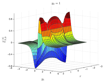
Figure 15: (Color online) Graph of the function $\tilde{L}^{(4)}_{S,0}(iy_{1},iy_{2},r)$ given in Eq. (208) for $y_{2}=1$ as a function of $y_{1}$ and $r=p_{1}/p_{2}$.

Appendix D Functional renormalization group equation for the irreducible polarization

In this appendix we shall derive a formally exact functional renormalization group (FRG) equation for the irreducible polarization which can be used to generate a perturbative expansion of the polarization in powers of bosonic loops with either the RPA interaction or the true effective interaction as propagators. We use the momentum-transfer cutoff scheme proposed in Ref. [Schuetz05, ], where only the free bosonic part $S_{0}[\phi]$ is regularized by suppressing bosonic fluctuations with momenta $q$ smaller than a certain cutoff $\Lambda$. One possibility is to introduce the cutoff as a multiplicative $\Theta$-function Morris94 by replacing in Eq. (45)

$$f_{q}\rightarrow\Theta(q_{0}>|q|>\Lambda)f_{q},$$ (212)

where $\Theta(X)=1$ if the logical expression $X$ is true, and $\Theta(X)=0$ if $X$ is wrong. Alternatively, we may insert an additive cutoff $R_{\Lambda}(q)$ in the inverse propagator Wetterich93 ,

$$f^{-1}_{q}\rightarrow f_{q}^{-1}+R_{\Lambda}(q),$$ (213)

where $R_{\Lambda}(q)=\nu_{0}R(q^{2}/\Lambda^{2})$ with $R(0)=1$ and $R(\infty)=0$. A convenient choice is the Litim regulator $R(x)=(1-x)\Theta(1-x)$, see Ref. [Litim01, ]. All correlation functions then depend on the cutoff $\Lambda$. Denoting the flowing irreducible polarization by $\Pi_{\Lambda}(Q)$, the true irreducible polarization of our model is recovered in the limit $\lim_{\Lambda\rightarrow 0}\Pi_{\Lambda}(Q)=\Pi_{\ast}(Q)$. An exact hierarchy of FRG flow equations for the one-line irreducible vertices of our model can then be obtained by differentiating the corresponding generating functional $\Gamma_{\Lambda}[\langle\bar{c}\rangle,\langle c\rangle,\langle\phi\rangle]$ with respect to $\Lambda$ and expanding $\Gamma_{\Lambda}$ in powers of the expectation values of the fields. A slight complication arises from the fact that even in the absence of external sources the bosonic field $\phi_{Q}$ has a finite expectation value $\phi^{0}_{Q}$, so that for finite external sources

$$\langle\phi_{Q}\rangle=\phi_{Q}^{0}+\delta\phi_{Q}.$$ (214)

In our model, the vacuum expectation value $\phi_{Q}^{0}$ in the absence of sources is related to the exact density $\rho=\int_{K}\langle\bar{c}_{K}c_{K}\rangle$ via the Poisson equation Schuetz06 ,

$$\phi_{Q}^{0}=\delta_{Q,0}\bar{\phi}\;\;,\;\;\bar{\phi}=-if_{0}\rho,$$ (215)

where $\delta_{Q,0}=\beta V\delta_{\bar{\omega},0}\delta_{q,0}$. The one-line irreducible vertices can then be defined by expanding the generating functional $\Gamma_{\Lambda}[\langle\bar{c}\rangle,\langle c\rangle,\langle\phi\rangle]$ in powers of the expectation values $\bar{\psi}=\langle\bar{c}\rangle$, $\psi=\langle{c}\rangle$, and $\delta\phi=\langle\phi\rangle-\phi^{0}$,

$$\Gamma_{\Lambda}[\bar{\psi},\psi,\phi^{0}+\delta\phi] = \sum_{n=0}^{\infty}\sum_{m=0}^{\infty}\frac{1}{(m!)^{2}n!}\int_{K_{1}^{\prime}}\dots\int_{K_{m}^{\prime}}\int_{K_{1}}\dots\int_{K_{m}}\int_{Q_{1}}\dots\int_{Q_{n}}\delta_{K^{\prime}_{1}+\ldots+K^{\prime}_{m},K_{1}+\ldots+K_{m}+Q_{1}+\ldots+Q_{n}}$$ (216)

$$\times \Gamma_{\Lambda}^{(2m,n)}(K^{\prime}_{1},\dots,K^{\prime}_{m};K_{1},\dots,K_{m};Q_{1},\dots,Q_{n})\bar{\psi}_{K^{\prime}_{1}}\cdots\bar{\psi}_{K^{\prime}_{m}}\psi_{K_{1}}\cdots\psi_{K_{m}}\delta\phi_{Q_{1}}\cdots\delta\phi_{Q_{n}}\,.$$

Note that the vertices $\Gamma^{(2m,n)}_{\Lambda}$ implicitly depend on the vacuum expectation value $\bar{\phi}$. Following Ref. [Schuetz06, ], it is convenient to include to contribution $(2\beta Vf_{0})^{-1}(\delta\phi_{0})^{2}$ arising from the fluctuation of the zero mode in the Gaussian part of the bosonic action (45) into the definition of the irreducible vertex $\Gamma^{(0,2)}_{\Lambda}(-Q,Q)$ with two external bosonic legs, so that

$$\Gamma^{(0,2)}_{\Lambda}(-Q,Q)=(\beta V)^{-1}\delta_{Q,0}f_{0}^{-1}+\Pi_{\Lambda}(Q).$$ (217)

The flowing irreducible polarization $\Pi_{\Lambda}(Q)$ then satisfies the exact flow equation Schuetz05 ; Schuetz06 ,

$$\partial_{\Lambda}\Pi_{\Lambda}(Q) = \frac{1}{2}\int_{{Q^{\prime}}}\dot{F}_{\Lambda}({Q}^{\prime})\Gamma^{(4)}_{\Lambda}({Q}^{\prime},-{Q}^{\prime},{Q},-Q)+\Gamma^{(3)}_{\Lambda}(Q,-Q,0)\partial_{\Lambda}\bar{\phi}_{\Lambda}$$ (218)

$$- \int_{Q^{\prime}}\dot{F}_{\Lambda}({Q}^{\prime})F_{\Lambda}(Q+{Q}^{\prime})\Gamma^{(3)}_{\Lambda}(-{Q},{Q}+{Q}^{\prime},-{Q}^{\prime})\Gamma^{(3)}_{\Lambda}({Q}^{\prime},-{Q}-{Q}^{\prime},{Q}).$$

Here for a sharp momentum-transfer cutoff the bosonic propagator is

$${F}_{\Lambda}({Q})=\Theta(q_{0}>|q|>\Lambda)\frac{f_{q}}{1+f_{q}\Pi_{\Lambda}(Q)},$$ (219)

and the corresponding single-scale propagator is

$$\dot{F}_{\Lambda}({Q})=-\delta(|q|-\Lambda)\frac{f_{q}}{1+f_{q}\Pi_{\Lambda}(Q)}.$$ (220)

Alternatively, if we work with a smooth additive cutoff then

$${F}_{\Lambda}({Q})=\frac{f_{q}}{1+f_{q}[\Pi_{\Lambda}(Q)+R_{\Lambda}(q)]},$$ (221)

and

$$\dot{F}_{\Lambda}({Q})=[-\partial_{\Lambda}R_{\Lambda}(q)][{F}_{\Lambda}({Q})]^{2}.$$ (222)

The vertices

$$\Gamma^{(n)}_{\Lambda}(Q_{1},\ldots,Q_{n})\equiv\Gamma^{(0,n)}_{\Lambda}(Q_{1},\ldots,Q_{n})$$ (223)

are the totally symmetrized one-interaction-line irreducible vertices with $n$ external bosonic legs. A graphical representation of Eq. (218) is shown in Fig. 16.

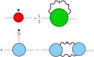
Figure 16: (Color online) Graphical representation of the exact FRG flow equation (218) for the irreducible polarization in the momentum-transfer cutoff scheme. The shaded circles represent the one-interaction-line irreducible vertices, the thick wavy lines denote the exact cutoff-dependent boson propagator (effective interaction) defined in Eq. (219), the small crossed circle is the flowing vacuum expectation value of the bosonic field $\phi$, and the small black dot denotes the derivative with respect to the flow parameter $\Lambda$. The slashed wavy lines represent the single-scale propagator given in Eqs. (220,222).

The flow of the vacuum expectation value $\bar{\phi}_{\Lambda}$ of the bosonic field is determined by the exact FRG equation Schuetz06

$$[f_{0}^{-1}+\Pi_{\Lambda}(0)]\partial_{\Lambda}\bar{\phi}_{\Lambda}=-\frac{1}{2}\int_{Q^{\prime}}\dot{F}_{\Lambda}({Q}^{\prime})\Gamma^{(3)}_{\Lambda}({Q}^{\prime},-{Q}^{\prime},0),$$ (224)

which follows from the requirement that the FRG does not generate any tadpole vertices with only one external bosonic leg. A graphical representation of Eq. (224) is shown in Fig. 17.

Figure 17: (Color online) Graphical representation of the exact FRG flow equation (218) for the vacuum expectation value of the bosonic Hubbard-Stratonovich field. The symbols are explained in the caption of Fig. 16.

We may use Eq. (224) to eliminate the derivative of the flowing vacuum expectation value in the flow equation (218) to obtain the following exact FRG flow equation for the irreducible polarization

$$\partial_{\Lambda}\Pi_{\Lambda}(Q) = \frac{1}{2}\int_{{Q^{\prime}}}\dot{F}_{\Lambda}({Q}^{\prime})\Gamma^{(4)}_{\Lambda}({Q}^{\prime},-{Q}^{\prime},{Q},-Q)-\frac{1}{2}\frac{f_{0}}{1+f_{0}\Pi_{\Lambda}(0)}\Gamma^{(3)}_{\Lambda}(Q,-Q,0)\int_{Q^{\prime}}\dot{F}_{\Lambda}({Q}^{\prime})\Gamma^{(3)}_{\Lambda}({Q}^{\prime},-{Q}^{\prime},0)$$ (225)

$$- \int_{Q^{\prime}}\dot{F}_{\Lambda}({Q}^{\prime})F_{\Lambda}(Q+{Q}^{\prime})\Gamma^{(3)}_{\Lambda}(-{Q},{Q}+{Q}^{\prime},-{Q}^{\prime})\Gamma^{(3)}_{\Lambda}({Q}^{\prime},-{Q}-{Q}^{\prime},{Q}).$$

As shown in Ref. [Schuetz05, ] (see also the appendix of the first work cited in Ref. [Schuetz06, ] for a formal proof), in the momentum-transfer cutoff scheme the vertices at the initial scale $\Lambda=\Lambda_{0}\equiv q_{0}$ satisfy non-trivial initial conditions. The requirement that the vertex $\Gamma^{(0,1)}_{\Lambda_{0}}$ with one bosonic leg vanishes at $\Lambda=\Lambda_{0}$ implies that the fermionic self-energy $\Sigma_{\Lambda_{0}}(K)=\Gamma_{\Lambda_{0}}^{(2,0)}(K,K)$ at the initial scale is given by the self-consistent Hartree approximation,

$$\Sigma_{\Lambda_{0}} = f_{0}\rho_{0},$$ (226)

where the initial density $\rho_{0}$ satisfies the Hartree self-consistency condition (58). The initial conditions for the purely bosonic vertices $\Gamma^{(0,n)}_{\Lambda_{0}}\equiv\Gamma^{(n)}_{\Lambda_{0}}$ are for $n=2$,

$$\Gamma^{(0,2)}_{\Lambda_{0}}(-Q,Q)=(\beta V)^{-1}\delta_{Q,0}f_{0}^{-1}-L^{(2)}_{S}(Q,-Q),$$ (227)

and for $n>2$,

$$\Gamma^{(0,n)}_{\Lambda_{0}}(Q_{1},\ldots,Q_{n})=i^{n}(n-1)!\;L^{(n)}_{S}(-Q_{1},\ldots,-Q_{n}),$$ (228)

where $L^{(n)}_{S}(Q_{1},\ldots,Q_{n})$ are the symmetrized closed fermion loops with $n$ external legs defined in Eq. (174). A graphical representation of Eq. (228) is shown in Fig. 5. By definition, the symmetrized two-loop is (up to a minus sign) given by the non-interacting polarization $\Pi_{0}(Q)$,

$$L^{(2)}_{S}(-Q,Q)=\int_{K}G_{0}(K)G_{0}(K+Q)=-\Pi_{0}(Q).$$ (229)

However, in contrast to Eq. (18), the fermionic Green functions in Eq. (229) are self-consistent Hartree Green functions as defined in Eq. (59). Finally, in the momentum-transfer cutoff scheme the initial value of the three-legged vertex $\Gamma^{(2,1)}_{\Lambda_{0}}(K^{\prime};K;Q)$ is

$$\Gamma^{(2,1)}_{\Lambda_{0}}(K^{\prime};K;Q)=i,$$ (230)

which follows from Eq. (46). All other vertices vanish at the initial scale $\Lambda=\Lambda_{0}$.

The above RG equation (225) is exact but not closed, and should be augmented by FRG flow equations for the vertices $\Gamma^{(3)}_{\Lambda}$ and $\Gamma^{(4)}_{\Lambda}$, which in turn involve higher order bosonic vertices. Only for linearized energy dispersion the closed loop theorem guarantees that $\Gamma^{(n)}_{\Lambda}(Q_{1},\ldots,Q_{n})=0$, so that we recover the well-known result that the RPA is exact for the Tomonaga-Luttinger model. To motivate a sensible truncation procedure for quadratic energy dispersion, we note that the vertices $\Gamma^{(n)}_{\Lambda}$ with $n\geq 3$ are irrelevant in the renormalization group sense: If we assign to the momentum-independent part of the interaction $f_{0}=f_{q=0}$ a vanishing scaling dimension, then in $D$ dimensions the vertices $\Gamma_{\Lambda}^{(n)}$ have scaling dimensions $-(D+z_{\phi})(n/2-1)$, where $z_{\phi}$ is the dynamic exponent of the bosonic field mediating the forward scattering interaction. In one dimension $z_{\phi}=1$ due to the linear dispersion of the ZS mode, so that in $D=1$ the vertex $\Gamma^{(3)}$ is irrelevant with scaling dimension $-1$, while $\Gamma^{(4)}$ is irrelevant with scaling dimension $-2$. Because the renormalization group flow of irrelevant couplings is usually not important, it is reasonable to truncate the infinite hierarchy of flow equations by approximating the vertices $\Gamma^{(3)}_{\Lambda}$ and $\Gamma^{(4)}_{\Lambda}$ in Eq. (218) by their initial values at $\Lambda=\Lambda_{0}$,

$$\Gamma^{(n)}_{\Lambda}(Q_{1},\ldots,Q_{n}) \approx \Gamma^{(n)}_{\Lambda_{0}}(Q_{1},\ldots,Q_{n})$$ (231)

$$=i^{n}(n-1)!L^{(n)}_{S}(-Q_{1},\ldots,-Q_{n}),$$

where the symmetrized closed fermion loops are defined in Eq. (174). In particular, for the vertices appearing in Eq. (225) we substitute

$$\Gamma^{(3)}_{\Lambda}(Q_{1},Q_{2},-Q_{1}-Q_{2})$$ (232)

$$\rightarrow-2iL^{(3)}_{S}(-Q_{1},-Q_{2},Q_{1}+Q_{2}),$$

$$\Gamma^{(4)}_{\Lambda}(Q_{1},-Q_{1},Q_{2},-Q_{2})$$ (233)

$$\rightarrow 6L^{(4)}_{S}(-Q_{1},Q_{1},-Q_{2},Q_{2}).$$

Then Eq. (225) becomes a closed integro-differential equation for $\Pi_{\Lambda}(Q)$, the solution of which gives for $\Lambda\rightarrow 0$ a non-perturbative estimate for the irreducible polarization. We can easily recover from (225) the perturbative expansion (67) of the irreducible polarization $\Pi_{\ast}(Q)$ in powers of the RPA interaction if we replace the flowing polarization on the right-hand side of Eq. (225) by the non-interacting one, $\Pi_{\Lambda}(Q)\rightarrow\Pi_{0}(Q)$, which amounts to replacing the flowing effective interaction in $F_{\Lambda}(Q)$ by the RPA interaction defined in Eq. (66). With these substitutions, it is easy to integrate both sides of Eq. (225) over the flow parameter $\Lambda$ and recover Eq. (67). Alternatively, we may truncate Eq. (225) by replacing the flowing polarization on the right-hand side by its limiting value without cutoff, $\Pi_{\ast}(Q)=\lim_{\Lambda\rightarrow 0}\Pi_{\Lambda}(Q)$. Then we arrive that the one-loop self-consistency equation for $\Pi_{\ast}(Q)$ given in Eqs. (79–83).

Note that even with the truncation (232,233) the FRG flow equation (225) is non-perturbative, because the renormalization of the polarization is self-consistently taken into account in the bosonic loop integrations. It should be interesting to analyze Eq. (225) numerically and try to extract the spectral line-shape. Possibly, one can check in this way whether the resummation procedure proposed by Pustilnik et al. Pustilnik06 is justified also for non-integrable models.

References

- (1) K. V. Samokhin, J. Phys.: Cond. Mat. 10, L533 (1998).
- (2) F.Capurro, M. Polini, and M. P. Tosi, Physica B 325, 287 (2003).
- (3) M. Pustilnik, E. G. Mishchenko, L. I. Glazman, and A. V. Andreev, Phys. Rev. Lett. 91, 126805, (2003).
- (4) M. Pustilnik, M. Khodas, A. Kamenev, and L. I. Glazman, Phys. Rev. Lett. 96, 196405 (2006).
- (5) M. Pustilnik, Phys. Rev. Lett. 97, 036404 (2006).
- (6) V. V. Cheianov and M. Pustilnik, arXiv:0710.3589v1.
- (7) S. Teber, Eur. Phys. J. B 52, 233 (2006).
- (8) S. Teber, Phys. Rev. B 76, 045309 (2007).
- (9) R. G. Pereira, J. Sirker, J.-S. Caux, R. Hagemans, J. M. Maillet, S. R. White, and I. Affleck, Phys. Rev. Lett. 96, 257202 (2006).
- (10) R. G. Pereira, J. Sirker, J.-S. Caux, R. Hagemans, J. M. Maillet, S. R. White, and I. Affleck, J. Stat. Mech. P08022 (2007).
- (11) R. G. Pereira, S. R. White, and I. Affleck, Phys. Rev. Lett. 100, 027206 (2008).
- (12) P. Pirooznia and P. Kopietz, Eur. Phys. J. B 58, 291 (2007).
- (13) K. Schönhammer, Phys. Rev. B 75, 205103 (2007).
- (14) D. N. Aristov, Phys. Rev. B 76, 085327 (2007).
- (15) P. Plötz, arXiv:0708.1424v1.
- (16) D. Pines and P. Nozières, The Theory of Quantum Liquids, (Addison-Wesley Advanced Book Classics, Redwood City, CA, 1989).
- (17) We focus on neutral spinless fermions in this work. In charged Fermi systems the ZS mode becomes the plasmon Pines89 .
- (18) J. Solyom, Adv. Phys. 28, 201 (1979).
- (19) F. D. M. Haldane, J.Phys. C 14, 2585 (1981).
- (20) T. Giamarchi, Quantum Physics in One Dimension, (Clarendon Press, Oxford, 2004).
- (21) K. Schönhammer, in Interacting Electrons in Low Dimensions, Ed.: D. Baeriswyl and L. Degeorgi, (Kluwer, Dordrecht, 2005).
- (22) M. Schick, Phys. Rev. 166, 404 (1968).
- (23) H. C. Fogedby, J. Phys. C 9, 3757 (1976).
- (24) D. K. K. Lee and Y. Chen, J. Phys. A 21, 4155 (1988).
- (25) P. Kopietz and K. Schönhammer, Z. Phys. B 100, 259 (1996); P. Kopietz, J. Hermisson, and K. Schönhammer, Phys. Rev. B 52, 10877 (1995).
- (26) P. Kopietz and G. E. Castilla, Phys. Rev. Lett. 76, 4777 (1996); T. Busche and P. Kopietz, Int. J. Mod. Phys. B14, 1481 (2000).
- (27) P. Kopietz, Bosonization of interacting fermions in arbitrary dimensions, (Springer, Berlin, 1997; cond-mat/0605402).
- (28) A. Neumayr and W. Metzner, Phys. Rev. B 58, 15449 (1998).
- (29) A. Neumayr and W. Metzner, J. Stat. Phys. 96, 613 (1999).
- (30) C. Kopper and J. Magnen, Ann. Henri Poincaré 2, 513 (2001).
- (31) A. V. Chubukov, D. L. Maslov, and R. Saha, arXiv:0707.4422v2; A. V. Chubukov, D. L. Maslov, and F. H. L. Essler, arXiv:0801.1837v1.
- (32) I. E. Dzyaloshinskii and A. I. Larkin, Zh. Eksp. Teor. Fiz. 65, 411 (1973) [Sov. Phys. JETP 38, 202 (1974)].
- (33) W. Metzner, C. Castellani, and C. Di Castro, Adv. Phys. 47, 3 (1998).
- (34) There is a printing error in the expression for given in Eq. (6) of Ref. [Pirooznia07, ]; the correct result for is given in Eq. (LABEL:eq:dispersion) of the present work.
- (35) In three dimensions, the single particle-hole pair continuum is within RPA smeared out over a frequency interval , while the collective ZS mode lies (for repulsive interactions) above the upper limit of the single-pair continuum Pines89 . More generally, in arbitrary dimensions and for repulsive short-range interactions the long-wavelength dispersion of the ZS mode is with .
- (36) F. Schütz, L. Bartosch, and P. Kopietz, Phys. Rev. B 72, 035107 (2005).
- (37) F. Schütz and P. Kopietz, J. Phys. A: Math. Gen. 39, 8205 (2006); A. Sinner, N. Hasselmann, and P. Kopietz, arXiv:0707.4110 (J. Phys.: Condens. Matter 20, 2008).
- (38) A. Neumayr and W. Metzner, Phys. Rev. B 67, 035112 (2003).
- (39) S. Ledowski and P. Kopietz, J. Phys.: Condens. Matter 15, 4779 (2003).
- (40) The three-loop appearing in the Hartree-type-of contribution (83) to the irreducible polarization is ambiguous for the required combination of arguments. Because Hartree interactions should be static, we define as the limit of where we first set the frequency sum equal to zero and then take the limit .
- (41) We thank F. H. L. Essler for pointing this out to us.
- (42) T. R. Morris, Int. J. Mod. Phys. A 9, 2411 (1994).
- (43) C. Wetterich, Phys. Lett. B 301, 90 (1993); J. Berges, N. Tetradis, and C. Wetterich, Phys. Rep. 363, 223 (2002).
- (44) D. Litim, Phys. Rev. D 64, 105007 (2001).