Existence of non-trivial harmonic functions
on Cartan-Hadamard manifolds
of unbounded curvature

Abstract.

The Liouville property of a complete Riemannian manifold $M$ (i.e., the question whether there exist non-trivial bounded harmonic functions on $M$) attracted a lot of attention. For Cartan-Hadamard manifolds the role of lower curvature bounds is still an open problem. We discuss examples of Cartan-Hadamard manifolds of unbounded curvature where the limiting angle of Brownian motion degenerates to a single point on the sphere at infinity, but where nevertheless the space of bounded harmonic functions is as rich as in the non-degenerate case. To see the full boundary the point at infinity has to be blown up in a non-trivial way. Such examples indicate that the situation concerning the famous conjecture of Greene and Wu about existence of non-trivial bounded harmonic functions on Cartan-Hadamard manifolds is much more complicated than one might have expected.

1. Introduction

The study of harmonic functions on complete Riemannian manifolds, i.e., the solutions of the equation $\Delta u=0$ where $\Delta$ is the Laplace-Beltrami operator, lies at the interface of analysis, geometry and stochastics. Indeed, there is a deep interplay between geometry, harmonic function theory, and the long-term behaviour of Brownian motion. Negative curvature amplifies the tendency of Brownian motion to move away from its starting point and, if topologically possible, to wander out to infinity. On the other hand, non-trivial asymptotic properties of Brownian paths for large time correspond with non-trivial bounded harmonic functions on the manifold.

There is plenty of open questions concerning the richness of certain spaces of harmonic functions on Riemannian manifolds. Even in the case of simply connected negatively curved Riemannian manifolds basic questions are still open. For instance, there is not much known about the following problem posed by Wu in 1983.

Question 1.1 (cf. Wu [27] p. 139).

If $M$ is a simply-connected complete Riemannian manifold with sectional curvature $\leq{-c}<0$, do there exist $n$ bounded harmonic functions ($n=\dim M$) which give global coordinates on $M$?

It should be remarked that, under the given assumptions, it is even not known in general whether there exist non-trivial bounded harmonic functions at all. This question is the content of the famous Greene-Wu conjecture which asserts existence of non-constant bounded harmonic functions under slightly more precise curvature assumptions.

Conjecture 1.2 (cf. Greene-Wu [10] p. 767).

Let $M$ be a simply-connected complete Riemannian manifold of non-positive sectional curvature and $x_{0}\in M$ such that

$$\hbox{\rm Sect}^{M}_{x}\leq-c\,r(x)^{-2}\quad\text{for all }\,x\in M\setminus K$$

for some $K$ compact, $c>0$ and $r=\hbox{\rm dist}(x_{0},{\kern 0.8pt\cdot\kern 0.8pt})$. Then $M$ carries non-constant bounded harmonic functions.

Concerning Conjecture 1.2 substantial progress has been made since the pioneering work of Anderson [3], Sullivan [3], and Anderson-Schoen [4]. Nevertheless, the role of lower curvature bounds is far from being understood.

From a probabilistic point of view, Conjecture 1.2 concerns the eventual behaviour of Brownian motion on these manifolds as time goes to infinity. Indeed, for any Riemannian manifold, we have the following probabilistic characterization.

Lemma 1.3.

For a Riemannian manifold $(M,g)$ the following two conditions are equivalent:

1. There exist non-constant bounded harmonic functions on $M$.

2. BM has non-trivial exit sets, i.e., if $X$ is a Brownian motion on $M$ then there exist open sets $U$ in the $1$-point compactification $\hat{M}$ of $M$ such that

   $$\mathbb{P}\{X_{t}\in U\hbox{\ eventually}\}\not=0\hbox{\ or\ }1.$$

More precisely, Brownian motion $X$ on $M$ may be realized on the space $C(\mathbb{R}_{+},\hat{M})$ of continuous paths with values in the $1$-point compactification $\hat{M}$ of $M$, equipped with the standard filtration ${\mathscr{F}}_{t}=\sigma\{X_{s}=\mathop{\mathchoice{\text{\rm pr}}{\text{\rm pr}}{\text{\rm pr}}{\text{\rm pr}}}\nolimits_{s}|s\leq t\}$ generated by the coordinate projections $\mathop{\mathchoice{\text{\rm pr}}{\text{\rm pr}}{\text{\rm pr}}{\text{\rm pr}}}\nolimits_{s}$ up to time $t$. Let $\zeta=\sup\{t>0:X_{t}\in M\}$ be the lifetime of $X$ and let ${\mathscr{F}}_{\hbox{\sevenrm inv}}$ denote the shift-invariant $\sigma$-field on $C(\mathbb{R}_{+},\tilde{M})$. Then there is a canonical isomorphism between the space ${\mathscr{H}}_{\hbox{\sevenrm b}}(M)$ of bounded harmonic functions on $M$ and the set $b{\mathscr{F}}_{\hbox{\sevenrm inv}}$ of bounded ${\mathscr{F}}_{\hbox{\sevenrm inv}}$-measurable random variables up to equivalence, given as follows:

(1.1) $${\mathscr{H}}_{\hbox{\sevenrm b}}(M)\mathrel{\mathchoice{\lower 0.5pt\vbox{\halign{$\m@th\displaystyle\hfil#\hfil$\cr\sim\crcr\longrightarrow\crcr}}}{\lower 0.5pt\vbox{\halign{$\m@th\textstyle\hfil#\hfil$\cr\sim\crcr\longrightarrow\crcr}}}{\lower 0.5pt\vbox{\halign{$\m@th\scriptstyle\hfil#\hfil$\cr\sim\crcr\longrightarrow\crcr}}}{\lower 0.5pt\vbox{\halign{$\m@th\scriptscriptstyle\hfil#\hfil$\cr\sim\crcr\longrightarrow\crcr}}}}b{\mathscr{F}}_{\hbox{\sevenrm inv}}/_{\sim},\quad u\longmapsto\lim_{t\uparrow\zeta}(u\circ X_{t}).$$

(Bounded shift-invariant random variables are considered as equivalent, if they agree $\mathbb{P}_{x}$-a.e., for each $x\in M$.) Note that the isomorphism (1.1) is well defined by the martingale convergence theorem, and that the inverse map to (1.1) is given by taking expectations:

(1.2) $$b{\mathscr{F}}_{\hbox{\sevenrm inv}}/_{\sim}\ni H\longmapsto u\in{\mathscr{H}}_{\hbox{\sevenrm b}}(M)\ \text{ where }u(x):=\mathbb{E}_{x}[H].$$

In particular,

$$u(x):=\mathbb{P}_{x}\{X_{t}\in U\hbox{\ eventually}\}$$

is a bounded harmonic function on $M$, and non-constant if and only if $U$ is a non-trivial exit set.

Now let $(M,g)$ be a Cartan-Hadamard manifold, i.e., a simply connected complete Riemannian manifold of non-positive sectional curvature. (All manifolds are supposed to be connected). In terms of the exponential map $\exp_{x_{0}}\colon T_{x_{0}}M\mathrel{\mathchoice{\lower 0.5pt\vbox{\halign{$\m@th\displaystyle\hfil#\hfil$\cr\sim\crcr\longrightarrow\crcr}}}{\lower 0.5pt\vbox{\halign{$\m@th\textstyle\hfil#\hfil$\cr\sim\crcr\longrightarrow\crcr}}}{\lower 0.5pt\vbox{\halign{$\m@th\scriptstyle\hfil#\hfil$\cr\sim\crcr\longrightarrow\crcr}}}{\lower 0.5pt\vbox{\halign{$\m@th\scriptscriptstyle\hfil#\hfil$\cr\sim\crcr\longrightarrow\crcr}}}}M$ at a fixed base point $x_{0}\in M$, we identify $\rho\colon\mathbb{R}^{n}\cong T_{x_{0}}M\mathrel{\mathchoice{\lower 0.5pt\vbox{\halign{$\m@th\displaystyle\hfil#\hfil$\cr\sim\crcr\longrightarrow\crcr}}}{\lower 0.5pt\vbox{\halign{$\m@th\textstyle\hfil#\hfil$\cr\sim\crcr\longrightarrow\crcr}}}{\lower 0.5pt\vbox{\halign{$\m@th\scriptstyle\hfil#\hfil$\cr\sim\crcr\longrightarrow\crcr}}}{\lower 0.5pt\vbox{\halign{$\m@th\scriptscriptstyle\hfil#\hfil$\cr\sim\crcr\longrightarrow\crcr}}}}M$. Via pullback of the metric on $M$, we get an isometric isomorphism $(M,g)\cong(\mathbb{R}^{n},\rho^{*}g)$, and in particular, $M\setminus\{x_{0}\}\cong{]0,\infty[}\times S^{n-1}$. In terms of such global polar coordinates, Brownian motions $X$ on $M$ may be decomposed into their radial and angular part,

$$X_{t}=(r(X_{t}),\vartheta(X_{t}))$$

where $r(X_{t})=\mathop{\mathchoice{\text{\rm dist}}{\text{\rm dist}}{\text{\rm dist}}{\text{\rm dist}}}\nolimits(x_{0},X_{t})$ and where $\vartheta(X_{t})$ takes values in $S^{n-1}$.

For a Cartan-Hadamard manifold $M$ of dimension $n$ there is a natural geometric boundary, the sphere at infinity $S_{\infty}(M)$, such that $M\cup S_{\infty}(M)$ equipped with the cone topology is homeomorphic to the unit ball $B\subset\mathbb{R}^{d}$ with boundary $\partial B=S^{d-1}$, cf. [9], [5]. In terms of polar coordinates on $M$, a sequence $(r_{n},\vartheta_{n})_{n\in\mathbb{N}}$ of points in $M$ converges to a point of $S_{\infty}(M)$ if and only if $r_{n}\to\infty$ and $\vartheta_{n}\to\vartheta\in S^{n-1}$.

Given a continuous function $f\colon S_{\infty}(M)\to\mathbb{R}$ the Dirichlet problem at infinity is to find a harmonic function $h\colon M\to\mathbb{R}$ which extends continuously to $S_{\infty}(M)$ and there coincides with the given function $f$, i.e.,

$$h|S_{\infty}(M)=f.$$

The Dirichlet problem at infinity is called solvable if this is possible for every such function $f$. In this case a rich class of non-trivial bounded harmonic functions on $M$ can be constructed via solutions of the Dirichlet problem at infinity.

In 1983, Anderson [3] proved that the Dirichlet problem at infinity is indeed uniquely solvable for Cartan-Hadamard manifolds of pinched negative curvature, i.e. for complete simply connected Riemannian manifolds $M$ whose sectional curvatures satisfy

$$-a^{2}\leq\mathop{\mathchoice{\text{\rm Sect}}{\text{\rm Sect}}{\text{\rm Sect}}{\text{\rm Sect}}}\nolimits^{M}_{x}\leq-b^{2}\text{ for all $x\in M$,}$$

where $a^{2}>b^{2}>0$ are arbitrary constants. The proof uses barrier functions and Perron’s classical method to construct harmonic functions. Along the same ideas Choi [7] showed in 1984 that in rotational symmetric case of a model $(M,g)$ the Dirichlet problem at infinity is solvable if the radial curvature is bounded from above by $-A/(r^{2}\log(r))$. Hereby a Riemannian manifold $(M,g)$ is called model if it possesses a pole $p\in M$ and every linear isometry $\varphi\colon T_{p}M\to T_{p}M$ can be realized as the differential of an isometry $\Phi\colon M\to M$ with $\Phi(p)=p$. Choi [7] furthermore provides a criterion, the convex conic neighbourhood condition, which is sufficient for solvability of the Dirichlet problem at infinity.

Definition 1.4 (cf. Choi [7]).

A Cartan-Hadamard manifold $M$ satisfies the convex conic neighbourhood condition at $x\in S_{\infty}(M)$ if for any $y\in S_{\infty}(M)$, $y\not=x$, there exist subsets $V_{x}$ and $V_{y}\subset M\cup S_{\infty}(M)$ containing $x$ and $y$ respectively, such that $V_{x}$ and $V_{y}$ are disjoint open sets of $M\cup S_{\infty}(M)$ in terms of the cone topology and $V_{x}\cap M$ is convex with ${C}^{2}$-boundary. If this condition is satisfied for all $x\in S_{\infty}(M)$, $M$ is said to satisfy the convex conic neighbourhood condition.

It is shown in Choi [7] that the Dirichlet problem at infinity is solvable for a Cartan-Hadamard manifold $M$ with sectional curvature bounded from above by $-c^{2}$ for some $c>0$, if $M$ satisfies the convex conic neighbourhood condition.

In probabilistic terms, if the Dirichlet problem at infinity for $M$ is solvable and almost surely

$$X_{\zeta}:=\lim_{t\to\zeta}X_{t}$$

exists in $S_{\infty}(M)$, where $(X_{t})_{t<\zeta}$ is a Brownian motion on $M$ with lifetime $\zeta$, the unique solution $h\colon M\to\mathbb{R}$ to the Dirichlet problem at infinity with boundary function $f$ is given as

(1.3) $$h(x)=\mathbb{E}\left[f\circ X_{\zeta(x)}(x)\right].$$

Here $X(x)$ is a Brownian motion starting at $x\in M$.

Conversely, supposing that for Brownian motion $X(x)$ on $M$ almost surely

$$\lim_{t\to\zeta(x)}X_{t}(x)$$

exists in $S_{\infty}(M)$ for each $x\in M$, one may consider the harmonic measure $\mu_{x}$ on $S_{\infty}(M)$, where for a Borel set $U\subset S_{\infty}(M)$

(1.4) $$\mu_{x}(U):=\mathbb{P}\left\{X_{\zeta(x)}(x)\in U\right\}.$$

Then, for any Borel set $U\subset S_{\infty}(M)$, the assignment

$$x\mapsto\mu_{x}(U)$$

defines a bounded harmonic function $h_{U}$ on $M$. By the maximum principle $h_{U}$ is either identically equal to $0$ or $1$ or takes its values in $]0,1[$. Furthermore, all harmonic measures $\mu_{x}$ on $S_{\infty}(M)$ are equivalent. Thus, by showing that the harmonic measure class on $S_{\infty}(M)$ is non-trivial, we can construct non-trivial bounded harmonic functions on $M$. To show that, for a given continuous boundary function $f\colon S_{\infty}(M)\to\mathbb{R}$, the harmonic function

(1.5) $$h(x)=\int_{S_{\infty}(M)}f(y)\mu_{x}(dy).$$

extends continuously to the boundary $S_{\infty}(M)$ and takes there the prescribed boundary values $f$, we have to show that, whenever a sequence of points $x_{i}$ in $M$ converges to $x_{\infty}\in S_{\infty}(M)$ then the measures $\mu_{x_{i}}$ converge weakly to the Dirac measure at $x_{\infty}$. In particular, for a continuous boundary function $f|S_{\infty}(M)$, the unique solution to the Dirichlet problem at infinity is given by formula (1.5).

The first results in this direction have been obtained by Prat [24, 25] between 1971 and 1975. He proved that on a Cartan-Hadamard manifold with sectional curvature bounded from above by a negative constant $-k^{2}$, $k>0$, Brownian motion is transient, i.e., almost surely all paths of the Brownian motion exit from $M$ at the sphere at infinity [25]. If in addition the sectional curvatures are bounded from below by a constant $-K^{2}$, $K>k$, he showed that the angular part $\vartheta(X_{t})$ of the Brownian motion almost surely converges as $t\to\zeta$.

In 1976, Kifer [17] presented a stochastic proof that on Cartan-Hadamard manifolds with sectional curvature pinched between two strictly negative constants and satisfying a certain additional technical condition, the Dirichlet problem at infinity can be uniquely solved. The proof there was given in explicit terms for the two dimensional case. The case of a Cartan-Hadamard manifold $(M,g)$ with pinched negative curvature without additional conditions and arbitrary dimension was finally treated in Kifer [18].

Independently of Anderson, in 1983, Sullivan [26] gave a stochastic proof of the fact that on a Cartan-Hadamard manifold with pinched negative curvature the Dirichlet problem at infinity is uniquely solvable. The crucial point has been to prove that the harmonic measure class is non-trivial in this case.

Theorem 1.5 (Sullivan [26]).

The harmonic measure class on $S_{\infty}(M)=\partial(M\cup S_{\infty}(M))$ is positive on each non-void open set. In fact, if $x_{i}$ in $M$ converges to $x_{\infty}$ in $S_{\infty}(M)$, then the Poisson hitting measures $\mu_{x_{i}}$ tend weakly to the Dirac mass at $x_{\infty}$.

In the special case of a Riemannian surface $M$ of negative curvature bounded from above by a negative constant, Kendall [16] gave a simple stochastic proof that the Dirichlet problem at infinity is uniquely solvable. He thereby used the fact that every geodesic on the Riemannian surface “joining” two different points on the sphere at infinity divides the surface into two disjoint half-parts. Starting from a point $x$ on $M$, with non-trivial probability Brownian motion will eventually stay in one of the two half-parts up to its lifetime. As this is valid for every geodesic and every starting point $x$, the non-triviality of the harmonic measure class on $S_{\infty}(M)$ follows.

Concerning the case of Cartan-Hadamard manifolds of arbitrary dimension several results have been published how the pinched curvature assumption can be relaxed such that still the Dirichlet problem at infinity for $M$ is solvable, e.g. [14] and [12].

Theorem 1.6 (Hsu [12]).

Let $(M,g)$ be a Cartan-Hadamard manifold. The Dirichlet problem at infinity for $M$ is solvable if one of the following conditions is satisfied:

1. There exists a positive constant $a$ and a positive and nonincreasing function $h$ with $\int_{0}^{\infty}rh(r)\,dr<\infty$ such that

   $$-h(r(x))^{2}e^{2ar(x)}\leq\mathop{\mathchoice{\text{\rm Ric}}{\text{\rm Ric}}{\text{\rm Ric}}{\text{\rm Ric}}}\nolimits^{M}_{x}\text{ and }\mathop{\mathchoice{\text{\rm Sect}}{\text{\rm Sect}}{\text{\rm Sect}}{\text{\rm Sect}}}\nolimits^{M}_{x}\leq-a^{2}\text{ for all $x\in M$. }$$

2. There exist positive constants $r_{0}$, $\alpha>2$ and $\beta<\alpha-2$ such that

   $$-r(x)^{2\beta}\leq\mathop{\mathchoice{\text{\rm Ric}}{\text{\rm Ric}}{\text{\rm Ric}}{\text{\rm Ric}}}\nolimits^{M}_{x}\text{ and }\mathop{\mathchoice{\text{\rm Sect}}{\text{\rm Sect}}{\text{\rm Sect}}{\text{\rm Sect}}}\nolimits^{M}_{x}\leq-\frac{\alpha(\alpha-1)}{r(x)^{2}}$$

   for all $x\in M$ with $r(x)\geq r_{0}$.

It was an open problem for some time whether the existence of a strictly negative upper bound for the sectional curvature could already be a sufficient condition for the solvability of the Dirichlet problem at infinity as it is true in dimension 2. In 1994 however, Ancona [2] constructed a Riemannian manifold with sectional curvatures bounded above by a negative constant such that the Dirichlet problem at infinity for $M$ is not solvable. For this manifold Ancona discussed the asymptotic behaviour of Brownian motion. In particular, he showed that Brownian motion almost surely exits from $M$ at a single point $\infty_{M}$ on the sphere at infinity. Ancona did not deal with the question whether $M$ carries non-trivial bounded harmonic functions.

Borbély [6] gave another example of a Cartan-Hadamard manifold with curvature bounded above by a strictly negative constant, on which the Dirichlet problem at infinity is not solvable. Borbély does not discuss Brownian motion on this manifold, but he shows using analytic methods that his manifold supports non-trivial bounded harmonic functions.

This paper aims to give a detailed analysis of manifolds of this type and to answer several questions. It turns out that the manifolds of Ancona and Borbély share quite similar properties, at least from the probabilistic point of view. On both manifolds the angular behaviour of Brownian motion degenerates to a single point, as Brownian motion drifts to infinity. In particular, the Dirichlet problem at infinity is not solvable. Nevertheless both manifolds possess a wealth of non-trivial bounded harmonic functions, which come however from completely different reasons than in the pinched curvature case. Since Borbély’s manifold is technical easier to handle, we restrict our discussion to this case. It should however be noted that all essential features can also be found in Ancona’s example.

Unlike Borbély who used methods of partial differential equations to prove that his manifold provides an example of a non-Liouville manifold for that the Dirichlet problem at infinity is not solvable, we are interested in a complete stochastic description of the considered manifold. In this paper we give a full description of the Poisson boundary of Borbély’s manifold by characterizing all shift-invariant events for Brownian motion. The manifold is of dimension 3, and the $\sigma$-algebra of invariant events is generated by two random variables. It turns out that, in order to see the full Poisson boundary, the attracting point at infinity to which all Brownian paths converge needs to be “unfolded” into the $2$-dimensional space $\mathbb{R}\times S^{1}$.

The asymptotic behaviour of Brownian motion on this manifold is in sharp contrast to the case of a Cartan-Hadamard manifold of pinched negative curvature. Recall that in the pinched curvature case the angular part $\vartheta(X)$ of $X$ carries all relevant information and the limiting angle $\lim_{t\to\infty}\vartheta(X_{t})$ generates the shift-invariant $\sigma$-field of $X$. All non-trivial information to distinguish Brownian paths for large times is given in terms of the angular projection of $X$ onto $S_{\infty}(M)$, where only the limiting angle matters. As a consequence, any bounded harmonic function comes from a solution of the Dirichlet problem at infinity, which means on the other hand that any bounded harmonic function on $M$ has a continuous continuation to the boundary at infinity.

More precisely, denoting by $h(M)$ the Banach space of bounded harmonic functions on a Cartan-Hadamard manifold $M$, we have the following result of Anderson.

Theorem 1.7 ([3]).

Let $(M,g)$ be a Cartan-Hadamard manifold of dimension $d$, whose sectional curvatures satisfy $-a^{2}\leq\mathop{\mathchoice{\text{\rm Sect}}{\text{\rm Sect}}{\text{\rm Sect}}{\text{\rm Sect}}}\nolimits^{M}_{x}\leq-b^{2}$ for all $x\in M$. Then the linear mapping

(1.6) $$\begin{split}P\colon L^{\infty}(S_{\infty}(M),\mu)&\to h(M),\\ f&\mapsto P(f),\quad P(f)(x):=\int_{S_{\infty}(M)}fd\mu_{x}\end{split}$$

is a norm-nonincreasing isomorphism onto $h(M)$.

In the situation of Borbély’s manifold Brownian motion almost surely exits from the manifold at a single point of the sphere at infinity, independent of its starting point $x$ at time $0$. In particular, all harmonic measures $\mu_{x}$ are trivial, and harmonic functions of the form $P(f)$ are necessarily constant. On the other hand, we are going to show that this manifold supports a huge variety of non-trivial bounded harmonic functions, necessarily without continuation to the sphere at infinity. It turns out that the richness of harmonic functions is related to two different kinds of non-trivial exit sets for the Brownian motion:

1. Non-trivial shift-invariant information is given in terms of the direction along which Brownian motion approaches the point at the sphere at infinity. Even if there is no contribution from the limiting angle itself, angular sectors about the limit point allow to distinguish Brownian paths for large times.

2. As Brownian motion converges to a single point, in appropriate coordinates the fluctuative components (martingale parts) of Brownian motion for large times are relatively small compared to its drift components. Roughly speaking, this means that for large times Brownian motion follows the integral curves of the deterministic dynamical system which is given by neglecting the martingale components in the describing stochastic differential equations. We show that this idea can be made precise by constructing a deterministic vector field on the manifold $M$ such that the corresponding flow induces a foliation of $M$ and such that Brownian motion exits $M$ asymptotically along the leaves of this foliation.

To determine the Poisson boundary the main problem is then to show that there are no other non-trivial exit sets. This turns out to be the most difficult point and will be done by purely probabilistic arguments using time reversal of Brownian motion. To this end, the time-reversed Brownian motion starting on the exit boundary and running backwards in time is investigated.

It is interesting to note that on the constructed manifold, despite of diverging curvature, the harmonic measure has a density (Poisson kernel) with respect to the Lebesgue measure. Recall that in the pinched curvature case the harmonic measure may well be singular with respect to the surface measure on the sphere at infinity (see [17], [22], [15], [8] for results in this direction). Typically it is the fluctuation of the geometry at infinity which prevents harmonic measure from being absolutely continuous. Pinched curvature alone does in general not allow to control the angular derivative of the Riemannian metric, when written in polar coordinates.

The paper is organized as follows. In Section 2 we give the construction of our manifold $M$ which up to minor technical modifications is the same as in Borbély [6]: we define $M$ as the warped product

$$M:=(H\cup L)\times_{g}S^{1},$$

where $L$ is a unit-speed geodesic in the hyperbolic space $\mathbb{H}^{2}$ of constant sectional curvature $-1$ and $H$ is one component of $\mathbb{H}^{2}\setminus L$. The Riemannian metric $\gamma$ on $M$ is the warped product metric of the hyperbolic metric on $H$ coupled with the (induced) Euclidean metric on $S^{1}$ via the function $g\colon H\cup L\to\mathbb{R}_{+}$,

$$ds_{M}^{2}=ds_{\mathbb{H}^{2}}^{2}+g\cdot ds_{S^{1}}^{2}.$$

By identifying points $(\ell,\alpha_{1})$ and $(\ell,\alpha_{2})$ with $\ell\in L$ and $\alpha_{1},\alpha_{2}\in S^{1}$ and choosing the metric “near” $L$ equal to the hyperbolic metric of the three dimensional hyperbolic space $\mathbb{H}^{3}$ the manifold $M$ becomes complete, simply connected and rotationally symmetric with respect to the axis $L$. We specify conditions the function $g$ has to satisfy in order to provide a complete Riemannian metric on $M$ for which the sectional curvatures are bounded from above by a negative constant, and such that the Dirichlet problem at infinity is not solvable. As the construction of the function $g$ is described in detail in [6] we mainly sketch the ideas and refer to Borbély for detailed proofs. We explain which properties of $g$ influence the asymptotic behaviour of the Brownian paths.

The probabilistic consideration of the manifold $M$ starts in Section 3. We specify the defining stochastic differential equations for the Brownian motion $X$ on $M$, where we use the component processes $R$, $S$ and $A$ of $X$ with respect to the global coordinate system $\{(r,s,\alpha)|\,r\in\mathbb{R}_{+},\ s\in\mathbb{R},\ \alpha\in[0,2\pi)\}$ for $M$. The non-solvability of the Dirichlet problem at infinity is then an immediate consequence of the asymptotic behaviour of the Brownian motion (see Theorem 3.2).

It is obvious that the asymptotic behaviour of the Brownian motion on $M$ is the same as in the case of the manifold of Ancona. In particular, it turns out that the component $R$ of the Brownian motion $X$ almost surely tends to infinity as $t\to\zeta$. It is a remarkable fact that in contrast to the manifold of Ancona, where the Brownian motion almost surely has infinite lifetime, we can show that on $M$ the lifetime $\zeta$ of the Brownian motion is almost surely finite.

In Section 4 we start with the construction of non-trivial shift-invariant events. To this end, we consider a time change of the Brownian motion such that the drift of the component process $R$ of $X$ equals $t$, i.e. such that the time changed component $\widetilde{R}$ behaves then comparable to the deterministic curve $\mathbb{R}_{+}\to\mathbb{R}_{+},\,t\mapsto r_{0}+t$. We further show that for a certain function $q$, the process

$${\widetilde{Z}}_{t}:=\widetilde{S}_{t}-\int_{0}^{\widetilde{R}_{t}}q(r)\,dr$$

almost surely converges in $\mathbb{R}$ when $t\to\widetilde{\zeta}$.

It turns out that the non-trivial shift-invariant random variable $A_{\zeta}:=\lim_{t\to\zeta}A_{t}$ can be interpreted as one-dimensional angle which indicates from which direction the projection of the Brownian path onto the sphere at infinity attains the point $L(\infty)$. The shift-invariant random variable ${\widetilde{Z}}_{\widetilde{\zeta}}$ indicates along which surface of rotation $C_{s_{0}}\times S^{1}$ inside of $M$ the Brownian paths eventually exit the manifold $M$. Thereby $C_{s_{0}}$ is the trajectory starting in $(0,s_{0})\in\mathbb{R}_{+}\times\mathbb{R}$ of the vector field

$$V:=\frac{\partial}{\partial r}+q(r)\frac{\partial}{\partial s}.$$

Section 5 finally gives a description of the Poisson boundary. The main work in this part is to verify that there are no other invariant events than the specified ones. This is achieved by means of arguments relying on the time-inversed process.

As a consequence a complete description of all non-trivial bounded harmonic functions on the manifold $M$ is obtained. Concerning “boundary Harnack inequality” the class of non-constant bounded harmonic functions shares an amazing feature: on any neighbourhood in $M$ of the distinguished point at the horizon at infinity, a non-trivial bounded harmonic function on $M$ attains each value lying strictly between the global minimum and the global maximum of the function.

Finally it is worth noting that our manifold also provides an example where the $\sigma$-field of terminal events is strictly bigger than the $\sigma$-field of shift-invariant events.

2. Construction of a CH manifold with a sink of curvature at infinity

Let $L\subset\mathbb{H}^{2}$ be a fixed unit speed geodesic in the hyperbolic half plane

$$\mathbb{H}^{2}=\{(x,y)\in\mathbb{R}^{2}\mid y>0\}$$

equipped with the hyperbolic metric $ds^{2}_{\mathbb{H}^{2}}$ of constant curvature $-1$. For our purposes one can assume without loss of generality $L:=\{(0,y)|y>0\}$ to be the positive $y$-axis. Let $H$ denote one component of $\mathbb{H}^{2}\setminus L$ and define a Riemannian manifold $M$ as the warped product:

$$M:=(H\cup L)\times_{g}S^{1},$$

with Riemannian metric

$$ds_{M}^{2}=ds^{2}_{\mathbb{H}^{2}}+g\cdot ds^{2}_{S^{1}},$$

where $g:H\cup L\to\mathbb{R}_{+}$ is a positive ${C}^{\infty}$-function to be determined later. By identifying points $(\ell,\alpha_{1})$ and $(\ell,\alpha_{2})$ with $\ell\in L$ and $\alpha_{1},\alpha_{2}\in S^{1}$, we make $M$ a simply connected space.

We introduce a system of coordinates $(r,s,\alpha)$ on $M$, where for a point $p\in M$ the coordinate $r$ is the hyperbolic distance between $p$ and the geodesic $L$, i.e. the hyperbolic length of the perpendicular on $L$ through $p$. The coordinate $s$ is the parameter on the geodesic $\{L(s):\,s\in{]{-\infty},\infty[}\,\}$, i.e. the length of the geodesic segment on $L$ joining $L(0)$ and the orthogonal projection $L(s)$ of $p$ onto $L$. Furthermore, $\alpha\in[0,2\pi[$ is the parameter on $S^{1}$ when using the parameterization $e^{i\alpha}$. We sometimes take $\alpha\in\mathbb{R}$, in particular when considering components of the Brownian motion, thinking of $\mathbb{R}$ as the universal covering of $S^{1}$.

In the coordinates $(r,s,\alpha)$ the Riemannian metric on $M\setminus L$ takes the form

(2.1) $$ds_{M}^{2}=dr^{2}+h(r)ds^{2}+g(r,s)d\alpha^{2}$$

where $h(r)=\cosh^{2}(r)$.

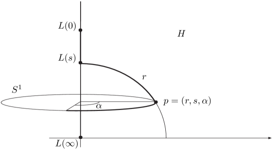
Figure 1. Coordinates for the Riemannian manifold $M$

Let $g(r,s):=\sinh^{2}(r)$ for $r<{1}/{10}$ (the complete definition is given below), then the above metric smoothly extends to the whole manifold $M$, where $M$ is now rotationally symmetric with respect to the axis $L$ and for $r<{1}/{10}$ isometric to the three dimensional hyperbolic space $\mathbb{H}^{3}$ with constant sectional curvature $-1$, cf. [6]. From that it is clear that the Riemannian manifold $(M,g)$ is complete.

2.1. Computation of the sectional curvature

From now on we fix the basis

$$\partial_{1}:=\frac{\partial}{\partial r},\ \partial_{2}:=\frac{\partial}{\partial s},\ \partial_{3}:=\frac{\partial}{\partial\alpha}$$

for the tangent space $T_{p}M$ in $p\in M$. Herein the Christoffel symbols of the Levi-Civita connection can be computed as follows – the indices refer to the corresponding tangent vectors of the basis:

$$\Gamma^{1}_{22} =-\frac{1}{2}h^{\prime}_{r}, \qquad\Gamma^{2}_{12} =\Gamma^{2}_{21}=\frac{h^{\prime}_{r}}{2h}, \qquad\Gamma^{3}_{13} =\Gamma^{3}_{31}=\frac{g^{\prime}_{r}}{2g},$$

$$\Gamma^{1}_{33} =-\frac{1}{2}g^{\prime}_{r}, \qquad\Gamma^{2}_{33} =-\frac{g^{\prime}_{s}}{2h}, \qquad\Gamma^{3}_{23} =\Gamma^{3}_{32}=\frac{g^{\prime}_{s}}{2g},$$

all others equal $0$. Herein $g^{\prime}_{r}$ denotes the partial derivative of the function $g$ with respect to the variable r, $g^{\prime}_{s}$ the partial derivative with respect to $s$, etc.
For the computation of the sectional curvatures $\mathop{\mathchoice{\text{\rm Sect}}{\text{\rm Sect}}{\text{\rm Sect}}{\text{\rm Sect}}}\nolimits^{M}$ write $X=(x_{1},x_{2},x_{3})$ and $Y=(y_{1},y_{2},y_{3})$ for tangent vectors $X,Y\in T_{p}M$ in terms of the basis $\partial_{1},\partial_{2},\partial_{3}$. Then one gets

$$\begin{split}\langle R(X,Y)Y,X\rangle&=\underbrace{\left(-\frac{1}{2}h^{\prime\prime}_{rr}+\frac{1}{4}\frac{(h^{\prime}_{r})^{2}}{h}\right)}_{=:A}(x_{1}y_{2}-x_{2}y_{1})^{2}\\ &+\underbrace{\left(-\frac{1}{2}g^{\prime\prime}_{rr}+\frac{1}{4}\frac{(g^{\prime}_{r})^{2}}{g}\right)}_{=:B}(x_{1}y_{3}-x_{3}y_{1})^{2}\\ &+\underbrace{\left(-\frac{1}{2}g^{\prime\prime}_{ss}-\frac{1}{4}g^{\prime}_{r}h^{\prime}_{r}+\frac{1}{4}\frac{(g^{\prime}_{s})^{2}}{g}\right)}_{=:C}(x_{2}y_{3}-x_{3}y_{2})^{2}\\ &+2\cdot\underbrace{\left(-\frac{1}{2}g^{\prime\prime}_{rs}+\frac{1}{4}\frac{g^{\prime}_{s}h^{\prime}_{r}}{h}+\frac{1}{4}\frac{g^{\prime}_{r}g^{\prime}_{s}}{g}\right)}_{=:D}(x_{1}y_{3}-x_{3}y_{1})(x_{2}y_{3}-x_{3}y_{2}).\end{split}$$

as well as

$$\|X\land Y\|^{2}=h(x_{1}y_{2}-x_{2}y_{1})^{2}+g(x_{1}y_{3}-x_{3}y_{1})^{2}+gh(x_{2}y_{3}-x_{3}y_{2})^{2}.$$

We conclude that the manifold $M$ has strictly negative sectional curvature, i.e.

$$-k^{2}\geq\mathop{\mathchoice{\text{\rm Sect}}{\text{\rm Sect}}{\text{\rm Sect}}{\text{\rm Sect}}}\nolimits^{M}(\text{span}\{X,Y\})=\frac{\langle R(X,Y)Y,X\rangle}{\|X\land Y\|^{2}}$$

for some $k>0$, all $X,Y\in T_{p}M$ and all $p\in M$, if and only if the following inequalities hold:

(2.2) $$\frac{1}{2}h^{\prime\prime}_{rr}-\frac{1}{4}\frac{(h^{\prime}_{r})^{2}}{h} \geq k^{2}h,$$

(2.3) $$\!\!\!\frac{1}{2}g^{\prime\prime}_{rr}-\frac{1}{4}\frac{(g^{\prime}_{r})^{2}}{g} \geq k^{2}g,$$

(2.4) $$\frac{1}{2}g^{\prime\prime}_{ss}+\frac{1}{4}g^{\prime}_{r}h^{\prime}_{r}-\frac{1}{4}\frac{(g^{\prime}_{s})^{2}}{g} \geq k^{2}gh,$$

$$\frac{1}{g^{2}h}\left(-\frac{1}{2}g^{\prime\prime}_{rs}+\frac{1}{4}\frac{g^{\prime}_{s}h^{\prime}_{r}}{h}+\frac{1}{4}\frac{g^{\prime}_{s}g^{\prime}_{r}}{g}\right)^{2} \leq\left(\frac{g^{\prime\prime}_{rr}}{2g}-\frac{(g^{\prime}_{r})^{2}}{4g^{2}}-k^{2}\right)$$

(2.5) $$\qquad\times\left(\frac{g^{\prime\prime}_{ss}}{2gh}+\frac{g^{\prime}_{r}h^{\prime}_{r}}{4gh}-\frac{(g^{\prime}_{s})^{2}}{4g^{2}h}-k^{2}\right).$$

This is explained by the fact that the quadratic form

$$q(X,Y,Z):=(A+k^{2}h)X^{2}+(B+k^{2}g)Y^{2}+(C+k^{2}gh)Z^{2}+2DYZ$$

is non-positive for all $X,Y,Z\in\mathbb{R}$ if and only if

$$-A\geq k^{2}h\,\,\,\text{and}\,\,\,-B\geq k^{2}g\,\,\,\text{and}\,\,\,-C\geq k^{2}gh\,\,\,\text{and}\,\,\,D^{2}\leq(B+k^{2}g)(C+k^{2}gh).$$

2.2. The sphere at infinity $S_{\infty}(M)$

As it is obvious that, for $(s,\alpha)\in\mathbb{R}\times{[\,0,2\pi[}$ fixed, the curves

$$\gamma_{s\alpha}\colon\mathbb{R}_{+}\to M,\quad r\mapsto(r,s,\alpha)$$

form a foliation of $M$ by geodesic rays, we can describe the sphere at infinity $S_{\infty}(M)$ as the union of the “endpoints” (i.e. equivalence classes) $\gamma_{s\alpha}(+\infty)$ of all geodesic rays $\gamma_{s\alpha}$ foliating $M$ together with the equivalence classes $L(+\infty)$ and $L(-\infty)$ determined by the geodesic axis $L$ of $M$, which sums up to:

$$S_{\infty}(M)=L(+\infty)\cup\big{\{}\gamma_{s\alpha}(+\infty)\,|\,(s,\alpha)\in\mathbb{R}\times{[\,0,2\pi[}\big{\}}\cup L(-\infty).$$

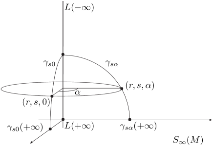
Figure 2. Sphere at Infinity $S_{\infty}(M)$

This also explains why it suffices to show that the $s$-component $S_{t}$ of the Brownian motion $X_{t}$ converges to $+\infty$ as $t$ approaches the lifetime $\zeta$ of the Brownian motion, if we want to show that $X_{t}$ converges for $t\to\zeta$ to the single point $L(+\infty)$ on the sphere $S_{\infty}(M)$ at infinity.

2.3. Properties of the function $g$

We give a brief description of the properties which the warped product function $g\colon\mathbb{R}_{+}\times\mathbb{R}\to\mathbb{R}_{+}$ in (2.1) has to satisfy to provide an example of a Riemannian manifold where the Dirichlet problem at infinity is not solvable whereas there exist non-trivial bounded harmonic functions. We give the idea how to construct such a function $g$ and refer to Borbély [6] for further details.

Lemma 2.1.

There is a ${C}^{\infty}$-function $g\colon\mathbb{R}_{+}\times\mathbb{R}\to\mathbb{R}_{+}$, $(r,s)\mapsto g(r,s)$ satisfying the following properties:

1. $g^{\prime}_{r}\geq 0$ and $g^{\prime}_{s}\geq 0$.

2. $g(r,s)=\sinh^{2}(r)$ for $r<1/{10}$, and for $r\geq 1/{10}$ it holds that:

   $$g^{\prime}_{r}\geq h^{\prime}_{r}g\;\;\text{ and }\;\;\frac{1}{2}g^{\prime\prime}_{rr}-\frac{1}{4}\frac{(g^{\prime}_{r})^{2}}{g}\geq\frac{h^{\prime}_{r}g^{\prime}_{r}}{8}.$$

3. Denoting $p(r,s):={g^{\prime}_{s}}/({g^{\prime}_{r}h})$ one has $(ph)^{\prime}_{s}\geq 0$ and for all $s\in\mathbb{R}$:

   $$\int_{0}^{\infty}p(r,s)\,dr=\infty.$$

4. The function $p(r,s)$ satisfies:

   $$p\leq\frac{1}{1000},\ \,p^{\prime}_{s}\leq\frac{1}{1000},\ |\,p^{\prime}_{r}\,|\leq\frac{5}{1000}\ \text{ and }\ pp^{\prime}_{r}h^{2}<\frac{h^{\prime}_{r}}{1000}.$$

5. We further need that

   $$(ph)^{\prime}_{r}\geq 0,\quad(ph)^{\prime\prime}_{rr}\geq 0$$

   and that there exists $\varepsilon\in{]0,1/4[}$ such that

   (2.6) $$(ph)^{\prime\prime}_{rr}(r)\geq\frac{\varepsilon}{p(r,0)h(r)}\ \ \text{for all}\ \ r\geq 2.$$

6. The function $p(r,s)$ finally has to fulfill:

   $$\int_{r_{0}}^{\infty}\frac{1}{p(r,s)h(r)}\,dr=\infty$$

   for every $r_{0}>0$ and every $s\in\mathbb{R}$.

The following remark summerizes briefly the significance of these conditions.

Remark 2.2 (Comments on the properties listed above).

1. As mentioned in the definition of the Riemannian metric on $M$, property (2) assures that the Riemannian metric smoothly extends to the geodesic $L$ and that curvature condition (2.3) is satisfied for a suitable $k$.

2. The conditions in (4) stated for $p(r,s)$ assure validity of the curvature condition (2.5) – at least for $k=1/{1000}$.

3. The integral condition (3) forces Brownian motion $X=(R,S,A)$ on $M$ to converge to the single point $L(\infty)\in S_{\infty}(M)$ as $t\to\zeta$ which as an immediate consequence implies non-solvability of the Dirichlet problem at infinity for $M$. The given condition assures that the drift term in the stochastic differential equation for the component $S$ of the Brownian motion $X$ compared with the drift term appearing in the defining equation for the component $R$ grows “fast enough” to ensure $S_{t}$ going to $\infty$ as $t$ approaches the lifetime of the Brownian motion.

   In [6], Lemma 2.1, Borbély uses this condition to show that the convex hull of any neighbourhood of $L(\infty)$ is the whole manifold $M$. This is a natural first step in the construction of a manifold for which the Dirichlet problem at infinity is not solvable (cf. the Introduction and [7], [6]).

4. Property (6) is needed for the Brownian motion to almost surely enter a region where $S_{t}$ has nonzero and positive drift (see the construction of $\ell$ and ${\mathscr{D}}$ below); otherwise $S_{t}$ might converge in $\mathbb{R}$ with a positive probability.

2.4. Construction of the function $g$

The idea to construct a function $g$ with the wanted properties is as follows. As $g$ is given as solution of the partial differential equation

(2.7) $$g^{\prime}_{s}(r,s)=p(r,s)h(r)g^{\prime}_{r}(r,s)$$

one has to find an appropriate function $p(r,s)$ and the required initial conditions for $g$ to obtain the desired function.

We will see later that the construction of the metric on $M$ is similar to that given in Ancona [2], as Borbély also defines the function $p$ “stripe-wise” to control the requirements for $p$, $g$ respectively, on each region of the form $[r_{i},r_{j}]\times\mathbb{R}$. Yet he is mainly concerned with the definition of the “drift ratio” $p$, what makes it harder to track the behaviour of the metric function $g$ and to possibly modify his construction for other situations, whereas Ancona gives a more or less direct way to construct the coupling function in the warped product. As a consequence this allows to extend his example to higher dimensions and to adapt it to other situations as well.

We start with a brief description how to construct the function

$$p_{0}(r):=p(r,0),$$

as given in [6]: $p_{0}$ is defined inductively on intervals $[r_{n},r_{n+1}]$, where $r_{n+1}-r_{n}>3$ and $r_{1}>3$ sufficiently large, see below. We let $p_{0}:=0$ on $[0,2]$ and define it on $[2,3]$ as a slowly increasing function satisfying conditions (4) and (5). For $r\in[3,r_{1}]$ let $p_{0}(r):=p_{0}(3)$ be constant, where $r_{1}$ is chosen big enough such that $(p_{0}h)(r_{1})>1$ and $r_{1}/h(r_{1})<1/{1000}$. On the interval $[r_{1},\infty[$ we choose the function $p_{0}$ to be decreasing with $\lim_{r\to\infty}p_{0}(r)=0$, whereas $p_{0}h$ is still increasing and strictly convex; see [6], Lemma 2.3 and Lemma 2.4.

On the interval $[r_{1},r_{2}]$ for $r_{2}$ big enough as given below (and in general on intervals of the form $[r_{2n-1},r_{2n}]$) one extends $p_{0}h$ via a solution of the differential equation

$$y^{\prime\prime}={1}/{(2y)}.$$

Note that carefully smoothing the function $p_{0}$ on the interval $[r_{1},r_{1}+1]$ (and on $[r_{2n-1},r_{2n-1}+1]$ respectively) to become ${C}^{\infty}$ does not interfere with the properties (4) and (5) of $p_{0}$ and can be done such that $(p_{0}h)^{\prime\prime}>1/{(4p_{0}h)}$ is still valid.

Lemma 2.4 in [6] shows that in fact $p_{0}\equiv{p_{0}h}/{h}$ decreases on $[r_{2n-1},r_{2n}]$ and again by [6], Lemma 2.3, for given $r_{2n-1}$ one can choose the upper interval bound $r_{2n}$ such that

$$\int_{r_{2n-1}}^{r_{2n}}\frac{1}{p_{0}h}\,dr>1\quad\text{ for all }n,$$

which guarantees property (6) for $p_{0}$.

On the interval $[r_{2},r_{3}]$ with $r_{3}$ sufficiently large as given below and in general on intervals of the form $[r_{2n},r_{2n+1}]$, let $p_{0}={c_{n}}/{r}$ for some well chosen constant $c_{n}$. This differs from the construction of [6] p. 228 where $p_{0}$ is chosen to be constant in these intervals, but it does not change the properties of the manifold. As above, smoothing on intervals $[r_{2n}-1,r_{2n}]$ preserves the conditions (4), (5) and $(p_{0}h)^{\prime\prime}>\varepsilon/{(p_{0}h)}$ for $0<\varepsilon<1/4$ small enough and independent of $n$, but depending on the choice of $p_{0}$ on ${[2,3[}$.

If one chooses for given $r_{2}$, $r_{2n}$ respectively, the interval bounds $r_{3}$, $r_{2n+1}$ respectively, large enough we can achieve that

$$\int_{r_{2n}}^{r_{2n+1}}p_{0}(r)\,dr>1\quad\text{ for all }n,$$

which finally assures property (3) for $p_{0}$.

Following Borbély [6], one defines $p(r,s)$ via $p_{0}(r)$ as

$$p(r,s):=\chi(r,s)p_{0}(r)$$

by using a “cut-off function” $\chi(r,s)$. Herein $\chi(r,s)$ is given as $\chi(r,s):=\xi(s+\ell(r))$, where $\xi$ is smooth and increasing with $\xi(y)=0$ for $y<0$, $\xi(y)=1/2$ for $y>4$ and $\xi^{\prime},|\xi^{\prime\prime}|<1/2$, $\xi^{\prime\prime}+\xi>0$. The function $\ell$ satisfies $\ell(0)=0$, $\ell^{\prime}(r)=0$ on the interval $[0,2]$ and $\ell^{\prime}(r)={\varepsilon}/(p_{0}h)(r)$ on the interval $[3,\infty[$, with the same $\varepsilon$ as in (2.6). Then the two pieces are connected smoothly such that for $r>0$

(2.8) $$\ell^{\prime\prime}(r)\geq-\varepsilon\frac{(p_{0}h)^{\prime}_{r}(r)}{p_{0}h(r)}\quad\hbox{and}\quad 0\leq\ell^{\prime}\leq\frac{\varepsilon}{p_{0}h}.$$

The function $\ell$ is nondecreasing such that $\lim_{r\to\infty}\ell(r)=\infty$ (see (6) in Lemma 2.1), and one can check that $p(r,s)$ satisfies the required properties listed in Lemma 2.1 (see [6], p. 228ff).

For an appropriate initial condition to solve the partial differential equation (2.7), we set $\widetilde{g_{0}}(r):=\sinh^{2}(r)$ on $[0,\frac{1}{10}]$. On $[\frac{1}{10},\infty[$ let $\widetilde{g_{0}}(r)$ be the solution of the differential equation

$$f^{\prime}=\frac{1}{\sinh^{2}\left(1/{10}\right)}\,h^{\prime}_{r}f\,\,\text{ with initial condition }f\left(\frac{1}{10}\right)=\sinh^{2}\left(\frac{1}{10}\right).$$

Smoothing $\widetilde{g_{0}}$ yields a ${C}^{\infty}$-function $g_{0}$ such that $\widetilde{g_{0}}=g_{0}$ on ${[0,\frac{1}{10}-\delta]}\cup{[\frac{1}{10}+\delta,\infty[}$ for an appropriate $\delta$. In particular, there exist $d_{1},\,d_{2}>0$ such that

(2.9) $$g_{0}(r)=d_{2}e^{d_{1}\sinh^{2}r}\quad\hbox{for all}\quad r\geq\frac{1}{10}+\delta.$$

The function $g_{0}$ serves as initial condition to solve the partial differential equation

$$g^{\prime}_{s}(r,s)=p(r,s)h(r)g^{\prime}_{r}(r,s).$$

Figure 3. Graph of $s\mapsto\gamma(r_{0},s_{0},s)$

More precisely, it is proven in [6] that all trajectories of the vector field $-Z:=-(ph)\frac{\partial}{\partial r}+\frac{\partial}{\partial s}$ intersect the domain

$${\mathscr{D}}:=\left\{(s,r)\in\mathbb{R}\times\mathbb{R}_{+},\ s<-\ell(r)\right\}.$$

Letting $s\mapsto(\gamma(r_{0},s_{0},s),s)$ be the integral curve of $-Z$ satisfying $\gamma(r_{0},s_{0},s_{0})=r_{0}$, we define $f(r_{0},s_{0})$ by

(2.10) $$f(r_{0},s_{0})=\gamma(r_{0},s_{0},-\ell(f(r_{0},s_{0}))).$$

Then (see Sect. 5 for details)

(2.11) $$g(r_{0},s_{0})=g_{0}(f(r_{0},s_{0})).$$

3. Asymptotic behaviour of Brownian motion on $M$

Let $(\Omega;{\mathscr{F}};\mathbb{P})$ be a filtered probability space satisfying the usual conditions and $X$ a Brownian motion on $M$ considered as a diffusion process with generator $\frac{1}{2}\Delta_{M}$ taking values in the Alexandroff compactification $\widetilde{M}:=M\cup\{\infty\}$ of $M$. Further let $\zeta$ denote the lifetime of $X$, i.e. $X_{t}(\omega)=\infty$ for $t\geq\zeta(\omega)$, if $\zeta(\omega)<\infty$.

As we have fixed the coordinate system

$$M=\big{\{}(r,s,\alpha):r\in\mathbb{R}_{+},\ s\in\mathbb{R},\ \alpha\in{[0,2\pi[}\big{\}}$$

for our manifold $M$, we consider the Brownian motion $X$ in the chosen coordinates as well and denote by $(R_{t})_{t<\zeta}$, $(S_{t})_{t<\zeta}$ and $(A_{t})_{t<\zeta}$ the component processes of $(X_{t})_{t<\zeta}$. The generator $\frac{1}{2}\Delta_{M}$ of $X$ is then written in terms of the basis $\frac{\partial}{\partial r},\frac{\partial}{\partial s},\frac{\partial}{\partial\alpha}$ of $TM$ as:

(3.12) $$\begin{split}\frac{1}{2}\Delta_{M}&=\frac{1}{2}\left(\frac{\partial^{2}}{\partial r^{2}}+\frac{1}{h}\frac{\partial^{2}}{\partial s^{2}}+\frac{1}{g}\frac{\partial^{2}}{\partial\alpha^{2}}\right)+\left(\frac{h^{\prime}_{r}}{4h}+\frac{g^{\prime}_{r}}{4g}\right)\frac{\partial}{\partial r}+\frac{g^{\prime}_{s}}{4gh}\frac{\partial}{\partial s}.\end{split}$$

Therefore we can write down a system of stochastic differential equations for the components $R,S$ and $A$ of our given Brownian motion:

(3.13) $$dR_{t} =\left(\frac{h^{\prime}_{r}(R_{t})}{4h(R_{t})}+\frac{g^{\prime}_{r}(R_{t},S_{t})}{4g(R_{t},S_{t})}\right) dt\,\, + dW^{1}$$

(3.14) $$dS_{t} =\frac{g^{\prime}_{s}(R_{t},S_{t})}{4g(R_{t},S_{t})h(R_{t})} dt\,\, +\quad\;\frac{1}{\sqrt{h(R_{t})}} dW^{2}$$

(3.15) $$dA_{t} =\quad \quad\;\;\frac{1}{\sqrt{g(R_{t},S_{t})}}\,\, dW^{3}$$

with a three-dimensional Euclidean Brownian motion $W=(W^{1},W^{2},W^{3})$.

As already mentioned, we are going to read the component $A$ of the Brownian motion with values in the universal covering $\mathbb{R}$ of $S^{1}$.

Remark 3.1.

Inspecting the defining stochastic differential equations for the components $R$, $S$ and $A$ of the Brownian motion $X$ on $M$, it is interesting to note that the behaviour of the component $A_{t}$ does not influence the behaviour of the components $R_{t}$ and $S_{t}$. The first two equations can be solved independently of the third one; their solution then defines the third component of the Brownian motion. Hence it is clear that the lifetime $\zeta$ of $X_{t}$ does not depend on the component $A_{t}$ – in particular does not depend on the starting point $A_{0}$ of $A_{t}$. We are going to use this fact later to prove existence of non-trivial bounded harmonic functions on $M$.

As we we are going to see in Section 4.3 the “drift ratio” $p(r,s)={g^{\prime}_{s}}/({g^{\prime}_{r}h})$ influences the interplay of the components $S_{t}$ and $R_{t}$ of the Brownian motion and therefore determines the behaviour of the Brownian paths. For this reason it is more convenient to work with a time-changed version $\widetilde{X}_{t}$ of our Brownian motion, where the drift of the component $\widetilde{R}_{t}$ is just $t$ and the drift of $\widetilde{S}_{t}$ is essentially given by $p$. This can be realized with a time change $(\tau_{t})$ defined as follows:

Let

$$T(t):=\int_{0}^{t}\left(\frac{h^{\prime}_{r}}{4h}+\frac{g^{\prime}_{r}}{4g}\right)(S_{u},R_{u})\,du$$

and $\tau_{t}:=T^{-1}(t)\equiv\inf\{s\in\mathbb{R}_{+}:T(s)\geq t\}$ for $t\leq T(\zeta)$. The components $\widetilde{R}_{t},\widetilde{S}_{t},\widetilde{A}_{t}$ of the time-changed Brownian motion $\widetilde{X}_{t}:=X_{\tau_{t}}$ are then given for $t\leq\widetilde{\zeta}:=T(\zeta)$ by the following system of stochastic differential equations:

(3.16) $$d\widetilde{R}_{t} = dt\,\, + \frac{1}{\sqrt{\frac{h^{\prime}_{r}}{4h}(\widetilde{R}_{t})+\frac{g^{\prime}_{r}}{4g}(\widetilde{R}_{t},\widetilde{S}_{t})}}\,\, dW^{1}$$

(3.17) $$d\widetilde{S}_{t} =\frac{g^{\prime}_{s}(\widetilde{R}_{t},\widetilde{S}_{t})}{(gh^{\prime}_{r}+g^{\prime}_{r}h)(\widetilde{R}_{t},\widetilde{S}_{t})}\,\,\, dt\,\, + \frac{1}{\sqrt{h(\widetilde{R}_{t})\left(\frac{h^{\prime}_{r}}{4h}(\widetilde{R}_{t})+\frac{g^{\prime}_{r}}{4g}(\widetilde{R}_{t},\widetilde{S}_{t})\right)}}\,\, dW^{2}$$

(3.18) $$d\widetilde{A}_{t} = \frac{1}{\sqrt{g(\widetilde{R}_{t},\widetilde{S}_{t})\left(\frac{h^{\prime}_{r}}{4h}(\widetilde{R}_{t})+\frac{g^{\prime}_{r}}{4g}(\widetilde{R}_{t},\widetilde{S}_{t})\right)}}\,\, dW^{3}.$$

We are now going to state the main theorem of this chapter which shows that from the stochastic point of view the Riemannian manifold $(M,\gamma)$ constructed by Borbély [6] has essentially the same properties as the manifold of Ancona in [2]. We further give a stochastic construction of non-trivial bounded harmonic functions on $M$, which is more transparent than the existence proof of Borbély relying on Perron’s principle.

Theorem 3.2 (Behaviour of Brownian motion on $M$).

1. For the Brownian motion $X$ on the Riemannian manifold $(M,\gamma)$ constructed above the following statement almost surely holds:

   $$\lim_{t\to\zeta}X_{t}=L(+\infty),$$

   independently of the starting point $X_{0}$. In particular the Dirichlet problem at infinity for $M$ is not solvable.

2. The component $A_{t}$ of Brownian motion $X_{t}$ almost surely converges to a random variable $A_{\zeta}$ which possesses a positive density on $S^{1}$.

3. The lifetime $\zeta$ of the process $X$ is a.s. finite.

Proof.

From Eqs. (3.16),  (3.17) and  (3.18) we immediately see that the derivatives of the brackets of $\widetilde{R}$ and $\widetilde{S}$ are bounded, and that the drift of $\tilde{S}$ takes its values in $[0,\max p]$ and is therefore bounded. As a consequence the process $(\widetilde{R},\widetilde{S},\widetilde{A})$ has infinite lifetime.

Moreover for all $\beta>0$, we have almost surely $|R_{t}-t|\leq\beta t$ eventually. From this and the fact that ${g_{r}^{\prime}}/{g}\geq h_{r}^{\prime}$ for $r\geq{1}/{10}$ we deduce that the martingale parts of $\widetilde{R}$ and $\widetilde{S}$ together with the process $\widetilde{A}$ converge as $t$ tends to infinity.

Next we see from

$$\frac{g_{s}^{\prime}}{gh_{r}^{\prime}+g_{r}^{\prime}h}=\frac{phg_{r}^{\prime}}{gh_{r}^{\prime}+g_{r}^{\prime}h}\leq p$$

that for $t$ sufficiently large the drift of $\widetilde{S}$ is larger that $p_{0}((1+\beta)t)/2$. Consequently $\widetilde{S}$ tends to infinity as $t\to\infty$. To prove (1) it is sufficient to establish

$$\lim_{t\to\infty}\widetilde{X}_{t}=L(+\infty)$$

and this is a consequence of the fact that $\widetilde{S}_{t}$ converges to infinity. The proof of (2) is a direct consequence of the convergence of $\widetilde{A}_{t}$ to a random variable which conditioned to $\widetilde{R}$ and $\widetilde{S}$ is Gaussian (in $\mathbb{R}$) and non-degenerate. We are left to prove (3). Changing back the time of the process $\widetilde{X}$, we get

(3.19) $$\zeta=\int_{0}^{\infty}\left(\frac{h_{r}^{\prime}}{4h}+\frac{g_{r}^{\prime}}{4g}\right)^{-1}\left(\widetilde{R}_{t},\widetilde{S}_{t}\right)\,dt.$$

But, for large $r$ and $s\geq 0$, we have

$$\left(\frac{h_{r}^{\prime}}{4h}+\frac{g_{r}^{\prime}}{4g}\right)(r,s)\geq\frac{g_{r}^{\prime}}{4g}\geq\frac{1}{2}\cosh r\sinh r.$$

As a.s. $\widetilde{R}_{t}-t\geq-\beta t$ eventually and as $\widetilde{S}_{t}$ converges to infinity as $t$ tends to infinity, we get the result. ∎

4. Non-trivial shift-invariant events

As explained in the Introduction there is a one-to-one correspondence between the $\sigma$-field ${{\mathscr{F}}}_{\operatorname{inv}}$ of shift-invariant events for $X$ up to equivalence and the set of bounded harmonic functions on $M$. We are going to use this fact and give a probabilistic proof for the existence of non-trivial shift-invariant random variables, which in turn yields non-trivial bounded harmonic functions on $M$. In addition, we get a stochastic representation of the constructed harmonic functions as “solutions of a modified Dirichlet problem at infinity”. In contrast to the usual Dirichlet problem at infinity however, the boundary function does not live on the geometric horizon $S_{\infty}(M)\cong S^{d-1}(M)$, and the harmonic functions are not representable in terms of the limiting angle of Brownian motion.

4.1. Shift-invariant variables

In the discussed example it turns out that the shift-invariant random variable $A_{\zeta}$ is non-trivial and can be interpreted as “$1$-dimensional angle” on the sphere $S_{\infty}(M)$ at infinity. The variable $A_{\zeta}$ gives the direction on the horizon, wherefrom the Brownian motion $X$ converges to the limiting point $L(\infty)$. Despite the fact that the limit $X_{\zeta}\in S_{\infty}(M)$ itself is trivial, and hence the limiting angle $\vartheta(X)_{\zeta}\in S^{d-1}(M)$ as well, Brownian paths for large times can be distinguished by their projection onto $S_{\infty}(M)$. Taking into account that in the pinched curvature case the angular part carries all shift-variant information, one might conjecture that the random variable $A_{\zeta}$ already generates the shift-invariant $\sigma$-field ${{\mathscr{F}}}_{\operatorname{inv}}$. In turn this would imply a stochastic representation for bounded harmonic functions $h$ on $M$ as

$$h(x)=\mathbb{E}^{x}[f(A_{\zeta})]=\mathbb{E}^{x}\left[\lim_{t\to\zeta}f(\mathop{\mathchoice{\text{\rm pr}}{\text{\rm pr}}{\text{\rm pr}}{\text{\rm pr}}}\nolimits_{3}(X_{t}))\right]$$

with $f\colon S^{1}\to\mathbb{R}$ measurable. However, Borbély [6] describes a way to construct a family of harmonic functions $\psi(r,s)$ which are rotationally invariant, i.e. independent of $\alpha$, and therefore cannot be of the above form. As he uses “Perron’s principle” for the construction, these harmonic functions do not come with an explicit representation. Put in the probabilistic framework, we learn from this that there must be a way to obtain non-trivial shift-invariant events also in terms of the components $S_{t}$ and $R_{t}$ of the Brownian motion. Indeed, as will be seen in Theorem 4.2, there exists a non-trivial shift-invariant random variable of the form

$$\lim_{t\to\zeta}\left(\widetilde{S}_{t}-\int_{0}^{\widetilde{R}_{t}}q(r)\,dr\right).$$

Herein $\widetilde{S}$ and $\widetilde{R}$ are time-changed versions of $S$ and $R$ and $q\colon\mathbb{R}_{+}\to\mathbb{R}$ is a function already constructed by Borbély, whose properties are listed in Lemma 4.1 below. This finally leads to additional (to that depending on the component $\alpha$) harmonic functions via the stochastic representation

$$h(x)=\mathbb{E}^{x}\left[g\left(\lim_{t\to\zeta}\left(\widetilde{S}_{t}-\int_{0}^{\widetilde{R}_{t}}q(r)\,dr\right)\right)\right],$$

where $g\colon\mathbb{R}\to\mathbb{R}$ is a bounded measurable function.

Lemma 4.1.

There is a ${C}^{\infty}$-function $q\colon\mathbb{R}_{+}\to\mathbb{R}$ with the following properties:

1. $$q(r)=-\frac{\sinh(r)}{\cosh^{2}(r)}=\left(\frac{1}{\sqrt{h}}\right)^{\prime}\text{ for }r\leq T_{1}.$$

2. For $r>T_{1}$ the function $q$ satisfies the inequalities

   $$-3|q|<q^{\prime}<\frac{1}{\cosh(r)},\qquad\qquad\left(\frac{1}{\sqrt{h}}\right)^{\prime}\leq q\leq\frac{p_{0}}{2}-\frac{40}{h}.$$

3. There is a $T_{2}>T_{1}$ such that

   $$q(r)=\frac{p_{0}(r)}{2}-\frac{40}{h(r)}\text{ for }r\geq T_{2}.$$

Proof.

See Section 4.2 below and [6]. ∎

Theorem 4.2.

Consider $\widetilde{Z}_{t}=\widetilde{S}_{t}-\int_{0}^{\widetilde{R}_{t}}q(u)\,du$ as before. The limit variable

$$\widetilde{Z}_{\infty}:=\lim_{t\to\infty}\widetilde{Z}_{t}$$

exists. Moreover the law of the random variable $(\widetilde{Z}_{\infty},\widetilde{A}_{\infty})=(Z_{\zeta},A_{\zeta})$ has full support $\mathbb{R}\times S^{1}$ and is absolutely continuous with respect to the Lebesgue measure.

Proof.

Let $t(r,s)=\log g(r,s)$ and

$$m(r,s)=\frac{2}{\sqrt{({h_{r}^{\prime}}/{h})(r)+t_{r}^{\prime}(r,s)}}.$$

Then a straight-forward calculation shows that

(4.1) $$\begin{split}d\widetilde{Z}_{t}&=\left(-p(\widetilde{R}_{t},\widetilde{S}_{t})\frac{h^{\prime}_{r}}{4h}(\widetilde{R}_{t})m^{2}(\widetilde{R}_{t},\widetilde{S}_{t})-\frac{1}{2}q^{\prime}(\widetilde{R}_{t})m^{2}(\widetilde{R}_{t},\widetilde{S}_{t})\right)\,dt\\ &\qquad+(p(\widetilde{R}_{t},\widetilde{S}_{t})-q(\widetilde{R}_{t}))\,dt-q(\widetilde{R}_{t})m(\widetilde{R}_{t},\widetilde{S}_{t})\,dW_{t}^{1}+\frac{m(\widetilde{R}_{t},\widetilde{S}_{t})}{\sqrt{h(\widetilde{R}_{t})}}\,dW_{t}^{2}.\end{split}$$

When $\widetilde{R}_{t}$ is sufficiently large, this simplifies as

(4.2) $$\begin{split}d\widetilde{Z}_{t}&=\left(-p(\widetilde{R}_{t},\widetilde{S}_{t})\frac{h^{\prime}_{r}}{4h}(\widetilde{R}_{t})m^{2}(\widetilde{R}_{t},\widetilde{S}_{t})-\frac{1}{2}q^{\prime}(\widetilde{R}_{t})m^{2}(\widetilde{R}_{t},\widetilde{S}_{t})+\frac{40}{h(\widetilde{R}_{t})}\right)\,dt\\ &\qquad-q(\widetilde{R}_{t})m(\widetilde{R}_{t},\widetilde{S}_{t})\,dW_{t}^{1}+\frac{m(\widetilde{R}_{t},\widetilde{S}_{t})}{\sqrt{h(\widetilde{R}_{t})}}\,dW_{t}^{2}.\end{split}$$

For $t$ sufficiently large, we know that $|\widetilde{R}_{t}-t|\leq\beta t$ (for any small $\beta$) and that $\widetilde{S}_{t}$ is positive; furthermore $t_{r}^{\prime}$ is larger than $2\cosh r\sinh r$ for $r$ large and $s\geq 0$. This together with the fact that the functions $p$, $({h_{r}^{\prime}}/{4h})$ $q^{\prime}$, $q$ and $1/{\sqrt{h}}$ are bounded allows to conclude that $\widetilde{Z}$ is converging.

To prove that the law of $\widetilde{Z}_{\infty}$ has full support on $\mathbb{R}$, it is sufficient to establish convergence of the finite variation part of $\widetilde{Z}$, and that its diffusion coefficient is eventually bounded below by a continuous positive deterministic function and above by $e^{-\beta t}$ for some $\beta>0$. Indeed, with these properties it is easy to prove that, taking any open non empty interval $I$ of $\mathbb{R}$, there is a time $t$ such that after time $t$, the process $\widetilde{Z}$ will hit the center of $I$ and then stay in $I$ with positive probability.

The convergence of the drift has already been established, together with the upper bound of the diffusion coefficient. To obtain the lower bound, we use Eq. (5.8) of Lemma 5.1 below, along with the fact that eventually ${t}/2\leq\widetilde{R}_{t}\leq 2t$ and $\widetilde{S}_{t}\leq t$, to obtain

$$t_{r}^{\prime}(\widetilde{R}_{t},\widetilde{S}_{t})\leq C_{2}(h\circ f)(2t,t)\,\frac{((p_{0}h)\circ f)(2t,t)}{(p_{0}h)\left(t/2\right)}$$

for some $C_{2}>0$, where $f$ is defined at the end of Sect. 2. This immediately yields a lower bound for the diffusion coefficient $h(\widetilde{R}_{t})^{-1/2}\,m(\widetilde{R}_{t},\widetilde{S}_{t})$ of the form

$$ce^{-2t}\left((h\circ f)(2t,t)\,\frac{((p_{0}h)\circ f)(2t,t)}{(p_{0}h)\left(t/2\right)}\right)^{-1/2}$$

(for some $c>0$) which is a positive continuous function.

The assertion on the support of the law of $(\widetilde{Z}_{\infty},\widetilde{A}_{\infty})$ is then a direct consequence of the fact that conditioned to $(\widetilde{R},\widetilde{Z})$, the random variable $\widetilde{A}_{\infty}$ is a non-degenerate Gaussian variable.

We are left to prove that the law of $(\widetilde{Z}_{\infty},\widetilde{A}_{\infty})$ is absolutely continuous. Using the conditioning argument for $\widetilde{A}_{\infty}$, it is sufficient to prove that the law of $\widetilde{Z}_{\infty}$ is absolutely continuous. To this end we use the estimates in Sect. 5. It is proven there that there exists an increasing sequence of subsets $B_{n}$ of $\Omega$ satisfying $\bigcup_{n\geq 0}B_{n}\mathrel{\mathchoice{\lower 0.5pt\vbox{\halign{$\m@th\displaystyle\hfil#\hfil$\cr\hbox{\sevenrm a.s.}\crcr=\crcr}}}{\lower 0.5pt\vbox{\halign{$\m@th\textstyle\hfil#\hfil$\cr\hbox{\sevenrm a.s.}\crcr=\crcr}}}{\lower 0.5pt\vbox{\halign{$\m@th\scriptstyle\hfil#\hfil$\cr\hbox{\sevenrm a.s.}\crcr=\crcr}}}{\lower 0.5pt\vbox{\halign{$\m@th\scriptscriptstyle\hfil#\hfil$\cr\hbox{\sevenrm a.s.}\crcr=\crcr}}}}\Omega$ such that on $B_{n}$, for each $n\geq 0$, the diffusion process

$$\breve{U}_{u}:=\big{(}\widetilde{R}_{\tan u}-\tan u,\widetilde{Z}_{\tan u}\big{)}$$

has a continuous extension to $u\in[0,\pi/2]$ and that this extension has bounded coefficients with bounded derivatives up to order $2$. Consequently, following [19] Theorem 4.6.5, there exists a $C^{1}$ flow $\breve{\varphi}(u_{1},u_{2},\omega)$ which almost surely realizes a diffeomorphism from ${]{-\tan u_{1}},\infty[}\times\mathbb{R}$ to ${]{-\tan u_{2}},\infty[}\times\mathbb{R}$ if $u_{2}<\pi/2$ and from ${]{-\tan u_{1}},\infty[}\times\mathbb{R}$ to its image in $\mathbb{R}\times\mathbb{R}$ if $u_{2}=\pi/2$ (for the first assertion one uses the fact that Brownian motion has full support).

As a consequence, the density $\breve{p}_{\pi/4}$ of $\breve{U}_{\pi/4}$ (which exists and is positive on ${]{-\tan\pi/4,\infty}[}\times\mathbb{R}$) is transported by the flow to

$$\breve{p}_{\pi/4}\circ\left(\breve{\varphi}(\pi/4,\pi/2,\omega)\right)^{-1}\big{|}\det J\left(\breve{\varphi}(\pi/4,\pi/2,\omega)\right)^{-1}\big{|}$$

where $J\left(\breve{\varphi}(\pi/4,\pi/2,\omega)\right)^{-1}$ is the Jacobian matrix of $\left(\breve{\varphi}(\pi/4,\pi/2,\omega)\right)^{-1}$. Integrating with respect to $\omega$ proves existence of a positive density $\breve{p}_{\pi/2}$ for $\breve{U}_{\pi/2}$:

$$\breve{p}_{\pi/2}=\mathbb{E}\left[\breve{p}_{\pi/4}\circ\left(\breve{\varphi}(\pi/4,\pi/2,{\kern 0.8pt\cdot\kern 0.8pt})\right)^{-1}\big{|}\det J\left(\breve{\varphi}(\pi/4,\pi/2,{\kern 0.8pt\cdot\kern 0.8pt})\right)^{-1}\big{|}\right].$$

Finally projecting onto the second coordinate gives the density of $\widetilde{Z}_{\infty}$, which proves that its law is absolutely continuous. ∎

4.2. Construction of the function $q$

As the explicit construction of $q$ is already done in [6] we just give a short sketch (following Borbély) how to get a function $q$ with the required properties:

Let $a\in\mathbb{R}_{+}$ and $T_{0}$ such that $p_{0}(r)h(r)>240$ and $\sqrt{h(r)}>80$ for $r>T_{0}$. Let further $T_{1}>T_{0}$ such that $p(r,s)=p_{0}(r)/2$ for $r\geq T_{1}$ and $s\geq a-1$. For $r\leq T_{1}$ the function $q$ is defined as

$$q(r):=\left(\frac{1}{\sqrt{h}}\right)^{\prime}=-\frac{\sinh(r)}{\cosh^{2}(r)}.$$

For $r\geq T_{1}$ choose a strictly increasing ${C}^{\infty}$-extension of $-{\sinh(r)}/{\cosh^{2}(r)}$ such that $q(r)>0$ for $r$ large enough and

$$\left(\frac{1}{\sqrt{h}}\right)^{\prime\prime}<q^{\prime}<\frac{1}{\sqrt{h}}.$$

As $p_{0}(r)/2-{40}/{h(r)}>0$ with

$$\lim_{r\to\infty}\left(\frac{1}{2}p_{0}(r)-\frac{40}{h(r)}\right)=0$$

(due to the construction of $p_{0}$, see Sect. 1) there is an $r>T_{1}$ with $q(r)=p_{0}(r)/2-{h(r)/40}$. Let

$$T_{2}:=\inf\left\{r>T_{1}:q(r)=\frac{1}{2}p_{0}(r)-\frac{40}{h(r)}\right\}.$$

For $r\geq T_{2}$ set

$$q(r):=\frac{1}{2}p_{0}(r)-\frac{40}{h(r)}.$$

The desired function $q$ is then a smoothened version of this function.

Borbély shows in [6], p. 232, that the function $q$ obtained this way meets indeed the additionally required properties

$$-3|q|\leq q^{\prime}\leq\frac{1}{\sqrt{h}}\quad\text{and}\quad\left(\frac{1}{\sqrt{h}}\right)\leq q\leq\frac{1}{2}p_{0}-\frac{40}{h}\,.$$

4.3. Interpretation of the asymptotic behaviour of Brownian motion

We conclude this chapter with some explanations how the behaviour of the Brownian paths on $M$ should be interpreted geometrically.

As seen in Sect. 1 and Sect. 4, the random variables

$$\lim_{t\to\zeta}A_{t}\quad\text{and}\quad\lim_{t\to\zeta}\left(S_{t}-\int_{0}^{R_{t}}q(r)\,dr\right)$$

serve as non-trivial shift-invariant random variables for $X$ and hence yield non-trivial shift-invariant events for $X$.

To give a geometric interpretation of the shift-invariant variable

$$\lim_{t\to\infty}\left(\widetilde{S}_{t}-\int_{0}^{\widetilde{R}_{t}}q(r)\,dr\right),$$

we have to investigate again the stochastic differential equations for $\widetilde{S}_{t}$ and $\widetilde{R}_{t}$:

$$d\widetilde{R}_{t} = dt\,\, + \frac{1}{\sqrt{\frac{h^{\prime}_{r}}{4h}+\frac{g^{\prime}_{r}}{4g}}}\,\, dW^{1}_{t}$$

$$d\widetilde{S}_{t} =\frac{g^{\prime}_{s}}{gh^{\prime}_{r}+g^{\prime}_{r}h}\,\,\, dt\,\, + \frac{1}{\sqrt{h\left(\frac{h^{\prime}_{r}}{4h}+\frac{g^{\prime}_{r}}{4g}\right)}}\,\, dW^{2}_{t}.$$

We have seen in Sect. 4 that the local martingale parts

$$M^{1}_{t}=\int_{0}^{t}\left({\frac{h^{\prime}_{r}}{4h}+\frac{g^{\prime}_{r}}{4g}}\right)^{-1/2}dW^{1}\text{ and }M^{2}_{t}=\int_{0}^{t}\left({h\left(\frac{h^{\prime}_{r}}{4h}+\frac{g^{\prime}_{r}}{4g}\right)}\right)^{-1/2}dW^{2}$$

of $\widetilde{R}_{t}$ and $\widetilde{S}_{t}$ converge almost surely as $t\to\widetilde{\zeta}$. This suggests that the component $\widetilde{R}_{t}$, when observed at times $t$ near $\infty$ (or when starting $X$ near $L(\infty)$), should behave like the solution $r(t):=r_{0}+t$ of the deterministic differential equation

$$\dot{r}=1.$$

From the stochastic differential equation above we get

$$\widetilde{S}_{t}=S_{0}+\int_{0}^{t}\frac{g^{\prime}_{s}(\widetilde{R}_{t},\widetilde{S}_{t})}{g(\widetilde{R}_{t},\widetilde{S}_{t})h^{\prime}_{r}(\widetilde{R}_{t})+h(\widetilde{R}_{t})g^{\prime}_{r}(\widetilde{R}_{t},\widetilde{S}_{t})}\,ds+M^{2}_{t},$$

where the local martingale $M^{2}_{t}$ converges as $t\to\infty$, and $\widetilde{R}_{t}$ is expected to behave like $r_{0}+t$, when the starting point $(r_{0},s_{0},\alpha_{0})$ of $X$ is close to $L(\infty)$. One might therefore expect $\widetilde{S}_{t}$ to behave (for $t$ near to $\infty$) like the solution $s(t)$, starting in $s_{0}$, of the deterministic differential equation

(4.3) $$\dot{s}=\frac{g^{\prime}_{s}(r(t),s)}{g(r(t),s)h^{\prime}_{r}(r(t))+h(r(t))g^{\prime}_{r}(r(t),s)}.$$

It remains to make rigorous the meaning of “should behave like”.

Considering the solutions $r(t),s(t)$ of the deterministic differential equations above, we note that $\Gamma_{s_{0}}\colon\mathbb{R}_{+}\to\mathbb{R}_{+}\times\mathbb{R}$ given as $\Gamma_{s_{0}}(t):=(t,s(t))$ with $\Gamma_{s_{0}}(0)=(0,s_{0})$ is the trajectory of the “drift” vector field

(4.4) $$V_{d}=\frac{\partial}{\partial r}+\frac{g^{\prime}_{s}}{gh^{\prime}_{r}+hg^{\prime}_{r}}\frac{\partial}{\partial s}$$

starting in $(0,s_{0})=L(s_{0})$.

As we are going to see below (see Remark 4.3), the “endpoint”

$$\Gamma_{s_{0}}(+\infty)\equiv\lim_{t\to\infty}\Gamma_{s_{0}}(t)$$

of all the trajectories is just $L(\infty)\in S_{\infty}(M)$. Furthermore, for every point $(r,s)\in\mathbb{R}_{+}\times\mathbb{R}$, there is exactly one trajectory $\Gamma_{s_{0}}$ of $V_{d}$ with $\Gamma_{s_{0}}(r)=(r,s)$, in other words, the union

$$\bigcup_{s_{0}\in\mathbb{R}}\Gamma_{s_{0}}$$

defines a foliation of $H$. Recall that $H$ is one component of $\mathbb{H}\setminus L$ and $M=(H\cup L)\times_{g}S^{1}$. Defining a coordinate transformation

(4.5) $$\begin{split}\Phi\colon\mathbb{R}_{+}\times\mathbb{R}&\to\mathbb{R}_{+}\times\mathbb{R}\\ (r,s)&\mapsto(r,s_{0})\equiv(\Phi_{r}(r,s),\Phi_{s}(r,s)),\end{split}$$

where $s_{0}$ is the starting point of the unique trajectory $\Gamma_{s_{0}}$ with $\Gamma_{s_{0}}(r)=(r,s)$, we obtain coordinates for $\mathbb{R}_{+}\times\mathbb{R}$ where the trajectories $\Gamma_{s_{0}}$ of $V_{d}$ are horizontal lines.

Applying the coordinate transformation $\Phi$ to the components $\widetilde{R}_{t}$ and $\widetilde{S}_{t}$ of the Brownian motion,

$$\Phi(\widetilde{R}_{t},\widetilde{S}_{t})=(\Phi_{r}(\widetilde{R}_{t},\widetilde{S}_{t}),\Phi_{s}(\widetilde{R}_{t},\widetilde{S}_{t})),$$

we are able to compare the behaviour of the components $\widetilde{R}_{t}$ and $\widetilde{S}_{t}$ with the trajectories $\Gamma_{s_{0}}$ of $V_{d}$, in other words, with the deterministic solutions $r(t)$ and $s(t)$. The component $\Phi_{r}(\widetilde{R}_{t},\widetilde{S}_{t})$ obviously equals $\widetilde{R}_{t}$. Yet, knowing that for $t\to\infty$ the new component $\Phi_{s}(\widetilde{R}_{t},\widetilde{S}_{t})$ possesses a non-trivial limit, would mean that the Brownian paths (their projection onto $(H\cup L)$, to be precise) finally approach the point $L(\infty)\in S_{\infty}(M)$ along a (limiting) trajectory $\Gamma_{s_{0}}$, where $s_{0}=\lim_{t\to\infty}\Phi_{s}(\widetilde{R}_{t},\widetilde{S}_{t})$. This would contribute another piece of non-trivial information to the asymptotic behaviour of Brownian motion, namely along which trajectory (or more precisely, along which surface of rotation $\Gamma_{s_{0}}\times S^{1}$) a Brownian path finally exits the manifold $M$.

It remains to verify that the above defined component $\Phi_{s}(\widetilde{R}_{t},\widetilde{S}_{t})$ indeed has a non-trivial limit as $t\to\infty$. As already seen, $\Phi_{s}(\widetilde{R}_{t},\widetilde{S}_{t})$ is the starting point of the deterministic curve $s(t)$, satisfying the differential equation (4.3) with $s(\widetilde{R}_{t})=\widetilde{S}_{t}$. The solution $s(t)$ is of the form

$$s(t)=s_{0}+\int_{0}^{t}f(r(u),s(u))\,du$$

where $f={g^{\prime}_{s}}/{(gh^{\prime}_{r}+hg^{\prime}_{r})}$. In particular, $s(t)$ explicitly depends on $s(u)$ for $u\leq t$. That is the reason why, when applying Itô’s formula to $\Phi_{s}(\widetilde{R}_{t},\widetilde{S}_{t})$, there appear first order derivatives of the flow

$$\Psi\colon\mathbb{R}_{+}\times\mathbb{R}\to\mathbb{R}_{+}\times\mathbb{R},\quad\quad(r,s)\mapsto\Gamma_{s}(r)$$

with respect to the variable $s$. Estimating these terms does not seem to be trivial, nor to provide good estimates in order to establish convergence of $\Phi_{s}(\widetilde{R}_{t},\widetilde{S}_{t})$ as $t\to\infty$.

A possibility to circumvent this problem is to find a vector field $V$ on $T(\mathbb{R}_{+}\times\mathbb{R})$ of the form $\partial/\partial r+f(r)\partial/\partial s$ whose trajectories also foliate $H$ and are not “far off” the trajectories $\Gamma_{s_{0}}$ of $V_{d}$ – in particular the trajectories of $V$ have to exit $M$ through the point $L(\infty)\in S_{\infty}(M)$ as well.

As seen in Sect. 4, we have

$$\left|\,\frac{g^{\prime}_{s}}{gh^{\prime}_{r}+hg^{\prime}_{r}}-p\,\right|\leq\left|\,p\cdot\frac{1}{1+h}\,\right|.$$

Furthermore, for $r\geq T_{2}$ the function $q(r)$ is defined as $p_{0}/2-{40}/{h}$, in particular $q(r)$ does not differ much from the function $p(r,s)$ which equals $p_{0}/2$ for $r$ and $s$ large. Hence $q(r)$ is a good approximation for $g_{s}/(gh^{\prime}_{r}+hg^{\prime}_{r})$ for $r$ large, and is independent of the variable $s$.

We therefore consider the vector field

(4.6) $$V:=\frac{\partial}{\partial r}+q(r)\frac{\partial}{\partial s}.$$

Starting in $(0,s_{0})\in\mathbb{R}_{+}\times\mathbb{R}$ the trajectories $C_{s_{0}}$ of $V$ have the form

$$C_{s_{0}}(t)=\left(t,s_{0}+\int_{0}^{t}q(u)\,du\right).$$

As we are going to see below, we also have $\lim_{t\to\infty}C_{s_{0}}(t)=L(\infty)$, see Remark 4.3, and the union

$$\bigcup_{s_{0}\in\mathbb{R}}C_{s_{0}}$$

forms a foliation of $H$.

For $(r,s)\in\mathbb{R}_{+}\times\mathbb{R}$ there is exactly one trajectory $C_{s_{0}}$ of $V$ with $C_{s_{0}}(r)=s$. Its starting point $s_{0}$ can be computed as $s_{0}=s-\int_{0}^{r}q(u)\,du$. We can therefore define a coordinate transformation

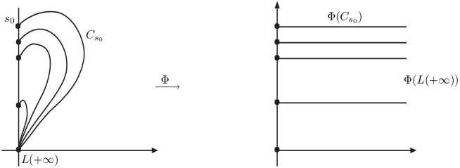
Figure 4. Effect of the coordinate transformation $\Phi$

(4.7) $$\begin{split}\Phi\colon\mathbb{R}_{+}\times\mathbb{R}&\to\mathbb{R}_{+}\times\mathbb{R},\\ (r,s)&\mapsto\left(r,s-\int_{0}^{r}q(u)\,du\right).\end{split}$$

As seen in Figure 4, the trajectories $C_{s_{0}}$ of $V$ are horizontal lines in the new coordinate system.

In the changed coordinate system the components $\widetilde{R}_{t}$ and $\widetilde{S}_{t}$ of $X$ then look like

(4.8) $$\Phi(\widetilde{R}_{t},\widetilde{S}_{t})=\left(\widetilde{R}_{t},\widetilde{S}_{t}-\int_{0}^{\widetilde{R}_{t}}q(u)\,du\right)\equiv\big{(}\Phi_{r}(\widetilde{R}_{t},\widetilde{S}_{t}),\Phi_{s}(\widetilde{R}_{t},\widetilde{S}_{t})\big{)}.$$

As we have proven in Sect. 4,

$$\lim_{t\to\widetilde{\zeta}}\left[\widetilde{S}_{t}-\int_{0}^{\widetilde{R}_{t}}q(u)\,du\right]\equiv\lim_{t\to\widetilde{\zeta}}\Phi_{s}(\widetilde{R}_{t},\widetilde{S}_{t})$$

exists and is a non-trivial shift-invariant random variable. Therefore the non-triviality of $\lim_{t\to\infty}\Phi_{s}(\widetilde{R}_{t},\widetilde{S}_{t})$ allows to distinguish Brownian paths when examining along which of the trajectories $C_{s_{0}}$ of $V$, or more precisely along which surface of rotation $C_{s_{0}}\times S^{1}$, the path eventually exits the manifold. This gives the geometric significance of the limit variable

$$\lim_{t\to\infty}\left[\widetilde{S}_{t}-\int_{0}^{\widetilde{R}_{t}}q(u)\,du\right].$$

It finally remains to complete the section with the proof that the trajectories of the vector field $V$, as well as the trajectories of the vector field $V_{d}$, exit the manifold $M$ in the point $L(\infty)$. This is done in the final remark.

Remark 4.3.

We have:

$$\lim_{t\to\infty}C_{s_{0}}(t)=L(\infty)\quad\text{ and }\quad\lim_{t\to\infty}\Gamma_{s_{0}}(t)=L(\infty)\quad\text{for every }s_{0}\in\mathbb{R}.$$

Proof.

It is enough to show that the “$s$-component” of each trajectory $C_{s_{0}}$, $\Gamma_{s_{0}}$ resp., converges to $\infty$ with $t\to\infty$. The s-component of $C_{s_{0}}$ is

$$s(t)=s_{0}+\int_{0}^{t}q(r)\,dr,$$

the s-component of $\Gamma_{s_{0}}$

$$s(t)=s_{0}+\int_{0}^{t}\frac{g^{\prime}_{s}(r,s(r))}{g(r,s(r))h^{\prime}_{r}(r)+h(r)g^{\prime}_{r}(r,s(r))}\,dr.$$

Since for $t\geq T_{2}$ we have

$$q(r)=\frac{1}{2}p_{0}(r)-\frac{40}{h},$$

it follows immediately that $\lim_{t\to\infty}\int_{0}^{t}q(r)\,dr=\infty$ because $\int_{0}^{\infty}\frac{40}{h(r)}\,dr<\infty$ and

$$\lim_{t\to\infty}\int_{0}^{t}p_{0}(r)\,dr=\infty,$$

due to Lemma 2.1, property (3).

For the second term we notice that $s_{0}+\int_{0}^{t}f(r,s(r))\,dr$ with $f=g^{\prime}_{s}/(gh^{\prime}_{r}+hg^{\prime}_{r})$ is nondecreasing as the integrand is positive. Moreover we have seen above and in the foregoing sections that

$$\left|\,\frac{g^{\prime}_{s}}{gh^{\prime}_{r}+hg^{\prime}_{r}}-p\,\right|\leq\left|\,p\cdot\frac{1}{1+h}\,\right|.$$

As

$$\int_{0}^{\infty}p(r,s)\frac{1}{1+h(r)}\,dr\leq\int_{0}^{\infty}\frac{1}{1+h(r)}\,dr<\infty$$

it suffices to show that $\lim_{t\to\infty}\int_{0}^{t}p(r,s(r))\,dr=\infty$. This is true as $s(r)\geq s_{0}$ for all $r\leq t$ and therefore for $r$ large enough we have $p(r,s(r))=p_{0}(r)/2$. The claimed result then follows exactly as above. ∎

5. The Poisson boundary of $M$

In this section we prove that any shift-invariant event for Brownian motion in $M$ is measurable with respect to the random variable $(Z_{\zeta},A_{\zeta})$ constructed in Sect. 4. As a consequence this allows a complete characterization of the Poisson boundary of $M$.

We perform the change of variable $\Psi\colon(r,s,a)\mapsto(r,z,a)$ with $z=s-\int_{0}^{r}q(u)\,du$. Further let $t(r,s)=\log g(r,s)$ and

$$m(r,s)=\frac{2}{\sqrt{\frac{h_{r}^{\prime}}{h}(r)+t_{r}^{\prime}(r,s)}}.$$

In the new coordinates, the three components ${\widetilde{X}}_{t}(x)=({\widetilde{R}}_{t}(x),{\widetilde{Z}}_{t}(x),{\widetilde{A}}_{t}(x))=({\widetilde{R}}_{t},{\widetilde{Z}}_{t},{\widetilde{A}}_{t})$ of time-changed Brownian motion satisfy

(5.1) $$\begin{split}d{\widetilde{R}}_{t}&=dt+m({\widetilde{R}}_{t},{\widetilde{S}}_{t})\,dW^{1}_{t},\\ d{\widetilde{Z}}_{t}&=\left(-p({\widetilde{R}}_{t},{\widetilde{S}}_{t})\frac{h^{\prime}_{r}}{4h}({\widetilde{R}}_{t})m^{2}({\widetilde{R}}_{t},{\widetilde{S}}_{t})+-\frac{1}{2}q^{\prime}({\widetilde{R}}_{t})m^{2}({\widetilde{R}}_{t},{\widetilde{S}}_{t})\right)\,dt\\ &\quad\ +(p({\widetilde{R}}_{t},{\widetilde{S}}_{t})-q({\widetilde{R}}_{t}))\,dt-q({\widetilde{R}}_{t})m({\widetilde{R}}_{t},{\widetilde{S}}_{t})\,dW_{t}^{1}+\frac{m({\widetilde{R}}_{t},{\widetilde{S}}_{t})}{\sqrt{h({\widetilde{R}}_{t})}}\,dW_{t}^{2},\\ d{\widetilde{A}}_{t}&=\frac{m({\widetilde{R}}_{t},{\widetilde{S}}_{t})}{\sqrt{g({\widetilde{R}}_{t},{\widetilde{S}}_{t})}}\,dW^{3}_{t}.\end{split}$$

In case when ${\widetilde{R}}_{t}$ exceeds the positive constant $T_{2}$ defined in Lemma 4.1, the equations simplify to

(5.2) $$\begin{split}d{\widetilde{R}}_{t}&=dt+m({\widetilde{R}}_{t},{\widetilde{S}}_{t})\,dW_{t}^{1},\\ d{\widetilde{Z}}_{t}&=m^{2}({\widetilde{R}}_{t},{\widetilde{S}}_{t})\left(-\frac{1}{2}p_{0}({\widetilde{R}}_{t})\frac{h^{\prime}_{r}}{4h}({\widetilde{R}}_{t})-\frac{1}{2}q^{\prime}({\widetilde{R}}_{t})\right)\,dt+\frac{40}{h(\widetilde{R}_{t})}\,dt\\ &\qquad+m({\widetilde{R}}_{t},{\widetilde{S}}_{t})\left(-q({\widetilde{R}}_{t})\,dW_{t}^{1}+\frac{1}{\sqrt{h({\widetilde{R}}_{t})}}\,dW_{t}^{2}\right),\\ d{\widetilde{A}}_{t}&=\frac{m({\widetilde{R}}_{t},{\widetilde{S}}_{t})}{\sqrt{g({\widetilde{R}}_{t},{\widetilde{S}}_{t})}}\,dW^{3}_{t}.\end{split}$$

In the subsequent estimates we always assume $r\geq T_{2}$ and $s\geq 0$. Since $p_{0}$ is nonincreasing and $p_{0}h$ is increasing and strictly convex, we have $(p_{0}h)^{\prime}\geq 0$ which yields

$$0\geq p_{0}^{\prime}\geq-p_{0}\frac{h^{\prime}}{h}$$

and consequently

(5.3) $$|p_{0}^{\prime}(r)|\leq 2p_{0}(r),\quad|q^{\prime}(r)|\leq p_{0}(r).$$

It is easy to see that

(5.4) $$|(h^{-1/2})^{\prime}|\leq h^{-1/2}.$$

We want to estimate $m$, $m_{r}^{\prime}$ and $m_{s}^{\prime}$. We know that $t_{s}^{\prime}=ph\,t_{r}^{\prime}$. Recall that for $s_{0}\geq 0$, $r_{0}>0$, the curve $s\mapsto(\gamma(r_{0},s_{0},s),s)$ is the integral curve to the vector field $\partial_{s}-ph(r,s)\partial_{r}$ satisfying $\gamma(r_{0},s_{0},s_{0})=r_{0}$. Recall further that $f(r_{0},s_{0})$ is defined by

$$f(r_{0},s_{0})=\gamma\left(r_{0},s_{0},-\ell(f(r_{0},s_{0}))\right),$$

see Eq. (2.10), and that by definition of the metric $g$, we have

$$g(r_{0},s_{0})=g_{0}\left(f(r_{0},s_{0})\right)\quad\hbox{where}\ \ g_{0}(r)=d_{2}e^{d_{1}\sinh^{2}r}$$

for some $d_{1},\,d_{2}>0$, see Eq. (2.11). Letting

$$t_{0}(r)=\log g_{0}(r),$$

the function $t(r,s)=\log g(r,s)=t_{0}(f(r,s))$ satisfies

(5.5) $$t(r_{0},s_{0})=d_{1}\sinh^{2}(f(r_{0},s_{0}))+\log d_{2},$$

which yields

(5.6) $$|t_{r}^{\prime}|\leq 2d_{1}(h\circ f)|f_{r}^{\prime}|\quad\hbox{and}\quad|t_{s}^{\prime}|=ph|t_{r}^{\prime}|\leq 2d_{1}ph(h\circ f)|f_{r}^{\prime}|.$$

Lemma 5.1.

There exists two constants $C_{1},C_{2}>1$ such that on the set $\{(r,s)\in{[3,\infty[}\times{[0,\infty[}\}$,

(5.7) $$\frac{(p_{0}h)\circ f}{p_{0}h}\leq f_{r}^{\prime}\leq C_{1}\frac{(p_{0}h)\circ f}{p_{0}h},$$

and

(5.8) $${C_{2}}^{-1}h\circ f\frac{(p_{0}h)\circ f}{p_{0}h}\leq t_{r}^{\prime}\leq C_{2}\,h\circ f\frac{(p_{0}h)\circ f}{p_{0}h}.$$

Proof.

It suffices to verify (5.7). Indeed, assuming that (5.7) is true, then from the equality $t_{r}^{\prime}=(t_{0}^{\prime}\circ f)f_{r}^{\prime}$ and the bound $h(r)/{C^{\prime}}\leq t_{0}^{\prime}(r)\leq C^{\prime}h(r)$ for some $C^{\prime}>1$ and all $r\geq 3$, we obtain (5.8).

To establish (5.7), let $(r_{0},s_{0})\in{[3,\infty[}\times{[0,\infty[}$ and denote by $\gamma_{i}^{\prime}$ the derivative of $\gamma$ with respect to the $i$-th variable, $i=1,2,3$. We then have

(5.9) $$\gamma_{3}^{\prime}(r_{0},s_{0},s)=-(ph)\left(\gamma(r_{0},s_{0},s),s\right)$$

and

(5.10) $$\gamma(r_{0},s_{0},-\ell(f(r_{0},s_{0})))=f(r_{0},s_{0}).$$

Differentiating (5.10) yields

$$f_{r}^{\prime} (r_{0},s_{0})$$

$$=\gamma_{1}^{\prime}(r_{0},s_{0},-\ell(f(r_{0},s_{0})))-\gamma_{3}^{\prime}(r_{0},s_{0},-\ell(f(r_{0},s_{0})))\ell^{\prime}(f(r_{0},s_{0}))f_{r}^{\prime}(r_{0},s_{0})$$

$$=\gamma_{1}^{\prime}(r_{0},s_{0},-\ell(f(r_{0},s_{0}))+(ph)\left(-\ell(f(r_{0},s_{0})),f(r_{0},s_{0})\right)\ell^{\prime}(f(r_{0},s_{0}))f_{r}^{\prime}(r_{0},s_{0})$$

$$=\gamma_{1}^{\prime}(r_{0},s_{0},-\ell(f(r_{0},s_{0})),$$

since $ph(r,s)=\chi(r,s)(p_{0}h)(r)$ and $\chi\left(f(r_{0},s_{0}),-\ell(f(r_{0},s_{0}))\right)=0$ (see [6] p. 229). Consequently it is sufficient to prove that

(5.11) $$\frac{(p_{0}h)\circ f}{p_{0}h}(r_{0},s_{0})\leq\gamma_{1}^{\prime}(r_{0},s_{0},-\ell(f(r_{0},s_{0}))\leq C\frac{(p_{0}h)\circ f}{p_{0}h}(r_{0},s_{0}).$$

To this end, we differentiate (5.9) with respect to $r$ and obtain

(5.12) $$\gamma_{13}^{\prime\prime}(r_{0},s_{0},s)=-(ph)_{r}^{\prime}\left(\gamma(r_{0},s_{0},s),s\right)\gamma_{1}^{\prime}(r_{0},s_{0},s).$$

Solving the last equation with initial condition $\gamma_{1}^{\prime}(r_{0},s_{0},s_{0})=1$ (which comes from $\gamma(r_{0},s_{0},s_{0})=r_{0}$) gives

$$\gamma_{1}^{\prime}\left(r_{0},s_{0},-\ell(f(r_{0},s_{0}))\right)$$

$$=\exp\left(\int_{-\ell(f(r_{0},s_{0}))}^{s_{0}}(ph)_{r}^{\prime}(\gamma(r_{0},s_{0},s),s)\,ds\right)$$

$$=\exp\left(\int_{-\ell(f(r_{0},s_{0}))}^{s_{0}}\chi(\gamma(r_{0},s_{0},s),s)(p_{0}h)^{\prime}(\gamma(r_{0},s_{0},s))\,ds\right)$$

$$\quad\quad\times\exp\left(\int_{-\ell(f(r_{0},s_{0}))}^{s_{0}}\chi_{r}^{\prime}(\gamma(r_{0},s_{0},s),s)(p_{0}h)(\gamma(r_{0},s_{0},s))\,ds\right)$$

$$=\exp\left(\int_{-\ell(f(r_{0},s_{0}))}^{s_{0}}ph(\gamma(r_{0},s_{0},s),s)\frac{(p_{0}h)^{\prime}(\gamma(r_{0},s_{0},s))}{(p_{0}h)(\gamma(r_{0},s_{0},s))}\,ds\right)$$

$$\quad\quad\times\exp\left(\int_{-\ell(f(r_{0},s_{0}))}^{s_{0}}\chi_{r}^{\prime}(\gamma(r_{0},s_{0},s),s)(p_{0}h)(\gamma(r_{0},s_{0},s))\,ds\right)$$

$$=\exp\left(\int_{-\ell(f(r_{0},s_{0}))}^{s_{0}}-\gamma_{3}(r_{0},s_{0},s)\frac{(p_{0}h)^{\prime}(\gamma(r_{0},s_{0},s))}{(p_{0}h)(\gamma(r_{0},s_{0},s))}\,ds\right)$$

$$\quad\quad\times\exp\left(\int_{-\ell(f(r_{0},s_{0}))}^{s_{0}}\chi_{r}^{\prime}(\gamma(s_{0},r_{0},s),s)(p_{0}h)(\gamma(r_{0},s_{0},s))\,ds\right)$$

where for the last equality we used (5.9). We thus get

$$\gamma_{1}^{\prime} \left(r_{0},s_{0},-\ell(f(r_{0},s_{0}))\right)$$

$$=\exp\left(\int_{-\ell(f(r_{0},s_{0}))}^{s_{0}}-\frac{d}{ds}\left(\log(p_{0}h)(\gamma(r_{0},s_{0},s))\right)\,ds\right)$$

$$\quad\quad\times\exp\left(\int_{-\ell(f(r_{0},s_{0}))}^{s_{0}}\chi_{r}^{\prime}(\gamma(r_{0},s_{0},s),s)(p_{0}h)(\gamma(r_{0},s_{0},s))\,ds\right)$$

$$=\frac{p_{0}h\left(f(r_{0},s_{0})\right)}{p_{0}h(r_{0})}\exp\left(\int_{-\ell(f(r_{0},s_{0}))}^{s_{0}}\chi_{r}^{\prime}(\gamma(r_{0},s_{0},s),s)p_{0}h(\gamma(r_{0},s_{0},s))\,ds\right)$$

$$=\frac{p_{0}h\left(f(r_{0},s_{0})\right)}{p_{0}h(r_{0})}\exp\left(\int_{-\ell(f(r_{0},s_{0}))}^{s_{0}}\xi^{\prime}(s+\ell(\gamma(r_{0},s_{0},s)))(\ell^{\prime}p_{0}h)(\gamma(r_{0},s_{0},s))\,ds\right)$$

$$=\frac{p_{0}h\left(f(r_{0},s_{0})\right)}{p_{0}h(r_{0})}\exp\left(\int_{-\ell(f(r_{0},s_{0}))}^{s_{0}}\xi^{\prime}(s+\ell(\gamma(r_{0},s_{0},s)))\varepsilon\,ds\right),$$

since for $s\in[-\ell(f(r_{0},s_{0})),s_{0}]$, $\displaystyle\gamma(r_{0},s_{0},s)\geq\gamma(r_{0},s_{0},s_{0})=r_{0}\geq 3$ and $\ell^{\prime}(r)={\varepsilon}/({p_{0}h(r)})$ for $r\geq 3$ (see [6] p. 229 and Sect. 2). Hence we have

$$\gamma_{1}^{\prime}\left(r_{0},s_{0},-\ell(f(r_{0},s_{0}))\right)$$

$$=\frac{p_{0}h\left(f(r_{0},s_{0})\right)}{p_{0}h(r_{0})}\exp\left(\int_{-\ell(f(r_{0},s_{0}))}^{-\ell(f(r_{0},s_{0}))+8}\xi^{\prime}(s+\ell(\gamma(r_{0},s_{0},s)))\varepsilon\,ds\right)$$

where we used the fact that $\xi^{\prime}(s^{\prime})=0$ when $s^{\prime}>4$, and

$$\frac{d}{ds}(s+\ell(\gamma(r_{0},s_{0},s)))=1-\ell^{\prime}ph(\gamma(r_{0},s_{0},s))\geq 3/4$$

([6] (2.15) and $\varepsilon\leq 1/4$).

Since $\xi^{\prime}$ is nonnegative and bounded by $1/2$, we have

$$1\leq\exp\left(\int_{-\ell(f(r_{0},s_{0}))}^{-\ell(f(r_{0},s_{0}))+8}\xi^{\prime}(s+\ell(\gamma(r_{0},s_{0},s)))\varepsilon\,ds\right)\leq\exp(4\varepsilon)$$

which finally gives

(5.13) $$\frac{(p_{0}h)\circ f}{p_{0}h}(r_{0},s_{0})\leq\gamma_{1}^{\prime}\big{(}r_{0},s_{0},-\ell(f(r_{0},s_{0}))\big{)}\leq\exp(4\varepsilon)\frac{(p_{0}h)\circ f}{p_{0}h}(r_{0},s_{0}).$$

This is the desired result. ∎

Lemma 5.2.

There exist constants $C_{1},C_{2}>0$ such that

(5.14) $$|f_{rr}^{\prime\prime}|\leq C_{1}\left(\frac{(p_{0}h)\circ f}{p_{0}h}\right)^{2}$$

and

(5.15) $$|t_{rr}^{\prime\prime}|\leq C_{2}h\circ f\left(\frac{(p_{0}h)\circ f}{p_{0}h}\right)^{2}.$$

Proof.

Assume that (5.14) is true. From the identity

(5.16) $$t_{rr}^{\prime\prime}=(t_{0}^{\prime\prime}\circ f)(f_{r}^{\prime})^{2}+(t_{0}^{\prime}\circ f)f_{rr}^{\prime\prime},$$

along with (5.7) and the fact that $0\leq t_{0}^{\prime}\leq 2d_{1}h$, $0\leq t_{0}^{\prime\prime}\leq 4d_{1}h$, we obtain (5.15).

To establish (5.14) we first note that

$$f_{r}^{\prime}(r_{0},s_{0}) =\gamma_{1}^{\prime}(r_{0},s_{0},-\ell(f(r_{0},s_{0}))$$

and

$$\gamma_{1}^{\prime}(r_{0},s_{0},-\ell(f(r_{0},s_{0})))$$

(5.17) $$\qquad=\frac{p_{0}h\left(f(r_{0},s_{0})\right)}{p_{0}h(r_{0})}\exp\left(\int_{-\ell(f(r_{0},s_{0}))}^{-\ell(f(r_{0},s_{0}))+8}\xi^{\prime}(s+\ell(\gamma(r_{0},s_{0},s)))\varepsilon\,ds\right).$$

Hence, we have

(5.18) $$\begin{split}&f_{rr}^{\prime\prime}(r_{0},s_{0})\\ &=\frac{(p_{0}h)^{\prime}\left(f(r_{0},s_{0})\right)f_{r}^{\prime}(r_{0},s_{0})}{p_{0}h(r_{0})}\exp\left(\int_{-\ell(f(r_{0},s_{0}))}^{-\ell(f(r_{0},s_{0}))+8}\xi^{\prime}(s+\ell(\gamma(r_{0},s_{0},s)))\varepsilon\,ds\right)\\ &\quad-\frac{p_{0}h\left(f(r_{0},s_{0})\right)(p_{0}h)^{\prime}(r_{0})}{(p_{0}h)^{2}(r_{0})}\exp\left(\int_{-\ell(f(r_{0},s_{0}))}^{-\ell(f(r_{0},s_{0}))+8}\xi^{\prime}(s+\ell(\gamma(r_{0},s_{0},s)))\varepsilon\,ds\right)\\ &\quad+f_{r}^{\prime}(r_{0},s_{0})\big{(}\ell^{\prime}(f(r_{0},s_{0}))f_{r}^{\prime}(r_{0},s_{0})\xi^{\prime}(0)\big{)}\\ &\quad+f_{r}^{\prime}(r_{0},s_{0})\int_{-\ell(f(r_{0},s_{0}))}^{-\ell(f(r_{0},s_{0}))+8}\xi^{\prime\prime}(s+\ell(\gamma(r_{0},s_{0},s)))\ell^{\prime}(\gamma(r_{0},s_{0},s))\gamma_{1}^{\prime}(r_{0},s_{0},s)\varepsilon\,ds.\end{split}$$

Using $0\leq(p_{0}h)^{\prime}\leq 2p_{0}h$, along with the boundedness of the integral in the exponential, the bound for $f_{r}^{\prime}$, the boundedness of $\xi^{\prime}$, $\xi^{\prime\prime}$ and $\ell^{\prime}$ ([6] (2.15)), and the fact that

$$0 \leq\gamma_{1}^{\prime}(r_{0},s_{0},s)$$

$$=\exp\left(\int_{s}^{s_{0}}(ph)_{r}^{\prime}(\gamma(r_{0},s_{0},u),u)\,du\right)$$

$$\leq\exp\left(\int_{-\ell(f(r_{0},s_{0}))}^{s_{0}}(ph)_{r}^{\prime}(\gamma(r_{0},s_{0},u),u)\,du\right)\quad\hbox{(since $(ph)_{r}^{\prime}\geq 0$, see \cite[cite]{[\@@bibref{}{Borbely:98}{}{}]} p. 229)}$$

$$=\gamma_{1}^{\prime}(r_{0},s_{0},-\ell(f(r_{0},s_{0}))=f_{r}^{\prime}(r_{0},s_{0}),$$

we get the wanted bound. ∎

Lemma 5.3.

There exist $\beta>1$ and $r_{0}>0$ such that for all $r\geq r_{0}$ and $s\geq 0$,

(5.19) $$f(r,s)\geq(p_{0}h)^{\beta}(r).$$

Proof.

Since $f(r,s)\geq f(r,0)$ for $s\geq 0$, it is sufficient to establish (5.19) for $s=0$. Let $r_{0}$ be such that $\ell(r_{0})\geq 4$. For $r\geq r_{0}$, define $f_{1}(r)$ as

$$\gamma(r,0,-\ell(r)+4)=f_{1}(r).$$

Since $-\ell(f(r,0))<-\ell(r)+4$, we have $f_{1}(r)<f(r,0)$. Hence it is sufficient to establish (5.19) with $f_{1}(r)$ in place of $f(0,r)$. Writing

$$-\ell(r)+4=\int_{r}^{f_{1}(r)}\frac{d}{du}\gamma^{-1}(r,0,\cdot)(u)\,du$$

we obtain

$$\ell(r)-4=\int_{r}^{f_{1}(r)}\frac{1}{ph(u,\gamma^{-1}(r,0,\cdot)(u))}\,du.$$

But when $u\in[r,f_{1}(r)]$, we have

$$\gamma^{-1}(r,0,\cdot)(u)\geq\gamma^{-1}(r,0,\cdot)(f_{1}(r)))=-\ell(r)+4,$$

hence

$$\ell(u)+\gamma^{-1}(r,0,\cdot)(u)\geq\ell(u)-\ell(r)+4\geq 4,$$

and this implies

$$\chi(u,\gamma^{-1}(r,0,\cdot)(u))=\xi(\ell(u)+\gamma^{-1}(r,0,\cdot)(u))=\frac{1}{2}.$$

Thus, since $ph(r,s)=\chi(r,s)p_{0}(r)h(r)$, we obtain

(5.20) $$\ell(r)-4=\int_{r}^{f_{1}(r)}\frac{2}{p_{0}h(u)}\,du.$$

Differentiating with respect to $r$ yields

$$\ell^{\prime}(r)=\frac{2f_{1}^{\prime}(r)}{p_{0}h(f_{1}(r))}-\frac{2}{p_{0}h(r)},$$

which combined with $\ell^{\prime}=\varepsilon/(p_{0}h)$ gives

(5.21) $$f_{1}^{\prime}(r)=\frac{(2+\varepsilon)\,p_{0}\,h(f_{1}(r))}{2p_{0}h(r)}.$$

From the convexity of $p_{0}h$ it follows

$$p_{0}h(f_{1}(r))\geq(p_{0}h)^{\prime}(r)\,(f_{1}(r)-r).$$

By Eq. (5.20), taking into account that $p_{0}h$ is nondecreasing, we derive the inequality $f_{1}(r)-r\geq(\ell(r)-4)\,p_{0}h(r)$. Choosing $\lambda\in{]0,1[}$ such that $\beta:=\lambda\,({2+\varepsilon})/{2}>1$, this implies $f_{1}(r)-r>\lambda f_{1}(r)$ for $r$ sufficiently large. We get

$$p_{0}h(f_{1}(r))\geq(p_{0}h)^{\prime}(r)\lambda f_{1}(r)$$

and with (5.21)

(5.22) $$\frac{f_{1}^{\prime}(r)}{f_{1}(r)}\geq\beta\frac{(p_{0}h)^{\prime}(r)}{p_{0}h(r)}.$$

Integrating (5.22) from $r_{0}$ sufficiently large and noting that $f_{1}(r_{0})\geq p_{0}h(r_{0})$, we finally arrive at the desired result. ∎

We are now in a position to estimate $m^{\prime}_{r}$ and $m^{\prime}_{s}$. Since $h^{\prime}_{r}/h$ and its derivatives are bounded, we can estimate $|m^{\prime}_{r}|$ by $C\left|\partial_{r}(t_{r}^{\prime})^{-1/2}\right|$. Recall that $t(r,s)=t_{0}(f(r,s))$ which gives

$$(t_{r}^{\prime})^{-1/2}=(t_{0}^{\prime}\circ f)^{-1/2}(f^{\prime}_{r})^{-1/2}$$

and

$$\partial_{r}(t_{r}^{\prime})^{-1/2}=-\frac{1}{2}(t_{0}^{\prime}\circ f)^{-3/2}(t_{0}^{\prime\prime}\circ f)(f_{r}^{\prime})^{1/2}-\frac{1}{2}(t_{0}^{\prime}\circ f)^{-1/2}(f_{r}^{\prime})^{-3/2}(f_{rr}^{\prime\prime}).$$

The last equation, along with (5.7) and (5.14), and $(1/C)h\leq t_{0},\ t_{0}^{\prime},\ t_{0}^{\prime\prime}\leq Ch$ for some $C>1$ and all $r$ sufficiently large (recall that $t_{0}(r)=d_{1}\sinh^{2}r+\log d_{2}$), gives

(5.23) $$|m_{r}^{\prime}|\leq C(p_{0}\circ f)^{1/2}(p_{0}h)^{-1/2}.$$

Alternatively, using Eq. (5.23) together with Lemma 5.1 and estimating $m^{-1}$ by $(t_{r}^{\prime})^{1/2}$, we obtain

(5.24) $$\frac{|m_{r}^{\prime}|}{m}\leq C\frac{(p_{0}h)\circ f}{(p_{0}h)}.$$

Similarly to $m_{r}^{\prime}$, we estimate $|m_{s}^{\prime}|$ with $C\,|\partial_{s}(t_{r}^{\prime})^{-1/2}|$. Since $t_{s}^{\prime}=(ph)t_{r}^{\prime}$, we have

$$\partial_{s}(t_{r}^{\prime})^{-1/2} =-\frac{1}{2}(t_{r}^{\prime})^{-3/2}t_{sr}^{\prime\prime}$$

$$=-\frac{1}{2}(t_{r}^{\prime})^{-3/2}\partial_{r}\left(\frac{1}{2}p_{0}ht_{r}^{\prime}\right)$$

$$=-\frac{1}{2}(t_{r}^{\prime})^{-3/2}\left(\partial_{r}\left(\frac{1}{2}p_{0}h\right)t_{r}^{\prime}+\frac{1}{2}p_{0}ht_{rr}^{\prime\prime}\right)$$

$$=-\frac{1}{2}(t_{r}^{\prime})^{-1/2}\partial_{r}\left(\frac{1}{2}p_{0}h\right)-\frac{1}{4}p_{0}h(t_{r}^{\prime})^{-3/2}t_{rr^{\prime\prime}}.$$

Recall that $|(p_{0}h)^{\prime}|\leq 2p_{0}h$. The first term on the right can be bounded in absolute value by

$$C(h\circ f)^{-1/2}((p_{0}h)\circ f)^{-1/2}(p_{0}h)^{3/2}$$

which is smaller than $C(p_{0}\circ f)^{1/2}(p_{0}h)^{1/2}$ since

$$\frac{p_{0}h}{h\circ f}\leq\frac{p_{0}h}{h\circ(p_{0}h)^{\beta}}\leq 1.$$

By means of Lemma 5.1 and Lemma 5.2, the second term on the right can be bounded in absolute value by

$$C(p_{0}\circ f)^{1/2}(p_{0}h)^{1/2}.$$

Consequently we obtain

(5.25) $$\big{|}\partial_{s}(t_{r}^{\prime})^{-1/2}\big{|}\leq C(p_{0}\circ f)^{1/2}(p_{0}h)^{1/2}.$$

The following lemma is a consequence of Lemma 5.3, and Eqs. (5.23), (5.25).

Lemma 5.4.

There exists $r_{1}\geq 0$ such that for every $r\geq r_{1}$ and $s\geq 0$,

(5.26) $$|m_{r}^{\prime}|\leq C(p_{0}\circ f)^{1/2}\,(p_{0}h)^{-1/2},\qquad|m_{s}^{\prime}|\leq C(p_{0}\circ f)^{1/2}\,(p_{0}h)^{1/2},$$

(5.27) $$\frac{|m_{r}^{\prime}|}{m}\leq C\,\frac{(p_{0}h)\circ f}{(p_{0}h)}\quad\hbox{and}\quad\frac{|m_{s}^{\prime}|}{m}\leq C\big{(}(p_{0}h)\circ f\big{)}.$$

We recall that

(5.28) $$C^{-1}(h\circ f)^{-1/2}\frac{(p_{0}h)^{1/2}}{((p_{0}h)\circ f)^{1/2}}\leq m\leq C(h\circ f)^{-1/2}\frac{(p_{0}h)^{1/2}}{((p_{0}h)\circ f)^{1/2}}$$

for some $C>1$. Let us briefly explain how bounds for higher order derivatives can be established. Differentiating expression (5.18) with respect to $r$ yields, for $s\geq 0$ and $r$ sufficiently large,

(5.29) $$|f_{rrr}^{(3)}|\leq C\left(\frac{(p_{0}h)\circ f}{p_{0}h}\right)^{3}.$$

(We remark that differentiation of each term in (5.18) amounts to multiplication by an expression smaller than $C({(p_{0}h)\circ f})/({p_{0}h})$ in absolute value). This easily yields, for $s\geq 0$ and $r$ sufficiently large,

(5.30) $$|t_{rrr}^{(3)}|\leq C(h\circ f)\left(\frac{(p_{0}h)\circ f}{p_{0}h}\right)^{3}$$

and

(5.31) $$|m_{rr}^{\prime\prime}|\leq C(h\circ f)^{-1/2}\left(\frac{(p_{0}h)\circ f}{p_{0}h}\right)^{3/2}.$$

Now exploiting the fact that $t_{s}^{\prime}=pht_{r}^{\prime}$, a straightforward calculation shows (for $s\geq 0$ and $r$ sufficiently large):

(5.32) $$|t_{srr}^{(3)}|\leq C(p_{0}h)(h\circ f)\left(\frac{(p_{0}h)\circ f}{p_{0}h}\right)^{3},$$

(5.33) $$|t_{ssr}^{(3)}|\leq C(p_{0}h)^{2}(h\circ f)\left(\frac{(p_{0}h)\circ f}{p_{0}h}\right)^{3},$$

(5.34) $$|m_{sr}^{\prime\prime}|\leq C(p_{0}h)(h\circ f)^{-1/2}\left(\frac{(p_{0}h)\circ f}{p_{0}h}\right)^{3/2},$$

(5.35) $$|m_{ss}^{\prime\prime}|\leq C(p_{0}h)^{2}(h\circ f)^{-1/2}\left(\frac{(p_{0}h)\circ f}{p_{0}h}\right)^{3/2},$$

(5.36) $$|m_{rr}^{\prime\prime}m|\leq C(p_{0}h)^{-1}(p_{0}\circ f),$$

(5.37) $$|m_{sr}^{\prime\prime}m|\leq C(p_{0}\circ f),$$

(5.38) $$|m_{ss}^{\prime\prime}m|\leq C(p_{0}h)(p_{0}\circ f).$$

Proposition 5.5.

For any $\alpha\in{\big{]}0,\frac{\beta-1}{2(\beta+1)}\big{[}}$ there exists a constant $r_{\alpha}>0$ such that for all $r\geq r_{\alpha}$ and $s\geq 0$,

(5.39) $$|m|,\ |m_{r}^{\prime}|,\ |m_{s}^{\prime}|,\ |mm_{rr}^{\prime\prime}|,\ |mm_{rs}^{\prime\prime}|,\ |mm_{ss}^{\prime\prime}|\leq h^{-\alpha}(r).$$

Proof.

All the estimates are either immediate or easy consequences of the ones for $|m_{s}^{\prime}|$ and $|mm_{ss}^{\prime\prime}|$. On the other hand, since the proof is the same for these two functions, we only establish the estimate for $|mm_{ss}^{\prime\prime}|$. Note that the final $\alpha$ should lie in $]0,\frac{\beta-1}{2(\beta+1)}[$ where $\beta>1$ is given by Lemma 5.3, due to the estimate $|m_{s}^{\prime}|\leq(p_{0}h)^{1/2}(p_{0}\circ f)^{1/2}$.

Fix $\alpha\in{]0,\frac{\beta-1}{\beta+1}[}$. It is sufficient to prove that $h^{\alpha}(r)(p_{0}h)(r)(p_{0}\circ f)(r,s)$ is bounded for $r\geq r_{0}$ and $s\geq 0$. Then the claimed result is obtained by picking a smaller $\alpha$.

From Lemma 5.3 and $p_{0}\leq 1/r$, we have

$$h^{\alpha}(r)(p_{0}h)(r)(p_{0}\circ f)(r,s)\leq h^{\alpha}(r)(p_{0}h)^{1-\beta}(r).$$

If $h^{\alpha}(r)(p_{0}h)^{1-\beta}(r)\leq 1$, we are done. Otherwise we have $(p_{0}h)(r)\leq h^{\alpha/(\beta-1)}(r)$ which yields

$$p_{0}(r)\leq h^{{\alpha}/({\beta-1})-1}(r).$$

In this case, since $f(r,s)\geq r$ and $p_{0}$ is nonincreasing,

$$h^{\alpha}(r)(p_{0}h)(r)(p_{0}\circ f)(r,s)\leq h^{\alpha}(r)h^{{\alpha}/({\beta-1}})(r)h^{{\alpha}/({\beta-1})-1}(r).$$

We finally get

$$h^{\alpha}(r)(p_{0}h)(r)(p_{0}\circ f)(r,s)\leq 1\vee\left(h^{[\alpha(\beta+1)-(\beta-1)]/(\beta-1)}(r)\right);$$

since $\alpha\in{]0,\frac{\beta-1}{\beta+1}[}$ the right hand side is clearly bounded. ∎

5.1. Equation for the time-reversed process

Consider

$${\widetilde{X}}_{t}={\widetilde{X}}_{t}(x)=({\widetilde{R}}_{t},{\widetilde{Z}}_{t},{\widetilde{A}}_{t})$$

the time-changed Brownian motion started at $x$, satisfying Eq. (5.1).

Let $t=\tan u$ and define $\breve{X}_{u}=(\breve{R}_{u},\breve{Z}_{u},\breve{A}_{u})={\widetilde{X}}_{\tan u}$, $0\leq u<\pi/2$. Furthermore denote

$$\bar{m}(r,z) =m\circ\Psi^{-1}(r,z,a)=m(r,s),$$

$$\bar{p}(r,z) =p\circ\Psi^{-1}(r,z,a)=p(r,s),$$

$$\bar{g}(r,z) =g\circ\Psi^{-1}(r,z,a)=g(r,s).$$

From (5.1) we get

(5.40) $$\begin{split}d\breve{R}_{u}&=\frac{1}{\cos^{2}u}du+\frac{1}{\cos u}\bar{m}(\breve{R}_{u},\breve{Z}_{u})\,d\breve{W}_{u}^{1},\\ d\breve{Z}_{u}&=\frac{1}{\cos^{2}u}\,\left(-\breve{p}(\breve{R}_{u},\breve{Z}_{u})\frac{h_{r}^{\prime}}{4h}(\breve{R}_{u})\bar{m}^{2}(\breve{R}_{u},\breve{Z}_{u})-\frac{1}{2}q^{\prime}(\breve{R}_{u})\bar{m}^{2}(\breve{R}_{u},\breve{Z}_{u})\right)\,du\\ &\quad+\frac{1}{\cos^{2}u}\,(\bar{p}(\breve{R}_{u},\breve{Z}_{u})-q(\breve{R}_{u}))\,du\\ &\quad-\frac{1}{\cos u}\,q(\breve{R}_{u})\bar{m}(\breve{R}_{u},\breve{Z}_{u})\,d\breve{W}_{u}^{1}+\frac{1}{\cos u}\,\frac{\bar{m}(\breve{R}_{u},\breve{Z}_{u})}{\sqrt{h(\breve{R}_{u})}}\,d\breve{W}_{u}^{2},\\ d\breve{A}_{u}&=\frac{1}{\cos u}\,\frac{\bar{m}(\breve{R}_{u},\breve{Z}_{u})}{\sqrt{\bar{g}(\breve{R}_{u},\breve{Z}_{u})}}\,d\breve{W}^{3}_{u}\end{split}$$

for some three-dimensional Brownian motion $(\breve{W}^{1},\breve{W}^{2},\breve{W}^{3})$. Letting $\breve{Y}_{u}=\breve{R}_{u}-\tan u$ and $\hat{X}_{u}=(\breve{Y}_{u},\breve{Z}_{u},\breve{A}_{u})=(\hat{X}_{u}^{1},\hat{X}_{u}^{2},\hat{X}_{u}^{3})$, we can write

(5.41) $$d\hat{X}_{u}^{j}=\sigma_{i}^{j}(u,\hat{X}_{u})\,d\breve{W}_{u}^{i}+b^{j}(u,\hat{X}_{u})\,du,\quad j=1,2,3,$$

where $b^{1}=b^{3}=0$,

$$b^{2}(u,x)= -\frac{1}{\cos^{2}u}\,\bar{p}(x^{1}+\tan u,x^{2})\frac{h_{r}^{\prime}}{4h}(x^{1}+\tan u)\,\bar{m}^{2}(x^{1}+\tan u,x^{2})$$

$$-\frac{1}{\cos^{2}u}\,\frac{1}{2}\,q^{\prime}(x^{1}+\tan u)\,\bar{m}^{2}(x^{1}+\tan u,x^{2})$$

$$+\frac{1}{\cos^{2}u}\,(\bar{p}(x^{1}+\tan u,x^{2})-q(x^{1}+\tan u))$$

(the last line equals $\displaystyle\frac{40}{\cos^{2}u\ h(x^{1}+\tan u)}$ for $x^{1}+\tan u$ large),

$$\sigma_{1}^{1}(u,x)=\frac{1}{\cos u}\,\bar{m}(x^{1}+\tan u,x^{2}),\quad\sigma_{2}^{1}=\sigma_{3}^{1}=0,$$

$$\sigma_{1}^{2}(u,x)=-\frac{1}{\cos u}\,q(x^{1}+\tan u)\,\bar{m}(x^{1}+\tan u,x^{2}),$$

$$\sigma_{2}^{2}(u,x)=\frac{1}{\cos u}\,\frac{\bar{m}(x^{1}+\tan u,x^{2})}{\sqrt{h(x^{1}+\tan u)}},$$

$$\sigma_{3}^{2}=\sigma_{1}^{3}=\sigma_{2}^{3}=0,$$

$$\sigma_{3}^{3}(u,x)=\frac{1}{\cos u}\,\frac{\bar{m}(x^{1}+\tan u,x^{2})}{\sqrt{\bar{g}(x^{1}+\tan u,x^{2})}}.$$

Adopting Proposition 5.5 and defining $\sigma(\pi/2,x)=0$ and $b(\pi/2,x)=0$, we obtain easily a $C^{2}$ extension of $\sigma$ and $b$ on $D=\{(u,x)\in[0,\pi/2]\times\mathbb{R}^{3},\ x^{1}>-\tan u\}$ with vanishing derivatives at $u=\pi/2$.

Let $K$ be a compact subset of $D$. Further let $\sigma^{K}$, $b^{K}$ be two $C^{2}$ maps defined on $[0,\pi/2]\times\mathbb{R}^{3}$ which are bounded together with their derivatives bounded up to order $2$, and which coincide on $K$ with $\sigma$ and $b$. We fix $\alpha\in{]0,\pi/2[}$ and let $\hat{X}^{K}$ be defined by

(5.42) $$d\hat{X}_{u}^{K}=\sigma^{K}(u,\hat{X}_{u}^{K})\,d\breve{W}_{u}+b^{K}(u,\hat{X}_{u}^{K})\,du\quad\text{with }\hat{X}_{\alpha}^{K}=\hat{X}_{\alpha}.$$

For the diffusion $(\hat{X}_{u}^{K})_{u\in[\alpha,\pi/2]}$ conditions (H1), (H2) of [23] are satisfied, and we may conclude with corollaire 2.4 of [23] that the time-reversed process

$$(\check{X}_{u}^{K}=\hat{X}_{\pi/2-u}^{K})_{u\in[0,\pi/2-\alpha]}$$

satisfies

(5.43) $$d\check{X}_{u}^{K}=\check{\sigma}^{K}(u,\check{X}_{u}^{K})\,d\check{W}_{u}+\check{b}^{K}(u,\check{X}_{u}^{K})\,du\quad\text{with }\check{X}_{0}^{K}=\hat{X}_{\pi/2}^{K},$$

where $\check{W}$ is a Brownian motion independent of $\check{X}_{0}^{K}$ and where the coefficients are given by

$$\check{\sigma}^{K}(u,x) =\sigma^{K}(\pi/2-u,x),$$

$$(\check{b}^{K}(u,x))^{j} =-(b^{K}(\pi/2-u,x))^{j}+(p^{K}(\pi/2-u,x))^{-1}\frac{\partial}{\partial x^{i}}((a^{K})^{ij}p^{K})(\pi/2-u,x);$$

here we have $(a^{K})^{ij}=\sum_{k=1}^{3}(\sigma^{K})_{k}^{i}(\sigma^{K})_{k}^{j}$ and $p^{K}(u,x)$ is the density of $\hat{X}_{u}^{K}$.

5.2. Invariant events

Proposition 5.6.

For every $x=(r,z,a)\in M$ with $r>0$, up to negligible sets, the pre-image of ${\mathscr{F}}_{\rm inv}$ under the path map $\Phi$ to the Brownian motion ${\widetilde{X}}=({\widetilde{R}},{\widetilde{Z}},{\widetilde{A}})$, starting from $x$, is contained in the $\sigma$-algebra $\sigma(\hat{X}_{\pi/2})$ generated by $\hat{X}_{\pi/2}$.

Proof.

Fix $\alpha\in{]0,\pi/2[}$. Since ${\mathscr{F}}_{\rm inv}\subset{\mathscr{F}}_{\infty}$, the $\sigma$-algebra $\Phi^{-1}({\mathscr{F}}_{\rm inv})$ is clearly included in $\displaystyle\bigcap_{t>0}\sigma({\widetilde{X}}_{s},\ s\geq t)=\Phi^{-1}({\mathscr{F}}_{\infty})$. On the other hand, we have

$$\bigcap_{t>0}\sigma({\widetilde{X}}_{s},\ s\geq t) =\bigcap_{u\in]\alpha,\pi/2[}\sigma(\breve{X}_{v},\ v\geq u)$$

$$=\bigcap_{u\in]\alpha,\pi/2[}\sigma(\hat{X}_{v},\ v\geq u)\quad\hbox{up to negligible sets}$$

$$=\bigcap_{u\in]0,\pi/2-\alpha[}\sigma(\check{X}_{v},\ v\leq u).$$

For $n\geq 1$, consider the compact subset $K_{n}$ of $D$,

$$K_{n}=\left\{(u,x)\in[0,\pi/2]\times\mathbb{R}^{3},\ x^{1}\geq-\tan u+\frac{1}{n},\ |x^{i}|\leq n,\ i=1,2,3\right\}$$

and let

$$B_{n}=\big{\{}\omega,\ (u,\hat{X}_{u}(\omega))\in K_{n},\ \forall\,u\in[\alpha,\pi/2]\big{\}}.$$

Since ${\widetilde{X}}$ has a.s. continuous paths with positive first component, we have for any $n\geq 1$

(5.44) $$\bigcup_{m\geq n}B_{m}\mathrel{\mathchoice{\lower 0.5pt\vbox{\halign{$\m@th\displaystyle\hfil#\hfil$\cr\hbox{\sevenrm a.s.}\crcr=\crcr}}}{\lower 0.5pt\vbox{\halign{$\m@th\textstyle\hfil#\hfil$\cr\hbox{\sevenrm a.s.}\crcr=\crcr}}}{\lower 0.5pt\vbox{\halign{$\m@th\scriptstyle\hfil#\hfil$\cr\hbox{\sevenrm a.s.}\crcr=\crcr}}}{\lower 0.5pt\vbox{\halign{$\m@th\scriptscriptstyle\hfil#\hfil$\cr\hbox{\sevenrm a.s.}\crcr=\crcr}}}}\Omega\,.$$

Now define $\hat{X}^{n}=\hat{X}^{K_{n}}$ and $\check{X}^{n}=\check{X}^{K_{n}}$. For

$$A\in\bigcap_{u\in{]0,\pi/2-\alpha[}}\sigma(\check{X}_{v},\ v\leq u),$$

we find from Eq. (5.44)

$$A\mathrel{\mathchoice{\lower 0.5pt\vbox{\halign{$\m@th\displaystyle\hfil#\hfil$\cr\hbox{\sevenrm a.s.}\crcr=\crcr}}}{\lower 0.5pt\vbox{\halign{$\m@th\textstyle\hfil#\hfil$\cr\hbox{\sevenrm a.s.}\crcr=\crcr}}}{\lower 0.5pt\vbox{\halign{$\m@th\scriptstyle\hfil#\hfil$\cr\hbox{\sevenrm a.s.}\crcr=\crcr}}}{\lower 0.5pt\vbox{\halign{$\m@th\scriptscriptstyle\hfil#\hfil$\cr\hbox{\sevenrm a.s.}\crcr=\crcr}}}}\bigcup_{n\geq 1}A\cap B_{n}.$$

Denoting by $\hat{\Phi}$ (resp. $\hat{\Phi}_{n}$) the path map corresponding to $\hat{X}$ (resp. $\hat{X}^{n}$) and by $\hat{\mathscr{F}}_{\pi/2}$ the $\sigma$-field of terminal events for continuous paths $[\alpha,\pi/2]\to D$, there exists $\hat{C}\in\hat{\mathscr{F}}_{\pi/2}$ such that

$$A=\hat{\Phi}^{-1}(\hat{C}).$$

Then on $B_{n}$, we have $\hat{X}\mathrel{\mathchoice{\lower 0.5pt\vbox{\halign{$\m@th\displaystyle\hfil#\hfil$\cr\hbox{\sevenrm a.s.}\crcr=\crcr}}}{\lower 0.5pt\vbox{\halign{$\m@th\textstyle\hfil#\hfil$\cr\hbox{\sevenrm a.s.}\crcr=\crcr}}}{\lower 0.5pt\vbox{\halign{$\m@th\scriptstyle\hfil#\hfil$\cr\hbox{\sevenrm a.s.}\crcr=\crcr}}}{\lower 0.5pt\vbox{\halign{$\m@th\scriptscriptstyle\hfil#\hfil$\cr\hbox{\sevenrm a.s.}\crcr=\crcr}}}}\hat{X}^{n}$, and hence

(5.45) $$A\cap B_{n}\mathrel{\mathchoice{\lower 0.5pt\vbox{\halign{$\m@th\displaystyle\hfil#\hfil$\cr\hbox{\sevenrm a.s.}\crcr=\crcr}}}{\lower 0.5pt\vbox{\halign{$\m@th\textstyle\hfil#\hfil$\cr\hbox{\sevenrm a.s.}\crcr=\crcr}}}{\lower 0.5pt\vbox{\halign{$\m@th\scriptstyle\hfil#\hfil$\cr\hbox{\sevenrm a.s.}\crcr=\crcr}}}{\lower 0.5pt\vbox{\halign{$\m@th\scriptscriptstyle\hfil#\hfil$\cr\hbox{\sevenrm a.s.}\crcr=\crcr}}}}\hat{\Phi}_{n}^{-1}(\hat{C})\cap B_{n}$$

where

$$\hat{\Phi}_{n}^{-1}(\hat{C})\in\bigcap_{u\in]\alpha,\pi/2]}\sigma(\hat{X}_{v}^{n},\ v\geq u).$$

On the other hand, since $\check{X}^{n}$ is the strong solution of a stochastic differential equation driven by a Brownian motion $\check{W}^{n}$ independent of $\check{X}_{0}^{n}$ (see [23] corollaire 2.4), we have

$$\bigcap_{u\in]\alpha,\pi/2[}\sigma(\hat{X}_{v}^{n},\ v\geq u) =\bigcap_{u\in]0,\pi/2-\alpha[}\sigma(\check{X}_{v}^{n},\ v\leq u)$$

$$=\bigcap_{u\in]0,\pi/2[}\left(\sigma(\check{X}_{0}^{n})\vee\sigma(\check{W}_{v}^{n},\ v\leq u)\right)$$

$$=\sigma(\check{X}_{0}^{n})\vee\bigcap_{u\in]0,\pi/2[}\sigma(\check{W}_{v}^{n},\ v\leq u)\quad\hbox{(up to negligible sets)}$$

$$=\sigma(\check{X}_{0}^{n})=\sigma(\hat{X}_{\pi/2}^{n}).$$

As a consequence, there exists a Borel subset $E_{n}$ of $\mathbb{R}^{3}$ such that

$$\hat{\Phi}_{n}^{-1}(\hat{C})=\{\hat{X}_{\pi/2}^{n}\in E_{n}\}.$$

This yields, along with (5.45),

(5.46) $$A\cap B_{n}\mathrel{\mathchoice{\lower 0.5pt\vbox{\halign{$\m@th\displaystyle\hfil#\hfil$\cr\hbox{\sevenrm a.s.}\crcr=\crcr}}}{\lower 0.5pt\vbox{\halign{$\m@th\textstyle\hfil#\hfil$\cr\hbox{\sevenrm a.s.}\crcr=\crcr}}}{\lower 0.5pt\vbox{\halign{$\m@th\scriptstyle\hfil#\hfil$\cr\hbox{\sevenrm a.s.}\crcr=\crcr}}}{\lower 0.5pt\vbox{\halign{$\m@th\scriptscriptstyle\hfil#\hfil$\cr\hbox{\sevenrm a.s.}\crcr=\crcr}}}}\{\hat{X}_{\pi/2}^{n}\in E_{n}\}\cap B_{n}\mathrel{\mathchoice{\lower 0.5pt\vbox{\halign{$\m@th\displaystyle\hfil#\hfil$\cr\hbox{\sevenrm a.s.}\crcr=\crcr}}}{\lower 0.5pt\vbox{\halign{$\m@th\textstyle\hfil#\hfil$\cr\hbox{\sevenrm a.s.}\crcr=\crcr}}}{\lower 0.5pt\vbox{\halign{$\m@th\scriptstyle\hfil#\hfil$\cr\hbox{\sevenrm a.s.}\crcr=\crcr}}}{\lower 0.5pt\vbox{\halign{$\m@th\scriptscriptstyle\hfil#\hfil$\cr\hbox{\sevenrm a.s.}\crcr=\crcr}}}}\{\hat{X}_{\pi/2}\in E_{n}\}\cap B_{n}\subset\{\hat{X}_{\pi/2}\in E_{n}\}.$$

The inclusion $A\cap B_{n}\subset\{\hat{X}_{\pi/2}\in E_{n}\}$ together with (5.44) yields for all $n\geq 1$,

$$A\subset\left\{\hat{X}_{\pi/2}\in\bigcup_{m\geq n}E_{m}\right\}\quad\hbox{a.s.}$$

This is true for all $n\geq 1$, so letting $\displaystyle E=\limsup_{n\to\infty}E_{n}$, we get

$$A\subset\{\hat{X}_{\pi/2}\in E\}\quad\hbox{a.s.}$$

Now let us establish the other inclusion. If $\omega\in\{\hat{X}_{\pi/2}\in E\}$ then choose $n$ such that $(u,\hat{X}_{u}(\omega))\in K_{n}$ for all $u\in[\alpha,\pi/2]$. Then choose $m\geq n$ so that $\hat{X}_{\pi/2}(\omega)\in E_{m}$. We clearly have $\omega\in B_{m}$, so that $\omega\in A\cap B_{m}$ by (5.46). Finally we proved that up to a negligible set,

$$A=\{\hat{X}_{\pi/2}\in E\}.$$

This shows that

$$\bigcap_{t>0}\sigma({\widetilde{X}}_{s},\ s\geq t)\subset\sigma(\hat{X}_{\pi/2})$$

up to negligible sets. ∎

Let ${\widetilde{Y}}_{t}={\widetilde{R}}_{t}-t$ and $\displaystyle{\widetilde{Y}}_{\infty}=\lim_{t\to\infty}{\widetilde{Y}}_{t}$. We proved that the invariant paths for the process ${\widetilde{X}}_{t}=({\widetilde{R}}_{t},{\widetilde{Z}}_{t},{\widetilde{A}}_{t})$ are measurable with respect to $({\widetilde{Y}}_{\infty},{\widetilde{Z}}_{\infty},{\widetilde{A}}_{\infty})$. The last step consists in eliminating the first variable.

Theorem 5.7.

Let $x_{0}=(r_{0},z_{0},a_{0})\in M$. The invariant paths for the process ${\widetilde{X}}_{t}(x_{0})=({\widetilde{R}}_{t}(x_{0}),{\widetilde{Z}}_{t}(x_{0}),{\widetilde{A}}_{t}(x_{0}))$ are measurable with respect to $({\widetilde{Z}}_{\infty}(x_{0}),{\widetilde{A}}_{\infty}(x_{0}))$.

Proof.

Let $x_{0}=(r_{0},z_{0},a_{0})\in M$ and $S_{x_{0}}$ the sphere of radius $1$ centered at $x_{0}$. Define a time-changed Brownian motion ${\widetilde{X}}(x_{0})$ (time-changed in the sense of a solution to (5.1)) on a product probability space as follows: ${\widetilde{X}}^{\prime}(x_{0})(\omega_{1})$ is a time-changed Brownian motion started at $x_{0}$, and for any $x\in S_{x_{0}}$, ${\widetilde{X}}^{\prime\prime}(x)(\omega_{2})$ is a time-changed Brownian motion started at $x$. Letting $\tau=\inf\{t>0,\ {\widetilde{X}}^{\prime}_{t}(x_{0})\in S_{x_{0}}\}$, we define

$${\widetilde{X}}_{t}(x_{0})(\omega_{1},\omega_{2})=\begin{cases}{\widetilde{X}}^{\prime}_{t}(\omega_{1})&\text{if $t\leq\tau(\omega_{1})$,}\\ {\widetilde{X}}^{\prime\prime}_{t-\tau}({\widetilde{X}}^{\prime}_{\tau}(\omega_{1}))(\omega_{2})&\text{if $t>\tau(\omega_{1})$.}\end{cases}$$

Given $B\in{\mathscr{F}}_{\rm inv}$, we need to prove that there exists a Borel subset $E_{x_{0}}^{\prime}$ of $\mathbb{R}\times S^{1}$ such that $\mathbb{P}=\mathbb{P}_{1}\otimes\mathbb{P}_{2}\,$-a.s.,

(5.47) $$\{{\widetilde{X}}(x_{0})\in B\}=\{({\widetilde{Z}}_{\infty}(x_{0}),\ {\widetilde{A}}_{\infty}(x_{0}))\in E_{x_{0}}^{\prime}\}.$$

For every $x\in M$, let $E_{x}$ be a Borel subset of $\mathbb{R}\times\mathbb{R}\times S^{1}$ such that

$${\{{\mathcal{X}}(x)\in B\}}\mathrel{\mathchoice{\lower 0.5pt\vbox{\halign{$\m@th\displaystyle\hfil#\hfil$\cr\hbox{\sevenrm a.s.}\crcr=\crcr}}}{\lower 0.5pt\vbox{\halign{$\m@th\textstyle\hfil#\hfil$\cr\hbox{\sevenrm a.s.}\crcr=\crcr}}}{\lower 0.5pt\vbox{\halign{$\m@th\scriptstyle\hfil#\hfil$\cr\hbox{\sevenrm a.s.}\crcr=\crcr}}}{\lower 0.5pt\vbox{\halign{$\m@th\scriptscriptstyle\hfil#\hfil$\cr\hbox{\sevenrm a.s.}\crcr=\crcr}}}}\{({\mathcal{Y}}_{\infty}(x),{\mathcal{Z}}_{\infty}(x),{\mathcal{A}}_{\infty}(x))\in E_{x}\},$$

where $\mathcal{X}(x)$ is a time-changed Brownian motion on $M$ started at $x$, with coordinates $({\mathcal{Y}}_{t}(x)+t,{\mathcal{Z}}_{t}(x),{\mathcal{A}}_{t}(x)))$. Since $B\in{\mathscr{F}}_{\rm inv}$, we have

$${\{{\widetilde{X}}(x_{0})\in B\}} ={\{{\widetilde{X}}_{\tau+{\kern 0.8pt\cdot\kern 0.8pt}}(x_{0})\in B\}},$$

and hence

$${\widetilde{X}}(x_{0})\in B\quad\hbox{if and only if}\quad{\widetilde{X}}^{\prime\prime}({\widetilde{X}}^{\prime}_{\tau})\in B.$$

But by Lemma 5.6, $\mathbb{P}$-a.s.,

$$\{{\widetilde{X}}(x_{0})\in B\}=\{({\widetilde{Y}}_{\infty}(x_{0}),{\widetilde{Z}}_{\infty}(x_{0}),{\widetilde{A}}_{\infty}(x_{0}))\in E_{x_{0}}\},$$

and for all $x\in S_{x_{0}}$, $\mathbb{P}_{2}\,$-a.s.,

$$\{{\widetilde{X}}^{\prime\prime}(x)\in B\}=\{({\widetilde{Y}}^{\prime\prime}_{\infty}(x),{\widetilde{Z}}^{\prime\prime}_{\infty}(x),{\widetilde{A}}^{\prime\prime}_{\infty}(x))\in E_{x}\}.$$

On the other hand, it is easy to see that

$${\widetilde{Y}}_{\infty}(x_{0})(\omega_{1},\omega_{2})={\widetilde{Y}}^{\prime\prime}_{\infty}({\widetilde{X}}^{\prime}_{\tau}(\omega_{1}))(\omega_{2})-\tau(\omega_{1}).$$

Let $P_{{\widetilde{X}}^{\prime}_{\tau}(x_{0})}$ be the law of ${\widetilde{X}}^{\prime}_{\tau}(x_{0})$. A consequence of the equalities above is that for $P_{{\widetilde{X}}^{\prime}_{\tau}(x_{0})}$-almost all $x$, we have $\mathbb{P}(\,{\kern 0.8pt\cdot\kern 0.8pt}\,|{\widetilde{X}}_{\tau}(x_{0})=x)$ a.s.,

(5.48) $$\begin{split}&\{({\widetilde{Y}}^{\prime\prime}_{\infty}(x),{\widetilde{Z}}^{\prime\prime}_{\infty}(x),{\widetilde{A}}^{\prime\prime}_{\infty}(x))\in E_{x},\ {\widetilde{X}}_{\tau}(x_{0})=x\}\\ &\quad=\{{\widetilde{X}}^{\prime\prime}(x)(\omega_{2})\in B,\ {\widetilde{X}}_{\tau}(x_{0})=x\}\\ &\quad=\{{\widetilde{X}}(x_{0})\in B,\ {\widetilde{X}}_{\tau}(x_{0})=x\}\\ &\quad=\{({\widetilde{Y}}_{\infty}(x_{0}),{\widetilde{Z}}_{\infty}(x_{0}),{\widetilde{A}}_{\infty}(x_{0}))\in E_{x_{0}},\ {\widetilde{X}}_{\tau}(x_{0})=x\}\\ &\quad=\{({\widetilde{Y}}^{\prime\prime}_{\infty}(x)(\omega_{2})-\tau(\omega_{1}),{\widetilde{Z}}^{\prime\prime}_{\infty}(x)(\omega_{2}),{\widetilde{A}}^{\prime\prime}_{\infty}(x)(\omega_{2}))\in E_{x_{0}},\ {\widetilde{X}}_{\tau}(x_{0})=x\}.\end{split}$$

On the other hand, we know that the law of $\tau$ given ${\widetilde{X}}_{\tau}(x_{0})$ and $\omega_{2}$ has a positive density on $]0,\infty[$ and depends only on ${\widetilde{X}}_{\tau}(x_{0})$. Hence equality of the second and the last term in (5.48) implies that for $P_{{\widetilde{X}}^{\prime}_{\tau}(x_{0})}$-almost all $x$, $\mathbb{P}(\,{\kern 0.8pt\cdot\kern 0.8pt}\,|{\widetilde{X}}^{\prime}_{\tau}(x_{0})=x)$ a.s., if

$$({\widetilde{Y}}^{\prime\prime}_{\infty}(x)(\omega_{2})-\tau(\omega_{1}),{\widetilde{Z}}^{\prime\prime}_{\infty}(x)(\omega_{2}),{\widetilde{A}}^{\prime\prime}_{\infty}(x)(\omega_{2}))\in E_{x_{0}}$$

then $E_{x_{0}}$ contains almost all $(y^{\prime},{\widetilde{Z}}^{\prime\prime}_{\infty}(x)(\omega_{2}),{\widetilde{A}}^{\prime\prime}_{\infty}(x)(\omega_{2}))$ such that $y^{\prime}\leq{\widetilde{Y}}^{\prime\prime}_{\infty}(x)(\omega_{2}).$ Let

$$E_{x_{0}}^{\prime}=\{(z,a)\in\mathbb{R}\times S^{1}\mid\exists\,y\in\mathbb{R}\hbox{ such that }(y^{\prime},z,a)\in E_{x_{0}}\text{for almost all }\ y^{\prime}\leq y\}.$$

We proved that for $P_{{\widetilde{X}}^{\prime}_{\tau}(x_{0})}$-almost all $x$, $\mathbb{P}_{1}(\,{\kern 0.8pt\cdot\kern 0.8pt}\,|{\widetilde{X}}^{\prime}_{\tau}(x_{0})=x)\otimes\mathbb{P}_{2}$ a.s.,

$$\{{\widetilde{X}}^{\prime\prime}(x)(\omega_{2})\in B,\ {\widetilde{X}}_{\tau}(x_{0})=x\}$$

$$\quad\quad\subset\{({\widetilde{Z}}^{\prime\prime}_{\infty}(x)(\omega_{2}),{\widetilde{A}}^{\prime\prime}_{\infty}(x)(\omega_{2}))\in E^{\prime}_{x_{0}},\ {\widetilde{X}}_{\tau}(x_{0})=x\}$$

$$\quad\quad=\{({\widetilde{Z}}_{\infty}(x_{0})(\omega),{\widetilde{A}}_{\infty}(x_{0})(\omega))\in E^{\prime}_{x_{0}},\ {\widetilde{X}}_{\tau}(x_{0})=x\}.$$

Since

$$\{{\widetilde{X}}(x_{0})(\omega_{1},\omega_{2})\in B,\ {\widetilde{X}}_{\tau}(x_{0})(\omega_{1})=x\}=\{{\widetilde{X}}^{\prime\prime}(x)(\omega_{2})\in B,\ {\widetilde{X}}_{\tau}(x_{0})(\omega_{1})=x\},$$

we get almost surely,

(5.49) $$\{{\widetilde{X}}(x_{0})\in B\}\subset\{({\widetilde{Z}}_{\infty}(x_{0}),{\widetilde{A}}_{\infty}(x_{0}))\in E^{\prime}_{x_{0}}\}.$$

To establish the other inclusion, let us define, for $(z,a)\in E^{\prime}_{x_{0}}$,

$$f(z,a)=\begin{cases}\sup\{y\in\mathbb{R},\ \hbox{ for almost all }\ y^{\prime}\leq y,\ (y^{\prime},z,a)\in E_{x_{0}}\},\\ -\infty\ \hbox{ if the set is empty.}\end{cases}$$

We know that on $\{{\widetilde{X}}(x_{0})\in B\}$, for $P_{{\widetilde{X}}^{\prime}_{\tau}(x_{0})}$-almost all $x$, $\mathbb{P}(\,{\kern 0.8pt\cdot\kern 0.8pt}\,|{\widetilde{X}}^{\prime}_{\tau}(x_{0})=x)$ a.s.,

$$f({\widetilde{Z}}_{\infty}(x_{0}),{\widetilde{A}}_{\infty}(x_{0}))\in\mathbb{R}\cup\{\infty\}.$$

Recall that ${\widetilde{Y}}_{\infty}(x_{0})(\omega_{1},\omega_{2})={\widetilde{Y}}^{\prime\prime}_{\infty}({\widetilde{X}}^{\prime}_{\tau}(x_{0})(\omega_{1}))(\omega_{2})-\tau(\omega_{1})$, and that

$$\{({\widetilde{Z}}_{\infty}(x_{0})(\omega_{1},\omega_{2}),{\widetilde{A}}_{\infty}(x_{0})(\omega_{1},\omega_{2}))\in E^{\prime}_{x_{0}},\ {\widetilde{X}}_{\tau}(x_{0})(\omega_{1},\omega_{2})=x\}$$

$$\quad=\{({\widetilde{Z}}^{\prime\prime}_{\infty}(x)(\omega_{2}),{\widetilde{A}}^{\prime\prime}_{\infty}(x)(\omega_{2}))\in E^{\prime}_{x_{0}},\ {\widetilde{X}}^{\prime}_{\tau}(x_{0})(\omega_{1})=x\}.$$

By the positiveness of the density of the conditional law of $\tau$, for $P_{{\widetilde{X}}^{\prime}_{\tau}(x_{0})}$-almost all $x$ and $\omega_{2}\in\Omega_{2}$ such that

$$({\widetilde{Z}}^{\prime\prime}_{\infty}(x)(\omega_{2}),{\widetilde{A}}^{\prime\prime}_{\infty}(x)(\omega_{2}))\in E^{\prime}_{x_{0}},$$

we find

$$\mathbb{P}_{1}\left\{\tau\geq{\widetilde{Y}}^{\prime\prime}_{\infty}(x)(\omega_{2})-f({\widetilde{Z}}^{\prime\prime}_{\infty}(x)(\omega_{2}),{\widetilde{A}}^{\prime\prime}_{\infty}(x)(\omega_{2}))\ |\ {\widetilde{X}}_{\tau}(x_{0})=x\right\}>0.$$

This yields

$$\mathbb{P}_{1}\left\{({\widetilde{Y}}^{\prime\prime}_{\infty}(x)(\omega_{2})-\tau,{\widetilde{Z}}^{\prime\prime}_{\infty}(x)(\omega_{2}),{\widetilde{A}}^{\prime\prime}_{\infty}(\omega_{2}))\in E_{x_{0}}\ |\ {\widetilde{X}}_{\tau}(x_{0})=x\right\}>0$$

which implies by (5.48) that

$$\mathbb{P}_{1}\left\{{\widetilde{X}}^{\prime\prime}(x)(\omega_{2})\in B|\ {\widetilde{X}}_{\tau}(x_{0})=x\right\}>0.$$

Taking into account that above probability takes its values in $\{0,1\}$, it must be equal to $1$. Consequently for $P_{{\widetilde{X}}^{\prime}_{\tau}(x_{0})}$-almost all $x$, $\mathbb{P}(\,{\kern 0.8pt\cdot\kern 0.8pt}\,|{\widetilde{X}}_{\tau}(x_{0})=x)$-almost surely,

$$\{{\widetilde{Z}}^{\prime\prime}_{\infty}(x)(\omega_{2}),{\widetilde{A}}^{\prime\prime}_{\infty}(x)(\omega_{2}))\in E^{\prime}_{x_{0}},\ {\widetilde{X}}^{\prime}_{\tau}(x_{0})=x\}\subset\{{\widetilde{X}}^{\prime\prime}(x)\in B,\ {\widetilde{X}}^{\prime}_{\tau}(x_{0})=x\}$$

which rewrites as

$$\{{\widetilde{Z}}_{\infty}(x_{0}),{\widetilde{A}}_{\infty}(x_{0}))\in E^{\prime}_{x_{0}},\ {\widetilde{X}}_{\tau}(x_{0})=x\}\subset\{{\widetilde{X}}(x_{0})\in B,\ {\widetilde{X}}_{\tau}(x_{0})=x\}.$$

We get, $\mathbb{P}$-almost surely,

(5.50) $$\{{\widetilde{Z}}_{\infty}(x_{0}),{\widetilde{A}}_{\infty}(x_{0}))\in E^{\prime}_{x_{0}}\}\subset\{{\widetilde{X}}(x_{0})\in B\}.$$

With (5.49) and (5.50) we finally obtain (5.47):

$$\{{\widetilde{Z}}_{\infty}(x_{0}),{\widetilde{A}}_{\infty}(x_{0}))\in E^{\prime}_{x_{0}}\}=\{{\widetilde{X}}(x_{0})\in B\},\quad\text{$\mathbb{P}$-a.s.}$$

This achieves the proof. ∎

Putting together Theorems 4.2 and 5.7 we are now able to state our main result, giving a complete characterization of the Poisson boundary of $M$.

Theorem 5.8.

Let ${\mathscr{B}}(\mathbb{R}\times S^{1})$ be the set of bounded measurable functions on $\mathbb{R}\times S^{1}$, endowed with the equivalence relation $f_{1}\simeq f_{2}$ if $f_{1}=f_{2}$ almost everywhere with respect to the Lebesgue measure.

The map

$$\left({\mathscr{B}}(\mathbb{R}\times S^{1})/\simeq\right) \longrightarrow{\mathscr{H}}_{b}(M)$$

$$f \longmapsto\big{(}x\mapsto\mathbb{E}\left[f\left(Z_{\zeta}(x),A_{\zeta}(x)\right)\right]\big{)}$$

is one to one. More precisely, the inverse map is given as follows. For $x\in M$, letting $K(x,{\kern 0.8pt\cdot\kern 0.8pt},{\kern 0.8pt\cdot\kern 0.8pt})$ be the density of $(Z_{\zeta}(x),A_{\zeta}(x))$ with respect to the Lebesgue measure on $\mathbb{R}\times S^{1}$, for all $h\in{\mathscr{H}}_{b}(M)$ there exists a unique $f\in{\mathscr{B}}(\mathbb{R}\times S^{1})/\simeq$ such that

$$\forall x\in M,\quad h(x)=\int_{\mathbb{R}\times S_{1}}K(x,z,a)f(z,a)\,dzda.$$

Moreover, for all $x\in M$, the kernel $K(x,{\kern 0.8pt\cdot\kern 0.8pt},{\kern 0.8pt\cdot\kern 0.8pt})$ is almost everywhere strictly positive.

References

- [1] A. Ancona, Negatively curved manifolds, elliptic operators, and the Martin boundary, Ann. of Math. (2) 125 (1987), no. 3, 495–536.
- [2] by same author, Convexity at infinity and Brownian motion on manifolds with unbounded negative curvature, Rev. Mat. Iberoamericana 10 (1994), no. 1, 189–220.
- [3] M. T. Anderson, The Dirichlet problem at infinity for manifolds of negative curvature, J. Differential Geom. 18 (1983), no. 4, 701–721 (1984).
- [4] M. T. Anderson and R. Schoen, Positive harmonic functions on complete manifolds of negative curvature, Ann. of Math. (2) 121 (1985), no. 3, 429–461.
- [5] R. L. Bishop and B. O´Neill, Manifolds of Negative Curvature, Trans. Amer. Math. Soc. 145 (1968), 1–49.
- [6] A. Borbély, The nonsolvability of the Dirichlet problem on negatively curved manifolds, Differential Geom. Appl. 8 (1998), no. 3, 217–237.
- [7] H. I. Choi, Asymptotic Dirichlet problems for harmonic functions on Riemannian manifolds, Trans. Amer. Math. Soc. 281 (1984), no. 2, 691–716.
- [8] M. Cranston and C. Mueller, A review of recent and older results on the absolute continuity of harmonic measure, Geometry of random motion (Ithaca, N.Y., 1987), Contemp. Math., vol. 73, Amer. Math. Soc., Providence, RI, 1988, pp. 9–19.
- [9] P. Eberlein and B. O’Neill, Visibility Manifolds. Pacific J. Math. 46 (1973), no. 1, 45–109.
- [10] R. E. Greene and H. Wu, Function theory on manifolds which possess a pole, Lecture Notes in Mathematics, vol. 699, Springer, Berlin, 1979.
- [11] W. Hackenbroch and A. Thalmaier, Stochastische Analysis. Eine Einführung in die Theorie der stetigen Semimartingale, B. G. Teubner, Stuttgart, 1994.
- [12] E. P. Hsu, Brownian motion and Dirichlet problems at infinity, Ann. Probab. 31 (2003), no. 3, 1305–1319.
- [13] P. Hsu and W. S. Kendall, Limiting angle of Brownian motion in certain two-dimensional Cartan-Hadamard manifolds, Ann. Fac. Sci. Toulouse Math. (6) 1 (1992), no. 2, 169–186.
- [14] P. Hsu and P. March, The limiting angle of certain Riemannian Brownian motions, Comm. Pure Appl. Math. 38 (1985), no. 6, 755–768.
- [15] A. Katok, Four applications of conformal equivalence to geometry and dynamics, Ergodic Theory Dynam. Systems 8∗ (1988), no. Charles Conley Memorial Issue, 139–152.
- [16] W. S. Kendall, Brownian motion on a surface of negative curvature, Seminar on probability, XVIII, Lecture Notes in Math., vol. 1059, Springer, Berlin, 1984, pp. 70–76.
- [17] J. I. Kifer, Brownian motion and harmonic functions on manifolds of negative curvature, Theor. Probability Appl. 21 (1976), no. 1, 81–95.
- [18] J. I. Kifer, Brownian motion and positive harmonic functions on complete manifolds of nonpositive curvature, From local times to global geometry, control and physics (Coventry, 1984/85), Pitman Res. Notes Math. Ser., vol. 150, Longman Sci. Tech., Harlow, 1986, pp. 187–232.
- [19] H. Kunita, Stochastic flows and stochastic differential equations, Cambridge studies in advanced mathematics 24, Cambridge University Press (1990).
- [20] H. Le, Limiting angle of Brownian motion on certain manifolds, Probab. Theory Related Fields 106 (1996), no. 1, 137–149.
- [21] by same author, Limiting angles of -martingales, Probab. Theory Related Fields 114 (1999), no. 1, 85–96.
- [22] F. Ledrappier, Propriété de Poisson et courbure négative, C. R. Acad. Sci. Paris Sér. I Math. 305 (1987), no. 5, 191–194.
- [23] É. Pardoux, Grossissement d’une filtration et retournement du temps d’une diffusion, Séminaire de Probabilités, XX, 1984/85, Lecture Notes in Math., vol. 1204, Springer, Berlin, 1986, pp. 48–55.
- [24] J.-J. Prat, Étude asymptotique du mouvement brownien sur une variété riemannienne à courbure négative, C. R. Acad. Sci. Paris Sér. A-B 272 (1971), A1586–A1589.
- [25] by same author, Étude asymptotique et convergence angulaire du mouvement brownien sur une variété à courbure négative, C. R. Acad. Sci. Paris Sér. A-B 280 (1975), no. 22, Aiii, A1539–A1542.
- [26] D. Sullivan, The Dirichlet problem at infinity for a negatively curved manifold, J. Differential Geom. 18 (1983), no. 4, 723–732 (1984).
- [27] H. H. Wu, Function theory on noncompact Kähler manifolds, Complex differential geometry, DMV Sem., vol. 3, Birkhäuser, Basel, 1983, pp. 67–155.