Disk illumination by black hole superradiance of electromagnetic perturbations

Abstract

Using the Kerr-Schild formalism to solve the Einstein-Maxwell equations, we study energy transport due to time-dependent electromagnetic perturbations around a Kerr black hole, which may work as a mechanism to illuminate a disk located on the equatorial plane. For such a disk-hole system it is found that the energy extraction from the hole can occur under the well-known superradiance condition for wave frequency, even though the energy absorption into the hole should be rather dominant near the polar region of the horizon. We estimate the efficiency of the superradiant amplification of the disk illumination. Further we calculate the time-averaged energy density distribution to show explicitly the existence of a negative energy region near the horizon and to discuss the possible generation of a hot spot on the disk.

I Introduction

It is widely believed that there exists a rotating black hole surrounded by a disk in the central region of highly energetic astrophysical objects, such as active galactic nuclei (AGNs), X-ray binary systems, and gamma-ray bursts(GRBs). In particular, magnetic fields in the disk-black hole system are expected to play an important role in the processes of disk radiation, jet production, and so on. As was emphasized in Li (2002a); van Putten and Levinson (2003), if a black hole is magnetically connected with a disk, the energy and angular momentum fluxes can be transported between them along the magnetic field lines through a mechanism analogous to the Blandford-Znajek effect Blandford and Znajek (1977). The energy supply to an accretion disk due to spin-down of a rapidly rotating black hole will enhance the disk radiation Li (2002b); Gan et al. (2007), which may be relevant to the observation of extremely broad and red-shifted Fe K$\alpha$ line emission from a nearby Seyfert 1 galaxy Wilms et al. (2001).

Though it is possible to construct stationary magnetospheric models representing the magnetic connection (e.g., see Tomimatsu and Takahashi (2001); Uzdensky (2004, 2005) for vacuum and force-free models with disk currents), the stability of such a configuration is not confirmed. In fact, recent numerical simulations of general relativistic magnetohydrodynamics (GRMHD) rather claim that the magnetic connection should be disrupted to produce open field lines threading the event horizon and extending to infinity McKinney and Gammie (2004); McKinney (2006); Koide et al. (2006). Such a change of configuration of magnetic field lines can develop turbulent disturbances in the inner magnetospheric region, and the Poynting flux of strongly disturbed electromagnetic fields may propagate toward the equatorial plane to illuminate the disk surface. The subsequent dissipation of the supplied electromagnetic energy inside the disk should contribute to a disk heating. Hence, in this paper, as a possible mechanism of energy transport to the disk we would like to pay our attention to the process of the disk illumination caused by persistent excitation of electromagnetic disturbances in the disk-black hole system.

In general, the injected electromagnetic disturbances should be scattered away to infinity, or absorbed by a black hole. Here we are not interested in the scattered outgoing part. We rather consider absorption by a thin disk, which corresponds to the boundary condition that the energy flux is transported to the equatorial plane both from the upper side and from the lower one. This boundary condition of the thin disk means the existence of discontinuities of components of electromagnetic fields (namely, the existence of surface currents) on the equatorial plane. Of course, the exact analysis based on GRMHD is required to study the time evolution of electromagnetic fields in black hole magnetospheres. In this paper, nevertheless, we focus on the analysis of the vacuum Maxwell equations under the disk boundary condition as a first step to approach the problem of disk illumination. This is because our main purpose is to reveal the superradiance effect in Kerr background geometry which transports the energy from a central black hole to “a surrounding disk”. If there exists no disk, the efficiency of superradiance of vacuum electromagnetic waves to amplify the energy radiated away to infinity is well-known Teukolsky and Press (1974). We expect that such an amplification can also occur in the process of disk illumination, by which a hot spot may appear on the disk surface near the inner edge.

To treat vacuum electromagnetic fields in the disk-black hole system, it is convenient to use the Kerr-Schild formalism Debney et al. (1969) for solving the Einstein-Maxwell equation. If this formalism is applied to obtain electromagnetic perturbations on Kerr background, it is known that all the field components are simply derived by two arbitrary complex functions $\psi$ and $\phi$ Burinskii et al. (2006), which can be appropriately chosen according to the disk boundary condition. In Sec. II, we briefly review the derivation of electromagnetic fields around a Kerr black hole in the framework of the Kerr-Schild formalism. Unfortunately, the time-dependent electromagnetic solutions obtained here can describe only the part of incident waves (namely, any waves scattered toward infinity are absent), if the regularity on the event horizon is required. This will correspond to the case that the disk illumination and the black hole absorption become dominant for the injection of electromagnetic disturbance. In Sec. III, we assume a relation between the two arbitrary complex functions $\psi$ and $\phi$ to determine the electromagnetic disturbances, which is useful to see the superradiance effect. Then the field components are expressed by using the Boyer-Lindquist coordinate system, from which in Sec. IV, the spatial distribution of the time-averaged Poynting flux is given. Further, it is shown how the total energy fluxes illuminating the disk surface and extracted from the black hole are dependent on the wave frequency of electromagnetic disturbance. We find that near the polar region of the event horizon the electromagnetic energy is always supplied to the black hole irrespective of the wave frequency, in contrast to the usual superradiant scattering. It is confirmed, however, that the energy transport from the black hole to the disk can occur, if the wave frequency satisfies the usual superradiance condition. The maximal superradiant amplification for the disk illumination is roughly estimated. In Sec. V, the complex functions $\psi$ and $\phi$ are specified to evaluate numerically the Poynting flux and the energy density of electromagnetic perturbations. The existence of a hot spot is claimed in terms of the distributions of the energy density deposited in the disk. The extraction of the angular momentum from the black hole is also discussed in Appendix A. Hereafter we use units such that $c=G=1$.

II Electromagnetic fields in the Kerr-Schild formalism

Let us consider electromagnetic fields in the framework of the Kerr-Schild formalism (see details in Debney et al. (1969)). Though this formalism is introduced to solve the full Einstein-Maxwell equations, it may be applied to obtain electromagnetic perturbations on Kerr background. The metrical ansatz is

$$g^{\mu\nu}=\eta^{\mu\nu}-2He^{3\mu}e^{3\nu},$$ (1)

where $\eta^{\mu\nu}$ is the metric of an auxiliary Minkowski spacetime, $H$ is scalar function, and $e^{3\mu}$ is a null vector field, which is tangent to a geodesic and shear-free principal null congruence. It is convenient to calculate the Einstein-Maxwell equations using tetrad components. All other null tetrad vectors are defined by the condition

$$g_{ab}=e_{a}^{\ \mu}e_{b\mu}=\left(\begin{array}[]{cccc}0&1&0&0\\ 1&0&0&0\\ 0&0&0&1\\ 0&0&1&0\end{array}\right)=g^{ab},$$ (2)

where latin and greek suffixes mean tetrad and tensor suffixes, respectively. A tensor $T_{\mu\ ...}^{\ \nu...}$ is related to its tetrad components $T_{a\ ...}^{\ b...}$ by either of the two equivalent relations

$$T_{a\ ...}^{\ b...}=e_{a}^{\mu}e^{b}_{\nu}\ ...\ T_{\mu\ ...}^{\ \nu...},\ T_{\mu\ ...}^{\ \nu...}=e^{a}_{\mu}e_{b}^{\nu}\ ...\ T_{a\ ...}^{\ b...}.$$ (3)

The essential point of the Kerr-Schild formalism is to use the complex form of electromagnetic field tensors given by

$${\mathcal{F}}_{\mu\nu}\equiv F_{\mu\nu}+\frac{1}{2}i\epsilon_{\mu\nu\rho\sigma}F^{\rho\sigma},$$ (4)

where $\epsilon_{\mu\nu\rho\sigma}$ is completely skew-symmetric and equal to $(-g)^{\frac{1}{2}}$ when $\mu\nu\rho\sigma=1234$. The corresponding null tetrad components are

$${\mathcal{F}}_{ab}=F_{ab}+\frac{1}{2}i\epsilon_{abcd}F^{cd},$$ (5)

where $\epsilon_{abcd}$ is completely skew-symmetric and $\epsilon_{1234}=i$. By virtue of the difinition (5) and the Einstein equations, the tetrad component ${\cal F}_{32}$, ${\cal F}_{41}$, and ${\cal F}_{42}$ are found to be zero. The electromagnetic fields are completely determined by only two complex components ${\cal F}_{12}$, and ${\cal F}_{31}$. It is interesting to note that the Kerr-Schild form remain valid, even if a back reaction on the gravitational field by the electromagnetic field is considered.

A part of the Maxwell equations allows to write the tetrad components as

$${\mathcal{F}}_{12}={\mathcal{F}}_{34} = AZ^{2},$$ (6)

$${\mathcal{F}}_{31} = \gamma Z-(AZ)_{,1},$$ (7)

where $Z$ is the complex expansion of the null vector $e^{3}$, and commas denote the directional derivatives along chosen null tetrad vectors. The functions $A$ and $\gamma$ should be determined by solving the other Maxwell equations.

For $\gamma=0$, the stationary solutions including the Kerr-Newman solution are obtained Debney et al. (1969). However, for $\gamma\neq 0$, it is difficult to obtain the exact solutions of the Einstein-Maxwell equations. Therefore, we restrict our consideration to electromagnetic perturbations on Kerr background. In the Kerr-Schild coordinates, the Kerr metric is given by

$${\mathrm{d}}s^{2} = -{\mathrm{d}}\tilde{t}^{2}+{\mathrm{d}}r^{2}+\Sigma{\mathrm{d}}\theta^{2}+(r^{2}+a^{2})\sin^{2}\theta{\mathrm{d}}\tilde{\varphi}^{2}$$ (8)

$$-2a\sin^{2}\theta{\mathrm{d}}r{\mathrm{d}}\tilde{\varphi}+\frac{2Mr}{\Sigma}({\mathrm{d}}\tilde{t}+{\mathrm{d}}r-a\sin^{2}\theta{\mathrm{d}}\tilde{\varphi})^{2},$$

where $\Sigma\equiv r^{2}+a^{2}\cos^{2}\theta$, and $M$ and $a$ denote the mass and the angular momentum per unit mass of the black hole, respectively. The function $H$ in Eq. (1) is given by $2Mr/P^{2}\Sigma$, where $P=1/\sqrt{2}\cos^{2}(\theta/2)$, and the null tetrad vectors are given by

$$e^{1} = 2^{-\frac{1}{2}}e^{i\tilde{\varphi}}\bigglb[\tan(\theta/2){\mathrm{d}}\tilde{t}+\tan(\theta/2){\mathrm{d}}r+(r+ia\cos\theta){\mathrm{d}}\theta-(a-ir)\sin\theta{\mathrm{d}}\tilde{\varphi}\bigglb],$$ (9a)

$$e^{2} = 2^{-\frac{1}{2}}e^{-i\tilde{\varphi}}\bigglb[\tan(\theta/2){\mathrm{d}}\tilde{t}+\tan(\theta/2){\mathrm{d}}r+(r-ia\cos\theta){\mathrm{d}}\theta-(a+ir)\sin\theta{\mathrm{d}}\tilde{\varphi}\bigglb],$$ (9b)

$$e^{3} = P({\mathrm{d}}\tilde{t}+{\mathrm{d}}r-a\sin^{2}\theta{\mathrm{d}}\tilde{\varphi}),$$ (9c)

$$e^{4} = 2^{-\frac{1}{2}}(-{\mathrm{d}}\tilde{t}+\cos\theta{\mathrm{d}}r-r\sin\theta{\mathrm{d}}\theta)+He^{3},$$ (9d)

where $e^{3}$ is defined as an ingoing null geodesic. Then, for electromagnetic perturbations on Kerr background. We obtain $A$ and $\gamma$ described as Burinskii et al. (2006)

$$A = \frac{\psi(Y,\tau)}{P^{2}},$$ (10)

$$\gamma = \frac{2^{1/2}\psi_{,\tau}}{P^{2}Y}+\frac{\phi(Y,\tau)}{P},$$ (11)

where $\tau=\tilde{t}+r+ia\cos\theta$ because $e^{3}$ is chosen as an ingoing vector field, and $Y=e^{i\tilde{\varphi}}\tan(\theta/2)$. Now the expansion $Z$ in Eqs. (6) and (7) is given by $Z/P=1/(r+ia\cos\theta)$. It should be noted that tetrad components include the two arbitrary complex functions $\psi(Y,\tau)$ and $\phi(Y.\tau)$, and are written by

$${\mathcal{F}}_{12} = \frac{\psi}{(r+ia\cos\theta)^{2}},$$ (12)

$${\mathcal{F}}_{31} = \frac{1}{r+ia\cos\theta}\bigglb\{e^{-i\tilde{\varphi}}\left[\frac{2\cos^{2}(\theta/2)}{\tan(\theta/2)}\frac{r+ia}{r+ia\cos\theta}\psi_{,\tau}+\sin\theta\frac{r-ia}{(r+ia\cos\theta)^{2}}\psi\right]$$ (13)

$$+\phi-\frac{\psi_{,Y}}{r+ia\cos\theta}\bigglb\}.$$

It is well-known that any complex function which is not a constant cannot be regular everywhere on the complex plane. In the following section we will assume the existence of a branch cut in $\phi$ and $\psi$ placed on the complex $Y$-plane, which corresponds to the existence of a disk current on the equatorial plane $\theta=\pi/2$.

III Superradiant disturbances with disk currents

In this section, we give some constraints to $\psi$ and $\phi$, which will be useful to see clearly the superradiant energy transport in the disk-black hole system. Further, following the usual analysis of energy extraction from a black hole, we introduce the Boyer-Lindquist coordinates, which lead to the metric

$${\mathrm{d}}s^{2} = -\left(1-\frac{2Mr}{\Sigma}\right){\mathrm{d}}t^{2}-\frac{4aMr}{\Sigma}\sin^{2}\theta{\mathrm{d}}t{\mathrm{d}}\varphi+\frac{\Sigma}{\Delta}{\mathrm{d}}r^{2}+\Sigma{\mathrm{d}}\theta^{2}+\frac{{\mathcal{A}}}{\Sigma}\sin^{2}\theta{\mathrm{d}}\varphi^{2},$$ (14)

where $\Delta=r^{2}+a^{2}-2Mr$, and ${\mathcal{A}}=(r^{2}+a^{2})^{2}-a^{2}\Delta\sin^{2}\theta$. The Boyer-Lindquist coordinates $t$ and $\varphi$ are related to Kerr-Schild coordinates $\tilde{t}$ and $\tilde{\varphi}$ as follows,

$${\mathrm{d}}t = {\mathrm{d}}\tilde{t}-\frac{2Mr}{\Delta}{\mathrm{d}}r,$$ (15)

$${\mathrm{d}}\varphi = {\mathrm{d}}\tilde{\varphi}-\frac{a}{\Delta}{\mathrm{d}}r.$$ (16)

Recall that superradiant modes with the frequency $\omega$ have the form $f(r,\theta)e^{i(m\varphi-\omega t)}$, if no disk boundary exists. This motivates us to assume that the perturbations given by Eqs. (12) and (13) correspond to the $m=1$ modes, and $\psi$ is written by the form

$$\psi(Y,\tau)\equiv\psi(X),\ X\equiv e^{-i\omega\tau}Y=e^{-i\omega\tau+i\tilde{\varphi}}\tan(\theta/2),$$ (17)

where $\tilde{t}$ in $\tau$ and $\tilde{\varphi}$ are the Kerr-Schild coordinates which remains finite even on the horizon.

To impose the similar constraint on $\phi$, let us consider an energy flux vector ${\cal E}^{\mu}$ defined in the Boyer-Lindquist frame as

$${\mathcal{E}}^{\mu}\equiv-T^{\mu}_{\ t},$$ (18)

where $T_{\mu\nu}$ is the stress-energy tensor of electromagnetic field written by

$$T_{\mu\nu}=\frac{1}{4\pi}\left(F_{\mu\gamma}F_{\nu}^{\ \gamma}-\frac{1}{4}g_{\mu\nu}F_{\alpha\beta}F^{\alpha\beta}\right).$$ (19)

Using Eqs. (12) and (13), we can obtain the radial component ${\mathcal{E}}^{r}$ as

$${\mathcal{E}}^{r} = -\frac{1}{16\pi\Sigma}\left|\frac{2}{\sin\theta}\bigglb\{Y\phi-\frac{X\psi_{,X}}{r+ia\cos\theta}\right.\left[1+2i\omega(r+ia)\cos^{2}(\theta/2)\right]\bigglb\}\left.+\frac{ia\sin\theta}{(r+ia\cos\theta)^{2}}\psi\right|^{2}$$ (20)

$$+\frac{a^{2}\sin^{2}\theta}{16\pi\Sigma^{3}}|\psi|^{2}.$$

It is clear that the energy extraction from the hole (namely, ${\cal E}^{r}>0$ on the horizon $r=r_{\textrm{H}}$) becomes possible at the region where the second term of the right-hand side of Eq. (20) is dominant. Hence, it is difficult to extract the energy near the polar region where $\sin\theta$ is very small. Here we consider the case that ${\cal E}^{r}$ on the horizon becomes zero at the equator $\theta=\pi/2$, which leads to the requirement

$$\phi(Y,\tau)=e^{-i\omega\tau}\left[(r_{\textrm{H}}+ia)i\omega+1\right]\frac{\psi_{,X}}{r_{\textrm{H}}},$$ (21)

This means that the energy extraction may be more efficient at an intermediate region between the pole and the equator, producing a hot spot on the disk surface slightly apart from the horizon through the propagation of the Poynting flux.

Under the condition (21) we obtain the electromagnetic component written in Boyer-Lindquist coordinate system as follows

$$F_{tr} = {\rm Re}\left[\frac{\psi}{(r+ia\cos\theta)^{2}}+\frac{a}{\Delta}\frac{iX\psi_{,X}}{2r_{\textrm{H}}(r+ia\cos\theta)}K(r,\theta)\right],$$ (22a)

$$F_{t\theta} = {\rm Re}\left[-\frac{ia\sin\theta\psi}{(r+ia\cos\theta)^{2}}+\frac{X\psi_{,X}}{r_{\textrm{H}}(r+ia\cos\theta)\sin\theta}K(r,\theta)\right],$$ (22b)

$$F_{t\varphi} = {\rm Re}\left[\frac{iX\psi_{,X}}{2r_{\textrm{H}}(r+ia\cos\theta)}K(r,\theta)\right],$$ (22c)

$$F_{\theta\varphi} = {\rm Re}\left[-\frac{i(r^{2}+a^{2})\sin\theta\psi}{(r+ia\cos\theta)^{2}}+\frac{a\sin\theta X\psi_{,X}}{r_{\textrm{H}}(r+ia\cos\theta)}K(r,\theta)\right],$$ (22d)

$$F_{r\varphi} = {\rm Re}\left[\frac{a\sin^{2}\theta\psi}{(r+ia\cos\theta)^{2}}+\frac{r^{2}+a^{2}}{\Delta}\frac{iX\psi_{,X}}{2r_{\textrm{H}}(r+ia\cos\theta)}K(r,\theta)\right],$$ (22e)

$$F_{r\theta} = \frac{\Sigma}{\Delta\sin\theta}{\rm Re}\left[\frac{X\psi_{,X}}{r_{\textrm{H}}(r+ia\cos\theta)}K(r,\theta)\right],$$ (22f)

where $K(r,\theta)\equiv(r-r_{\textrm{H}})(1-a\omega)+ia\cos\theta\left(1-\omega/\Omega(r)\right)$, $\Omega(r)\equiv a/(rr_{\textrm{H}}+a^{2})$, and then $\Omega_{\textrm{H}}\equiv\Omega(r_{\textrm{H}})$ is the angular velocity of the black hole. It is easy to check that the electromagnetic invariant $F_{\mu\nu}F^{\mu\nu}$ is finite on the horizon. As was previously mentioned, there should be a singularity in $\psi(X)$ on the complex X-plane, which in this paper is assumed to be due to the existence of disk currents on the equator. This means that the components $F_{t\theta}$, $F_{\theta\varphi}$ and $F_{r\theta}$ (namely, the imaginary part of $\psi$ and the real part of $X\psi_{,X}$) become discontinuous at $\theta=\pi/2$. Such a discontinuity will be generated if a branch point in $\psi$ exists at $X=e^{i\beta}$ where $\beta$ is a real constant (see the example given in Sec. V). Note that the absolute value $|X|=e^{a\omega\cos\theta}\tan(\theta/2)$ becomes equal to unity at $\theta=\pi/2$. The branch point $X=e^{i\beta}$ may appear on some conical plane $\theta=\theta_{0}$($\neq\pi/2$) giving $|X|=1$ if $a\omega>1$. Hence, in the following, the allowed range of the frequency $\omega$ is limited to $0<\omega<1/a$, for which we obtain $|X|<1$ in the upper region $0<\theta\leq\pi/2$ and $|X|>1$ in the lower region $\pi/2<\theta\leq\pi$.

We must also consider the regularity condition for $F_{\mu\nu}$ at the polar axis (i.e., at $\theta=0$, $\pi$). Noting that $|X|\simeq\sin(\theta/2)$ in the limit $\theta\to 0$ and $|X|\simeq 1/\cos(\theta/2)$ in the limit $\theta\to\pi$, we find the boundary condition for $\psi$ to be

$$\psi(X)\to X^{2},$$ (23)

for $\theta\to 0$, and

$$\psi(X)\to\frac{1}{X^{2}},$$ (24)

for $\theta\to\pi$.

IV Distribution of electromagnetic energy flux

Now let us discuss the energy flux distribution given by the electromagnetic fields with the component (22). Our special attention will be paid to the amplitudes at infinity, on the horizon and on the disk surface, and the amplification of the disk illumination due to the superradiance effect will be clarified. For this purpose we calculate the energy flux vector defined by Eq. (30) and obtain

$${\mathcal{E}}^{t} = -\frac{r^{2}+a^{2}}{\Delta}{\mathcal{E}}^{r}$$ (25a)

$$+\frac{a}{4\pi r_{\textrm{H}}\Sigma^{3}}{\rm Re}\left[iX\psi_{,X}\bar{\psi}K(r,\theta)(r+ia\cos\theta)\right]+\frac{2a^{2}\sin^{2}\theta+\Sigma}{8\pi\Sigma^{3}}|\psi|^{2},$$

$${\mathcal{E}}^{r} = -\frac{1}{16\pi\Sigma^{2}}\left|\frac{K(r,\theta)}{r_{\textrm{H}}\sin\theta}2X\psi_{,X}-i\frac{a\sin\theta}{r+ia\cos\theta}\psi\right|^{2}+\frac{a^{2}\sin^{2}\theta}{16\pi\Sigma^{3}}\left|\psi\right|^{2},$$ (25b)

$${\mathcal{E}}^{\theta} = \frac{1}{4\pi\Sigma^{3}r_{\textrm{H}}\sin\theta}{\rm Re}\left[X\psi_{,X}\bar{\psi}K(r,\theta)(r+ia\cos\theta)\right],$$ (25c)

$${\mathcal{E}}^{\varphi} = -\frac{a}{\Delta}{\mathcal{E}}^{r}+\frac{1}{4\pi r_{\textrm{H}}\Sigma^{3}\sin^{2}\theta}{\rm Re}\left[iX\psi_{,X}\bar{\psi}K(r,\theta)(r+ia\cos\theta)\right]+\frac{a}{4\pi\Sigma^{3}}|\psi|^{2},$$ (25d)

where bar denotes complex conjugate. It is easy to check that the conservation law ${\cal E}^{\mu}_{\ ;\mu}=0$ is satisfied.

Note that the complex variable $X$ in $\psi$ is oscillatory with respect to the Kerr-Schild time $\tilde{t}$ (as well as the azimuthal angle $\tilde{\varphi}$). Then, the energy flux vector ${\cal E}^{\mu}$ contains oscillatory terms. To estimate a real efficiency of the energy transport, we must consider the time-averaged quantities such that

$$\langle A\rangle\equiv\frac{\omega}{2\pi}\int_{0}^{2\pi/\omega}Ad\tilde{t}.$$ (26)

Furthermore, we can obtain useful results for the time-averaged quantities, by expanding $\psi$ as follows

$$\psi=\sum_{n}a_{n}X^{n},$$ (27)

where $n$ runs from $1$ to $\infty$ for $0<|X|<1$ (corresponding to the upper region $0<\theta<\pi/2$), while it runs from $-1$ to $-\infty$ for $1<|X|<\infty$ (corresponding to the lower region $\pi/2<\theta<\pi$). Such an expansion is possible, because $\psi(X)$ is assumed to be regular except at branch points on the equatorial plane $|X|=1$. By using the expansion form, for example, we obtain

$$X\psi_{,X}\bar{\psi}=\sum_{n}\sum_{m}na_{n}\bar{a}_{m}X^{n}\bar{X}^{m},$$ (28)

for which the time average leads to

$$\langle X\psi_{,X}\bar{\psi}\rangle=\sum_{n}n|a_{n}|^{2}|X|^{2n}.$$ (29)

Because $\langle X\psi_{,X}\bar{\psi}\rangle$ turns out to be real as well as $\langle|\psi|^{2}\rangle$ and $\langle|X\psi_{,X}|^{2}\rangle$, the time-averaged quantities of ${\cal E}^{\mu}$ are given by

$$\langle{\mathcal{E}}^{t}\rangle = -\frac{r^{2}+a^{2}}{\Delta}\langle{\mathcal{E}}^{r}\rangle-\frac{a^{2}\cos\theta}{4\pi\Sigma^{3}r_{\textrm{H}}}\langle X\psi_{,X}\bar{\psi}\rangle\left[(r-r_{\textrm{H}})(1-a\omega)+r(1-\omega/\Omega(r))\right]$$ (30a)

$$+\frac{2a^{2}\sin^{2}\theta+\Sigma}{8\pi\Sigma^{3}}\langle|\psi|^{2}\rangle,$$

$$\langle{\mathcal{E}}^{r}\rangle = -\frac{1}{4\pi\Sigma^{2}r_{\textrm{H}}^{\ 2}\sin^{2}\theta}\langle|X\psi_{,X}|^{2}\rangle\left[(r-r_{\textrm{H}})^{2}(1-a\omega)^{2}+a^{2}\cos^{2}\theta(1-\omega/\Omega(r))^{2}\right]$$ (30b)

$$+\frac{a^{2}\cos\theta}{4\pi\Sigma^{3}r_{\textrm{H}}}\langle X\psi_{,X}\bar{\psi}\rangle\left[(r-r_{\textrm{H}})(1-a\omega)+r(1-\omega/\Omega(r))\right],$$

$$\langle{\mathcal{E}}^{\theta}\rangle = \frac{1}{4\pi\Sigma^{3}r_{\textrm{H}}\sin\theta}\langle X\psi_{,X}\bar{\psi}\rangle\left[r(r-r_{\textrm{H}})(1-a\omega)-a^{2}\cos^{2}\theta(1-\omega/\Omega(r))\right],$$ (30c)

$$\langle{\mathcal{E}}^{\varphi}\rangle = -\frac{a}{\Delta}\langle{\mathcal{E}}^{r}\rangle-\frac{a\cos\theta}{4\pi r_{\textrm{H}}\Sigma^{3}\sin^{2}\theta}\langle X\psi_{,X}\bar{\psi}\rangle\left[(r-r_{\textrm{H}})(1-a\omega)+r(1-\omega/\Omega(r))\right]$$ (30d)

$$+\frac{a}{4\pi\Sigma^{3}}\langle|\psi|^{2}\rangle.$$

In Kerr-Schild formalism considered here, the perturbations at infinity are purely incident waves without any scattered outgoing waves. From Eq. (30b) it is easily seen that the amplitude $-\langle{\cal E}^{r}\rangle_{\infty}$ of the incident energy flux per unit area at infinity is given by

$$-\langle{\mathcal{E}}^{r}\rangle_{\infty}=\frac{\langle|X\psi_{,X}|^{2}\rangle}{4\pi r_{\textrm{H}}^{\ 2}\sin^{2}\theta}\frac{(1-a\omega)^{2}+\omega^{2}r_{\textrm{H}}^{\ 2}\cos^{2}\theta}{r^{2}}.$$ (31)

Of course, the total incident flux $E_{\infty}$ remains finite, which is written by

$$E_{\infty}=\frac{(1-a\omega)^{2}}{2r_{\rm H}^{\ 2}}\int_{0}^{\pi}\frac{\langle|X\psi_{,X}|^{2}\rangle}{\sin\theta}[(1-a\omega)^{2}+\omega^{2}r_{\textrm{H}}^{\ 2}\cos^{2}\theta]{\mathrm{d}}\theta.$$ (32)

On the other hand the outgoing energy flux $\langle{\cal E}^{r}\rangle_{\textrm{H}}$ per unit area on the horizon may be positive by virtue of the superradiance effect. In fact, from Eq. (30b) we have

$$\langle{\mathcal{E}}^{r}\rangle_{\textrm{H}} = -\frac{a^{2}\cos\theta(1-\omega/\Omega_{\textrm{H}})}{4\pi\Sigma_{\textrm{H}}^{\ 2}r_{\textrm{H}}^{\ 2}\sin^{2}\theta}\bigglb[\langle|X\psi_{,X}|^{2}\rangle\cos\theta(1-\omega/\Omega_{\textrm{H}})-\frac{r_{\textrm{H}}^{\ 2}\sin^{2}\theta}{\Sigma_{\textrm{H}}}\langle X\psi_{,X}\bar{\psi}\rangle\bigglb].$$ (33)

Note that from Eq. (29) the time-averaged quantity $\langle X\psi_{,X}\bar{\psi}\rangle$ becomes positive in the region where $\cos\theta>0$, while it becomes negative in the region where $\cos\theta<0$. Then, it is assured that $\langle{\cal E}^{r}\rangle_{\textrm{H}}$ remains negative for $\omega>\Omega_{\textrm{H}}$, namely, the electromagnetic energy is supplied to the black hole. If we consider the low frequency range $0<\omega<\Omega_{\textrm{H}}$, it is easy to find that $\langle{\cal E}^{r}\rangle_{\textrm{H}}$ becomes positive near the equator where $|\cos\theta|\ll 1$, even though it is still negative near the polar region where $\sin\theta\ll 1$. We can evaluate the net flux $E_{\textrm{H}}$ integrated over the whole region of the horizon, by using the expansion form (29), and the result is

$$E_{\textrm{H}} = \iint\langle{\mathcal{E}}^{r}\rangle_{\textrm{H}}\Sigma_{\textrm{H}}\sin\theta{\mathrm{d}}\theta{\mathrm{d}}\varphi$$ (34)

$$= \frac{a\omega(1-\omega/\Omega_{\textrm{H}})}{2r_{\textrm{H}}^{\ 2}}\int_{0}^{\infty}\frac{{\mathrm{d}}|X|}{|X|}\langle|X\psi_{,X}|^{2}\rangle\frac{\cos^{2}\theta}{1-a\omega\sin^{2}\theta}.$$

We can verify that the energy extraction from the black hole occurs for incident wave with the frequency $\omega$ in the range $0<\omega<\Omega_{\textrm{H}}$ in accordance with the result of the usual superradiant scattering Teukolsky and Press (1974). It should be emphasized that the condition for $E_{\textrm{H}}>0$ does not depend on the details of $\psi$. Of course, some suitable choice of $\psi$ becomes necessary to maximize the value of $E_{\textrm{H}}$.

Finally we turn our attention to the energy flux vector ${\cal E}^{\mu}$ on the disk surface to confirm that the extracted energy is transported for the disk illumination. Noting that $\sqrt{\Sigma}=r$ at $\theta=\pi/2$, the energy flux ${\cal E}_{\textrm{D}}$ per unit area injected to the disk can be evaluated as

$${\cal E}_{\textrm{D}}(r)=r\langle{\cal E}^{\theta}\rangle_{+}+r\langle{\cal E}^{\theta}\rangle_{-},$$ (35)

where from Eq. (30c) we obtain

$$r\langle{\cal E}^{\theta}\rangle_{\pm}=\pm\frac{1}{4\pi r_{\textrm{H}}}\frac{(r-r_{\textrm{H}})(1-a\omega)}{r^{4}}\langle X\psi_{,X}\bar{\psi}\rangle_{\pm},$$ (36)

corresponding to the injection to the upper and lower disk surfaces, respectively. The factor $\langle X\psi_{,X}\bar{\psi}\rangle_{\pm}$ in Eq. (36) may be calculated from Eq. (29) in the limit $|X|\to 1$ with positive and negative integers $n$, respectively. The energy flux ${\cal E}_{\textrm{D}}$ to illuminate the disk is found to become maximum at the position $r=4r_{\rm H}/3$. Further, it is easy to obtain the total energy flux $E_{\textrm{D}}$ as follows

$$E_{\textrm{D}} = 2\pi\int_{r_{\textrm{H}}}^{\infty}{\cal E}_{\textrm{D}}r{\mathrm{d}}r$$ (37)

$$= \frac{1-a\omega}{4r_{\textrm{H}}^{2}}\left[\langle X\psi_{,X}\bar{\psi}\rangle_{+}-\langle X\psi_{,X}\bar{\psi}\rangle_{-}\right].$$

Because we can show the equality

$$\int_{0}^{\infty}\frac{{\mathrm{d}}|X|}{|X|}\langle|X\psi_{,X}|^{2}\rangle=\frac{1}{2}\left[\langle X\psi_{,X}\bar{\psi}\rangle_{+}-\langle X\psi_{,X}\bar{\psi}\rangle_{-}\right],$$ (38)

by the help of the expansion form of $\psi$, we have the relation

$$E_{\textrm{D}}=E_{\infty}+E_{\textrm{H}},$$ (39)

which is a result of the conservation law ${\cal E}^{\mu}_{\ ;\mu}=0$. The ratio $E_{\textrm{H}}/E_{\infty}$($=E_{\textrm{D}}/E_{\infty}-1$) can represent an efficiency of the energy extraction from the hole (namely, the amplification of the disk illumination) due to the superradiance. Note that the factor $\cos^{2}\theta/(1-a\omega\sin^{2}\theta)$ in Eq. (34) is smaller than unity. Then, by virtue of Eq. (38) we have the upper bound such that

$$E_{\textrm{H}}/E_{\textrm{D}}<\frac{a\omega(1-\omega/\Omega_{\textrm{H}})}{1-a\omega}.$$ (40)

If we consider the external black hole with $a=M$, the right-hand side of Eq. (40) becomes maximum at $\omega/\Omega_{\textrm{H}}=2-\sqrt{2}$, and we arrive at the result

$$E_{\textrm{H}}/E_{\infty}<(\sqrt{2}-1)/2.$$ (41)

In the next section we will calculate the ratio $E_{\textrm{H}}/E_{\infty}$ by specifying the complex function $\psi$. It is also interesting to note that the disk illumination is quite suppressed if no superradiant contribution exists (namely, for the case $\omega>\Omega_{\textrm{H}}$). In fact, in the limit $\omega\to 1/a$ the energy flux $E_{\textrm{D}}$ on the disk surface approaches zero, and the energy flux $E_{\infty}$ incident from infinity is almost absorbed by the central black hole.

As an additional comment let us discuss the energy density on the disk surface, which is derived by the use of Eq. (30a) in the limit $\theta\to\pi/2$. Because the time-averaged value $\langle|X\psi_{,X}|^{2}\rangle_{+}$ and $\langle|\psi|^{2}\rangle_{+}$ evaluated on the upper disk surface may be different from $\langle|X\psi_{,X}|^{2}\rangle_{-}$ and $\langle|\psi|^{2}\rangle_{-}$, respectively, evaluated on the lower one, we consider the mean energy density defined by

$$\langle{\cal E}^{t}\rangle_{\textrm{D}}=\frac{1}{4\pi}\bigglb[\frac{(r^{2}+a^{2})(r-r_{\textrm{H}})^{2}(1-a\omega)^{2}}{\Delta r^{4}r_{\textrm{H}}^{\ 2}}\langle|X\psi_{,X}|^{2}\rangle_{\textrm{D}}+\frac{2a^{2}+r^{2}}{2r^{6}}\langle|\psi|^{2}\rangle_{\textrm{D}}\bigglb],$$ (42)

where $\langle|X\psi_{,X}|^{2}\rangle_{\textrm{D}}=(\langle|X\psi_{,X}|^{2}\rangle_{+}+\langle|X\psi_{,X}|\rangle_{-})/2$ and $\langle|\psi|^{2}\rangle_{\textrm{D}}=(\langle|\psi|^{2}\rangle_{+}+\langle|\psi|^{2}\rangle_{-})/2$. This describes the energy density distribution in the disk as a function of $r$, which may have a maximum at the position slightly apart from the horizon. The energy density deposited in the disk may dissipate, for example, via a Joule heating. Then, a hot spot will appear on the disk surface near the maximum point of the energy density $\langle{\cal E}^{t}\rangle_{\textrm{D}}$. It is known that a region which negative energy density can exist near the horizon if superradiant scattering occurs. The distribution of the electromagnetic energy density in the whole region around the disk-black hole system will be illustrated in the next section, aiming to show the location of such a hot spot region and to verify the existence of the negative energy region.

V A specific example

In the previous section we obtained the time-averaged energy flux vector $\langle{\cal E}^{\mu}\rangle$ written by an arbitrary complex function $\psi(X)$, and we pointed out some essential features of the superradiant energy transport in the disk-black hole system. To see more clearly such an energy transport process, in this section, we calculate numerically $\langle{\cal E}^{\mu}\rangle$ under a specific choice of $\psi(X)$. Considering the regularity conditions (23) and (24) given at the polar axis, the complex function $\psi(X)$ is assumed to be

$$\psi(X)=\psi_{0}\left[(X^{-2}+X^{2})^{3/2}-X^{-3}-X^{3}\right]^{2},$$ (43)

where $\psi_{0}$ is a real constant. For this choice of $\psi$, there exist four branch points at $X^{2}=\pm i$, and the derivative $\psi_{,X}$ can remain finite there. By virtue of the existence of the branch points, the imaginary part of $\psi$ and the real part of $X\psi_{,X}$ become discontinuous at $\theta=\pi/2$. This leads to $\langle X\psi_{,X}\bar{\psi}\rangle_{+}=-\langle X\psi_{,X}\bar{\psi}\rangle_{-}\simeq 76.629\psi_{0}^{\ 2}$ in Eq. (36) giving the energy flux illuminating the disk surface. Because this form of $\psi$ is invariant under the transformation $X\to 1/X$, the time-averaged values $\langle|\psi|^{2}\rangle$ and $\langle|X\psi_{,X}|^{2}\rangle$ can remain continuous even at $\theta=\pi/2$, and we obtain $\langle|\psi|^{2}\rangle_{\textrm{D}}\simeq 18.862\psi_{0}^{\ 2}$ and $\langle|X\psi_{,X}|^{2}\rangle_{\textrm{D}}\simeq 359.60\psi_{0}^{\ 2}$ in Eq. (42) giving the energy density deposited in the disk.

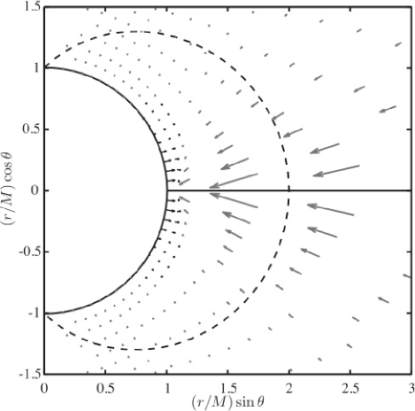
Figure 1: Time-averaged energy transport in the disk-black hole system. The electromagnetic disturbance is given by Eq. (43) with the wave frequency $\omega\simeq 0.76238\Omega_{\rm H}$, and the spin parameter a is chosen as $a=0.99999M$. The arrows show the poloidal energy flux with the components $\langle{\cal E}^{r}\rangle$ and $\sqrt{\Delta}\langle{\cal E}^{\theta}\rangle$, which are normalized by $\psi_{0}^{\ 2}/M^{4}$. The dark gray and light gray arrows correspond to the fluxes with $\langle{\cal E}^{r}\rangle>0$ and $\langle{\cal E}^{r}\rangle<0$, respectively. The horizon and the equatorial disk are shown as solid lines, and the boundary of the ergosphere is shown as a dashed line.

As the first application of $\psi$ given by Eq. (43) the time-averaged poloidal energy flow is shown in Fig. 1. The radial and zenithal components measured in an orthonormal basis may be given by $\sqrt{\Sigma/\Delta}\langle{\cal E}^{r}\rangle$ and $\sqrt{\Sigma}\langle{\cal E}^{\theta}\rangle$, respectively. In Fig. 1, however, the poloidal components expressed by the arrows correspond to $\langle{\cal E}^{r}\rangle$ and $\sqrt{\Delta}\langle{\cal E}^{\theta}\rangle$. This allows us to see the finite energy flux $\langle{\cal E}^{r}\rangle_{\textrm{H}}$ on the horizon. We note that see the finite energy flux $\langle{\cal E}^{r}\rangle_{\textrm{H}}\geq 0$ on the horizon is limited to the range $-\theta_{\textrm{m}}\leq\theta-\pi/2\leq\theta_{\textrm{m}}$ where $\theta_{\textrm{m}}\simeq 0.69743$. It is easy in Fig. 1 to see that the energy flux from the horizon in the range $-\theta_{\textrm{m}}<\theta-\pi/2<\theta_{\textrm{m}}$ is transported to the disk surface.

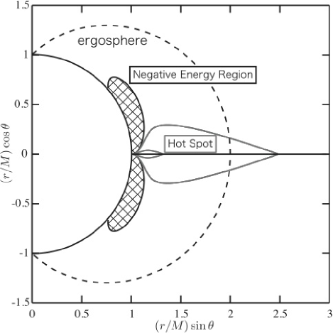
Figure 2: Contour of time-averaged energy density for the electromagnetic disturbance given by Eq. (43) on the $(r/M)\sin\theta$-$(r/M)\cos\theta$ plane. The wave frequency and the spin parameter are assumed to be $\omega\simeq 0.76238\Omega_{\rm H}$ and $a=0.99999M$ The negative energy region is shown as the shaded region. The position of the maximum energy density $\langle{\cal E}^{t}\rangle_{\textrm{m}}$ is at $r\simeq 1.0535M$. The surface giving $\langle{\cal E}^{t}\rangle=\langle{\cal E}^{t}\rangle_{\textrm{m}}/2$ (which may be explained as the boundary of the hot spot) is shown by the short gray line. To see the rapid decrease of $\langle{\cal E}^{t}\rangle$, the surface giving $\langle{\cal E}^{t}\rangle=\langle{\cal E}^{t}\rangle_{\textrm{m}}/10$ is also shown by the long gray line. The horizon and the equatorial disk are shown as solid line, and the boundary of the ergosphere is shown as a dashed line.

Next, let us consider the spatial distribution of the time-averaged energy density $\langle{\cal E}^{t}\rangle$ derived by the specific choice of $\psi(X)$. As will be seen Figs. 1 and 2, the region with $\langle{\cal E}^{t}\rangle<0$ is found to appear inside the region with $\langle{\cal E}^{r}\rangle>0$. It is also interesting to note that the energy density $\langle{\cal E}^{t}\rangle$ becomes maximum on the disk at the radius slightly apart from the horizon (i.e., at $r\simeq 1.0488r_{\rm H}$). The region with a high energy density such that $\langle{\cal E}^{t}\rangle\geq\langle{\cal E}^{t}\rangle_{\textrm{m}}/2$ (where $\langle{\cal E}^{t}\rangle_{\textrm{m}}$ is the maximum density) is shown in Fig. 2. If the deposited electromagnetic energy density dissipates to heat up the disk, a hot spot as expected to appear on the inner part of the disk including such a high energy density. As was mentioned in the previous section the energy flux (35) per unit area to illuminate the disk surface becomes maximum at the radius $r=4r_{\textrm{H}}/3$. The energy supply is also efficient in the inner part of disk near the horizon, and may balance the enrgy dissipation to keep the hot spot formation.

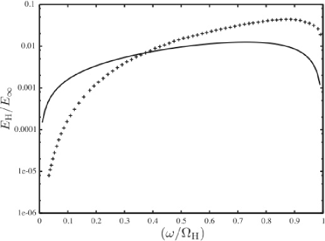
Figure 3: The efficiency $E_{\textrm{H}}/E_{\infty}$ of energy extraction in the disk-black hole system as a function of the wave frequency $\omega$ in the range $0<\omega<\Omega_{\textrm{H}}$. The spin parameter is fixed as $a=0.99999M$, to compare with the most efficient superradiant scattering amplification (corresponding to the mode $m=1$ and $\ell=1$) of vacuum electromagnetic waves estimated in Teukolsky and Press (1974), which is plotted by the points. The efficiency obtained from Eq. (43) is shown as a solid line.

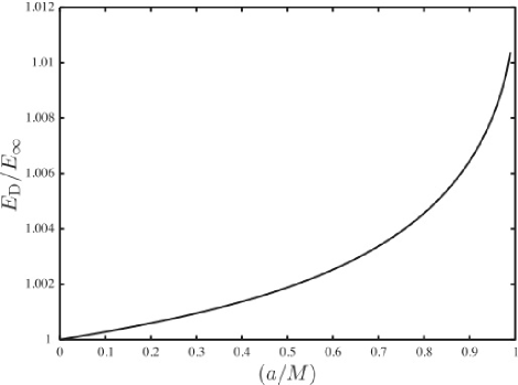
Figure 4: The efficiency $E_{\textrm{D}}/E_{\infty}$ of the disk illumination as a function of the spin parameter $a$. The wave frequency for the electromagnetic disturbance given by Eq. (43) is fixed as $\omega\simeq 0.76238\Omega_{\textrm{H}}$.

Finally let us calculate in more details the efficiency $E_{\textrm{H}}/E_{\infty}$ of the superradiant energy extraction from the black hole. In Fig. 3 the ratio $E_{\textrm{H}}/E_{\infty}$ is plotted as a function of the wave frequency $\omega$. We note that the maximum value of $E_{\textrm{H}}/E_{\infty}$ is much smaller than upper bound shown in Eq. (41). It may be possible to choose $\psi(X)$ allowing a more efficent energy extraction. Nevertheless we can claim from Fig. 3 that the efficiency $E_{\textrm{H}}/E_{\infty}$ obtained have can be larger (or not so smaller) than the efficiency of superradiant scattering without disk illumination evaluated in Teukolsky and Press (1974). It is sure that even though in the disk-black hole system the energy flux $\langle{\cal E}^{r}\rangle_{\textrm{H}}$ per unit area on the horizon becomes negative near the polar region, the net flux $E_{\textrm{H}}$ is not so suppressed. The energy extraction from the black hole induces the amplification of the disk illumination according to the conservation law (39). If the wave frequency is fixed to be $\omega\simeq 0.76238\Omega_{\textrm{H}}$ (corresponding to the maximum efficiency shown in Fig. 3, we can plot the efficiency $E_{\textrm{D}}/E_{\infty}$ of the disk illumination as a function of the spin parameter $a$. It is clear from Fig. 4 that $E_{\textrm{D}}/E_{\infty}$ increases monotonically as $a$ increases. If this result does not crucially depend on the specific choice of $\psi(X)$, we arrive at the conclusion that electromagnetic disturbance generated around a “near-extremal” black hole can most efficiently amplify the disk illumination.

Appendix A Extraction of angular momentum

Here let us discuss the relation between the energy flux and the angular momentum flux on the horizon. If the rotational energy is extracted from the black hole, then the angular momentum flux may be also extracted, which is defined by

$${\mathcal{L}}^{\mu}\equiv T^{\mu}_{\ \varphi}.$$ (44)

By using the same procedure to obtain $\langle{\cal E}^{r}\rangle_{\textrm{H}}$, the time-averaged radial angular momentum flux is given by

$$\langle{\mathcal{L}}^{r}\rangle_{\textrm{H}}=\langle{\mathcal{E}}^{r}\rangle_{\textrm{H}}/\Omega_{\textrm{H}}+\frac{a(1-\omega/\Omega_{\textrm{H}})^{2}\cos^{2}\theta}{4\pi r_{\textrm{H}}\Sigma_{\textrm{H}}\sin^{2}\theta}\langle|X\psi_{,X}|^{2}\rangle.$$ (45)

It is easy to see that the angular momentum on the horizon is extracted from the black hole, when the energy extraction occurs, i.e., $\langle{\mathcal{E}}^{r}\rangle_{\textrm{H}}>0$. However, if the net angular momentum flux $L_{\textrm{H}}$ on the horizon defined as

$$L_{\textrm{H}}\equiv\iint\langle{\mathcal{L}}^{r}\rangle_{\textrm{H}}\Sigma_{\textrm{H}}\sin\theta{\mathrm{d}}\theta{\mathrm{d}}\varphi.$$ (46)

is evaluated, we can recover the relation

$$E_{\textrm{H}}=\omega L_{\textrm{H}}.$$ (47)

Then, if the wave frequency $\omega$ is in the range $0<\omega<\Omega_{\textrm{H}}$, we obtain $L_{\textrm{H}}>0$. The angular momentum can be transported from the black hole to the disk via electromagnetic disturbances.

References

- Li (2002a) L.-X. Li, Astrophys. J 567, 463 (2002a).
- van Putten and Levinson (2003) M. H. P. M. van Putten and A. Levinson, Astrophys. J 584, 937 (2003).
- Blandford and Znajek (1977) R. D. Blandford and R. L. Znajek, Mon. Not. R. Astron. Soc. 179, 433 (1977).
- Li (2002b) L.-X. Li, Astron. Astrophys. 392, 469 (2002b).
- Gan et al. (2007) Z.-M. Gan, D.-X. Wang, and Y. Li, Mon. Not. R. Astron. Soc. 376, 1695 (2007).
- Wilms et al. (2001) J. Wilms, C. S. Reynolds, M. C. Begelnar, J. Reeves, S. Molendi, R. Staubert, and E. Kendziorra, Mon. Not. R. Astron. Soc. 328, L27 (2001).
- Tomimatsu and Takahashi (2001) A. Tomimatsu and M. Takahashi, Astrophys. J 552, 710 (2001).
- Uzdensky (2004) D. A. Uzdensky, Astrophys. J 603, 652 (2004).
- Uzdensky (2005) D. A. Uzdensky, Astrophys. J 620, 889 (2005).
- McKinney and Gammie (2004) J. C. McKinney and C. F. Gammie, Astrophys. J 611, 977 (2004).
- McKinney (2006) J. C. McKinney, Mon. Not. R. Astron. Soc. 368, 1561 (2006).
- Koide et al. (2006) S. Koide, T. Kudoh, and K. Shibata, Phys. Rev. D 74, 044005 (2006).
- Teukolsky and Press (1974) S. A. Teukolsky and W. H. Press, Astrophys. J 193, 443 (1974).
- Debney et al. (1969) G. C. Debney, R. P. Kerr, and A. Schild, J. Math. Phys. (N.Y.) 10, 1842 (1969).
- Burinskii et al. (2006) A. Burinskii, E. Elizalde, S. R. Hildebrandt, and G. Magli, Gravitation Cosmol. 12, 115 (2006), eprint astro-ph/0610036.