UNIVERSITÉ PARIS 11

THÈSE

Spécialité: PHYSIQUE THÉORIQUE

Présenté

pour obtenir le grade de
Docteur de l’Université Paris 11

par

Răzvan-Gheorghe Gurău

Sujet:

La renormalisation dans la théorie non commutative des champs

Soutenue le 19 décembre 2007 devant le jury composé de: $\begin{array}[]{lll}&\mbox{Jean Bernard Zuber}&\mbox{pr\'{e}sident}\\ &\mbox{Vincent Rivasseau}&\mbox{directeur de th\`{e}se}\\ &\mbox{Harald Grosse}&\mbox{rapporteur}\\ &\mbox{Edwin Langmann}&\mbox{rapporteur}\\ &\mbox{Jacques Magnen}&\mbox{examinateur}\end{array}$

Remerciements

Avant tout, je voudrais exprimer ma reconaissance á Vincent. Sans lui cette thèse n’aurait pas été possible. Il a été le meilleur directeur de thèse qu’on puisse avoir, non seulement pour ses calités scientifiques mais aussi pour ses qualités humaines. Au-delà de me former scientifiquement, il m’a appris l’ouverture, la rigueur et la critique (modérée par la bienveillance) et pour cela je lui serai endetté à jamais. Je ne pense pas avoir été le plus commode thésard, mais j’ai eu la chance et le privilège d’avoir été son élève. Il a toujours trouvé le temps de répondre à mes questions, même les plus bêtes, même répétées la dixième fois. Il a toujours préféré m’aider plutôt que me laisser me débrouiller tout seul. J’espère que notre collaboration se poursuivra par la suite, car il est pour moi un modéle humain et scientifique.

Je remercie à Jacques, de facto mon directeur de thèse adjoint. Nos collaborations m’ont appris surtout à ne jamais lâcher un problème. Il n’y a aucun problème trop difficile pour lui, et j’espère apprendre à lui ressembler. Sa fa con de toujours réduire un problème à l’essentiel, quoi qu’il devienne des fois difficile à suivre, est enviable. Après ces années passées ensemble j’espère avoir apris à utiliser mon intelect de la même fa con.

Je remercie à Jean Bernard Zuber, qui a eu la gentillesse d’accepter d’être le président de mon jury de thèse. Dans les trois années que nous avons enseigné ensemble le LP206 il m’a fait apprendre qu’il vaut mieux accepter les autres avant d’essayer à les améliorer. Je vous promets d’essayer de vous tutoyer!

A mes deux rapporteurs Harald Grosse et Edwin Langmann je voudrais les remercier d’avoir tout de suite accepté de faire partie de mon jury de thèse malgré les longues et peu commodes voyages qu’ils ont dû faire.

J’admire enormément les travaux de Harald Grosse, les travaux fondateurs pour les théories des champs non commutatives renormalisables. De ses travaux j’ai appris que la rigueur peut nous guider dans un labyrinthe de techniques et qu’il faut parfois faire un long calcul avant d’arriver à la compréhension. J’espère qu’en suivant son exemple je ne vais jamais me laisser intimidé par les dificultées techniques.

Les travaux d’Edwin Langmann sur la dualité Langmann-Szabo m’ont appris qu’il faut poursuivre des idées non standard et audacieuses pour leur beauté. De plus, les discussions avec lui ont ouvert mon intérêt pour les modèles matriciels que je voudrais approfondir dans le futur.

Je remercie Nikita Nekrasov qui a écrit un rapport sur ma thèse. Ses observations pertinentes m’ont amené a revoir et améliorer une partie de celle-ci. Il m’a aussi suggéré la référence [23] qui introduit un terme harmonique dans les théories noncommutatives sur le plan de Moyal. Ses très vastes travaux dans notre domaine montrent un esprit encyclopédique que j’espère acquérir un jour.

Je voudrais ensuite exprimer ma reconaissance à Monsier Gheorghe Nenciu, mon premier mentor. Les lectures qu’il m’a conseillées sont à la base de ma formation, et si jamais je trouve qu’une idée m’est familière c’est surtout grace à ses premiers conseils. Il est pour moi un example et un symbole d’honnêteté scientifique dans un contexte adverse. Ses encouragements ont beaucoup contribué à ma décision de continuer mes études en France et c’est pour cela aussi que je lui suis reconnaissant.

Je remercie à Madame Florina Stan qui m’a bénévolement enseigné les fondements de la physique. Pour avoir accepté de m’apprendre la physique à un moment très important de ma formation sans jamais demander rien en retour, elle reste pour moi une des grandes chances que j’ai eu.

Je voudrais aussi remercier à ma famille. Ma mère, mon père et ma soeur m’ont toujours soutenu dans ma decision de faire de la science. Ils ont toujours su m’aider et me conseiller, ainsi qu’à m’encourager de poursuivre mes idées. Ma décision d’apprendre la physique est dûe en grande partie à ma mère, qui a su me donner le bon livre à lire au bon moment de mon enface.

Je voudrais aussi exprimer mes remerciements à Marie-France Rivasseau pour avoir corrigé minutieusement le fran cais dans ma thèse. Si mon travail n’est pas présenté dans un fran cais parfait c’est uniquement dû aux corrections ajoutées après sa dernière lecture. Je voudrais aussi lui remercier de m’avoir si souvent re cu si chalereusement chez elle au cours de ces années.

Et surtout, je remercie à Delia. Elle a entiérement relu mon manuscrit et m’a énormérment aidé à mieux transmettre mes idees. Elle m’a toujours encouragé à me perfectionner, scientifiquement et personellement. Elle sait toujours me soutenir quand je passe des moments difficiles et je suis privilégié de l’avoir à mes côtés. Elle m’a appris à être plus fort et plus confiant en moi. Avoir arrivé aujord’hui à présenter ce travail est tout autant dû à la confiance qu’elle a eu en moi qu’à son effort et sacrifice chaque jour. C’est pour cela que cette thèse lui est dédiée.

Resumé

La théorie non commutative des champs est un candidat possible pour la quantification de la gravité. Dans notre thèse nous nous intéressons plus précisément au modéle $\phi^{4}$ sur le plan de Moyal dans un potentiel harmonique, introduit par Grosse et Wulkenhaar. Dans ce modèle la dualité de Langmann-Szabo présente au niveau du vertex est étendue au propagateur. Le long de nos études plusieurs résultats ont été obtenus concernant ce modèle. Nous avons ainsi prouvé la renormalisabilite à touts les ordres directement dans l’espace des positions. Nous avons introduit la représentation paramétrique du modèle, ainsi que la représentation de Mellin Complète. Nous avons prouvé que le flot de la constante de couplage est borné à tous les ordres de la théorie des perturbations. De plus nous avons introduit la régularisation et la renormalisation dimmensionelle du modèle. Les directions futures de recherche comprennent l’étude des théories de jauge sur le plan de Moyal et leur possible pertinence pour la quantification de la gravitation. Les liens avec la théorie des cordes et la gravitation quantique à boucles pourront aussi être détaillés.

Abstract

Non commutative quantum field theory is a possible candidate for the quantization of gravity. In our thesis we study in detail the $\phi 4$ model on the Moyal plane with an harmonic potential. Introduced by Grosse and Wulkenhaar, this model exhibits the Langmann-Szabo duality not only for the vertex but also for the propagator. We have obtained several results concerning this model. We have proved the renormalisability of this theory at all orders in the position space. We have introduced the parametric and Complete Mellin representation for the model. Furthermore we have proved that the coupling constant has a bounded flow at all orders in perturbation theory. Finally we have achieved the dimensional regularization and renormalization of the model. Further possible studies include the study of gauge theory on the Moyal plane and there possible applications for the quantization of gravity. The connections with string theory and loop quantum gravity should also be investigated.

Chapitre 1 Introduction

Aujourd’hui la physique est une des sciences les plus accomplies. Elle explique avec une précision remarquable les phénomènes les plus divers, sur une plage d’échelles comprise entre l’échelle du système solaire et l’échelle nucléaire. Entre ces deux limites les lois physiques fondamentales (la mécanique quantique, l’électromagnétisme, la gravitation, etc.) sont aussi bien prédictives que simples. Elles comportent un nombre réduit de paramètres et de postulats. Les phénomènes émergents, comme la chimie, la biologie, etc., sont très complexes à cause du grand nombre des constituants et non pas de la complexité des principes fondateurs.

La situation dégénère au fur et à mesure qu’on s’écarte de cette fenêtre d’énergies: on manque de modèles non seulement suffisamment prédictifs mais surtout mathématiquement satisfaisants. Le modèle standard, qui s’est imposé pour la description de la physique à petite échelle, a plus de $30$ paramètres indépendants et son Lagrangien est composé de plus de $100$ termes.

Toutes les théories physiques comprennent deux aspects: les lois valides à une certaine échelle d’énergie et la façon dont elles influencent les lois "effectives" à d’autres échelles d’énergie. Par exemple la mécanique quantique fournit une description presque parfaite des phénomènes à l’échelle atomique, mais il n’est pas raisonnable de l’appliquer directement au calcul de la pression d’un gaz dans une boîte. Pour ce calcul on doit utiliser la mécanique statistique classique.

Les phénomènes à l’échelle nucléaire sont décrits par la théorie des champs. Elle combine la mécanique quantique et la relativité restreinte (ce qui constitue un pas vers l’unification) et elle a une puissance prédictive impressionnante. L’histoire de la théorie des champs est remarquable en elle-même. Proposée dans les années $40$ elle a failli être abandonnée dans les années $60$ pour revenir en force dans les années $70$.

L’outil conceptuel le plus neuf de cette théorie est la renormalisation. Au début simple "recette de cuisine" utile pour cacher des quantités infinies dans des paramètres non physiques, la renormalisation est devenue un des concepts de base de notre compréhension de la physique à très courte échelle grâce à l’interprétation moderne à la Wilson.

Etant donné une théorie à une échelle d’énergie élevée, la renormalisation nous indique comment cette théorie se transforme à toutes les échelles d’énergie plus basses (donc à plus grande distance). Ainsi, il se peut que la structure de la théorie se reproduise, mais les valeurs de ses paramètres changent (et dans ce cas la théorie est dite renormalisable), ou il se peut que la théorie initiale engendre une autre théorie effective complètement différente.

Comme nous ne connaissons pas la théorie ultime, nous pouvons supposer qu’à une énergie très élevée on a un réservoir avec toutes les théories possibles. Si l’une de ces théories ne survit pas sur plusieurs échelles alors, plutôt qu’une véritable théorie universelle, elle est un accident du point de vue des autres échelles. Par contre, si la théorie se reproduit sur plusieurs échelles nous allons la rencontrer génériquement. Cette remarque nous mène à considérer de préférence des théories renormalisables pour décrire la physique.

Parmi les théories des champs possibles nous nous intéressons aux théories des champs sur des espaces non commutatifs (TCNC). Ces théories pourraient être adaptées à la description de la physique au-delà du modèle standard. De plus, elles sont certainement pertinentes pour la description de la physique en champ fort. La question de leur renormalisabilité est donc fondamentale pour savoir si ces théories sont génériques et universelles au sens décrit ci-dessus. C’est l’étude de cette question qui est le thème central de notre thèse.

Comme la renormalisation est une technique assez compliquée nous devons nous poser la question du niveau de rigueur des résultats que nous souhaitons avoir. Il y a trois niveaux de rigueur que nous pourrions nous proposer dans notre étude.

Un résultat peut être vérifié jusqu’à un certain ordre de la théorie de perturbations. C’est le niveau auquel s’arrête le physicien expérimentateur. Le modèle standard a été vérifié dans les expériences de haute énergie jusqu’à l’ordre trois au moins dans certains effets fins comme le calcul du facteur $g-2$ de l’électron prédit avec dix chiffres en électrodynamique quantique . Du point de vue du groupe de renormalisation la plus spectaculaire vérification est la variation de la constante de structure fine par deux pour cent sur la plage d’échelle accessibles aux expériences au LEP.

Le deuxième niveau de rigueur que nous pouvons nous proposer est de prouver un résultat à tous les ordres dans la théorie des perturbations. C’est le niveau du physicien théoricien, et c’est à ce niveau-ci que nous présentons tous les travaux de notre thèse.

Le troisième niveau est constructif. C’est le niveau ultime du physicien mathématicien. Il s’agit par exemple de prouver la ressommation au sens de Borel des séries de perturbations en une fonction, et ensuite d’étendre les propriétés prouvées pour la série à sa somme de Borel. Des développements récents prometteurs existent dans cette direction qui nous permettent d’espérer que la construction des modèles de théories des champs sur des espaces non commutatifs ne va pas tarder.

Dans le chapitre suivant nous présentons une introduction générale aux théories des champs sur des espaces non commutatifs. Le chapitre trois comprend une introduction générale au modèle $\Phi^{\star 4}_{4}$ sur l’espace de Moyal et présente d’autres modèles traités par nous. Les chapitres quatre à huit présentent différents résultats obtenus au cours de notre thèse. Le chapitre neuf présente les conclusions de cette thèse. Le chapitre dix présente quelques aspects techniques concernant le plan de Moyal. Les appendices contiennent les différents travaux qui sont à la base de nos résultats.

Chapitre 2 Historique et problématique des TCNC

L’idée de chercher une représentation géométrique nouvelle du monde à très petite échelle est bien plus ancienne qu’on ne pourrait le croire. Des idées dans ce sens ont été avancées par Schrödinger [1] dès l’année 1934. Reprises par Heisenberg [2], Pauli et Oppenheimer, ces idées sont pour la première fois formulées mathématiquement par Snyder [3]. Les études initiales ont été motivées d’une part par l’étude des particules dans des forts champs magnétiques et d’autre part par l’espoir que le comportement à petite échelle (UV) de telles théories sera amélioré.

Après ces travaux initiaux, l’idée de combiner une non-commutativité des coordonnées avec la physique a été longtemps négligée à cause principalement des difficultés mathématiques (notamment liées à l’invariance de Lorentz) et du développement spectaculaire des théories des champs commutatives.

Nous avons aujourd’hui plusieurs raisons de nous intéresser de nouveau aux TCNC. Nous les rencontrons comme candidates pour la physique des hautes énergies mais aussi comme une description naturelle de la physique des particules non relativistes dans un champ magnétique fort. L’effet Hall quantique découvert en 1980 par von Klitzing [4] a été l’une des plus grandes surprises de la physique moderne: les électrons dans un champ fort ont un comportement collectif qui conduit à la quantification de la résistance. L’effet Hall fractionnaire, mis en évidence par Tsui et Störmer [5] n’a pas été prévu par les théoriciens et il est encore plus surprenant. Les travaux théoriques sur ce sujet ont culminé avec l’introduction par Laughlin [6] d’une fonction d’onde non locale décrivant le liquide de Hall. Cette fonction d’onde peut être interprétée en termes d’un gaz d’anyons, des objets ayant des charges fractionnaires. Ces objets ont été mis en évidence expérimentalement sous la forme de bruit de grènaille (voir [7] pour une présentation détaillée). Dans ces expériences nous "voyons" en quelque sorte concrètement les charges fractionaires.

En plus de la description de Laughlin nous disposons d’une description d’un système de Hall en terms d’une théorie de champ de Chern Simons. Une interprétation de cette théorie en terme de particules composées formées d’électrons habillés avec des quanta du champ magnétique à été proposée par Read [8].

Les deux descriptions de l’effet Hall font intervenir des objets non locaux. Leur analyse devrait faire intervenir en conséquence des théories de champs non locales. La non-localité peut, à son tour, être traduite comme provenant d’une description non commutative de l’espace. Ces considérations ont mené Susskind [9] à conjecturer que l’effet Hall devrait être bien décrit par une théorie de Chern Simons non commutative. Ses travaux formels ont été affinés par Polychronakos [10] qui a proposé une version matricielle avec des coupures raides (sharp cutoffs) du modèle de Chern Simons non commutatif comme théorie finitaire utilisable dans la description de l’effet Hall. Van Raamsdonk et al. [11] ont mis en correspondance les états propres de la théorie de Polychronakos avec les fonctions d’onde de Laughlin. Ces idées sont à la base de l’étude des liquides non commutatives (voir [12] pour une présentation du sujet).

Nous espérons que le développement dans cette thèse du groupe de renormalisation adaptée aux TCNC s’appliquera à ces problèmes. Il n’existe pas encore une étude de la renormalisation des théories de champs qui s’appliquent à l’effet Hall. Les comportements à longue distance caractéristiques de l’effet Hall devraient pouvoir être compris en termes d’un flot du groupe de renormalisation. Une telle étude apporterait l’explication ab initio de l’effet Hall fractionnaire ainsi qu’une description précise et unifiée des transitions entre tous les plateaux de Hall.

La deuxième raison en faveur de l’étude des TCNC est la physique des hautes énergies. Nous allons maintenant nous concentrer sur les arguments apportés par cette physique car la bonne théorie de la gravitation quantique reste à ce jour le "Graal" de la physique théorique moderne.

Une fois le modèle standard formulé dans les années $70$ les physiciens ont commencé à se poser sérieusement le problème de la quantification de la gravitation. Après de nombreux efforts dans cette direction nous avons aujourd’hui plusieurs candidats pour cette théorie quantique de la gravitation. Parmi ces propositions la théorie des cordes et la gravité quantique à boucles sont les plus élaborées.

La théorie des cordes à été introduite dans les années $70$ par Veneziano comme théorie effective des interactions fortes. A partir des travaux de $1984$ de Green et Schwarz, qui prouvent l’absence d’anomalies, elle s’est imposée comme la proposition dominante dans la physique au delà du modèle standard. Les cordes supersymétriques semblent promettre une bonne théorie de la gravitation quantique. Le principal succès de cette théorie reste à ce jour la présence du graviton (particule de masse nulle et spin $2$) dans le spectre de la corde fermée. Ainsi elle nous fournit un formalisme qui unifie naturellement les champs de jauge avec les gravitons.

De plus l’entropie des trous noirs à été calculée par Strominger et Vafa [13] et ensuite Maldacena et al. [14]. Ce calcul, un grand succès de la théorie des cordes, est cependant limité à des trous noirs très particuliers ($Q\approx M$, appellée aussi quasi-extrémaux).

D’autre part, malgré de nombreux efforts dans ce sense, la seconde quantification de la théorie des cordes et l’identification du vide restent non complètement elucidés. La possibilité de vides multiples compatibles avec la phenoménologie actuelle (le problème du "paysage") rendent les prédictions physiques difficiles.

La gravité quantique à boucles renonce totalement aux notions géométriques habituelles et essaie de les retrouver comme engendrées dynamiquement. L’objet fondamental dans cette théorie sont les réseaux de spins. Nous essayons d’associer à chaque configuration d’un réseau de spins un espace-temps. Cette hypothèse, certes séduisante est très difficile à manipuler et donne difficilement des prédictions.

Parmi les avancées récentes dans la domaine de la gravité quantique on doit aussi mentionner les théories de la relativité modifiées comme la relativité doublement restreinte. Cette dernière rend compte d’une longueur minimale égale pour tous les observateurs, fixée à l’échelle de Planck. On ne dispose pas pour l’instant d’un schéma de quantification satisfaisant de telles théories.

Pour tous ces raisons une théorie mathematiquement plus simple qui rende compte d’une partie des caractéristiques des théories présentées auparavant serait fort souhaitable.

Les TCNC étudiées dans cette thèse sont un autre candidat à la quantification de la gravité. A cause de leur énorme succès expérimental les théories des champs commutatives sont notre point de départ. Nous voulons trouver une description des phénomènes reconstituant dans une certaine limite la théorie des champs commutative mais qui, en plus, prenne en compte des effets de la relativité générale.

La théorie mathématique de la géométrie non commutative a été développée dans les années 80-90 par des mathématiciens comme Alain Connes, Michel Dubois-Violette, John Madore, etc.. Leurs travaux mathématiques ont semblé au début peu liés à la physique.

Tout a changé dans les années 90. Plusieurs résultats de la théorie des cordes ont pointé vers un régime limite de la théorie de type IIA décrit par la théorie non commutative sur le plan de Moyal. Cela, et l’espoir de construire des théories automatiquement régularisées dans l’UV, a relancé la recherche sur les TCNC. Assez tôt Filk [17] s’est rendu compte que dans les nouvelles TCNC le secteur planaire a le même comportement que les théories commutatives. La renormalisation du secteur planaire de ces théories, qui contient une infinité de graphes, est donc nécessaire.

Les théories de jauge non commutatives sur le plan de Moyal ont attiré l’intérêt à partir des travaux de Martin et Sanchez-Ruiz en 1999 [18]. Des études ont été menées sur le tore non commutatif par Sheikh-Jabbari [19]. Les auteurs ont vérifié la renormalisabilité à une boucle de ces théories.

Ces travaux ont culminé avec les travaux de Seiberg et Witten en 1999 [20]. Ces auteurs ont donné une relation (strictement formelle) entre les théories de Yang-Mills non commutatives et les théories ordinaires. Cette relation a engendré une activité fébrile et de milliers des papiers sur le sujet. Dans la même période, les travaux de Maldacena [21] ont mis en relation la théorie des cordes et les théories de jauge maximalement supersymétriques. Nous voyons ainsi un triangle de relation se développer entre les théories des champs commutatives, les TCNC et la théorie des cordes.

D’autre part, dans les années 97 Chamseddine et Connes [22] ont trouvé une reformulation du modèle standard (au niveau classique) en terme d’un principe d’action spectrale sur une géométrie non commutative très simple. Leurs travaux ont inspiré un vif intérêt (spécialement du côté des mathématiciens) et les actions spectrales ont aujourd’hui une vie scientifique propre. Malgré l’incontestable réussite de condenser le modèle standard sous une forme très compacte ces travaux suivent encore les schémas de quantification habituelle. En particulier ils ne fournissent pas un nouveau groupe de renormalisation pour le traitement du modèle standard ni une compréhension nouvelle de la gravité quantique. En ce sens les action spectrales semblent être seulement le sommet d’un iceberg non commutatif encore largement à découvrir.

Les TCNC ont été ensuite mis en relation avec la M-théorie compactifiée sur des tores, et une étude approfondie des instantons et solitons dans les TCNC a été menée par Nekrasov [23]. En plus la géométrie non commutative s’est avérée un outil très puissant pour la quantification par déformation dans la théorie des cordes. L’étude des groupes et groupoïdes quantiques a été entreprise à l’aide de la géométrie non commutative.

Entre les années 1995 et 2000 les progrès rapides dans les TCNC amenèrent l’espoir de faire des calculs plus sûrs et plus poussés que dans la théorie des cordes. Les TCNC avaient été prouvées renormalisables à une et deux boucles et tout le monde supposait qu’elles le seraient à tous les ordres. Un papier de 2000 par Chepelev et Roiban [24] (révélé aujourd’hui faux) semblait dire que c’était vraiment le cas. On avait alors une reformulation élégante du modèle standard, et on commençait à comprendre très bien les théories de jauge non commutatives. Un compte-rendu de l’état des TCNC dans l’année 2001 se trouve dans [25].

Les premiers troubles sont apparus peu après le papier de Chepelev et Roiban. Minwalla, Van Raamsdonk et Seiberg [26] ont trouvé un problème qui avait échappé à ces auteurs: il existe des graphes non-planaires qui sont convergents UV grâce à certains facteurs oscillants mais qui, à cause de leur comportement IR, insérés dans des graphes plus grands engendrent des divergences (ce phénomène est expliqué en détail dans le chapitre suivant). Ces divergences ne sont pas renormalisables et portent le nom de mélange UV/IR. Malgré ce problème, le comptage de puissance de Chepelev et Roiban semblait être correct. On sait aujourd’hui que ce n’est pas le cas. Même leur théorème de comptage des puissances (sans preuve publiée) s’est révélé en fait erroné.

Le mélange UV/IR est un problème fondamental des TCNC. Toute théorie des champs réels va souffrir de ces divergences. Malgré de nombreux efforts afin de surmonter ce problème on n’a pas trouvé de solution satisfaisante pendant quelques années. Entre temps les TCNC ont été abandonnées par une bonne partie de la communauté des cordes.

Pourquoi revenir sur des théories qui semblent inconsistantes? Nous allons présenter un "Gedanken Experiment" en faveur des TCNC.

Commençons par un argument classique de mécanique quantique, présenté par Feynman. Quand nous mesurons la position d’une particule (supposons un électron) nous l’illuminons avec un photon. Nous observons le processus d’absorbtion du photon par l’électron.

La précision de la mesure de la position de l’électron est donnée par la longueur d’onde du photon. Cette limitation est due au fait que la probabilité de présence du photon est étendue sur une largeur spatiale donnée par sa longueur d’onde. Pour l’augmenter on doit utiliser des photons d’énergie de plus en plus haute. Les photons vont subir un choc avec les électrons, et vont leur communiquer une certaine impulsion. Comme le choc est élastique on ne peut pas affirmer avec précision quelle impulsion va être transférée entre les photons et les électrons. L’impulsion de transfert maximal nous donne l’incertitude sur l’impulsion de l’électron. Les photons avec de hautes énergies vont perturber l’impulsion de l’électron de plus en plus. Les deux mesures sont concurrentes: accroître la précision de la mesure de la position d’un électron va augmenter l’incertitude de la mesure de son impulsion. Nous sommes ainsi forcés d’introduire le principe d’incertitude de Heisenberg.

Toutes les théories qui essaient de décrire l’au-delà du modèle standard ont convergé sur l’idée qu’il existe une échelle fondamentale dans la nature où les effets de la quantification de la gravitation seront ressentis: l’échelle de Planck $\ell_{P}$. Le rapport entre cette échelle et l’échelle de la corde joue un rôle essentiel dans la théorie des cordes. En même temps c’est l’échelle unité du réseau de spin dans la gravitation quantique, et l’échelle invariante dans la relativité doublement restreinte.

Il est assez naturel de conjecturer qu’à cette échelle la nature même de l’espace-temps présente des changements profonds. Il devrait être impossible de localiser un objet avec une précision plus petite que la longueur de Planck. Ce qui est plus profond et moins évident au sujet de l’échelle de Planck c’est qu’elle est plus profondément une échelle d’aire qu’une échelle de longueur.

Faisons une expérience de pensée inspirée par l’expérience classique de Feynman. Nous voudrions mesurer la position d’un électron dans l’espace-temps. Supposons qu’on est loin de toute matière donc que l’espace temps est plat. Nous envoyons un photon (ou toute autre particule) dans la direction de l’électron. Nous essayons de mesurer la position de l’électron à l’aide de ce photon. La longueur d’onde associée à un photon libre d’énergie $E$ est $\lambda\approx hcE^{-1}$. C’est la précision maximale avec laquelle on peut localiser le photon dans sa direction de mouvement (et dans le temps). C’est ainsi la précision de la mesure de la position du point dans ces deux directions. Jusqu’ici on n’a pas innové par rapport à l’expérience de Feynman. Mais supposons maintenant qu’on veuille mesurer en même temps la position du point sur les directions transversales au mouvement du photon. A tout photon d’énergie $E$ on associe un rayon de Schwarzschild $r_{S}\approx GEc^{-4}$. Ce rayon représente l’horizon du photon. Aucune information (comme la position d’un électron à l’intérieur de cet horizon) ne peut le franchir. Ce que nous pouvons affirmer avec certitude c’est que le point est soit à l’intérieur soit à l’extérieur de l’horizon. Le rayon de Schwarzschild nous donne une borne sur la précision de la localisation du point sur les deux directions orthogonales au mouvement du photon. Comme $r_{S}$ augmente avec l’énergie, les mesures de la position d’un point sur les directions parallèles et orthogonales à son mouvement sont incompatibles!

Le produit de ces deux incertitudes est $\lambda r_{S}=\ell_{P}^{2}$. On ne peut pas sonder la géométrie sur des aires plus petites que cette aire fondamentale, le concept d’espace-temps continu doit être repensé!

Ce argument est classique et a été largement débattu au cours du temps. La principale critique qu’on lui a opposé c’est qu’il repose sur le préjugé que la relativité générale s’applique à des échelles où elle n’a jamais été testée. Cette critique n’est pas totalement fondée. En effet le seul ingrédient de relativité générale dont on s’est servi est la notion d’horizon. Cette notion est beaucoup plus large que la relativité générale. La thermodynamique des trous noirs, dont la théorie microscopique est gouvernée par une théorie quantique de la gravité encore à découvrir, est fondée sur cette notion.

La façon la plus simple d’engendrer un principe d’incertitude entre les positions est d’introduire la non-commutation des coordonnées (en tant qu’opérateurs quantiques):

$$[x^{i},x^{j}]=\imath\theta^{ij}\;,$$ (2.1)

où $\theta$ est une nouvelle constante analogue à la constante de Planck. Un espace de ce type porte le nom d’espace de Moyal. Nous pouvons évidemment essayer de traiter des commutateurs plus compliqués $\theta^{ij}(x)$.

Cet argument simple nous dit que les TCNC sont fondamentales pour la compréhension de la physique à l’échelle de Planck! Nous devons donc chercher des solutions afin de contourner les problèmes de ces théories comme le mélange UV/IR!

La solution du mélange a dû attendre les années 2003-2004 et les travaux fondateurs de Grosse et Wulkenhaar [27, 28, 29] portant sur le modèle $\phi^{4}_{4}$ sur l’espace de Moyal ${\mathbb{R}}^{4}$. Le vertex de cette théorie possède une symétrie non triviale: il a la même forme dans l’espace des positions et dans l’espace des impulsions. L’idée de Grosse et Wulkenhaar a été de modifier aussi le propagateur du modèle pour obéir à cette symétrie! Cette modification relie les régimes UV et IR au niveau de l’action libre et constitue la bonne solution du mélange. Grosse et Wulkenhaar ont pu prouver que le modèle $\Phi_{4}^{\star 4}$ ainsi modifié est renormalisable à tous les ordres de perturbation. Nous allons dorénavant appeler ce modèle vulcanisé.

Leurs travaux ont été ensuite repris et développés et la grande majorité des résultats de notre thèse porte sur ce sujet.

Nos études nous poussent à complètement changer notre intuition habituelle sur les petites et les grandes échelles. Il s’avére que penser aux échelles en termes de distance n’a plus de sens dans les TCNC: il y a une symétrie entre les comportements à longue et courte distance. Seul a un sens de parler de zones de haute et basse énergie. Comme l’énergie est bornée inférieurement on a une seule direction du groupe de renormalisation! Ce point de vue peut être qualifié de spectral, car on base notre analyse sur le spectre du hamiltonien. Il rejoint ainsi les idées de l’action spectrale et nous fournit probablement le bon cadre pour leur quantification future.

Nous pouvons adopter deux attitudes envers ce problème: soit essayer de trouver le plus vite possible le maximum de modèles ayant la symétrie de Langmann-Szabo et qui ne présentent pas de mélange, soit essayer de comprendre en plus grand détail la théorie $\Phi_{4}^{\star 4}$ et le nouveau groupe de renormalisation qui lui est associé. Le long de cette thèse nous allons prendre le deuxième point de vue. Nous espérons ainsi dégager le plus grand nombre de traits spécifiques des TCNC sur l’espace de Moyal, et développer une panoplie d’outils plus complète.

Parmi les modèles récents vulcanises de TCNC nous avons le modèle de Gross-Neveu étudié par Vignes-Tourneret [32] et des propositions de théories de jauge développées indépendemment par Grosse et al. [33], de Goursac et al. [34]. Tandis que le modèle de Vignes-Tourneret a été prouvé renormalisable nous ne disposons pas encore de preuve que les théories de jauge récemment proposé le soient. Le modèle $\Phi_{6}^{\star 3}$ a été prouvé renormalisable par Gross et Steinacker [35], et le modèle $\Phi_{3}^{\star 6}$ par Zhi Tuo Wang.

Le premier trait spécifique des TCNC est la non-localité. Comme la notion de point perd son sens il est inévitable de perdre la notion de localité. Cette perte et tous les problèmes correspondants d’unitarité et perte d’invariance sous le groupe de Poincaré font que les TCNC ont des difficultés à s’imposer dans la communauté des physiciens.

Cependant une non-commutation de type Moyal est covariante sous le groupe de Lorentz restreint. Nous considérons les TCNC comme une première étape en direction de la physique de l’échelle de Planck. Nous conjecturons qu’au fur et à mesure qu’on monte dans les énergies on va rencontrer des comportements de TCNC sur l’espace de Moyal qui seront ensuite remplacés par des comportements plus compliqués avec un paramètre $\theta$ qui deviendra sans doute dynamique, jusqu’à l’échelle de Planck où nous espérons atteindre une formulation réellement indépendante du fond.

Chapitre 3 Le modèle $\Phi^{\star 4}_{4}$

Nous voulons entreprendre une étude qui nous révèle avec précision le plus grand nombre des traits spécifiques des TCNC. Pour cela nous sommes forcés de choisir un espace non commutatif très simple. Par la suite nous allons nous placer sur l’espace de Moyal. Sa description précise se trouve dans l’appendix 10.1. En quelques mots, il s’agit de l’espace ${\mathbb{R}}^{D}$ muni d’un produit non commutatif de façon que le commutateur des deux coordonnées soit une constante.

3.1 Définition du modèle

Nous voulons généraliser le modèle $\Phi^{4}_{4}$ commutatif défini par l’action:

$$S=\int d^{D}x[\frac{1}{2}\partial_{\mu}\bar{\phi}(x)\partial_{\mu}\phi(x)+\frac{1}{2}\mu^{2}\bar{\phi}(x)\phi(x)+\frac{\lambda}{4!}\bar{\phi}(x)\phi(x)\bar{\phi}(x)\phi(x)]\;,$$ (3.1)

qui décrit un boson chargé muni d’une interaction à quatre corps.

Dans un premier temps on va simplement remplacer les produits par des produits de Moyal:

$$S=\int d^{D}x[\frac{1}{2}\partial_{\mu}\bar{\phi}(x)\star\partial^{\mu}\phi(x)+\frac{1}{2}\mu^{2}\bar{\phi}\star\phi(x)+\frac{\lambda}{2}\bar{\phi}\star\phi\star\bar{\phi}\star\phi(x)]\;,$$ (3.2)

où $\star$ est le produit de Moyal défini par (10.1).

Une propriété (10.5) du produit de Moyal est que dans toute intégrale quadratique on peut le remplacer par le produit habituel. Par conséquent la partie libre de l’action est celle habituelle (commutative), la différence entre ce modèle et le modèle correspondant commutatif provenant exclusivement du terme d’interaction (explicité en eq. (10.1)).

Pour un champ scalaire réel, le modèle naïf souffre d’un nouveau type de divergence: le mélange ultraviolet infrarouge. Il existe un graphe (appelé tadpole non planaire pour des raisons qui seront plus claires par la suite), représenté dans la figure 3.1, qui est convergent ultraviolet, mais qui, enchaîné un nombre arbitraire de fois dans une boucle, engendre une divergence infrarouge aussi forte que l’on veut.

Figure 3.1: Le tadpole nonplanaire

Son amplitude à impulsion de transfert $p$ est:

$${\cal A}\propto\int d^{4}k\frac{e^{ip_{\mu}k_{\nu}\theta^{\mu\nu}}}{k^{2}+\mu^{2}}\simeq_{p\to 0}p^{-2}\;,$$ (3.3)

et l’on peut engendrer une puissance négative de $p$ toute aussi grande que l’on désire! Cette divergence ne peut pas être réabsorbée dans la redéfinition des paramètres initiaux de la théorie et rend la théorie non renormalisable.

Ce type de divergence s’avère être très générique dans la TCNC. Non seulement elle est présente dans toutes les théories réelles définies sur l’espace de Moyal, mais elle est aussi présente pour des théories définies sur des variétés non commutatives plus générales.

Il est vrai que ce mélange n’est pas présent dans une théorie complexe, car les graphes comme le tadpole non planaire ne sont pas permis dans un tel modèle, mais cette solution n’est pas satisfaisante. C’est plutôt un accident dû aux règles de contraction qu’une solution de principe.

Malgré de nombreux efforts sur ce sujet, le mélange n’a pu être résolu qu’avec l’introduction par Grosse et Wulkenhaar d’une modification de l’action initiale du modèle.

Le vertex de ce modèle possède une symétrie non triviale: son expression dans l’espace des impulsions et des positions est identique! On appelle cette symétrie la dualité de Langmann-Szabo. La percée de Grosse et Wulkenaar consiste dans l’addition d’un nouveau terme quadratique dans l’action pour rendre covariante sous cette transformation aussi la partie libre du modèle. Le modèle de $\Phi^{\star 4}_{4}$ "vulcanisé" qui sera analysé en détail tout le long de cette thèse est donc décrit par l’action:

$$S=\int d^{D}x[\frac{1}{2}\partial_{\mu}\bar{\phi}\star\partial^{\mu}\phi+\frac{1}{2}\Omega^{2}\tilde{x}^{2}\bar{\phi}\star\phi+\frac{1}{2}\mu^{2}\bar{\phi}\star\phi+\frac{\lambda}{2}\bar{\phi}\star\phi\star\bar{\phi}\star\phi]\;,$$ (3.4)

avec $\tilde{x}=2\theta^{-1}x$.

Les études initiales de ce modèle ont été menées dans la base matricielle (BM) introduite dans l’appendice 10.1. Nous présentons par la suite un bref survol des principaux résultats obtenus par ces méthodes.

3.2 L’action dans la BM

L’action (3.4) s’écrit dans la base matricielle comme:

$$S=2\pi\theta\sum_{m,n,k,l}\Big{(}\bar{\phi}_{mn}H_{mn,kl}\phi_{kl}+\frac{\lambda}{2}\bar{\phi}_{mn}\phi_{nk}\bar{\phi}_{kl}\phi_{lm}\Big{)}\,,$$ (3.5)

ou par $\bar{\phi}$ on a noté la matrice hermitienne conjuguée de $\phi$. Les indices $m$, $n$, etc. sont des paires de nombres entiers positifs $m=(m^{1},m^{2})\in{\mathbb{N}}^{2}$.

La partie quadratique de l’action est donnée par (voir [28]):

$$H_{mn,kl} = \Big{[}\mu^{2}+\frac{2(1+\Omega^{2})}{\theta}(m+n+1)\Big{]}\delta_{nk}\delta_{ml}-\frac{2(1-\Omega^{2})}{\theta}$$ (3.6)

$$\times \Big{[}\sqrt{(n+1)(m+1)}\delta_{n+1k}\delta_{m+1l}+\sqrt{nm}\delta_{n-1k}\delta_{m-1l}\Big{]}\;.$$

L’inverse de la partie quadratique est le propagateur. La grande réussite technique de Grosse et Wulkenhaar consiste dans le calcul explicite de ce propagathor, faisant intervenir des familles de polynômes orthogonaux.

Une preuve alternative et directe de leur résultat se trouve en appendice A. Le calcul rèpose sur l’astuce de Schwinger. Nous représentons la matrice inverse par l’intégrale:

$$H^{-1}=\frac{\theta}{8\Omega}\int_{0}^{1}\frac{d\alpha}{1-\alpha}(1-\alpha)^{\frac{\theta}{8\Omega}H}\,.$$ (3.7)

Les seuls éléments matriciels non nuls sont donnés par:

$$[(1-\alpha)^{\frac{\theta}{8\Omega}H}]_{mm+h,l+hl}=$$

$$\sum_{u=max(0,-h)}^{min(m,l)}A(m,l,h,u)\Big{(}C\frac{1+\Omega}{1-\Omega}\Big{)}^{m+l-2u}E(m,l,h,u)\;,$$ (3.8)

avec $C=\frac{(1-\Omega)^{2}}{4\Omega}$, et

$$A(m,l,h,u)=\frac{\sqrt{m!(m+h)!l!(l+h)!}}{(m-u)!(l-u)!(h+u)!u!}$$

$$E(m,l,h,u)=\frac{(1-\alpha)^{\frac{h+2u+1}{2}}\alpha^{m+l-2u}}{(1+C\alpha)^{m+l+h+1}}\;.$$ (3.9)

3.2.1 Les graphes de Feynman

Le modèle (3.5) est un modèle dit "pseudomatriciel". Les graphes de Feynman d’un tel modèle sont beaucoup plus riches en information topologique que ceux du modèle commutatif. Comme le propagateur lie deux indices à deux autres, nous le représentons par un ruban (voir fig. (3.2)).

Figure 3.2: Le propagateur et le vertex dans l’espace des matrices

De même, le vertex est représenté comme un carrefour de quatre rubans (voir fig. 3.2). Les graphes de Feynman de ce modèle ressemblent à ceux d’un modèle matriciel à la différence que les indices ne sont pas parfaitement conservés le long des rubans.

Prenons l’exemple des deux tadpoles, présenté dans la figure 3.3.

Figure 3.3: Le tadpole planaire et non planaire

Pour le premier tadpole l’indice $d$ est sommé sur la boucle interne et les indices $a$, $b$ et $c$ sont des indices externes. Pour le deuxième tous les indices sont des indices externes. Le tadpole dans la partie gauche de la figure a une face interne (avec indice de face $d$) et une face brisée par des pattes externes. Nous l’appelons "planaire". Le tadpole de droite a deux faces brisées et nous l’appelons (de manière impropre) non-planaire.

Tout graphe avec $N$ vertex, $L$ propagateurs et $F$ faces dont $B$ brisées par les $N_{e}$ pattes externes peut être dessiné sur une surface de Riemann de genre $g$, donné par:

$$2-2g=N-L+F\;.$$ (3.10)

et avec $B$ frontières.

A chaque ligne on associe une orientation de $\bar{\phi}$ à $\phi$. Autour d’un vertex les flèches entrantes et sortantes se succèdent. A cause de cette propriété le modèle est appelé orientable. Séparons les deux bords d’un ruban en bord droit et bord gauche par rapport à cette orientation.

Pour un graphe donné, son complexe conjugué est donné par le graphe ayant toutes les flèches renversées. Dans le graphe complexe conjugué tous les bords droits sont devenus gauches et inversement.

Le propagateur de ce modèle est réel, et le vertex aussi. Par conséquent nous devons toujours extraire la partie réelle des fonctions de corrélation. Nous symétrisons toujours un graphe et son complexe conjugué. Par conséquent notre modèle a une symétrie parfaite entre la gauche et la droite.

Une notion très importante est celle de "graphe dual". A tout "graphe direct" on associe le graphe ayant toutes les faces remplacées par des vertex et tous les vertex par des faces. Ainsi nous le construisons de la manière suivante:

• A toute face on associe son vertex dual.

• A chaque indice que l’on rencontre en tournant autour de la face on associe un coin sur le vertex dual.

• Tout propagateur de $mn$ à $kl$ est remplacé par son dual allant de $mk$ à $nl$.

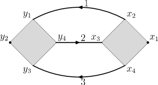
L’exemple du graphe "sunshine" et de son dual est présenté dans la figure 3.4.

Figure 3.4: Le sunshine et son dual

Les caractéristiques topologiques du graphe ${\cal G}$ dual de $G$ sont:

$${\cal N}({\cal G})=F(G),\quad{\cal F}({\cal G})=N(G),\quad{\cal L}({\cal G})=L(G),$$

$${\cal N}_{e}({\cal G})=B(G),\quad{\cal B}({\cal G})=N_{e}(G),\quad\gamma({\cal G})=g(G)\;,$$ (3.11)

où nous avons noté en calligraphique le nombre de vertex, faces et lignes du graphe dual et avec $\gamma$ son genre.

3.2.2 Comptage de puissances

On s’intéresse à établir le comptage de puissances de ce modèle. D’une manière opportune on se place à $\Omega=1$, où le modèle devient purement matriciel. Cela signifie que dans la figure 3.4 on a $m_{1}=m_{2}$ et $n_{1}=n_{2}$. Nous devons par conséquent sommer un indice par face. Les modifications à $\Omega\neq 1$ seront indiquées au long du texte.

Nous décomposons les propagateurs en tranches:

$$\frac{1}{m+n+A}=\int_{0}^{\infty}dte^{-t(m+n+A)}=\sum_{i=0}^{\infty}C^{i}\;,$$ (3.12)

avec

$$C^{i}=\int_{M^{-(i+1)}}^{M^{-i}}dte^{-t(m+n+A)}\leq M^{-i}e^{-KM^{-i}(m+n+A)}\;.$$ (3.13)

Nous voulons sommer tous les indices de faces, à attribution des indices de tranches donnée (la somme sur les attributions est facile).

Pour tout graphe, considérons son dual. Il sera très important par la suite. Les indices des faces du graphe direct sont maintenant associés aux vertex du graphe dual.

A attribution d’échelle donnée, nous notons à l’étage $i$ les composantes connexes $G_{k}^{i}$ du graphe formé par toutes les lignes avec des indices supérieurs ou égaux à $i$. Il est facile de prouver que si un graphe n’est pas connexe alors son dual ne l’est pas non plus.

Supposons que le dual de $G_{k}^{i}$, noté ${\cal G}_{k}^{i}$, n’est pas connexe. Alors $G_{k}^{i}$ ne sera pas connexe non plus, ce qui est faux. Nous concluons que les composantes connexes à l’échelle $i$ du graphe dual ${\cal G}_{k}^{i}$ sont les duaux des composantes connexes $G_{k}^{i}$ du graphe direct à l’échelle $i$.

Les préfacteurs des propagateurs donnent:

$$\prod_{\ell}M^{-i_{\ell}}=\prod_{i;k}M^{-{\cal L}({\cal G}_{k}^{i})}\;.$$ (3.14)

Tout indice sommé avec la décroissance d’un propagateur d’échelle $i$ va nous coûter $M^{2i}$. Nous avons donc intérêt à sommer les indices avec les propagateurs les plus infrarouges possible.

Appellons ${\cal J}$ l’ensemble des propagateurs qu’on utilise pour sommer. Pour le construire commençons par la plus basse tranche. Parmi les lignes qui ont l’échelle exactement égale à $i$, on choisit toutes les lignes de tadpole et l’on efface les vertex sur lesquels elles se branchent. Ensuite on choisit le maximum des lignes qui relient des vertex, à condition qu’elles ne forment pas des boucles. Une fois qu’un maximum de lignes de l’échelle $i$ a été choisi nous passons à l’échelle $i+1$.

On obtient ainsi l’ensemble ${\cal J}$ des lignes les plus infrarouges tel que tout vertex ait une ligne de tadpole, ou bien soit relié au reste des vertex par une ligne d’arbre.

Ensuite nous analysons notre graphe des hautes échelles vers les basses. Pour autant qu’un vertex porte encore des demi-lignes non contractées nous ne sommons pas son index. A l’échelle où toutes les demi-lignes du vertex se branchent sur des propagateurs nous sommons son index avec la ligne de l’ensemble ${\cal J}$ qui le touche. Les sommes nous coûtent:

$$\prod_{\ell\in{\cal J}}M^{2i_{\ell}}=\prod_{i,k}M^{2[{\cal N}({\cal G}_{k}^{i})-{\cal N}_{e}({\cal G}_{k}^{i})]}\;.$$ (3.15)

En mettant ensemble (3.14) et (3.15) et en passant aux nombres topologiques du graphe direct on obtient:

$$\prod_{i,k}M^{-4g(G_{k}^{i})-2[B(G_{k}^{i})-1]-\frac{N_{e}(G_{k}^{i})-4}{2}}\;.$$ (3.16)

Nous pouvons maintenant comprendre pourquoi cette théorie ne possède pas le mélange UV/IR.

Dans la théorie non vulcanisée on ne peut pas sommer les indices avec des lignes de tadpole du graphe dual. Nous ne devons choisir dans ${\cal J}$ que des lignes d’arbre. Supposons qu’à l’échelle basse $i$ les demi lignes d’un vertex se branchent dans un tadpole. Nous sommes obligés de sommer son index avec une ligne d’arbre qui est d’échelle plus élevée $j$. La contribution totale est donc:

$$M^{-i}M^{-j}M^{2j}=M^{j-i}\;,$$ (3.17)

qui n’est pas sommable sur $j$ par rapport à $i$. Une telle contribution divergente, ayant plus d’une face brisée n’a pas la forme du lagrangien et ne peut pas être renormalisée!

Dans notre théorie, par contre, c’est possible de sommer avec les lignes de tadpole du graphe dual. On somme toujours un vertex avec la ligne la plus infrarouge qui le touche! Par conséquent, pour l’exemple ci-dessus on a:

$$M^{-i}M^{-j}M^{2i}=M^{-(j-i)}\;,$$ (3.18)

qui est sommable sur $j$ par rapport à $i$.

3.2.3 Renormalisation dans la BM

Le comptage de puissances établi dans la section précédente nous dit que les contributions divergentes viennent seulement des sous fonctions planaires avec une seule face brisée avec deux ou quatre pattes externes :

$$g(G_{k}^{i})=0,\quad B(G_{k}^{i})=1,\quad N_{e}(G_{k}^{i})=2\text{ ou }4\;.$$ (3.19)

Nous notons $\Gamma^{4}(m,n,k,l)$ la fonction à quatre points, planaire avec une seule face brisée, une particule irréductible amputée avec indices externes $m$, $n$, $k$ et $l$.

Nous notons $\Sigma(m,n)$ la fonction à deux points, planaire avec une seule face brisée, une particule irréductible amputée avec des indices externes $m$ et $n$.

Nous effectuons un développement de Taylor de la fonction à quatre points:

$$\Gamma^{4}(m,n,k,l)=\Gamma^{4}(0,0,0,0)+m\partial_{m}\Gamma^{4}+\dots\;.$$ (3.20)

Le premier terme de la relation ci-dessus est logarithmiquement divergent. Pour le soustraire il suffit de rajouter dans l’action un contre-terme de la forme:

$$\Gamma^{4}(0,0,0,0)\bar{\phi}_{mn}\phi_{nk}\bar{\phi}_{kl}\phi_{lm}\;.$$ (3.21)

La fonction à deux points a un développement de Taylor de la forme:

$$\Sigma(m,n)=\Sigma(0,0)+(m+n)\partial\Sigma(0,0)+\dots\;,$$ (3.22)

où l’on a noté $\partial\Sigma$ la dérivée de $\Sigma$ par rapport à un de ses indices externes (à cause de la symétrie gauche droite on peut choisir librement l’index par rapport auquel on dérive). Cette dérivée fait intervenir les fonctions à deux points avec un saut d’index sur les pattes externes.

La fonction à deux points s’écrit comme:

$$G^{2}(m,n)=H_{mn,nm}-\Sigma(0,0)-(m+n)\partial\Sigma(0,0)\;,$$ (3.23)

et on reconnaît dans le premier terme une renormalisation quadratique de la masse et dans le deuxième une renormalisation logarithmique de la fonction d’onde .

3.3 Autres modèles dans la BM

Nous voulons étendre les méthodes présentées dans ce chapitre à des modèles plus généraux. Nous voulons traiter un système de particules dans un champ magnétique constant. Cette étude devrait être pertinente pour l’effet Hall. De plus, l’invariance par translation n’est pas brisée dans ces théories, car les translations sont remplacées par des translations magnétiques. Suite à cette étude nous allons pouvoir déterminer si la vulcanisation peut être réinterprétée comme la présence d’un champ externe constant ou non.

Nous ne connaissons pas la forme de l’interaction entre les particules adaptée à l’effet Hall. En effet la littérature est très peu précise à ce sujet. Le consensus est que les interactions ne devraient pas jouer de rôle pour l’effet Hall entier mais qu’elles sont essentielles pour l’effet Hall fractionnaire. Cela dit, l’effet Hall fractionnaire ne repose pas sur la forme précise de l’interaction, il suffit d’avoir une interaction décroissante avec la distance pour l’obtenir.

Nous pourrions être tentés de prendre comme interaction celle de Coulomb, traduite par l’échange de photons. Certes, cette interaction est l’interaction fondamentale entre les électrons. Cependant, comme il s’agit de particules non relativistes il est raisonnable de supposer que l’interaction effective est différente. Nous supposons que cette interaction est à quatre corps. Le point de vue darwinien que nous adoptons dans cette thèse nous mène à considérer toutes les interactions qui sont juste renormalisables dans l’ultraviolet, étant ainsi des points fixes du groupe de renormalisatoin. Une fois achevée l’étude détaillée du propagateur, nous allons tester si les interactions de type Moyal entrent dans cette catégorie.

La partie quadratique de l’action est simple. Dans la jauge symétrique, la dérivée covariante est:

$$D_{\mu}=\partial_{\mu}+\imath\Omega\tilde{x}_{\mu}\;,$$ (3.24)

et le hamiltonien libre devient:

$$H_{\Omega}=-\frac{1}{2}D_{\mu}D_{\mu}=\frac{1}{2}\left(-\partial^{2}+4\frac{\Omega^{2}}{\theta^{2}}x^{2}+2\imath\frac{\Omega}{\theta}x\wedge\partial\right)\;.$$ (3.25)

Nous pouvons en effet analyser un modèle encore plus général, avec le Hamiltonien libre donné par:

$$H_{B}=\frac{1}{2}\left(-\partial^{2}+4\frac{\Omega^{2}}{\theta^{2}}x^{2}+2\imath\frac{B}{\theta}x\wedge\partial\right)\;.$$ (3.26)

L’étude détaillée du propagateur d’un tel modèle fait l’objet du travail présenté en annexe A.

Pour mener l’analyse en tranches de ce propagateur nous obtenons les représentations suivantes dans l’espace direct et dans la BM:

Lemma 3.3.1

Si H est:

$$H_{B}=\frac{1}{2}\big{[}-\partial_{0}^{2}-\partial_{1}^{2}+\Omega^{2}x^{2}-2\imath B(x_{0}\partial_{1}-x_{1}\partial_{0})\Big{]}.$$ (3.27)

Le noyau intégral de l’opérateur $e^{-tH}$ est:

$$e^{-tH_{B}}(x,x^{\prime})=\frac{\Omega}{2\pi\sinh\Omega t}e^{-A},$$ (3.28)

$$A=\frac{\Omega\cosh\Omega t}{2\sinh\Omega t}(x^{2}+x^{\prime 2})-\frac{\Omega\cosh Bt}{\sinh\Omega t}x\cdot x^{\prime}-\imath\frac{\Omega\sinh Bt}{\sinh\Omega t}x\wedge x^{\prime}.$$ (3.29)

Et dans la base matricielle on a:

Lemma 3.3.2

$$(1-\alpha)^{\frac{\theta}{8\Omega}H_{B}}_{mm+h,ll+h}=(1-\alpha)^{\frac{\theta}{8\Omega}H}_{mm+h,ll+h}(1-\alpha)^{-\frac{B}{2\Omega}h}\;.$$ (3.30)

Grâce à la simplicité du vertex de Moyal dans la BM, on peut espérer prouver la renormalisabilité de tels modèles de TCNC une fois que le comportement d’échelle de ce propagateur a été détaillé dans la BM.

Les principaux résultats de l’annexe A sont les suivants:

• Nous trouvons toujours une décroissance d’ordre $1$ dans l’indice $l-m$. Les indices sont très bien conservés le long des rubans. Les modèles avec un tel propagateur sont pseudo-matriciels.

• A $B\neq\Omega$ le comportement est semblable à celui à $B=0$. Nous avons une décroissance d’ordre $M^{i}$ dans l’indice $h=n-m$ (l’écart entre les bords des rubans) ce qui nous permet de reproduire le comptage de puissance de $\phi_{4}^{\star 4}$. Dans cette catégorie entre le modèle $LSZ$ général.

• Pour $\Omega=B$ la situation change drastiquement. Un modèle de ce type est le modèle de Gross-Neveu de [32]. Le comportement d’échelle est gouverné par un point col non-trivial dans l’espace d’indices de matrice. Dans la région d’indices près de ce col on perd les décroissances d’échelle en $h$. Il s’avère que le seul cas pour lequel cette perte est dangereuse est le "sunshine".

Le traitement de [32] est mené dans l’espace direct. Le propagateur n’a pas de décroissance dans $v^{2}$ mais seulement une oscillation $e^{\imath\Omega u\wedge v}$. Un tel facteur oscillant nous permet en principe d’affirmer que $u\wedge v\approx 1$ (et nous donne le bon ordre de grandeur pour $v$) à l’aide des intégrations par parties. Les intégrations par partie requises pour chaque graphe sont décrites en détail dans [32]. Ces oscillations du propagateur doivent être combinées avec les oscillations des vertex. Il faut choisir un ensemble de variables indépendantes par rapport auxquelles on effectue les intégrations par partie.

Nous rencontrons le "problème du sunshine" à $\Omega=1$. Les oscillations des vertex compensent exactement celles des propagateurs! Cette compensation fait que nous ne pouvons pas obtenir le bon comptage des puissances. Dans l’espace des matrices le statut spécial de ce point peut être vu comme la rencontre du premier niveau de Landau. Dans la base matricielle le propagateur devient:

$$C_{mn}=\frac{1}{m}\;,$$ (3.31)

et on n’a aucune décroissance en $n$!

Nous pouvons conclure que le point $\Omega=1$ a un statut très spécial pour ces modèles: la renormalisabilité de ces modèles à $\Omega=1$ est remise en question.

Nous n’avons pas trouvé pour l’instant une façon de découper ce propagateur en tranches dans l’espace direct ou dans la base matricielle adaptée à l’étude du point $\Omega=1$. Des progrès récents dans cette direction ont été faits par Disertori et Rivasseau, mais on manque encore de preuves que ces modèles à $\Omega=1$ soient renormalisables.

En effet il s’avère que ces problèmes sont génériques. Nous les rencontrons chaque fois que nous essayons de traiter la vulcanisatoin comme une pure dérivée covariante dans un champ externe constant.

Si les termes de vulcanisation ne sont pas engendrés par un champ de fond, quelle est donc leur origine? De plus, si l’on ne peut pas absorber la brisure de l’invariance par translation dans un changement de jauge, est-ce que ces théories peuvent être vraiment physiques?

Pour répondre à ces questions nous pensons que la clé est de trouver un modèle fermionique du type modèle de Gross-Neveu, vulcanisé sans singularité à $\Omega=1$. Une proposition de théorie fermionique est détaillée dans les conclusions. Malheureusement, pour l’instant ces théories brisent l’invariance par translation.

Chapitre 4 Renormalisation dans l’espace direct

Dans ce chapitre nous présentons une preuve alternative de la renormalisabilité de la théorie $\Phi^{\star 4}_{4}$.

Pourquoi a-t-on besoin d’une nouvelle preuve de la renormalisabilité? Il y a plusieurs arguments en faveur d’une telle démarche.

À cause de la complexité du propagateur dans la base matricielle, la preuve dans cette dernière est très technique. Nous souhaiterions avoir une preuve plus simple.

Plus important, la renormalisabilité d’une théorie repose sur deux caractéristiques: le comptage de puissances et la forme des contre-termes. Le comptage de puissances est assez transparent dans la base matricielle, mais la forme des contre-termes n’est pas du tout transparente. Qu’est-ce qui remplace le principe de localité pour notre théorie? L’étude qui suit nous mène à introduire un principe de Moyalité qui est la bonne généralisation de cette notion.

En $D=4$ le propagateur dans l’espace direct est [36]:

$$C(x,x^{\prime})=\int_{0}^{\infty}dt\frac{\Omega^{2}}{[2\pi\sinh\Omega t]^{2}}e^{-\frac{\Omega}{4}\coth\frac{\Omega t}{2}(x-x^{\prime})^{2}-\frac{\Omega}{4}\sinh\frac{\Omega t}{2}(x+x^{\prime})^{2}-\mu_{0}^{2}t}\;,$$ (4.1)

et le vertex [17] peut se représenter comme:

$$V(x_{1},x_{2},x_{3},x_{4})=\delta(x_{1}-x_{2}+x_{3}-x_{4})e^{i\sum_{1\leqslant i<j\leqslant 4}(-1)^{i+j+1}x_{i}\theta^{-1}x_{j}}\;,$$ (4.2)

avec $x\theta^{-1}y\equiv\frac{2}{\theta}(x_{1}y_{2}-x_{2}y_{1}+x_{3}y_{4}-x_{4}y_{3})$.

La partie interaction de l’action est réelle. On représente le vertex comme dans l’équation (4.2), mais on devrait se rappeler que la somme des parties imaginaires est nulle. De plus, le vertex est invariant sous la transformation $1\leftrightarrow 3$ et $2\leftrightarrow 4$.

La fonction $\delta$ du vertex nous impose que les quatre champs soient positionnés dans les coins d’un parallélogramme. Le facteur d’oscillation fait intervenir l’aire du parallélogramme. Il la contraint à être d’ordre $\theta$.

La valeur de $\theta$, le commutateur des deux coordonnées, nous donne en terme de mécanique quantique la plus petite aire qu’on peut mesurer. Il est donc naturel de trouver que l’interaction de quatre champs est maximale quand ils se distribuent sur une surface d’aire minimale admise.

Pour tout propagateur nous introduisons une variable "courte" $u$ (et une "longue" $v$) égale à la différence (somme) entre les positions des deux extrémités du propagateur. Dans la zone ultraviolette ($t\approx M^{-2i}$) on a $u\approx M^{-i}$ et $v\approx M^{i}$. Ces variables sont centrales pour la suite.

Nous avons déjà vu que dans l’espace direct les vertex sont représentés par des parallélogrammes. Chaque parallélogramme est muni d’un sens de rotation correspondant à l’ordre cyclique des quatre coins. Pour représenter un graphe nous représentons tous ses vertex avec le même sens de rotation (trigonométrique) sur un plan et ensuite nous branchons les propagateurs représentés par des lignes.

4.1 Le comptage de puissances

Le propagateur de la théorie $\Phi^{4}_{4}$ commutative est borné dans une tranche par:

$$C^{i}\leq M^{2i}e^{-M^{i}|u|}\;.$$ (4.3)

Le comptage de puissance est neutre car tout vertex a en moyenne deux propagateurs, donc un préfacteur $M^{4i}$ et un point à intégrer, ce qui nous rapporte $M^{-4i}$.

Pour la théorie $\Phi^{\star 4}_{4}$, nous décompossons le propagateur (à masse nulle) comme:

$$C=\sum_{i}C^{i}\quad C^{i}=\int_{M^{-2(i+1)}}^{M^{-2i}}dt\frac{\Omega^{2}}{[2\pi\sinh\Omega t]^{2}}e^{-\frac{\Omega}{4}\coth\frac{\Omega t}{2}u^{2}-\frac{\Omega}{4}\sinh\frac{\Omega t}{2}v^{2}}\;,$$ (4.4)

et le propagateur dans une tranche est borné par:

$$C^{i}\leq M^{2i}e^{-M^{i}|u|-M^{-i}|v|}\;.$$ (4.5)

Tout vertex a en moyenne deux propagateurs comme avant, donc un facteur $M^{4i}$, et nous devons intégrer deux variables courtes et deux variables longues. Nous utilisons la fonction $\delta$ pour intégrer l’une des variables longues. Nous obtenons $M^{-8i}$ pour les intégrales courtes et $M^{4i}$ pour l’intégrale longue: le comptage de puissances est de nouveau neutre.

Cette argument doit être affiné pour une attribution d’échelle générale (de nouveau la somme sur les attributions est simple). Choisissons un arbre qui est compatible avec l’attribution d’échelle . En intégrant les variables longues de l’arbre avec les fonctions $\delta$ et en bornant les facteurs oscillants par $1$, l’amplitude d’un graphe ${\cal A}$ est bornée par:

$${\cal A}_{G} \leq\prod_{\ell\in G}M^{2i_{\ell}}\prod_{\ell\in T}M^{-4i_{\ell}}=\prod_{i,k}M^{2L(G_{k}^{i})}\prod_{i,k}M^{-4[N(G_{k}^{i})-1]}$$ (4.6)

$$=\prod_{i,k}M^{-[N_{e}(G_{k}^{i})-4]}\;,$$

car pour toutes les lignes de boucle le facteur obtenu par l’intégration de la variable longue compense exactement celui de la variable courte.

Il faut améliorer ce comptage de puissance pour obtenir les modifications dues à la topologie du graphe. Pour cela l’on doit exploiter les facteurs oscillants des vertex. Ils s’expriment à l’aide d’une opération topologique, appelée premier mouvement de Filk.

Soit une ligne du graphe qui joint deux vertex. Nous réduisons cette ligne et nous collons les deux vertex adjacents dans un seul grand vertex. Cette opération conserve le sens de rotation des vertex. Itérons cette opération pour toutes les lignes d’un arbre dans le graphe pour aboutir à un graphe réduit, appelé rosette, formé d’un seul vertex ayant uniquement des lignes de tadpole (un exemple est présenté dans la figure 4.1).

Figure 4.1: Premier mouvement de Filk: la ligne $2$ est réduite et les vertex se collent.

Cette opération ne modifie ni le genre $g$, ni le nombre de faces $F$, ni le nombre de faces brisées $B$ du graphe. Si le graphe est non-planaire il y aura un croisement des deux lignes de la rosette (voir par exemple 4.2).

Figure 4.2: Une rosette nonplanaire

A un tel croisement correspond un facteur oscillant $e^{\imath v_{a}\wedge v_{b}}$ entre les variables longues des deux lignes de boucle ($e^{\imath v_{2}\wedge v_{4}}$ dans Fig: 4.2). Si, avant de borner l’oscillation par $1$, on utilise ce facteur pour intégrer la variable $v_{2}$ on arrive à gagner un facteur $M^{-4i_{a}}$ ($M^{-4i_{2}}$ dans Fig. 4.2) au lieu de payer un facteur $M^{4i_{b}}$ ($M^{4i_{4}}$ dans Fig. 4.2), ce qui rend toute fonction non-planaire convergente. Un argument similaire nous donne l’amélioration due aux faces brisées. Nous obtenons ainsi, directement dans l’espace direct, un comptage de puissance partiel de la théorie, suffisant pour prouver la renormalisabilité.

4.2 Les soustractions

Nous venons de comprendre dans le nouveau contexte pourquoi seules les fonctions planaires à une seule face brisée avec deux ou quatre pattes externes sont divergentes. Il faut maintenant comprendre pourquoi ces divergences ont la forme du Lagrangien initial. Qu’est-ce qui remplace la notion de localité dans notre théorie?

Soit une fonction divergente à quatre points. Si tous les propagateurs internes sont très ultraviolets leurs extrémités sont presque confondues. Dans ces conditions la fonction est un pavage planaire de parallélogrammes. Ils vont forcément avoir la forme d’un parallélogramme entre les points externes! De plus l’aire orientée du parallélogramme résultant est la somme des aires orientées des parallélogrammes. La fonction réproduit précisément la forme du produit de Moyal! Un exemple est présenté dans la figure 4.3.

Figure 4.3: Un pavage divergent

En termes mathématiques cela se traduit par le lemme suivant:

Lemma 4.2.1

La contribution de vertex d’un graphe planaire à une face brisée peut s’exprimer sous la forme:

$$\delta(\sum_{i}(-1)^{i+1}x_{i}+\sum_{l\in T\cup{\cal L}}u_{l})e^{\imath\sum_{i,j}(-1)^{i+j+1}x_{i}\theta^{-1}x_{j}}$$

$$e^{\imath\sum_{l\in T\cup{\cal L},\;l\prec j}u_{l}\theta^{-1}(-1)^{j}x_{j}+\imath\sum_{l\in T\cup{\cal L},\;l\succ j}(-1)^{j}x_{j}\theta^{-1}u_{l}}$$

$$e^{-\imath\sum_{l,l^{\prime}\in T\cup{\cal L},\;l\prec l^{\prime}}u_{l}\theta^{-1}u_{l^{\prime}}-\imath\sum_{l\in T}\frac{u_{l}\theta^{-1}v_{l}}{2}\varepsilon(l)-\imath\sum_{l\in{\cal L}}\frac{u_{l}\theta^{-1}w_{l}}{2}\varepsilon(l)}$$

$$e^{-\imath\sum_{l\in{\cal L},\,l^{\prime}\in{\cal L}\cup T;\;l^{\prime}\subset l}u_{l^{\prime}}\theta^{-1}w_{l}\varepsilon(l)}\ ,$$ (4.7)

où $T$ est l’arbre réduit et ${\cal L}$ est l’ensemble des lignes de boucle.

Dans la première ligne du lemme ci-dessus on reconnaît la forme du noyau du produit de Moyal. Nous effectuons un développement de Taylor dans la deuxième ligne ci-dessus. Tous les termes correctifs font intervenir au moins une insertion d’une variable courte $u$, ce qui les rend sous-dominants. Comme la fonction à quatre points est logarithmiquement divergente l’on peut négliger les contributions sous-dominantes. Nous concluons que la partie divergente de la fonction a quatre points reproduit bien le produit de Moyal.

La fonction à deux points est plus compliquée. Elle se divise dans la contribution des tadpoles qui sont de la forme:

$${\cal A}=\int dudv\,\delta(x_{1}-x_{2}+\sum u)e^{\imath x_{1}\theta^{-1}x_{2}}F(u,v)\;,$$ (4.8)

et les autres contributions qui peuvent être mises sous la forme:

$${\cal A}=\int dudv\,\delta(x_{1}-x_{2}+\sum u)\delta(-x_{2}+\sum u+\sum v)F(u,v)\;.$$ (4.9)

Nous allons effectuer un développement de Taylor des contributions du haut. Commençons par les tadpoles:

$${\cal A} = \delta(x_{1}-x_{2})e^{\imath x_{1}\theta^{-1}x_{2}}\int dudv\,F(u,v)$$ (4.10)

$$+ \delta^{\prime}(x_{1}-x_{2})e^{\imath x_{1}\theta^{-1}x_{2}}\int dudv\,(\sum u)F(u,v)$$

$$+ \delta^{\prime\prime}(x_{1}-x_{2})e^{\imath x_{1}\theta^{-1}x_{2}}\int dudv\,(\sum u)(\sum u)F(u,v)\;.$$

Toutes les intégrales du haut sont gaussiennes. Par conséquent, le second terme est nul.

Le premier terme est une contribution locale, de masse, quadratiquement divergente. Le dernier terme est une contribution logarithmiquement divergente. Pour voir à quel opérateur ce dernier correspond nous allons lisser l’amplitude avec des fonctions test:

$$\int dx_{1}dx_{2}\,\delta^{\prime\prime}(x_{1}-x_{2})\,e^{\imath x_{1}\theta^{-1}x_{2}}\bar{\phi}(x_{1})\phi(x_{2})$$

$$=\int dx_{1}dx_{2}\,\delta(x_{1}-x_{2})\left(\partial_{1}+\imath\theta^{-1}x_{2}\right)^{2}\bar{\phi}(x_{1})\phi(x_{2})\;.$$ (4.11)

Cet opérateur n’est pas de la forme du lagrangien initial. La subtilité consiste à comprendre qu’il faut combiner ce tadpole avec son complexe conjugué. En effet, comme notre modèle est réel, il est naturel de toujours combiner les graphes avec leurs complexes conjugués. D’une manière équivalente, l’on peut brancher un même graphe sur la combination réelle des patte externes comme:

$$\int dx_{1}dx_{2}\,\delta(x_{1}-x_{2})\left(\partial_{1}+\imath\theta^{-1}x_{2}\right)^{2}[\bar{\phi}(x_{1})\phi(x_{2})+\phi(x_{1})\bar{\phi}(x_{2})]\;.$$ (4.12)

En dévéloppant l’expression ci-dessus, nous trouvons que la somme des deux tadpoles nous fournit un contre-terme pour l’opérateur:

$$\partial^{2}+\frac{1}{\theta^{2}}x^{2}\;.$$ (4.13)

Nous devons maintenant effectuer un développement de Taylor des autres contributions à la fonction à deux points:

$${\cal A} = \int dudv\,\delta(x_{1}-x_{2}+\sum u)\delta(-x_{2}+\sum u+\sum v)F(u,v)$$

$$= \delta(x_{1}-x_{2})\int dudv\,\delta(\sum u+\sum v)F(u,v)$$

$$+ \delta(x_{1}-x_{2})(-x_{2})\int dudv\,\delta^{\prime}(\sum u+\sum v)F(u,v)$$

$$+ \delta(x_{1}-x_{2})x_{2}^{2}\int dudv\,\delta^{\prime\prime}(\sum u+\sum v)F(u,v)$$

$$+ \delta^{\prime}(x_{1}-x_{2})\int dudv\,(\sum u)\delta(\sum u+\sum v)F(u,v)$$

$$+ \delta^{\prime}(x_{1}-x_{2})(-x_{2})\int dudv\,(\sum u)\delta^{\prime}(\sum u+\sum v)F(u,v)$$

$$+ \delta^{\prime\prime}(x_{1}-x_{2})\int dudv(\sum u)(\sum u)\delta(\sum u+\sum v)F(u,v)\;.$$

Le premier terme ci-dessus est une renormalisation de masse. Le deuxième est nul à cause du fait que $F(u,v)$ est gaussienne. Le troisième est une renormalisation de l’opérateur $x^{2}$. Le quatrième est nul dû de nouveau au fait que $F(u,v)$ est gaussienne. Le dernier est une renormalisation du $p^{2}$.

Nous analysons maintenant le cinquième terme. De nouveau, nous combinons un graphe avec son complexe conjugué. L’opérateur correspondant prend la forme:

$$\int\delta^{\prime}(x_{1}-x_{2})(-x_{2})[\bar{\phi}(x_{1})\phi(x_{2})+\phi(x_{1})\bar{\phi}(x_{2})]$$ (4.15)

$$= \int(-x)[\partial\bar{\phi}\phi+\bar{\phi}\partial\phi]=\int\bar{\phi}\phi\;,$$

et nous concluons qu’il est une sous-divergence de masse.

Nous avons ainsi prouvé que la fonction à deux points nous donne uniquement des contre-termes de la forme du Lagrangien initial.

A l’aide des mêmes techniques nous pouvons prouver que le modèle LSZ est renormalisable. La seule différence vient du fait que les noyaux des propagateurs ne sont pas réels, ce qui fait que les graphes ne se combinent pas exactement avec leurs complexes conjugués et nous avons par conséquent aussi une renormalisation du terme $\partial\wedge x$.

Chapitre 5 La fonction bêta du modèle $\Phi^{\star 4}_{4}$

Pour toute théorie des champs, nous nous intéressons uniquement aux fonctions de corrélation. Pour les exprimer, nous commencons en imposant un cutoff qui rend toute quantité finie. En suite, nous essayons de prendre la limite du cutoff tendant vers l’infini.

En effectuant le développement perturbatif, nous exprimons les fonctions de corrélation en fonction des paramètres nus de notre théorie. Nous rencontrons des contributions qui divergent avec le cutoff. La renormalisatoin absorbe ces divergences dans une rédéfinition des paramètres nus. Ainsi nous réexprimons les fonctions de corrélation en fonction des contributions renormalisées (finies) et des paramètres effectifs (également finis). Une fois la renormalisabilité d’une théorie établie, la question naturelle qui se pose est d’étabir la variation des paramètres effectifs avec le cutoff. Les flots des différents paramètres sont caractérisés par leurs fonctions bêta.

Pour notre modèle, le couplage effectif est donné par la fonction à quatre points, une particule irréductible, amputée $\Gamma^{4}$. A tout vertex correspondent deux propagateurs. Le couplage effectif est donné par:

$$\lambda_{i-1}=\frac{\Gamma^{4}_{i}}{Z^{2}_{i}}\;,$$ (5.1)

où $Z$ est la renormalisation de la fonction d’onde. Pour une théorie avec un cutoff ultraviolet $\Lambda$, on peut décrire l’évolution du couplage effectif avec l’échelle à l’aide de la fonction $\beta(\lambda)$ définie comme:

$$\beta(\lambda)=\frac{d\lambda^{nu}}{d\ln\Lambda}\Big{|}_{\lambda^{ren}=ct.}\;.$$ (5.2)

Alternativement, dans le cadre de l’analyse multi-échelle nous préférons la définition:

$$\beta(\lambda)_{i}=\lambda_{i-1}-\lambda_{i}\;.$$ (5.3)

Pour la théorie $\Phi^{4}_{4}$ commutative le couplage effectif évolue avec l’échelle. Cette évolution est assez facile à comprendre au premier ordre. Nous avons une contribution non nulle pour la fonction $\Gamma^{4}$ provenant des boules. Le tadpole, étant local, est un contre-terme de masse, et $Z=1$ à une boucle.

Une étude détaillée nous montre que, si l’on veut une constante renormalisée non nulle nous devons commencer avec une constante nue grande. En effet le couplage nu devient infini pour un cutoff UV fini. Inversement, toute constante nue finie donne naissance à une théorie libre triviale dans l’infrarouge. Ceci est un grave problème dans la théorie des champs commutative et a reçu le nom "fantôme de Landau". Les infinis qu’on élimine par la renormalisation ressurgissent dans cette nouvelle divergence.

Ce problème a failli tuer la théorie des champs. Grâce à l’universalité de ce phénomène on l’a presque abandonnée comme description des interactions fondamentales. L’issue de cette situation n’apparaît qu’avec la découverte de la liberté asymptotique dans les théories de jauge non abéliennes. Mais même cette solution n’est pas entièrement satisfaisante. La liberté asymptotique est le fantôme renversé. Cette fois-ci c’est la théorie ultraviolette qui devient triviale!

Il est vrai qu’une théorie libre dans l’ultraviolet est beaucoup plus physique qu’une théorie à couplage fort dans l’ultraviolet, et cela a permis notamment l’introduction du modèle standard pour les interactions fondamentales, néanmoins des problèmes subsistent. La convergence des flots du modèle standard vers une seule constante de couplage demande l’altération des flots. Cela peut être réalisé à l’aide de la supersymétrie, mais il n’y a eu aucune détection des partenaires supersymétriques jusqu’à maintenant.

De plus, ce même fantôme a empêché la construction du modèle $\Phi^{4}_{4}$ commutatif. Bien qu’on puisse penser que la théorie constructive des champs soit plutôt un jeu mathématique qu’une question physique, il n’empêche que sans elle les calculs perturbatifs n’ont pas de sens. Si l’on ne peut pas construire une théorie des champs, la série perturbative risque d’être fausse à partir du premier ordre!

Nous concluons donc que les flots des modèles de théories des champs commutatives posent un problème profond et les rendent mathématiquement malades.

La situation change complètement dans les TCNC. Pour le modèle $\Phi^{\star 4}_{4}$ le tadpole n’est plus local! Il nous donne une renormalisation non triviale de la fonction d’onde à partir du premier ordre. Les calculs à une boucle effectués par Grosse et Wulkenhaar [37] nous donnent un flot du paramètre $\Omega$ vers $1$ et à cette valeur le flot du couplage s’arrête. Ce résultat a été généralisé jusqu’à trois boucles par Disertori et Rivasseau en [38].

Ces résultats ouvrent la porte vers une possibilité tentante. Est-il possible que le flot de cette théorie soit borné sans que la théorie soit triviale? Dans ce cas on aurait une théorie bien définie et non triviale tout au long de sa trajectoire sous le (semi-)groupe de renormalisation! Pour le reste du chapitre nous nous plaçons à $\Omega=1$.

Nous avons le théorème suivant:

Theorem 5.0.1

L’équation:

$$\Gamma^{4}(0,0,0,0)=\lambda(1-\partial\Sigma(0,0))^{2}$$ (5.4)

est vraie aux corrections irrelevantes près à tous les ordres de perturbation, soit comme équation entre les quantités nues avec cutoff UV fixé ou comme équation entre les quantités renormalisées. Dans ce dernier cas $\lambda$ est la constante nue exprimée comme série en puissances de $\lambda_{ren}$.

Prouver un tel résultat est dans un certain sens très difficile. Il faut prouver qu’il est vrai à tous les ordres de perturbation, et ensuite constructivement! Comme nous allons le voir par la suite, la preuve de la validité à tous les ordres de perturbation est en effet beaucoup plus simple que prévu.

Elle repose sur deux idées: les identités de Ward et l’équation de Dyson. Nous allons travailler dans la base matricielle. Comme $\Omega=1$, nous avons:

$$C_{mn;kl}=C_{mn}\delta_{ml}\delta_{nk}\ ;\ C_{mn}=\frac{1}{A+m+n}\ ,$$ (5.5)

avec $A=2+\mu^{2}/4$, $m,n\in\mathbb{N}^{2}$ et

$$\delta_{ml}=\delta_{m_{1}l_{1}}\delta_{m_{2}l_{2}}\ ,\qquad m+n=m_{1}+m_{2}+n_{1}+n_{2}\ .$$ (5.6)

La fonctionnelle génératrice est

$$Z(\eta,\bar{\eta})=\int d\phi d\bar{\phi}\leavevmode\nobreak\ e^{-S(\bar{\phi},\phi)+F(\bar{\eta},\eta,;\bar{\phi},\phi)}$$

$$F(\bar{\eta},\eta;\bar{\phi},\phi)=\bar{\phi}\eta+\bar{\eta}\phi$$

$$S(\bar{\phi},\phi)=\bar{\phi}X\phi+\phi X\bar{\phi}+A\bar{\phi}\phi+\frac{\lambda}{2}\phi\bar{\phi}\phi\bar{\phi}$$ (5.7)

où les traces sont sous-entendues et $X_{mn}=m\delta_{mn}$. $S$ est l’action et $F$ sont les sources externes.

5.1 Les identités de Ward

Nous rappelons l’orientation des propagateurs de $\bar{\phi}$ à $\phi$. Pour un champ $\bar{\phi}_{ab}$ l’indice $a$ est un indice gauche et $b$ un indice droit. Le premier (second) indice de $\bar{\phi}$ se contracte toujours avec le second (premier) indice de $\phi$. Par conséquent pour $\phi_{cd}$, $c$ est un indice droit et $d$ est un indice gauche.

Soit $U=e^{\imath B}$ avec $B$ une matrice petite hermitienne. Nous faisons un changement de variable “gauche" (car il agit seulement sur les indices gauches)

$$\phi^{U}=\phi U;\bar{\phi}^{U}=U^{\dagger}\bar{\phi}\ .$$ (5.8)

Comme il s’agit d’un simple changement de variable, nous avons:

$$\partial_{\eta}\partial_{\bar{\eta}}\frac{\delta\ln Z}{\delta B_{ba}}=0\;,$$ (5.9)

avec $\eta$ des terms de source. En explicitant cette relation on trouve pour les fonctions planaires à deux points l’identité de Ward:

$$(a-b)<[\bar{\phi}\phi]_{ab}\phi_{\nu a}\bar{\phi}_{b\nu}>_{c}=<\phi_{\nu b}\bar{\phi}_{b\nu}>_{c}-<\bar{\phi}_{a\nu}\phi_{\nu a}>_{c}\;.$$ (5.10)

(les indices répétés ne sont pas sommés).

Figure 5.1: L’identité de Ward pour les fonctions à 2p points avec insertion sur une face gauche.

Les indices $a$ et $b$ sont des indices gauches, et notre identité de Ward décrit des fonctions avec une insertion sur la face gauche, comme dans la figure 5.1. Il est possible d’obtenir une identité similaire avec l’insertion sur la face droite. De plus, en dérivant davantage par rapport aux sources externes nous pouvons obtenir de telles identités avec un nombre arbitraire de pattes externes.

Cette équation a été déduite de l’intégrale fonctionnelle. Elle est donc vraie ordre par ordre dans la théorie des perturbations, car celle-ci se déduit à partir de l’intégrale fonctionnelle.

On a l’habitude de regarder les identités de Ward comme conséquences de l’invariance de jauge. Dans notre traitement on obtient une identité de Ward comme conséquence d’une invariance du vertex sous un changement de variable qui ne laisse pas invariante la partie quadratique. Peut-on interpréter ce changement de variable comme une invariance de jauge?

Le premier pas dans cette direction est d’introduire des opérateurs covariants de multiplication $X$ qui se transforment sous le changement de variable comme:

$$X^{U}=U^{\dagger}XU\;.$$ (5.11)

Il faut ensuite construire une action invariante sous cette transformation, telle que sa forme fixée de jauge soit (5). Cette invariance sera l’invariance habituelle d’un modèle de matrice sous les transformations unitaires.

Nous devrons de plus utiliser ces "transformations de jauge" pour construire une théorie de Yang-Mills associée aux théories non commutatives vulcanisées. Elle sera très certainement différente des théories Yang-Mills vulcanisées proposées par [33] et [34], car dans leurs travaux seulement les champs $\phi$ et $\bar{\phi}$ changent sous les transformations de jauge.

5.2 L’équation de Schwinger Dyson

Nous introduisons maintenant le deuxième outil conceptuel dont nous avons besoin pour prouver le théorème (5.0.1).

Soit $G^{4}(m,n,k,l)$ la fonction à quatre points connexe planaire avec une face brisée avec $m$, $n$, $k$ et $l$ les index de la face externe dans l’ordre cyclique. Le premier index $m$ est toujours choisi comme index gauche.

Soit $G^{2}(m,n)$ la fonction à deux points connexe avec indices externes $m,n$ (appelé aussi propagateur habillé). Comme d’habitude, $\Sigma(m,n)$ est la fonction à deux points, une particule irréductible, amputée. $G^{2}(m,n)$ et $\Sigma(m,n)$ sont liées par:

$$G^{2}(m,n)=\frac{C_{mn}}{1-C_{mn}\Sigma(m,n)}=\frac{1}{C_{mn}^{-1}-\Sigma(m,n)}\,.$$ (5.12)

Soit $G_{ins}(a,b;...)$ la fonction connexe à deux points planaire à une face brisée avec une insertion sur la face gauche avec saut d’index de $a$ à $b$. L’identité de Ward (5.10) s’écrit comme:

$$(a-b)\leavevmode\nobreak\ G^{2}_{ins}(a,b;\nu)=G^{2}(b,\nu)-G^{2}(a,\nu)\,.$$ (5.13)

Figure 5.2: L’équation de Dyson

Analysons $G^{4}(0,m,0,m)$. Soit une patte externe $\bar{\phi}$ et le premier vertex qui lui est attaché. En tournant vers la droite sur le bord $m$ à ce vertex nous rencontrons une nouvelle ligne (marquée dans la figure 5.2). Cette ligne peut soit séparer le graphe en deux composantes déconnectées ($G^{4}_{(1)}$ et $G^{4}_{(2)}$ dans 5.2) soit non ($G^{4}_{(3)}$ dans 5.2). De plus, si cette ligne sépare le graphe en deux composantes disconnectées, le premier vertex peut soit appartenir à la composante à deux pattes ($G^{4}_{(1)}$ dans 5.2) soit à la composante à quatre pattes ($G^{4}_{(2)}$ dans 5.2).

Cela est une simple classification des graphes: les composantes représentées dans la figure 5.2 prennent en compte leurs facteurs combinatoires. Nous pouvons donc écrire l’équation de Dyson:

$$G^{4}=G^{4}_{(1)}(0,m,0,m)+G^{4}_{(2)}(0,m,0,m)+G^{4}_{(3)}(0,m,0,m)\,.$$ (5.14)

Le terme $G^{4}_{(2)}$ est zéro par renormalisation de masse. $G^{4}_{(1)}+G^{4}_{(3)}$ donne $\Gamma^{4}=\lambda(1-\partial\Sigma)^{2}$ après amputation des propagateurs externes.

Nous allons analyser ici en détail la contribution $G^{4}_{(1)}$. Elle est de la forme:

$$G^{4}_{(1)}(0,m,0,m)=\lambda C_{0m}G^{2}(0,m)G^{2}_{ins}(0,0;m)\,.$$ (5.15)

Mais, par l’identité de Ward:

$$G^{2}_{ins}(0,0;m) = \lim_{\zeta\rightarrow 0}G^{2}_{ins}(\zeta,0;m)=\lim_{\zeta\rightarrow 0}\frac{G^{2}(0,m)-G^{2}(\zeta,m)}{\zeta}$$ (5.16)

$$= -\partial_{L}G^{2}(0,m)\,.$$

En utilisant la forme explicite du propagateur on a $\partial_{L}C^{-1}_{ab}=\partial_{R}C^{-1}_{ab}=\partial C^{-1}_{ab}=1$. En utilisant l’équation (5.12), on conclut:

$$G^{4}_{(1)}(0,m,0,m) = \lambda C_{0m}\frac{C_{0m}C^{2}_{0m}[1-\partial_{L}\Sigma(0,m)]}{[1-C_{0m}\Sigma(0,m)](1-C_{0m}\Sigma(0,m))^{2}}$$ (5.17)

$$= \lambda[G^{2}(0,m)]^{4}\frac{C_{0m}}{G^{2}(0,m)}[1-\partial_{L}\Sigma(0,m)]\,.$$

Le traitement de $G^{4}_{(3)}(0,m,0,m)$ est plus difficile et nous allons seulement l’esquisser ici. Nous "ouvrons" la face “première à droite”. Son index sommé est appelé $p$ (figure 5.2). Cette opération se traduit pour les fonctions de Green nues par:

$$G^{4,bare}_{(3)}(0,m,0,m)=C_{0m}\sum_{p}G^{4,bare}_{ins}(p,0;m,0,m)\,.$$ (5.18)

et pour les fonctions renormalisées par:

$$G^{4}_{(3)}(0,m,0,m) = C_{0m}\sum_{p}G^{4}_{ins}(0,p;m,0,m)$$ (5.19)

$$- C_{0m}(CT_{lost})G^{4}(0,m,0,m)\,.$$

Si on utilise l’identité de Ward pour la fonction $G^{4,bare}_{ins}(p,0;m,0,m)$ on peut négliger l’un des deux termes. En combinant le deuxième avec le contre-terme manquant on obtient un terme qui, combiné avec (5.17) nous donne 5.0.1.

Nous arrivons ainsi à prouver que le flot de la constante de couplage $\lambda$ est borné au long de la trajectoire du groupe de renormalisation. Comme déjà mentionné, il faut étendre ce résultat au niveau constructif. Les premiers pas dans cette direction ont été faits par Rivasseau et Magnen. Leurs travaux nous permettent d’espérer que l’extension de ce résultat au niveau constructif ne va pas tarder.

L’invariance de jauge sous-jacente reste encore à comprendre. La transformation des $X$ mentionnée ci-dessus est en relation directe avec les diféomorphismes qui préservent l’aire. Nous espérons qu’une telle étude nous aidera à formuler une théorie invariante de fond et sera un pas vers une proposition de quantification de la gravitation.

Chapitre 6 Représentation paramétrique

Un outil essentiel dans la théorie commutative des champs est la représentation paramétrique. Elle donne une représentation compacte des amplitudes. De plus, elle fournit des formules topologiques et canoniques. Elle est le point de départ pour la régularisation dimensionnelle, qui est la seule façon de renormaliser une théorie de jauge sans briser l’invariance de jauge.

Dans les théories habituelles, la construction de cette représentation n’est pas trop compliquée. Au lieu de résoudre les conservations d’impulsion au vertex on exprime les fonctions $\delta$ de conservation d’impulsion en transformée de Fourier. L’amplitude d’un graphe $G$ avec impulsion externe $p$ en $D$ dimensions est, après intégration des variables internes:

$${\cal A}_{G}(p)=\delta(\sum p)\int_{0}^{\infty}\frac{e^{-V_{G}(p,\alpha)/U_{G}(\alpha)}}{U_{G}(\alpha)^{D/2}}\prod_{l}(e^{-m^{2}\alpha_{l}}d\alpha_{l})\ .$$ (6.1)

Les deux polynômes de Symanzik $U_{G}$ et $V_{G}$ sont:

$$U_{G}=\sum_{T}\prod_{l\not\in T}\alpha_{l}\ ,$$ (6.2)

$$V_{G}=\sum_{T_{2}}\prod_{l\not\in T_{2}}\alpha_{l}(\sum_{i\in E(T_{2})}p_{i})^{2}\,.$$ (6.3)

Les deux polynômes sont explicitement des sommes de termes positifs. Cette positivité terme à terme est essentielle pour la renormalisation et la régularisation dimensionnelle car il nous suffit d’évaluer une partie des termes et de borner le reste. Les sommes sont indexées par des objets topologiques: les arbres d’un graphe ou les paires d’arbres d’un graphe. On remarque aussi la démocratie des arbres: ils contribuent chacun avec un terme de poids $1$.

La représentation paramétrique du modèle $\phi^{\star 4}_{4}$ fait intervenir des polynômes dans les variables $t_{\ell}=\tanh\frac{\alpha_{\ell}}{2}$, appelés donc hyperboliques. Nous allons retrouver la positivité explicite de la représentation et nous allons pouvoir isoler des termes dominants indexés par des bi-arbres, qui sont des objets topologiques qui généralisent les arbres. A cause des complications techniques, nous allons présenter ici seulement le premier polynôme.

A ce point nous rencontrons une subtilité: dans la théorie commutative nous ne pouvons pas intégrer sur toutes les positions internes. A cause de l’invariance par translation, l’intégrale sur toutes les positions internes nous fournit un facteur infini de volume. Nous intégrons sur toutes les positions sauf une! Les polynômes sont indépendants par rapport à ce point non intégré, et ils restent donc canoniques. Dans notre théorie l’invariance par translation est perdue. Nous pouvons intégrer sur toutes les positions internes. Nous préférons par contre isoler un vertex (noté $\bar{v}$) et ne pas intégrer sur sa fonction $\delta$. Cela nous permettra de retrouver les résultats commutatifs dans une certaine limite. Notons que les polynômes dépendent de cette racine explicite, mais leurs termes dominants n’en dépendent pas.

Nous notons $\ell=(i,j)$ la ligne du graphe qui va du coin $i$ d’un vertex au coin $j$ d’un autre. Nous allons passer aux variables courtes et longues. Deux matrices sont cruciales par la suite:

• La matrice $\varepsilon_{\ell i}$ est la matrice d’incidence du graphe. Elle vaut $1$ si $\ell$ entre en $i$, $-1$ si $\ell$ sorte de $i$, et zero si $\ell$ ne touche pas $i$,

• $\eta_{\ell i}=|\varepsilon_{\ell i}|$.

Pour un graphe orientable on a $\varepsilon_{\ell i}=(-1)^{i+1}\eta_{\ell i}$.

En s’appuyant sur une propriété de factorisation sur les dimensions de l’espace-temps, nous écrivons l’amplitude d’un graphe comme:

$${\cal A}_{G,{\bar{v}}}(\{x_{e}\},\;p_{\bar{v}})=K^{\prime}\int_{0}^{1}\prod_{\ell=1}^{L}[dt_{\ell}(1-t_{l}^{2})^{D/2-1}]\frac{e^{-\frac{HV_{G,\bar{v}}(t,x_{e},p_{\bar{v}})}{HU_{G,\bar{v}}(t)}}}{HU_{G,\bar{v}}(t)^{D/2}}\;,$$ (6.4)

ou $t_{\ell}=\tanh\frac{\alpha_{\ell}}{2}$. Nous définissons aussi $c_{\ell}=1/t_{\ell}$.

Le premier polynôme est:

$$HU_{G,\bar{v}}=\left(\prod_{\ell=1}^{L}t_{\ell}\right)\,{\rm det}(A+B)\;,$$ (6.5)

avec $A+B$ une matrice carrée $2L+N-1$ dimmensionnelle. La matrice $A$ est la contribution (diagonale dans les variables courtes et longues) des propagateurs:

$$A=\begin{pmatrix}c_{\ell}&0&0\\ 0&t_{\ell}&0\\ 0&0&0\\ \end{pmatrix}\;,$$ (6.6)

et la matrice $B$ (antisymétrique) provient des oscillations des vertex et des fonctions $\delta$:

$$B=\begin{pmatrix}\frac{1}{\Omega}E&C\\ -C^{t}&0\\ \end{pmatrix}\ .$$ (6.7)

La contribution détaillée des fonctions $\delta$ est:

$$C_{vl}=\begin{pmatrix}\sum_{i\in v}(-1)^{i+1}\varepsilon_{li}\\ \sum_{i\in v}(-1)^{i+1}\eta_{li}\\ \end{pmatrix}\ ,$$ (6.8)

et celle des vertex:

$$E^{vv}_{l,l^{\prime}} = \sum_{v}\sum_{i\neq j;\;i,j\in v}(-1)^{i+j+1}\omega(i,j)\eta_{li}\eta_{l^{\prime}j},$$

$$E^{uu}_{l,l^{\prime}} = \sum_{v}\sum_{i\neq j;\;i,j\in v}(-1)^{i+j+1}\omega(i,j)\varepsilon_{li}\varepsilon_{l^{\prime}j},$$

$$E^{uv}_{l,l^{\prime}} = \sum_{v}\sum_{i\neq j;\;i,j\in v}(-1)^{i+j+1}\omega(i,j)\varepsilon_{li}\eta_{l^{\prime}j},$$ (6.9)

avec $\omega(i,j)=1$ si $i<j$, $\omega(i,j)=-1$ si $i>j$; de plus $E^{vu}_{l,l^{\prime}}=-E^{uv}_{l^{\prime},l}$.

6.1 La positivité

Le premier polynôme posseède une propriété de positivité. En effet, nous avons prouvé le lemme suivant:

Lemma 6.1.1

Soit $A,B\in{\cal M}(N\times N)$ des matrices avec $A=(a_{i}\delta_{ij})$ une matrice diagonale et $B=(b_{ij})$ une matrice arbitraire, avec $b_{ii}=0$ ($B$ n’est pas nécessairement antisymétrique). Nous avons:

$${\rm det}(A+B)=\sum_{K\subset\{1,\dotsc,N\}}{\rm det}(B_{\hat{K}})\prod_{i\in K}a_{i}$$ (6.10)

où $B_{\hat{K}}$ est la matrice obtenue de $B$ en effaçant les lignes et colonnes ayant des indices dans le sous-ensemble $K$.

Si en plus $B$ est antisymétrique, $B_{\hat{K}}$ l’est aussi et son déterminant est positif, car il est le carré d’un Pfaffien.

Cette propriété de positivité est vraie aussi pour le modèle réel, car sa preuve ne fait pas appel à l’orientabilité.

Choisissons $K=I\cup J$ avec $I$ un sous-ensemble d’indices choisis parmi les premiers $L$, associés aux variables courtes et $J$ un sous-ensemble choisi parmi les $L$ indices suivants associés aux variables longues. Le premier polynôme prend la forme:

$$HU_{G,{\bar{v}}}(t) = \sum_{I,J}\left(\frac{1}{\Omega}\right)^{2g(G)-k_{I,J}}\ n_{I,J}^{2}\prod_{\ell\not\in I}t_{\ell}\prod_{\ell^{\prime}\in J}t_{\ell^{\prime}}\ ,$$ (6.11)

avec $k_{I,J}=|I|+|J|-L(G)-F(G)+1$, et $n_{I,J}=\text{Pf}(B^{\prime}_{\hat{I}\hat{J}})$ avec $B^{\prime}=\Omega B$. La matrice $B^{\prime}$ a des entrées entières et son pffafien est un nombre entier. Cette forme est générale, et la preuve, de nouveau, ne fait pas appel à l’orientabilité. Parmi les termes de la somme du (6.11) certains sont nuls. Pour trouver des termes dominants nous devons trouver des ensembles $I$ et $J$ tels que $n_{I,J}\neq 0$.

6.2 Les termes dominants

Dans la région UV les termes dominants sont ceux ayant un degré minimal en $t$. Nous n’allons pas donner ici la liste exhaustive des termes dominants. Néanmoins, les termes qu’on explicite suffisent pour trouver le comptage de puissance d’un graphe.

Choisions $I=\{1\cdots L\}$. Cela nous garantit que le premier produit de (6.11) est vide. Nous cherchons les sous-ensembles $J$ de cardinal minimal tel que $n_{I,J}\neq 0$. Nous verrons que ces termes ont $|J|=F-1$, ce qui justifie la normalisation de (6.11).

Nous généralisons les mouvements de Filk [17], pour définir trois opérations topologiques pour un graphe à rubans. Nous représentons les pfaffiens d’intérêt comme des intégrales grassmanniennes.

La première est l’habituelle "premier mouvement de Filk" déjà introduit, la réduction d’une ligne d’arbre dans le graphe direct. Cela revient à coller les deux vertex touchant la ligne, de coordination $p$ et $q$ pour obtenir un grand vertex de coordination $p+q-2$. Le nouveau graphe ainsi obtenu a une ligne et un vertex en moins $N(G^{\prime})=N(G)-1$, $L(G^{\prime})=L(G)-1$, $F(G^{\prime})=F(G)$. Le genre du graphe est conservé sous cette opération, à cause de la relation $2g(G)-2=N(G)-L(G)+F(G)$. Dans le graphe dual cette opération efface la ligne d’arbre du graphe direct. La réduction par cette opération de la ligne centrale du graphe sunshine est présentée dans la figure 6.1, et son effet sur le graphe dual du sunshine est présenté dans la figure 6.2. En terme des variables grassmanniennes cette opération apparie la variable de la ligne réduite avec celle d’un des vertex collés.

Figure 6.1: Le premier mouvement de Filk pour le Sunshine

Figure 6.2: Le premier mouvement de Filk pour le dual du Sunshine

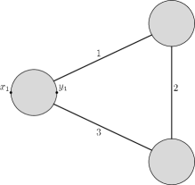
Itérons cette opération un maximum de fois. On peut toujours réduire un arbre qui recouvre le graphe direct, ayant $N(G)-1$ lignes. Le résultat de cette opération est un graphe avec un seul vertex n’ayant que des lignes de tadpole et ayant le genre du graphe initial: la rosette associée au graphe. La rosette a une racine correspondant au vertex $\bar{v}$. De plus, la rosette a un ordre cyclique, trigonométrique direct. Nous avons besoin de cet ordre cyclique pour préciser l’ordre des points sur la rosette. Un exemple est donné dans la figure 6.3. Les lignes conservent leurs orientations et pour les graphes orientables elles sortent des points pairs et entrent dans les points impairs.

Figure 6.3: Rosette avec racine explicitée

Dans l’annexe D nous prouvons que cette opération reproduit la forme du facteur d’oscillation d’un graphe. Par conséquent, pour évaluer un terme de la somme 6.11 il suffit de regarder la rosette associée à un graphe et de lui associer le facteur:

$$-\sum_{i,j}\omega^{\bar{v}}(i,j)\varepsilon_{\ell i}\varepsilon_{\ell j}$$ (6.12)

La seconde opération topologique est la réduction d’une ligne d’arbre dans le graphe dual. Cette opération efface la ligne dans le graphe direct. Le genre du graphe (direct et dual) ne change pas sous cette opération. En itérant cette operation maximalement, nous réduisons $F(G)-1$ lignes d’un arbre dans le graphe dual. Nous aboutissons à un graphe ayant $N(G)-1$ lignes d’un arbre $T(G)$ dans le graphe direct réduites et $F(G)-1$ lignes d’un arbre ${\cal T}(G)$ du graphe dual réduites. Ce graphe est une rosette avec une seule face, appelé superrosette. Son dual est aussi une superrosette. Un exemple est présenté dans la figure 6.4.

Figure 6.4: Une superrosette

Cette opération va simplement effacer les lignes et colonnes correspondantes aux lignes du graphe dual réduites de la matrice $B^{\prime}$.

La troisième opération topologique est la réduction du genre d’une rosette. Un croisement naturel est un croisement des deux lignes sur une rosette tel que le point final de la première ligne succède au point initial de la deuxième sur la rosette. De telles lignes ont une face interne commune. Si une rosette a des croisements, elle aura certainement des croisements naturels. Les lignes $2-5$ et $4-8$ dans la figure 6.3 sont un exemple de croisement naturel.

La réduction du genre efface les lignes d’un croisement naturel et permute les points survolés par les deux lignes, comme dans la figure 6.5. On appelle cette opération le troisième mouvement de Filk. Elle diminue le nombre de lignes par $2$, recolle les faces d’une manière cohérente, et décroît le genre par $1$. En terme des variables grassmanniennes, cela correspond à apparier les deux variables des lignes d’un croisement naturel.

Figure 6.5: Troisième mouvement de Filk

A l’aide de cette troisième opération nous prouvons que

Lemma 6.2.1

Le déterminant associé à une rosette vaut

• $0$ si $F(G)$ est plus grand que $1$

• $2^{2g}$ si $F(G)=1$

Pour avoir un terme non nul il suffit donc de choisir $J$ admissible, ce qui veut dire que:

• $J$ contient un arbre ${\cal T}(G)$ dans le graphe dual,

• le complément de $J$ contient un arbre $T(G)$ dans le graphe direct

• La rosette obtenue en effaçant les lignes de $J$ et en contractant les lignes de $T(G)$ est un superrosette, donc à une seule face.

Nous avons la borne:

$$HU_{G,\bar{v}}\geq\sum_{Jadmissible}\left(\frac{2}{\Omega}\right)^{2g-k_{J}}\prod_{\ell\in J}t_{\ell}\;,$$ (6.13)

avec $k_{J}=|J|-F(G)+1$.

Les termes dominants sont ceux avec $|J|$ minimal, donc ceux pour lesquels $J$ est un arbre ${\cal T}(G)$ dans le graphe dual et l’on a:

$$HU_{G,\bar{v}}\geq\left(\frac{2}{\Omega}\right)^{2g}\sum_{{\cal T}(G)}\prod_{\ell\in{\cal T}(G)}t_{\ell}\;.$$ (6.14)

Nous allons utiliser cette borne pour évaluer le degré de divergence d’un graphe. Nous nous plaçons à attribution d’échelle fixée $0\leq t_{1}\leq t_{2}\dots\leq t_{L(G)}$. Nous changeons de variable dans $t_{1}=\lambda^{2}$, $t_{i}=\lambda^{2}x_{i}$. La divergence ou convergence du graphe est gouvernée par la nature de l’intégrale sur $\lambda$:

$${\cal A}\leq\int_{0}d\lambda\lambda^{2L(G)-1+D[F(G)-1]}\sim\int_{0}d\lambda\lambda^{-1}\lambda^{8g(G)+N_{e}(G)-4}\,,$$ (6.15)

où nous avons utilisé $N(G)-L(G)+F(G)=2-2g(G)$ et $2L(G)=4N(G)-N_{e}(G)$. Nous voyons tout de suite que l’intégrale au-dessus est certainement convergente si le graphe a plus de quatre pattes externes ou s’il est non-planaire. Par des traitements similaires nous pouvons conclure qu’un graphe est convergent aussi s’il a plus d’une face brisée.

Dans ce chapitre nous avons introduit la représentation paramétrique dans la TCNC. La continuation naturelle de notre traitement est de procéder à la régularisation et renormalisation dimensionnelle de notre modèle. Ce programme sera achevé dans le chapitre suivant.

Une autre direction de recherche est d’approfondir les nouveaux polynômes hyperboliques introduits dans notre travail. Les bi-arbres, ensembles des lignes formés d’un arbre dans le graphe direct et un arbre dans le graphe dual, sont la généralisation des arbres de Symanzick pour les TCNC sur le plan de Moyal. Leur étude semble être nécessaire pour la construction finale du modèle. Nous pensons que des théorèmes généralisant celles du type "tree-matrix" (voir [67]) pourront être établis.

La dualité de Langmann-Szabo se traduit au niveau des polynômes par une symétrie $\Omega\to\Omega^{-1}$. Cette propriété sera exploitée pour établir la liste complète des termes des polynômes.

Chapitre 7 Régularisation dimensionnelle

Dans le chapitre précédent nous avons obtenu la représentation paramétrique du modèle $\Phi^{\star 4}_{4}$. Dans ce chapitre nous allons appliquer cette représentation afin d’achever sa régularisation et la renormalisation dimensionnelle (RRD).

Une raison pour s’intéresser à la régularisation dimensionnelle est qu’elle est le seul schéma d’extraction des singularités dans la théorie des champs qui respecte les invariances de jauge. Il est vrai que l’on ne possède pas pour l’instant une théorie de jauge non commutative vulcanisée bien établie; néanmoins, une fois une telle théorie obtenue, il sera naturel de la renormaliser à l’aide des techniques introduites dans ce chapitre.

Il y a une deuxième raison d’examiner la RRD. La localité des contre-termes dans les théories commutatives répose sur des propriétés de factorisation des polynômes de Symanzik. Ces propriétés sont faciles à prouver à partir de la forme explicite des polynômes. La moyalité, dans notre cas, va reposer sur le même type de propriétés. Cette fois-ci la factorisation est bien plus difficile à prouver. Nous devons nous appuyer sur des manipulations nontriviales au niveau des variables de Grassmann.

Une fois la factorisation des amplitudes établie il est possible de réformuler la RRD dans le langage des algèbres de Connes-Kreimer. L’approche algébrique à la renormalisation peut ensuite être exploitée pour formuler et résoudre des nouvelles classes de problèmes de Hilbert.

Pour effectuer la RRD nous devons combiner les techniques classiques du cas commutatif avec les résultats nouveaux charactéristiques du monde non commutatif. La principale différence par rapport au cas commutatif vient du fait que nous avons une nouvelle catégorie de graphes primitivement divergents. La preuve de la méromorphie et l’extraction des pôles, par contre, est formellement identique dans les cas commutatif et non commutatif.

Comme déjà mentionné auparavant, nous avons besoin d’une amélioration par rapport aux résultats obtenus dans le chapitre précédent. En effet, l’amélioration du comptage des puissances d’un graphe dans le nombre de faces brisées n’est apparente qu’en utilisant le deuxième polynôme. Pour un sous-graphe d’un grand graphe, par contre, nous avons une amélioration déjà au niveau du premier polynôme. Pour la mettre en évidence l’on doit utiliser des termes dominants supplémentaires de $G$, avec un scaling global en $t_{G}^{F(G)+2g(G)-1}$, mais avec un scaling dans les variables de $S$ en $t_{S}^{F(S)-2}$ si $B(S)\geq 2$. L’existence de tels termes sera prouvée par la suite.

L’extraction des singularités dans la RRD se fait de la manière suivante: Nous introduisons des secteurs de Hepp. Les intégrales sur les paramètres de Hepp des sous-graphes $S$ du graphe $G$ qui ne sont pas primitivement divergents convergent. Pour les $S$ primitivement divergents nous obtenons des singularités explicites que nous extrayons.

Pour prouver techniquement que les intégrales correspondantes aux sousgraphes planaires avec plus d’une face brisée sont convergentes nous avons besoin de nous appuyer sur certains termes dominants du première polynôme. Ces termes existent, mais ils ne sont pas parmi ceux explicités dans le chapitre précédent.

7.1 Les termes dominants supplémentaires

Les nouveaux termes sont associés à des ensembles $I$ et $J$ particuliers. Pour les spécifier nous devons introduire quelques définitions.

Appelons "ligne de genre" une ligne qui fait partie d’un croisement naturel. Soit $S$ un sous-graphe planaire de $G$ avec plus d’une face brisée. Nous appelons $\tilde{\ell}$ la ligne de $G$ qui brise la face de $S$.

Si l’on réduit $S$ à une rosette il existe une ligne de boucle $\ell_{2}\in S$ qui soit croise $\tilde{\ell}$, soit la survole. Cette ligne $\ell_{2}$ sépare deux faces brisées de $S$.

Definition 7.1.1

Soit $J_{0}$ un sous-ensemble de lignes internes du graphe $G$. $J_{0}$ est appelé pseudo-admissible si:

• Son complément est l’union d’un arbre $T(G)$ de $G$ et $\ell_{2}$,

• Ni $\tilde{\ell}$ ni $\ell_{2}$ n’appartienent pas à $T(G)$,

Soit $I_{0}=\{\ell_{1}\ldots\ell_{L}\}-\tilde{\ell}\equiv I-\tilde{\ell}$. Nous avons $|I_{0}|=L(G)-1$ et $|J_{0}|=L(G)-N(G)=F(G)-2+2g(G)$.

Theorem 7.1.1

Le pfaffien associé à $I_{0}$ et $J_{0}$ est

$$n_{I_{0},J_{0}}^{2} = 4,\mbox{ si $\tilde{\ell}$ est une ligne de genre de $G$}$$

$$= 16,\mbox{ si $\tilde{\ell}$ n'est pas une ligne de genre de $G$.}$$

Nous utilisons le lemme précédent de la façon suivante: Choisissons pour $T(G)$ un arbre, qui restreint à $S$ est sous-arbre . Un terme correspondant à un pfaffien du haut a un préfacteur de la forme:

$$t_{\tilde{\ell}}\prod_{\ell\notin T(G)\text{ et }\ell\neq\ell_{2}}t_{\ell}\,.$$ (7.1)

Le degré global dans les variables $t_{G}$ est $F(G)+2g(G)-1$, donc il s’agit bien d’un terme dominant pour le graphe $G$.

Le degré dans les variables $t_{S}$ est $L(S)-(N(S)-1)-1=L(S)-N(S)=F(S)-2$, car $S$ est planaire. Par conséquent, sous rescaling de tous les $t_{S}$ par $x_{i}^{2}$ le degré minimal de $x_{i}$ est au plus $x_{i}^{2[L(S)-N(S)]}$.

7.2 Factorisation

Dans la représentation paramétrique la localité des contre-termes dans la théorie commutative se traduit par les propriétés de factorisation des polynômes. Au niveau du premier polynôme, présenté dans l’équation (6.2):

$$U_{G}=\sum_{T}\prod_{l\not\in T}\alpha_{l}\ ,$$ (7.2)

cela se traduit par la propriété suivante: Soit $S$ un sous-graphe primitivement divergent de $G$ (un sous-graphe à deux ou à quatre pattes externes) et $G/S$ le graphe $G$ où le sous-graphe $S$ a été réduit à un point. Le polynôme des $G$ se sépare dans la somme des deux contributions suivantes:

$$U_{G}=\sum_{T,T|_{S}\text{ arbre en }S}\prod_{l\not\in T}\alpha_{l}+\sum_{T,T|_{S}\text{ n'est pas un arbre en }S}\prod_{l\not\in T}\alpha_{l}\,,$$ (7.3)

Sous un rescaling de tous les paramètres $\alpha_{S}\mapsto\rho^{2}\alpha_{S}$ l’ordre dominant en $\rho$ du polynôme $U_{G}$ est donné par la première contribution du haut, $U_{G}^{1}$:

$$U_{G}^{1} = \rho^{2[L(S)-N(S)+1]}\sum_{T_{1}\text{ arbre en }S}\prod_{l\not\in T_{1}}\alpha_{l}\sum_{T_{2},T_{2}\text{ arbre en }G/S}\prod_{l\not\in T_{2}}\alpha_{l}$$ (7.4)

$$= \rho^{2[L(S)-N(S)+1]}U_{S}U_{G/S}\,.$$

Nous allons prouver une propriété similaire pour les polynômes des TCNC. Comme la forme de ces polynômes est beaucoup plus complexe que la forme des polynômes de Simanzik, la preuve de cette factorisation est très technique. En effet, pour prouver la factorisation nous devons retourner à l’expression des polynômes comme déterminants et ensuite prouver que ces déterminants se factorisent comme des produits des deux autres déterminants.

Soit $S$ un sous-graphe primitivement divergent de $G$. $S$ est donc planaire avec une seule face brisée et à deux ou quatre pattes externes. $G/S$ est le graphe $G$ où $S$ a été réduit à un vertex de Moyal (voir figures 7.1, et 7.2).

Figure 7.1: Un graphe avec un sous-graphe primitivement divergent ($\ell_{4},\ell_{5}$ $\ell_{6}$)

Figure 7.2: Le graphe $G/S$

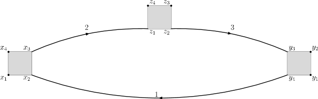
Nous notons par $l(\rho)$ les termes dominants en $\rho$ dans la zone ultraviolette. Dans l’appendice E nous prouvons les deux affirmations suivantes:

Theorem 7.2.1

Sous le rescaling

$$t_{\alpha}\mapsto\rho^{2}t_{\alpha}$$ (7.5)

des paramètres correspondant à un sous-graphe divergent $S$ d’un graphe $G$, le premier polynôme factorise comme:

$$HU^{l(\rho)}_{G,\bar{V}}=HU^{l(\rho)}_{S,\bar{V}_{S}}HU_{G/S,\bar{V}}\;.$$ (7.6)

Pour la partie exponentielle on a le résultat:

Proposition 7.2.2

Sous le rescaling $t_{\alpha}\mapsto\rho^{2}t_{\alpha}$ des paramètres du sous-graphe $S$ nous avons:

$$\frac{HV_{G}}{HU_{G}}\Big{|}_{\rho=0}=\frac{HV_{G/S}}{HU_{G/S}}\,.$$ (7.7)

Mis ensemble ces deux résultats donnent la factorisation des intégrants des amplitudes:

$$\frac{e^{-\frac{HV_{G}(\rho)}{HU_{G}(\rho)}}}{HU_{G}(\rho)^{D/2}}=\frac{1}{[HU^{l(\rho)}_{S}]^{D/2}}(1+\rho^{2}{\cal O}_{S})\frac{e^{-\frac{HV_{G/S}}{HU_{G/S}}}}{HU_{G/S}^{D/2}}\,.$$ (7.8)

Pour la fonction à deux points nous prouvons en plus que l’opérateur ${\cal O}_{S}$ correspond à une renormalisation de masse et de fonction d’onde.

7.3 Méromorphie

Nous présentons ci-dessous en détail la preuve de la méromorphie des amplitudes de Feynman en TCNC. La procédure de soustraction est similaire à celle des théories commutatives et nous n’insistons pas sur ces détails ici.

L’amplitude d’un graphe de Feynman s’écrit:

$${\cal A}_{G,{\bar{V}}}(x_{e},\;p_{\bar{V}},D)=\left(\frac{\tilde{\Omega}}{2^{\frac{D}{2}-1}}\right)^{L}\int_{0}^{1}\prod_{\ell=1}^{L}dt_{\ell}(1-t_{\ell}^{2})^{\frac{D}{2}-1}\frac{e^{-\frac{HV_{G,\bar{V}}(t_{\ell},x_{e},p_{\bar{v}})}{HU_{G,\bar{v}}(t)}}}{HU_{G,\bar{V}}(t)^{D/2}}\,.$$ (7.9)

Nous analysons seulement les graphes connexes avec au moins deux pattes externes. Nous prolongeons cette expression dans le plan complexe. On définit un secteur de Hepp $\sigma$ comme:

$$0\leq t_{1}\leq\ldots\leq t_{L}\,,$$ (7.10)

et nous effectuons le changement de variables adapté:

$$t_{\ell}=\prod_{j=\ell}^{L}x_{j}^{2},\ \ell=1,\ldots,L.$$ (7.11)

Soit $G_{i}$ le sous-graphe composé par les lignes $t_{1}$ à $t_{i}$. On note $L(G_{i})=i$ le nombre des lignes de $G_{i}$, $g(G_{i})$ son genre, $F(G_{i})$ son nombre de faces, et ainsi de suite. L’amplitude est:

$${\cal A}_{G,\bar{V}}= \Big{(}\frac{\tilde{\Omega}}{2^{(D-4)/2}}\Big{)}^{L}\int_{0}^{1}\prod_{i=1}^{L}\left(1-(\prod_{j=i}^{L}x_{j}^{2})^{2}\right)^{\frac{D}{2}-1}dx_{i}$$ (7.12)

$$\prod_{i=1}^{L}x_{i}^{2L(G_{i})-1}\frac{e^{-\frac{HV_{G,\bar{V}}(x^{2})}{HU_{G,\bar{V}}(x^{2})}}}{HU_{G,\bar{V}}(x^{2})}\,.$$

Dans l’équation ci-dessus nous factorisons dans $HU_{G,\bar{V}}$ le monôme avec le plus petit degré dans chaque variable $x_{i}$:

$${\cal A}_{G,{\bar{V}}}(x_{e},\;p_{\bar{v}})= \left(\frac{\tilde{\Omega}}{2^{\frac{D}{2}}}\right)^{L}\int_{0}^{1}\prod_{\ell=1}^{L}dx_{\ell}\left(1-(\prod_{j=\ell}^{L}x_{j}^{2})^{2}\right)^{\frac{D}{2}-1}$$ (7.13)

$$x_{i}^{2L(G_{i})-1-Db^{\prime}(G_{i})}\frac{e^{-\frac{HV_{G,\bar{V}}}{HU_{G,\bar{V}}}}}{(as^{b}+F(x^{2}))^{\frac{D}{2}}}.$$

Le dernier terme ci-dessus est toujours borné par une constante. Des divergences ne peuvent apparaître que dans la région $x_{i}$ proche de $0$. Nous retrouvons, comme auparavant, que cette théorie n’a pas de divergences infrarouges même à masse zéro. Le nombre $b^{\prime}(G_{i})$ est fixé par la topologie du graphe $G_{i}$. Il vaut:

$$b^{\prime}(G_{i})=\begin{cases}{\displaystyle\leq L(G_{i})-[n(G_{i})-1]-2g(G_{i})}&\text{si }g(G_{i})>0\vspace{.3cm}\\ {\displaystyle\leq L(G_{i})-n(G_{i})}&\text{si }g(G_{i})=0\text{ et }B(G_{i})>1\vspace{.3cm}\\ {\displaystyle=L(G_{i})-[n(G_{i})-1]}&\text{si }g(G_{i})=0\text{ et }B(G_{i})=1\\ \end{cases}.$$

Pour prouver la première et la dernière ligne nous devons analyser des termes dominants du $HU_{G}$ avec $I=\{1\ldots L\}$ et $J$ admissible en $G$, tel que l’arbre $T(G)$, inclut dans l’ensemble complémentaire de $J$, est sous-arbre en $G_{i}$.

Pour la deuxième ligne nous devons choisir $I=\{1\ldots L\}-\tilde{\ell}$ et $J$ pseudo-admissible, comme dans la section 7.1.

Nous pouvons conclure que $b^{\prime}(G_{i})$ est au plus $L(G_{i})-n(G_{i})+1$ et qu’il prend cette valeur si et seulement si $g(G_{i})=0$ et $B(G_{i})=1$. Par conséquent, la convergence dans le régime UV ($x_{i}\to 0$) est assurée si:

$$\Re[2L(G_{i})-Db^{\prime}(G_{i})]>0,\ i=1\ldots L\,.$$ (7.14)

Comme

$$\Re[2L(G_{i})-Db^{\prime}(G_{i})]>\Re\Big{(}2L(G_{i})-D[L(G_{i})-n(G_{i})+1]\Big{)}\,,$$ (7.15)

on a toujours convergence pourvu que:

$$\Re D<2\leq\frac{4n(G_{i})-N(G_{i})}{n(G_{i})-N(G_{i})/2+1}\leq\frac{2L(G_{i})}{L(G_{i})-n(G_{i})+1}\,.$$ (7.16)

avec $N_{e}(G_{i})$ le nombre des points externes de $G_{i}$ . Donc ${\cal A}_{G,\bar{V}}(D)$ est analytique dans la bande

$${\cal D}^{\sigma}=\{D\,|\,0<\Re\,D<2\}.$$ (7.17)

On prolonge maintenant ${\cal A}$ comme fonction de $D$ pour $2\leq\Re D\leq 4$. Pourvu que:

• $g(G_{i})>0$

• $g(G_{i})=0$ and $B(G_{i})>1$

• $N(G_{i})>4$   ,

la bande d’analyticité est immédiatement prolongée à:

$${\cal D}^{\sigma}=\{D\,|\,0<\Re\,D<4+\varepsilon_{G}\}.$$ (7.18)

pour $\varepsilon_{G}$ un petit nombre positif dépendent du graphe.

En effet, dans les premiers deux cas on a $b^{\prime}(G_{i})\leq L(G_{i})-n(G_{i})$ donc l’intégrale sur $x_{i}$ converge pour:

$$\Re D\leq 4<\frac{4n(G_{i})-N(G_{i})}{n(G_{i})-N(G_{i})/2}=\frac{2L(G_{i})}{L(G_{i})-n(G_{i})}\,,$$ (7.19)

et dans le troisième cas, comme $N(G_{i})>4$, l’intégrale sur $x_{i}$ converge pour:

$$\Re D\leq 4<\frac{4n(G_{i})-N(G_{i})}{n(G_{i})-N(G_{i})/2+1}=\frac{2L(G_{i})}{L(G_{i})-n(G_{i})+1}\,.$$ (7.20)

Seuls les sous-graphes planaires avec une seule face brisée avec deux ou quatre points présentent des divergences UV dans la bande $2,4+\varepsilon$. Ils sont appelés primitivement divergents. Soit $S$ un sous-graphe primitivement divergent. On note son paramètre de Hepp $\rho$. En utilisant l’équation (7.8), sa contribution à l’amplitude est:

$${\cal A}^{\rho}_{G,\bar{V}_{G}}\sim\int_{0}d\rho\rho^{2L(S)-1-D[L(S)-n(S)+1]}\frac{1}{HU^{l}_{S,\bar{V}_{S}}|_{\rho=1}}(1+\rho^{2}{\cal O}_{S})\frac{e^{-\frac{HV_{G/S}}{HU_{G/S}}}}{HU_{G/S}}\,.$$

L’intégrale sur $\rho$ est un opérateur méromorphique en $D$ avec la partie divergente donnée par:

$$\frac{r_{1}}{2L(S)-D[L(S)-n(S)+1]}+\frac{r_{2}}{2L(S)-D[L(S)-n(S)+1]+2}{\cal O}_{S}\,.$$

Nous avons un pôle isolé à $D=4$ si $S$ a quatre points. Si $S$ a deux points, nous avons deux pôles, l’un à $D=4-2/N(S)$ et l’autre à $D=4$. Comme toutes les singularités sont de ce type, nous avons prouve que ${\cal A}_{G}$ est méromorphe dans la bande:

$${\cal D}^{\sigma}=\{D\,|\,0<\Re\,D<4+\varepsilon_{G}\}.$$ (7.21)

$\Box$

Dans notre étude nous avons prouvé la factorisation des amplitudes de Feynman des TCNC. Nous avons réussi à prouver que les amplitudes sont des fonctions holomorphes dans le plan complexe (la généralisation de notre preuve pour la bande $0,4$ pour tout le plan complexe étant triviale). Une fois la structure des singularités établie nous avons pu les extraire à l’aide des opérateurs de Taylor (voir appendice E).

Pour le futur, une voie de recherche sera de reprendre les mêmes procédures pour une théorie de jauge vulcanisée. Comme nous ne disposons pas pour l’instant d’une telle théorie, nous ne pouvons pas démarrer un tel programme pour l’instant.

Une autre voie de recherche qui devrait aboutir à une réponse est de trouver lequel des traitements que nous avons effectués peut se généraliser pour d’autres variétés non commutatives.

Une autre question très intéressante est d’essayer d’établir un nombre de conditions nécessaires et suffisantes pour que les amplitudes de Feynman se factorisent. Si nous disposons d’une telle caractérisation, nous pourrons nous prononcer sur la question de la renormalisabilité pour des théories des champs plus génériques.

Chapitre 8 Le représentation de Mellin complète

En s’appuyant sur la représentation paramétrique des TCNC introduite dans [39, 40], nous allons maintenant introduire la représentation de Mellin Complète (CM) du modèle $\Phi^{\star 4}_{4}$. Cette représentation des amplitudes de Feynman est la plus compacte connue. De plus, elle est un nouveau point de départ pour la renormalisation et pour l’étude des comportements asymptotiques des amplitudes sous rescaling arbitraire des invariants externes.

Dans les théories commutatives le problème du développement asymptotique est formulé de la manière suivante. Etant donnée une amplitude de Feynman nous rescalons l’un de ses invariants externes par un paramètre $\alpha$. Nous cherchons à exprimer l’amplitude comme série asymptotique de puissances et puissances du logarithme de $\alpha$. La représentation de Mellin nous fournit ce développement dans certains cas.

Une propriété des polynômes de la représentation paramétrique requise pour pouvoir prouver l’existence d’un développement asymptotique est la propriété FINE. Un polynôme est appelé FINE s’il se factorise dans tout secteur de Hepp. Pour les polynômes FINE la transformation de Mellin inverse, qui nous donne l’amplitude en fonction de $\alpha$, a une structure méromorphe et ses résidus nous donne l’expansion asymptotique.

Si un polynôme n’est pas FINE, nous pouvons le décomposer dans plusieurs morceaux, chacun avec la propriété FINE. Nous pouvons ensuite associer un paramètre de Mellin à tout sous-polynôme FINE. Si nous poussons ce raisonnement à ses limites, nous pouvons associer un paramètre de Mellin à tout monôme. Cette représentation est appelée "Mellin Complète" (CM).

De plus, dans le cadre de cette représentation, nous pouvons intégrer les paramètres de Schwinger et nous pouvons reformuler la renormalisation comme l’étude des déplacements des pieds des contours d’intégration des variables de Mellin dans des cellules du plan complexe. Cela nous permet de traiter au même niveau les amplitudes divergentes et convergentes dans l’ultraviolet.

A l’aide de la représentation CM nous prouvons le résultat suivant. Soit une amplitude de Feynman $G(s_{k})$ écrite en fonction des ses invariants $s_{k}$ (on inclut aussi les masses des particules). Soit un régime asymptotique défini par:

$$s_{k}\rightarrow\alpha^{a_{k}}{s}_{k},$$ (8.1)

avec $a_{k}$ positif, négatif, ou nul.

Nous laissons $\alpha$ tendre vers l’infini. $G(s_{k})$ a un développement asymptotique comme fonction de $\alpha$ du type:

$$G(\alpha;s_{k})=\sum_{p=p_{\text{max}}}^{-\infty}\sum_{q=0}^{q_{\text{max}}(p)}G_{pq}(s_{k})\alpha^{p}\ln^{q}\alpha,$$ (8.2)

où $p$ est un nombre rationnel ($p_{max}$ son maximum) et $q$, à $p$ donné, est un nombre naturel.

Notre but final est de retrouver un tel résultat pour TCNC. Nous allons nous concentrer par la suite sur le début, soit l’introduction de la CM pour TCNC. Nous trouvons une structure distributionnelle plus compliquée que dans le cas commutatif, mais nous obtenons un premier résultat, celui de la méromorphie des amplitudes de Feynman.

8.1 La représentation CM dans la TCNC

Pour toute fonction $f(u)$, dérivable par morceaux pour $u>0$, si l’intégrale

$$g(x)=\int_{0}^{\infty}du\,u^{-x-1}f(u)$$ (8.3)

est absolument convergente pour $\alpha<\Re x<\beta$, alors pour $\alpha<\sigma<\beta$

$$f(u)=\frac{1}{2\pi i}\int_{\sigma-i\infty}^{\sigma+i\infty}dx\,g(x)\,u^{x}.$$ (8.4)

La fonction $g$ s’appelle la transformée de Mellin de $f$.

Pour $f(u)=e^{-u}$, et $u=HV_{k}/HU$, la transformée de Mellin inverse est:

$$e^{-HV_{k}/HU}=\int_{\tau_{k}}\Gamma(-y_{k})\left(\frac{HV_{k}}{HU}\right)^{y_{k}},$$ (8.5)

où $\int_{\tau_{k}}$ est une notation abrégée pour $\int_{-\infty}^{+\infty}\frac{d(\Im y_{k})}{2\pi}$, et $\Re y_{k}$ est fixé à $\tau_{k}<0$.

Pour tout $u$ positif, en choissant $x$ avec $\Re x<0$, tel que $0<\Re x+u$, nous avons l’égalité suivante:

$$\Gamma(u)\left(A+B\right)^{-u}=\int_{-\infty}^{\infty}\frac{d(\text{Im }x)}{2\pi}\Gamma(-x)A^{x}\Gamma(x+u)B^{-x-u}.$$ (8.6)

Nous prenons $A\equiv HU_{1}$ et $B\equiv HU_{2}+HU_{3}+\cdots$ et nous utilisons itérativement l’égalité ci-dessus pour $u=\sum_{k}y_{k}+D/2$, pour obtenir:

$$\Gamma\left(\sum_{k}y_{k}+\frac{D}{2}\right)HU^{-\sum_{k}y_{k}-\frac{D}{2}}=\int_{\sigma}\prod_{j}\Gamma(-x_{j})HU_{j}^{x_{j}},$$ (8.7)

avec $\Re x_{j}=\sigma_{j}<0$, $\Re\left(\sum_{k}y_{k}+\frac{D}{2}\right)=\sum_{k}\tau_{k}+\frac{D}{2}>0$, et $\int_{\sigma}$ veut dire $\int_{-\infty}^{+\infty}\prod_{j}\frac{d(\Im x_{j})}{2\pi}$ avec $\sum_{j}x_{j}+\sum_{k}y_{k}=-\frac{D}{2}$.

Pour utiliser les deux transformations présentées ci-dessus nous devons séparer les polynômes hyperboliques dans des sommes des monômes. Pour cela, nous commençons par l’expression du premier polynôme:

$$HU_{{\cal G},{\bar{V}}}(t) = \sum_{{K_{U}}=I\cup J,\ n+|{K_{U}}|\;{\rm impaire}}s^{2g-k_{{K_{U}}}}\ n_{{K_{U}}}^{2}\prod_{\ell\not\in I}t_{\ell}\prod_{\ell^{\prime}\in J}t_{\ell^{\prime}}\$$ (8.8)

$$= \sum_{{K_{U}}}a_{K_{U}}\prod_{\ell}t_{\ell}^{u_{\ell{K_{U}}}}\equiv\sum_{K_{U}}HU_{K_{U}}.$$

avec:

• $I$ sous-ensemble des premiers $L$ indices avec son cardinal $|I|$, $J$ sous-ensemble des $L$ indices suivants de cardinal $|J|$,

• $B$ est la matrice antisymétrique restante,

• $n_{{K_{U}}}=\mathrm{Pf}(B_{\widehat{{K_{U}}}})$ le pfaffien de $B$ avec les index de ${K_{U}}=I\cup J$ omis,

• $k_{{K_{U}}}$ est $|{K_{U}}|-L(G)-F(G)+1$,

• $a_{K_{U}}=s^{2g-k_{{K_{U}}}}n_{{K_{U}}}^{2}$, $s=\Omega^{-1}$,

  $$u_{\ell{K_{U}}}=\left\{\begin{array}[]{ll}0&\mbox{ si }\ell\in I\mbox{ et }\ell\notin J\\ 1&\mbox{ si }(\ell\notin I\mbox{ et }\ell\notin J)\mbox{ ou }(\ell\in I\mbox{ et }\ell\in J)\\ 2&\mbox{ si }\ell\notin I\mbox{ et }\ell\in J\end{array}\right..$$ (8.9)

Le second polynôme $HV$ se décompose en partie réelle $HV^{\cal R}$ et imaginaire $HV^{\cal I}$. En plus des ensembles $I$ et $J$ du haut, nous introduisons une ligne particulière $\tau\notin I$, analogue d’une coupure d’un arbre en deux. Définissons $\mathrm{Pf}(B_{\hat{{K_{V}}}\hat{\tau}})$ le pfaffien de la matrice obtenue de $B$ en effaçant les lignes et les colonnes dans $I$, $J$ et $\tau$. De plus, nous définissons $\varepsilon_{I,\tau}$ la signature de la permutation:

$$1,\dotsc,d\rightarrow 1,\dotsc,\hat{i_{1}},\dotsc,\hat{i_{|I|}},\dotsc,\hat{i_{\tau}},\dotsc,d,i_{\tau},i_{|I|}\dotsc,i_{1}\,.$$ (8.10)

avec $d=2L(G)+N(G)-1$. Alors:

$$HV^{\cal R}_{{\cal G},{\bar{V}}} = \sum_{{K_{V}}=I\cup J}\prod_{\ell\notin I}t_{\ell}\prod_{\ell^{\prime}\in J}t_{\ell^{\prime}}\Big{[}\sum_{e_{1}}x_{e_{1}}\sum_{\tau\notin{K_{V}}}P_{e_{1}\tau}\varepsilon_{{K_{V}}\tau}\mathrm{Pf}(B_{\hat{{K_{V}}}\hat{\tau}})\Big{]}^{2}\,.$$ (8.11)

$$= \sum_{K_{V}}s^{\cal R}_{K_{V}}\left(\prod_{\ell=1}^{L}t_{\ell}^{v_{\ell{K_{V}}}}\right)\equiv\sum_{K_{V}}HV_{K_{V}}^{\cal R}$$

avec

$$s_{K_{V}}^{\cal R}=\left(\sum_{e}x_{e}\sum_{\tau\notin{K_{V}}}P_{e\tau}\varepsilon_{{K_{V}}\tau}\mathrm{Pf}(B_{\hat{{K_{V}}}\hat{\tau}})\right)^{2}$$ (8.12)

et $v_{\ell{K_{V}}}$ sont donnés par la même formule que $u_{\ell K_{U}}$.

La partie imaginaire fait intervenir de paires des lignes $\tau,\tau^{\prime}$ et une signature correspondante (détaillée en [39]):

$$HV_{{\cal G},\bar{V}}^{\cal I} = \sum_{{K_{V}}=I\cup J}\prod_{\ell\notin I}t_{\ell}\prod_{\ell^{\prime}\in J}t_{\ell^{\prime}}$$ (8.13)

$$\varepsilon_{K_{V}}\mathrm{Pf}(B_{\hat{{K_{V}}}})\Big{[}\sum_{e_{1},e_{2}}\Big{(}\sum_{\tau\tau^{\prime}}P_{e_{1}\tau}\varepsilon_{{K_{V}}\tau\tau^{\prime}}\mathrm{Pf}(B_{\hat{{K_{V}}}\hat{\tau}\hat{\tau^{\prime}}})P_{e_{2}\tau^{\prime}}\Big{)}x_{e_{1}}\wedge x_{e_{2}}\Big{]}\,.$$

$$= \sum_{K_{V}}s^{\cal I}_{K_{V}}\left(\prod_{\ell=1}^{L}t_{\ell}^{v_{\ell{K_{V}}}}\right)\equiv\sum_{K_{V}}HV_{K_{V}}^{\cal I}$$

avec:

$$s_{K_{V}}^{\cal I}=\varepsilon_{K_{V}}\mathrm{Pf}(B_{\hat{{K_{V}}}})\left(\sum_{e,e^{\prime}}(\sum_{\tau,\tau^{\prime}}P_{e\tau}\varepsilon_{{K_{V}}\tau\tau^{\prime}}\mathrm{Pf}(B_{\hat{{K_{V}}}\hat{\tau}\hat{\tau^{\prime}}})P_{e^{\prime}\tau^{\prime}})x_{e}\wedge x_{e^{\prime}}\right).$$ (8.14)

Les principales différences entre la TCNC et la TCC sont:

• la présence des constantes $a_{j}$ dans $HU$,

• la partie imaginaire $i\,HV^{\cal I}$ de $HV$,

• Le fait que $u_{\ell j}$ et $v_{\ell k}$ peuvent prendre la valeur $2$ (pas seulement $0$ et $1$).

Pour la partie réelle $HV^{\cal R}$ de $HV$ nous utilisons l’identité:

$$e^{-HV^{\cal R}_{K_{V}}/HU}=\int_{\tau_{K_{V}}^{\cal R}}\Gamma(-y_{K_{V}}^{\cal R})\left(\frac{HV^{\cal R}_{K_{V}}}{HU}\right)^{y_{K_{V}}^{\cal R}},$$ (8.15)

qui introduit l’ensemble des paramètres de Mellin $y_{K_{V}}^{\cal R}$.

Pour la partie imaginaire une identité similaire n’est vraie qu’au sens des distributions. Nous avons, pour $HV^{\cal I}_{K_{V}}/U>0$ et $-1<\tau_{K_{V}}^{\cal I}<0$:

$$e^{-i\,HV^{\cal I}_{K_{V}}/HU}=\int_{\tau_{K_{V}}^{\cal I}}\Gamma(-y_{K_{V}}^{\cal I})\left(\frac{i\,HV^{\cal I}_{K_{V}}}{HU}\right)^{y_{K_{V}}^{\cal I}}.$$ (8.16)

Nous introduisons ainsi un autre ensemble de paramètres de Mellin $y_{K_{V}}^{\cal I}$. Le caractère distributionnel de cette égalité est l’une des principales différences avec le cas commutatif.

Pour $HU$ nous utilisons la représentation:

$$\Gamma\left(\sum_{K_{V}}y_{K_{V}}+\frac{D}{2}\right)(HU)^{-\sum_{K_{V}}(y_{K_{V}}^{\cal R}+y_{K_{V}}^{\cal I})-\frac{D}{2}}=\int_{\sigma}\prod_{K_{U}}\Gamma(-x_{K_{U}})HU_{K_{U}}^{x_{K_{U}}},$$ (8.17)

avec $y_{K_{V}}=y_{K_{V}}^{\cal R}+y_{K_{V}}^{\cal I}$.

Une amplitude générale de Feynman s’écrit comme:

$${\cal A}_{G} = {\rm K^{\prime}}\int_{\Delta}\frac{\prod_{K_{U}}a_{K_{U}}^{x_{K_{U}}}\Gamma(-x_{K_{U}})}{\Gamma(-\sum_{K_{U}}x_{K_{U}})}\left(\prod_{K_{V}}(s_{K_{V}}^{\cal R})^{y_{K_{V}}^{\cal R}}\Gamma(-y_{K_{V}}^{\cal R})\right)$$ (8.18)

$$\left(\prod_{K_{V}}(s_{K_{V}}^{\cal I})^{y_{K_{V}}^{\cal I}}\Gamma(-y_{K_{V}}^{\cal I})\right)\int_{0}^{1}\prod_{\ell=1}^{L}dt_{\ell}(1-t_{\ell}^{2})^{\frac{D}{2}-1}t_{\ell}^{\phi_{\ell}-1}$$

avec:

$$\phi_{\ell}\equiv\sum_{K_{U}}u_{\ell{K_{U}}}x_{K_{U}}+\sum_{K_{V}}(v^{\cal R}_{\ell{K_{V}}}y_{K_{V}}^{\cal R}+v^{\cal I}_{\ell{K_{V}}}y_{K_{V}}^{\cal I})+1.$$ (8.19)

Par $\int_{\Delta}$ nous entendons une intégrale sur $\frac{\text{Im }x_{K_{U}}}{2\pi i}$, $\frac{\text{Im }y_{K_{V}}^{\cal R}}{2\pi i}$ et $\frac{\text{Im }y_{K_{V}}^{\cal I}}{2\pi i}$, où $\Delta$ est le domaine convexe

$$\Delta=\left\{\sigma,\tau^{\cal R},\tau^{\cal I}\left|\begin{array}[]{l}\sigma_{K_{U}}<0;\;\tau^{\cal R}_{K_{V}}<0;\;-1<\tau^{\cal I}_{K_{V}}<0;\\ \sum_{K_{U}}x_{K_{U}}+\sum_{K_{V}}(y_{K_{V}}^{\cal R}+y_{K_{V}}^{\cal I})=-\frac{D}{2};\\ \forall\ell,\;\text{Re }\phi_{\ell}\equiv\sum_{K_{U}}u_{\ell{K_{U}}}\sigma_{K_{U}}\\ +\sum_{K_{V}}(v^{\cal R}_{\ell{K_{V}}}\tau^{\cal R}_{K_{V}}+v^{\cal I}_{\ell{K_{V}}}\tau^{\cal I}_{K_{V}})+1>0\end{array}\right.\right\}$$ (8.20)

et $\sigma$, $\tau^{\cal R}$ et $\tau^{\cal I}$ représentent $\text{Re }x_{K_{U}}$, $\text{Re }y_{K_{V}}^{\cal R}$ et $\text{Re }y_{K_{V}}^{\cal I}$.

Les intégrales $dt_{\ell}$ peuvent être effectuées en utilisant la représentation de la fonction bêta:

$$\int_{0}^{1}\prod_{\ell=1}^{L}dt_{\ell}(1-t_{\ell}^{2})^{\frac{D}{2}-1}t_{\ell}^{\phi_{\ell}-1}=\frac{1}{2}\beta(\frac{\phi_{\ell}}{2},\frac{D}{2}).$$ (8.21)

De plus, nous avons:

$$\beta(\frac{\phi_{\ell}}{2},\frac{D}{2})=\frac{\Gamma(\frac{\phi_{\ell}}{2})\Gamma(\frac{D}{2})}{\Gamma(\frac{\phi_{\ell}+D}{2})}.$$ (8.22)

Cette représentation est convergente pour $0<\Re D<2$. Nous obtenons ainsi la représentation CM d’une amplitude de Feynman dans la TCNC:

Theorem 8.1.1

Toute amplitude de Feynman d’un graphe de $\phi^{\star 4}$ est analytique au moins dans la bande $0<\Re D<2$ où elle a la représentation CM suivante:

$${\cal A}_{\cal G} = {\rm K^{\prime}}\int_{\Delta}\frac{\prod_{K_{U}}a_{K_{U}}^{x_{K_{U}}}\Gamma(-x_{K_{U}})}{\Gamma(-\sum_{K_{U}}x_{K_{U}})}\left(\prod_{K_{V}}(s_{K_{V}}^{\cal R})^{y_{K_{V}}^{\cal R}}\Gamma(-y_{K_{V}}^{\cal R})\right)$$

$$\left(\prod_{K_{V}}(s_{K_{V}}^{\cal I})^{y_{K_{V}}^{\cal I}}\Gamma(-y_{K_{V}}^{\cal I})\right)\left(\prod_{\ell=1}^{L}\frac{\Gamma(\frac{\phi_{\ell}}{2})\Gamma(\frac{D}{2})}{2\Gamma(\frac{\phi_{\ell}+D}{2})}\right).$$

vraie en tant que distribution tempérée des invariants externes.

A partir de cette formule nous avons obtenu la continuation de la représentation CM d’une amplitude à une distribution tempérée dépendant méromorphiquement de $D$ dans tout le plan complexe.

Une fois la représentation de Mellin Complète introduite et la méromorphie prouvée nous devrons essayer de trouver les généralisations des résultats classiques obtenus à l’aide de cette représentation dans la théorie commutative. Le premier but est de reformuler la renormalisation dans le nouveau langage. Dans les théories commutatives la renormalisation est équivalente au déplacement des pieds des contours d’intégration entre différentes cellules de Mellin dans le plan complexe. La soustraction est équivalente avec le passage d’une représentation de la fonction $\Gamma(p)$ pour $0<p$ à une représentation pour $-1<p<0$. Il faut vérifier que ces soustractions sont données par des contre-termes de la forme du Lagrangien. En tenant compte des travaux présentés dans le chapitre précédent nous pensons que ce résultat suivra.

Une fois la renormalisabilité prouvée, le deuxième but est de prouver l’existence des séries asymptotiques sous un rescaling des invariants de l’amplitude. La combination de notre représentation de CM et des techniques classiques fournira très certainement ce résultat.

Chapitre 9 Conclusion

Le long de cette thèse nous avons étudié le modèle $\Phi^{\star 4}_{4}$ de plusieurs points de vue. Nous avons étudié le modèle à l’aide de diverses techniques introduites le long de nos travaux. Ainsi, nous disposons aujourd’hui pour les TCNC d’une panoplie d’outils d’analyse presque tout aussi développée que pour leurs partenaires commutatives.

Parmi les divers resultats présentés dans nos travaux, probablement le plus excitant est l’annulation de la fonction beta du modèle. Les modèles avec des flots bornés sont très cohérents du point de vue mathématique, notamment nous pouvons espérer les construire non perturbativement. Si cette caractéristique s’avère générique pour les TCNC vulcanisées elle fournira à elle seule un très fort argument en leur faveur.

Les identités de Ward que nous avons utilisées pour prouver ce résultat ont un statut très particulier. Dans les théories de champs commutatives les identités de Ward sont la conséquence de l’invariance de jauge. En considérant un modèle invariant de jauge nous devons fixer la jauge. Ensuite, si nous agissons avec une transformation de jauge infinitésimale de la même façon que dans nos travaux nous obtenons les identités de Ward.

Il semble que notre modèle initial corresponde à une action déjà fixée de jauge! Nous nous demandons donc si il existe une forme invariante de jauge associée à notre modèle. Une fois une telle invariance comprise nous devons construire une action de Yang Mills associée. Cette action sera différente des actions de Yang Mills déjà proposées par [33, 34].

Nous concluons que le sens des transformations unitaires qui intervient dans la preuve de l’annulation de la fonction bêta devrait être approfondi. Si nous considérons que les opérateurs associés aux coordonnées se transforment réellement sous les unitaires nous voyons que ces transformations correspondent aux difféomorphismes préservant l’aire. En effet, si dans une transformation:

$$x^{\prime\mu}=U^{\dagger}x^{\mu}U$$ (9.1)

nous prenons $U=e^{iH}$ avec $H$ une matrice hermétienne infinitésimale, nous voyons qu’au premier ordre en $H$ le jacobien de la transformation $x\to x^{\prime}$ est $J(x,x^{\prime})=1$. Quel est le sens physique de cette transformation? Elle apparaît naturellement dans l’étude des fluides non commutatifs (voir [10]), car les fluides sont incompressibles. Nous ne disposons pas pour l’instant d’une interprétation convaincante de ces transformations pour nos modèles.

Une direction de recherche future est la construction des modèles fermioniques non commutatifs renormalisables. Des pas dans cette direction ont été faits par Vignes-Tourneret. L’auteur a proposé une vulcanisation du modèle de Gross-Neveu engendré par un champ de fond. Le modèle est renormalisable pour tout $\Omega\neq 1$, mais la fonction bêta du modèle n’est pas nulle. Ces travaux semble suggérer que la finitude des flots n’est pas générique dans les théories vulcanisées.

Neanmoins, il existe d’autres façons de vulcaniser une théorie fermionique. Une proposition pour le modèle de Gross Neveu (et même le modèle de Yukawa non commutatif) qui ne peut pas être interprétée en terme d’un champ de fond est la suivante:

$$S=\int\bar{\psi}(\gamma^{1}\partial_{1}+\gamma^{2}\partial_{2}+\gamma^{3}\tilde{x}_{1}+\gamma^{4}\tilde{x}_{2})\psi+\lambda\bar{\psi}\star\psi\star\bar{\psi}\star\psi\;,$$ (9.2)

avec $\gamma$ des matrices de Dirac $4\times 4$. A première vue il semble étrange qu’on ait besoin des spineurs quadri-dimensionnels pour décrire un système de fermions à deux dimensions. Une telle théorie peut-elle être raisonnable?

La réponse est la suivante: la déduction historique de l’équation de Dirac part de l’équation du mouvement pour les bosons. Dirac a trouvé la bonne façon d’extraire la racine carrée du d’Alembertien:

$$\gamma^{\mu}\partial_{\mu}\gamma^{\nu}\partial_{\nu}=g^{\mu\nu}\partial_{\mu}\partial_{\nu}\;,$$ (9.3)

Dans les TCNC le bon hamiltonien libre pour les bosons à deux dimensions est:

$$H_{0}=\partial_{1}^{2}+\partial_{2}^{2}+\tilde{x}_{1}^{2}+\tilde{x}_{2}^{2}\;.$$ (9.4)

Le hamiltonien libre pour les fermions devrait être donc la racine carrée de cet opérateur, qui fait intervenir des spineurs quadri-dimensionnels. Une proposition similaire a été faite indépendament en [94]. Les auteurs introduisent un opérateur similaire en quatre dimensions (qui fait intervenir par conséquent des spineurs en seize dimensions) et l’ont utilisé pour calculer une action spectrale du type Connes-Lott d’un champ de jauge couplé à un boson de Higgs de la forme du modèle $\phi_{4}^{\star 4}$.

Nous nous proposons d’étudier par la suite cette théorie et notamment sa fonction bêta.

L’étude des théories non commutatives, et en particulier $\Phi^{\star 4}_{4}$ au niveau constructif est d’un grand intérêt. Si le modèle est construit nous disposons d’un deuxième argument de cohérence mathématique en sa faveur.

L’absence du fantôme de Landau est un bon signe qui va dans cette direction. De plus, les travaux récents de Rivasseau et Magnen [92, 93] ont abouti à la construction du modèle dans une tranche. Il nous reste néanmoins encore plusieurs points délicats à traiter. Nous avons besoin de prouver que la fonction beta est nulle constructivement, ce qui représente un travail technique non négligeable. Ensuite ces résultats devrait se combiner en une analyse constructive multi tranche de notre modèle. Il est intéressant de mentionner que la symétrie entre les faces droites et gauches intervient d’une façon cruciale dans les preuves constructives monotranche. C’est une nouvelle indication que la symétrie sous-jacente du modèle est cruciale pour sa cohérence.

Nous avons déjà mentionné les fluides non-commutatifs. Les difféomorphismes préservant l’aire intervient d’une façon très naturelle comme groupe d’invariance d’une telle théorie. Cependant nous ne savons pas encore appliquer notre groupe de renormalisation à ces théories. Cela est principalement dû aux difficultés techniques liées aux dégénérescences du propagateur. Ces singularités sont la conséquence de la structure des niveaux de Landau. A cause de l’espacement entre les niveaux nous ne pouvons pas découper le spectre du hamiltonien libre en tranches arbitrairement étroites. Nous avons testé différentes régularisations possibles, mais nous ne disposons pas pour l’instant d’une recette définitive du traitement des ces singularités.

Y-a-t il un lien entre nos travaux et la quantification de la gravitation? Nous proposons le scénario suivant:

Nous voulons traiter les opérateurs de position comme des champs quantiques et intégrer sur leurs fluctuations. En fin de compte à l’échelle de Planck l’espace temps lui même devient dynamique. Nous pouvons choisir toujours de nous placer dans un système de référence inertiel. Cela veut dire que pour toute géométrie, localement l’espace-temps tangent est plat. Nous pensons que les effets des fluctuations des opérateurs de position devraient être ressentis aussi dans ce contexte plat. Dans un tel système, en première approximation la quantification de l’espace-temps prendra la forme d’un espace de Moyal. Intégrer sur les fluctuations des opérateurs de position nous donnerait ainsi le cadre générique pour la quantification de la gravitation. Il est en plus possible que les configurations des champs avec des opérateurs de position unitairement équivalents soient sur la même section de jauge, et que nous ayons à effectuer une fixation de jauge.

Les auteurs de [49] ont traité le modèle $\Phi_{4}^{\star 4}$ avec des techniques des modèles intégrables. Dans ces travaux les auteurs ont notamment cherché une limite thermodynamique non triviale du modèle pour certaines valeurs des paramètres. L’annulation de la fonction beta au point de dualité ($\Omega=1$) indique l’existence de cette limite. Une direction de recherche future est donc la construction explicite de la fonction de partition du modèle. De plus, les conséquences de nos travaux pour des modèles de matrices généraux, mérite aussi une étude détaillée. En effet dans la base matricielle au point de dualité nous avons à faire à un modèle de matrices non identiquement distribues, sa covariance étant $\frac{1}{m+n}$. Si nous arrivons à construire explicitement la fonction de partition, nous pourrons essayer de le faire aussi pour d’autres covariances.

Une autre direction de recherche future est d’adapter nos méthodes pour des géométries non commutatives plus générales. Nous nous proposons de mener une étude de ces modèles sur des espaces-temps courbes munis de produits de Moyal adaptés. A la lumière de récents travaux sur ce sujet nous mentionnons que la Moyalité des contretermes est une caractéristique trés générale, associé aux propriétés d’associativité et de tracialité de la déformation.

Ensuite nous pourrons tester si la fonction bêta des ces modèles est nulle. La représentation paramétrique peut probablement être introduite d’une façon similaire au cas plat. Dans ces conditions la régularisation et renormalisation dimensionnelle peuvent être envisagées. Nous pouvons aussi espérer appliquer nos techniques aux variétés non commutatives plus générales, comme les sphères floues par exemple, mais nous ne savons pas encore comment vulcaniser les théories de champs sur ces variétées.

Le nouveau groupe de renormalisation que nous avons développé dans notre thèse devrait aussi trouver une application dans la reformulation du modèle standard par Connes et Chamseddine. Il est possible que la non-commutativité très simple mise en évidence par les deux auteurs (mais limitée à un espace interne) devienne plus compliquée au fur et à mesure que nous montons en énergie et envahisse l’espace-temps $\mathbb{R}^{4}$ ordinaire. Dans ces conditions le groupe de renormalisation commutatif devrait être remplacé par notre groupe de renormalisation non commutatif à partir d’une certaine échelle, entrainant une modification des flots du modèle standard.

Comme la dualité de Langmann-Szabo est la raison profonde qui tue le fantôme de Landau, on peut se poser la question de savoir si elle peut jouer un rôle similaire à la supersymétrie pour dompter les divergences UV. En effet l’idée de la supersymétrie souffre du fait que nous n’avons encore trouvé aucun partenaire supersymétrique. Si dans des expériences futures nous trouvons de tels partenaires, ils seront de toute façon de plusieurs ordres de grandeur plus lourds, ce qui devrait être expliqué. Les partenaires des électrons sont déjà bien plus lourds que ceux-ci, mais la situation est bien pire pour les neutrinos. Cet écart énorme a du mal à s’interpréter avec les théories actuelles. Il est donc raisonnable de chercher des alternatives à la supersymétrie.

Nous trouvons dans nos travaux que la dualité de Langmann Szabo joue un rôle similaire à la supersymétrie et améliore les comportements UV des théories de champs. La non-commutativité peut donc être une alternative à la super symétrie. Pour être juste il est vrai que tandis que le flot de la constante de couplage $\lambda$ est fini dans nos théories, les masses divergent encore quadratiquement. Pour pouvoir considérer les théories vulcanisées comme des vraies alternatives aux théories supersymétriques nous devons premièrement comprendre mieux le statut de ces divergences. Une telle étude aboutira en fin de compte à la question clé: Est-ce qu’on peut donner un sens physique à la dualité de Langmann Szabo entre position et impulsion et si oui, est-ce qu’elle peut jouer un rôle dans le modèle standard et dans le mécanisme de brisure spontanée de symétrie?

Même si la TCNC ne s’applique pas à l’au delà du modèle standard elle fournit un formalisme qui généralise la théorie quantique des champs habituelle. Par conséquent elle doit nous permetre de mieux comprendre des problèmes ouverts de la théorie commutative, comme des problèmes en champ fort, tel l’effet Hall quantique ou le confinement. C’est une motivation supplémentaire profonde pour poursuivre l’étude de ces modèles.

Chapitre 10 Appendice Technique

La première section de ce chapitre est dédiée au plan de Moyal, et la seconde a la renormalisation.

10.1 Le plan de Moyal

Le plan de Moyal peut être introduit de plusieurs façon. On va opter ici pour une définition "utilitaire" en sacrifient les subtilités mathématiques en faveur de la simplicité.

Soit $\cal S$ l’espace des fonctions Schwarz (à décroissance rapide) définies sur ${\mathbb{R}}^{D}$ avec $D$ pair. Soit $\theta$ une matrice antisymétrique $D\times D$ aux entrées réelles. Entre deux fonctions $f,g\in\cal S$ on définit un produit déformé (appelée produit de Moyal et noté $\star$) par l’intégrale:

$$(f\star g)(x)=\int\frac{d^{D}k}{(2\pi)^{D}}\leavevmode\nobreak\ d^{D}y\leavevmode\nobreak\ f(x+\frac{1}{2}\theta k)\leavevmode\nobreak\ g(x+y)\leavevmode\nobreak\ e^{iky}\,.$$ (10.1)

La condition que $f$ et $g$ sont Schwarz assure la convergence de l’intégrale (10.1). De plus on voit que la valeur du produit de Moyal en un point prend en compte les valeurs des fonctions dans tout l’espace: on à a faire avec un produit non local.

On peut étendre le produit de Moyal pour des fonctions plus générales, notamment si $f$ est une fonction coordonné, $f(x)=x^{\mu}$, l’intégrale est encore convergente.

$$(x^{\mu}\star g)(x) = \int\frac{d^{D}k}{(2\pi)^{D}}\leavevmode\nobreak\ d^{D}y\leavevmode\nobreak\ (x^{\mu}+\frac{1}{2}\theta^{\mu\nu}k_{\nu})g(x+y)e^{iky}$$ (10.2)

$$= x^{\mu}g(x)+\frac{1}{2}\theta^{\mu\nu}\int\frac{d^{D}k}{(2\pi)^{D}}\leavevmode\nobreak\ d^{D}y\leavevmode\nobreak\ g(x+y)\frac{\partial}{\imath\partial y^{\nu}}e^{iky}$$

$$= x^{\mu}g(x)+\frac{\imath}{2}\theta^{\mu\nu}\partial_{\nu}g(x)\,,$$

analogue:

$$(g\star x^{\mu})(x)=x^{\mu}g(x)-\frac{\imath}{2}\theta^{\mu\nu}\partial_{\nu}g(x)\,.$$ (10.3)

Les deux relations d’avant nous fournisent une représentation du produit habituel et de la dérivée a l’aide du produit de Moyal:

$$\theta_{\lambda\mu}\leavevmode\nobreak\ [x^{\mu},g]_{\star}=\imath\leavevmode\nobreak\ \partial_{\lambda}g\,,\,\{x^{\mu},g\}_{\star}=2\leavevmode\nobreak\ x^{\mu}g\,.$$ (10.4)

On note que sous le signe d’intégrale on peut remplacer un produit $\star$ par un produit habituel. En effet:

$$\int d^{D}xf\star g = \int d^{D}x\frac{d^{D}k}{(2\pi)^{D}}\leavevmode\nobreak\ d^{D}y\leavevmode\nobreak\ f(x+\frac{1}{2}\theta k)\leavevmode\nobreak\ g(x+y)\leavevmode\nobreak\ e^{iky}$$ (10.5)

$$= \int d^{D}x^{\prime}\frac{d^{D}k}{(2\pi)^{D}}\leavevmode\nobreak\ d^{D}y\leavevmode\nobreak\ f(x^{\prime}-y+\frac{1}{2}\theta k)\leavevmode\nobreak\ g(x^{\prime})\leavevmode\nobreak\ e^{iky}$$

$$= \int d^{D}x^{\prime}\frac{d^{D}k}{(2\pi)^{D}}\leavevmode\nobreak\ d^{D}y^{\prime}\leavevmode\nobreak\ f(x^{\prime}-y^{\prime})\leavevmode\nobreak\ g(x^{\prime})\leavevmode\nobreak\ e^{iky^{\prime}}$$

$$= \int d^{D}x^{\prime}\leavevmode\nobreak\ d^{D}y^{\prime}\leavevmode\nobreak\ f(x^{\prime}-y^{\prime})\leavevmode\nobreak\ g(x^{\prime})\leavevmode\nobreak\ \delta(y^{\prime})$$

$$= \int d^{D}x^{\prime}\leavevmode\nobreak\ f(x^{\prime})g(x^{\prime})\,.$$

Cette propriété est essentielle car elle nous permettra par la suite de transformer tous les produits des champs dans la partie quadratique des actions en produits de Moyal.

Pour référence ultérieure on calcule ici aussi la forme de l’intégrale du produit de Moyal dans l’espace direct entre quatre fonctions:

$$\int d^{D}x(f_{1}\star f_{2}\star f_{3}\star f_{4})(x)$$ (10.6)

Un simple changement de variable dans l’eq. (10.1) nous fournit la représentation suivante:

$$(f\star g)(x)=\frac{1}{(2\pi)^{D}{\rm det}(2\theta^{-1})}\int f(x_{1})g(x_{2})e^{2\imath x_{2}\theta^{-1}x_{1}-2\imath x\theta^{-1}(x_{1}-x_{2})}$$ (10.7)

et on obtient:

$$\int f_{1}\star f_{2}\star f_{3}\star f_{4}=\frac{{\rm det}(2\theta^{-1})^{2}}{(2\pi)^{2D}}\int d^{D}x\prod_{i=1,4}d^{D}x_{i}f_{i}(x_{i})$$

$$e^{2\imath x_{2}\theta^{-1}x_{1}+2\imath x_{4}\theta^{-1}x_{3}-2\imath x\theta^{-1}(x_{1}-x_{2}+x_{3}-x_{4})}=\frac{{\rm det}(2\theta^{-1})}{(2\pi)^{D}}$$

$$\int\prod_{i=1,4}d^{D}x_{i}f_{i}(x_{i})\delta(x_{1}-x_{2}+x_{3}-x_{4})e^{-2\imath(x_{1}\theta^{-1}x_{2}+x_{3}\theta^{-1}x_{4})}$$ (10.8)

10.1.1 La base matricielle

Un outil très important dans l’étude du plan de Moyal est la base matricielle. Pour simplicité on se limite à deux dimensions de l’espace, la généralisation en toute dimension arbitraire paire étant triviale. En deux dimensions on peut effectuer un changement de coordonnées tel que la matrice $\theta$ prend la forme de Jordan:

$$\theta=\begin{pmatrix}0&\theta\\ -\theta&0\\ \end{pmatrix}\equiv\theta\wedge\;.$$ (10.9)

Appellons les coordonnées de l’espace $x^{1}$ et $x^{2}$. On introduit les variables holomorphe et anti holomorphe:

$$a = \frac{1}{\sqrt{2}}(x^{1}+\imath x^{2})\;,\bar{a}=\frac{1}{\sqrt{2}}(x^{1}-\imath x^{2})$$

$$\partial_{a} = \frac{1}{\sqrt{2}}(\partial_{1}-\imath\partial_{2})\;,\partial_{\bar{a}}=\frac{1}{\sqrt{2}}(\partial_{1}+\imath\partial_{2})\,.$$ (10.10)

Ils respectent les proprietés suivantes:

$$(a\star f)(x) = a(x)f(x)+\frac{\theta}{2}\partial_{\bar{a}}f(x)\;,(f\star a)(x)=a(x)f(x)-\frac{\theta}{2}\partial_{\bar{a}}f(x)$$

$$(\bar{a}\star f)(x) = \bar{a}(x)f(x)-\frac{\theta}{2}\partial_{a}f(x)\;,(f\star\bar{a})(x)=\bar{a}(x)f(x)+\frac{\theta}{2}\partial_{a}f(x)$$ (10.11)

et la mesure de Lebesgue sur le plan devient $dx^{1}\wedge dx^{2}=\imath da\wedge d\bar{a}$

Soit la fonction

$$f_{0}(a,\bar{a})=2e^{-\frac{2}{\theta}a\bar{a}}\,.$$ (10.12)

Elle est invariante par le produit de Moyal:

$$f_{0}\star f_{0} = 4\int d^{2}y\frac{d^{2}k}{(2\pi)^{2}}e^{-\frac{1}{\theta}(2x^{2}+y^{2}+2xy+\theta x\wedge k+\frac{\theta^{2}}{4}k^{2}+\imath ky)}$$ (10.13)

$$= \frac{4e^{-\frac{2x^{2}}{\theta}}}{(2\pi)^{2}}\int d^{2}yd^{2}ke^{-\frac{1}{2}\begin{pmatrix}y&k\\ \end{pmatrix}\begin{pmatrix}\frac{2}{\theta}&-\imath\\ -\imath&\frac{\theta}{2}\\ \end{pmatrix}\begin{pmatrix}y\\ k\\ \end{pmatrix}+\begin{pmatrix}y&k\\ \end{pmatrix}\begin{pmatrix}-\frac{2}{\theta}x\\ \frac{1}{2}\wedge x\\ \end{pmatrix}}$$

$$= 2e^{-\frac{2}{\theta}x^{2}}e^{-\frac{1}{2}\begin{pmatrix}-\frac{2}{\theta}x&-\frac{1}{2}x\wedge\\ \end{pmatrix}\begin{pmatrix}\frac{\theta}{4}&\frac{\imath}{2}\\ \frac{\imath}{2}&\frac{1}{\theta}\\ \end{pmatrix}\begin{pmatrix}-\frac{2}{\theta}x\\ \frac{1}{2}\wedge x\\ \end{pmatrix}}=f_{0}\,.$$

Soit l’ensemble des focntons $\{f_{mn}\}$ (polynômes d’Hermite en deux dimensions) défini par:

$$f_{mn}=\frac{1}{\sqrt{m!n!\theta^{m+n}}}\bar{a}^{\star m}\star f_{0}\star a^{\star n}\,.$$ (10.14)

Notons que $\bar{a}^{\star m}\star f_{0}=2^{m}\bar{a}^{m}f_{0}$ et $f_{0}\star a^{\star n}=2^{n}a^{n}f_{0}$, $\bar{f_{mn}}=f_{nm}$.De plus:

$$a\star f_{mn}=\sqrt{m\theta}f_{m-1n}\;,f_{mn}\star\bar{a}=\sqrt{n\theta}f_{mn-1}\,,$$ (10.15)

ce qui nous donne:

$$f_{mn}f_{kl}=\delta_{nk}f_{ml}\;,\int f_{mn}=2\pi\theta\delta_{mn}\,.$$ (10.16)

Toute fonction peur être développe sur cette base:

$$\phi(x)=\sum_{mn}\phi_{mn}f_{mn}\;,\phi_{mn}=\int dxf_{nm}\star\phi(x)\,.$$ (10.17)

Le produit de Moyal entre deux fonctions est représente dans cette base par le produit matricielle. De plus la matrice associe a la complexe conjuguée d’une fonction est la hermétique conjuguée de la matrice associe a la fonction.

Annexe A Propagators for NCQFT

Razvan Gurau, Vincent Rivasseau and Fabien Vignes-Tourneret

Laboratore de Physique Théorique, Bât. 210, Université Paris XI
F-91405 Orsay Cedex, France

e-mail: razvan.gurau@th.u-psud.fr, vincent.rivasseau@th.u-psud.fr, fabien.vignes@th.u-psud.fr

In this paper we provide exact expressions for propagators of noncommutative Bosonic or Fermionic field theories after adding terms of the Grosse-Wulkenhaar type in order to ensure Langmann-Szabo covariance. We emphasize the new Fermionic case and we give in particular all necessary bounds for the multiscale analysis and renormalization of the noncommutative Gross-Neveu model.

A.1 Introduction

This paper is the first of a series in which we plan to extend the proof of perturbative renormalizability of noncommutative $\phi^{4}_{4}$ field theory [27, 29, 41] to other noncommutative models (see [25] for a general review on noncommutative field theories).

We have in mind in particular Fermionic field theories either of the relativistic type, such as the Gross-Neveu model in Euclidean two dimensional space [42, 43], or of the type used in condensed matter for many body theory, in which there is no symmetry between time and space. In the commutative case, these non-relativistic theories are just renormalizable in any dimension [44, 45, 46]. Their noncommutative version should be relevant for the study of Fermions in 2 dimensions in magnetic fields, hence for the quantum Hall effect. Of course a future goal is also to find the right extension of the Grosse-Wulkenhaar method to gauge theories.

In this paper we generalize the computation of the Bosonic $\phi^{4}_{4}$ propagator of [29] and provide the exact expression of the propagators of Fermionic noncommutative field theories on the Moyal plane. We will restrict our analysis to one pair of noncommuting coordinates, as the generalization to several pairs are trivial. These propagators are not the ordinary commutative propagators: they have to be modified to obey Langmann-Szabo duality, according to the pioneering papers [29, 30]. We propose to call vulcanization this modification of the theory, and to call vulcanized the resulting theory and propagators.

Like in [41] we can slice the corresponding noncommutative heat kernels according to the Schwinger parameters in order to derive a multiscale analysis. In this framework the theory with a finite number of slices has a cutoff, and the removal of the cutoff (ultraviolet limit) corresponds to summing over infinitely many slices. However for the Fermionic propagators treated in this paper this multiscale analysis is harder than in the Bosonic case. In $x$-space the propagator end-terms oscillate rather than decay as in the Bosonic $\phi^{4}_{4}$ case. In matrix basis the behavior of the propagator is governed by a non-trivial critical point in parameter space and in contrast with the Bosonic case there is no general scaled decay for all indices. The main result of this paper is the detailed analysis of this critical point, leading to Theorem A.4.1, namely to the bounds required for the multiscale analysis of the 2 dimensional Euclidean Non-Commutative Gross-Neveu model. These bounds are slightly worse than in the $\phi^{4}_{4}$ case. However they should suffice for a complete proof of renormalizability of the model to all orders (see the discussion after Theorem A.4.1). This complete proof is postponed to a future paper [32].

A.2 Conventions

The two dimensional Moyal space ${\mathbb{R}}^{2}_{\theta}$ is defined by the following associative non-commutative star product

$$(a\star b)(x)=\int\frac{d^{2}k}{(2\pi)^{2}}\int d^{2}y\;a(x{+}\tfrac{1}{2}\theta{\cdot}k)\,b(x{+}y)\,\mathrm{e}^{\mathrm{i}k\cdot y}\;.$$ (1.1)

which corresponds to a constant commutator:

$$[x^{i},x^{j}]=i\Theta^{ij}\ \ ,{\rm where}\ \Theta=\begin{pmatrix}\phantom{-}0&\theta\\ -\theta&0\end{pmatrix}.$$ (1.2)

In order to perform the second quantization one must first identify the Hilbert space of states of the first quantization. If we deal with a real field theory (for instance the $\phi^{4}$ theory which is treated in detail in [28]) one considers a real Hilbert space, whereas for a complex field theory (e.g. any Fermionic field theory) one has to use a complex Hilbert space.

A basis in this Hilbert space is given by the functions $f_{mn}$ defined in [28, 47].

Any complex-valued function defined on the plane can be decomposed in this basis as:

$$\chi(x)=\sum_{m,n}\chi_{mn}f_{mn}(x).$$ (1.3)

A crucial observation is that $\bar{f}_{mn}(x)=f_{nm}(x)$ (which can be verified on the explicit expression for $f_{mn}$). A real function in this basis obeys:

$$\bar{\chi}(x)=\chi(x)\Rightarrow\overline{\sum\chi_{mn}f_{mn}(x)}=\sum\chi_{pq}f_{pq(x)}\Rightarrow\bar{\chi}_{mn}=\chi_{nm}.$$ (1.4)

The scalar product (which must be sesquilinear for a complex Hilbert space) is then defined as:

$$\langle\phi,\chi\rangle = \int\frac{d^{2}x}{2\pi\theta}\leavevmode\nobreak\ \bar{\phi}(x)\chi(x)=\sum\bar{\phi}_{pq}\chi_{rs}\int\frac{d^{2}x}{2\pi\theta}\bar{f}_{pq}f_{rs}$$ (1.5)

$$= \sum\bar{\phi}_{pq}\chi_{rs}\delta_{pr}\delta_{qs}=\sum\bar{\phi}_{pq}\chi_{pq}.$$

Notice that if $\phi$ is a real field we have:

$$\langle\phi,\chi\rangle=\sum\phi_{qp}\chi_{pq},$$ (1.6)

so that our conventions restrict to those in [28] for the real $\phi^{4}$ theory. With this convention $\langle f_{kl},\chi\rangle=\chi_{mn}\int\bar{f}_{kl}f_{mn}=\chi_{kl}$. A linear operator on this space acts like:

$$[A\phi]_{kl}=\langle f_{kl},A\phi\rangle=\sum_{m,n}\langle f_{kl},Af_{mn}\rangle\phi_{mn}.$$ (1.7)

At this point the convention consistent with that for the real $\phi^{4}$ theory found in [28] is to note:

$$\langle f_{kl},Af_{mn}\rangle=\int\frac{d^{2}x}{2\pi\theta}\bar{f}_{kl}(x)\int d^{2}yA(x,y)f_{mn}(y):=A_{l,k;m,n}.$$ (1.8)

With this convention the product of operators is

$$\left[AB\right]_{p,q;r,s}=\langle f_{qp},ABf_{rs}\rangle=\sum_{t,u}\langle f_{qp},Af_{tu}\rangle\langle f_{tu},Bf_{rs}\rangle=\sum_{t,u}A_{p,q;t,u}B_{u,t;r,s}$$ (1.9)

and the identity operator $I$ has the matrix elements:

$$\phi_{mn}=\sum_{p,q}\langle f_{mn},If_{pq}\rangle\phi_{pq}\Rightarrow I_{n,m;p,q}=\delta_{pm}\delta_{nq}.$$ (1.10)

We pass now to the second quantization. The quadratic part of the action is generically (in $x$ space):

$$S=\int d^{2}x\leavevmode\nobreak\ \bar{\chi}(x)\leavevmode\nobreak\ H(x,y)\leavevmode\nobreak\ \chi(y).$$ (1.11)

In the matrix basis one has the action:

$$S=2\pi\theta\sum_{m,n,k,l}\frac{1}{2}\bar{\chi}_{pq}\Big{(}2\int\frac{d^{2}x}{2\pi\theta}\bar{f}_{pq}(x)H(x,y)f_{kl}(y)\Big{)}\chi_{kl}.$$ (1.12)

We define the Hamiltonian in the matrix basis as:

$$H_{q,p;k,l}=2\int\frac{d^{2}x}{2\pi\theta}\bar{f}_{pq}(x)H(x,y)f_{kl}(y)$$ (1.13)

where the $2$ has been included in order to maintain the conventions in [28] for the case of a real field.

A.3 Non-Commutative Schwinger Kernels

In this section we provide the explicit formulas for the Schwinger representation of the non-commutative kernels or propagators of free scalar Bosonic and spin 1/2 Fermionic theories on the Moyal plane. These formulas are essential for a multiscale analysis based on slicing the Schwinger parameter.

The different propagators of interest are expressed via the Schwinger parameter trick as:

$$H^{-1}=\int_{0}^{\infty}dt\leavevmode\nobreak\ e^{-tH}.$$ (1.1)

A.3.1 Bosonic $\boldsymbol{x}$ Space Kernel

We define $x\wedge x^{\prime}=x_{0}x^{\prime}_{1}-x_{1}x^{\prime}_{0}$ and $x\cdot x^{\prime}=x_{0}x^{\prime}_{0}+x_{1}x^{\prime}_{1}$. The following lemma generalizes the Mehler kernel [48]:

Lemma A.3.1

Let H be:

$$H=\frac{1}{2}\big{[}-\partial_{0}^{2}-\partial_{1}^{2}+\Omega^{2}x^{2}-2\imath B(x_{0}\partial_{1}-x_{1}\partial_{0})\Big{]}.$$ (1.2)

The integral kernel of the operator $e^{-tH}$ is:

$$e^{-tH}(x,x^{\prime})=\frac{\Omega}{2\pi\sinh\Omega t}e^{-A},$$ (1.3)

$$A=\frac{\Omega\cosh\Omega t}{2\sinh\Omega t}(x^{2}+x^{\prime 2})-\frac{\Omega\cosh Bt}{\sinh\Omega t}x\cdot x^{\prime}-\imath\frac{\Omega\sinh Bt}{\sinh\Omega t}x\wedge x^{\prime}.$$ (1.4)

Proof We note that the kernel is correctly normalized: as $\Omega=B\rightarrow 0$ we have

$$e^{-tH}(x,x^{\prime})\rightarrow\frac{1}{2\pi t}e^{-\frac{|x-x^{\prime}|^{2}}{2t}},$$ (1.5)

which is the normalized heat kernel.
We must then check the equation

$$\frac{d}{dt}e^{-tH}+He^{-tH}=0.$$ (1.6)

In fact

$$\frac{d}{dt}e^{-tH} = \frac{\Omega e^{-A}}{2\pi\sinh\Omega t}\Big{\{}-\Omega\coth\Omega t+\frac{\Omega^{2}}{2\sinh^{2}\Omega t}(x^{2}+x^{\prime 2})$$ (1.7)

$$+ \Omega\frac{B\sinh\Omega t\sinh Bt-\Omega\cosh\Omega t\cosh Bt}{\sinh^{2}\Omega t}x\cdot x^{\prime}$$

$$+ \imath\Omega\frac{B\cosh Bt\sinh\Omega t-\Omega\sinh Bt\cosh\Omega t}{\sinh^{2}\Omega t}x\wedge x^{\prime}\Big{\}}.$$

Moreover

$$\frac{(-\partial^{2}_{1}-\partial^{2}_{2})}{2}e^{-tH} = \frac{\Omega e^{-A}}{2\pi\sinh\Omega t}\Big{\{}\Omega\coth\Omega t-\frac{1}{2}\Big{[}\frac{\Omega\cosh\Omega t}{\sinh\Omega t}x-\frac{\Omega\cosh Bt}{\sinh\Omega t}x^{\prime}\Big{]}^{2}$$ (1.8)

$$+ \frac{\Omega^{2}\sinh^{2}Bt}{2\sinh^{2}\Omega t}x^{\prime 2}+\imath\frac{\Omega^{2}\cosh\Omega t\sinh Bt}{\sinh^{2}\Omega t}x\wedge x^{\prime}\Big{\}}$$

and

$$\imath B(x_{1}\partial_{2}-x_{2}\partial_{1})=\frac{\Omega}{2\pi\sinh\Omega t}e^{-A}\Big{\{}(-\imath\frac{B\Omega\cosh Bt}{\sinh\Omega t}x\wedge x^{\prime}+\frac{B\Omega\sinh Bt}{\sinh\Omega t}x\cdot x^{\prime})\Big{\}}.$$ (1.9)

It is now straightforward to verify the differential equation (1.6). $\Box$

Corollary A.3.1

Let H be:

$$H=\frac{1}{2}\big{[}-\partial_{0}^{2}-\partial_{1}^{2}+\Omega^{2}x^{2}-2\imath\Omega(x_{0}\partial_{1}-x_{1}\partial_{0})\Big{]}.$$ (1.10)

The integral kernel of the operator $e^{-tH}$ is:

$$e^{-tH}(x,x^{\prime})=\frac{\Omega}{2\pi\sinh\Omega t}e^{-A},$$ (1.11)

$$A=\frac{\Omega\cosh\Omega t}{2\sinh\Omega t}(x^{2}+x^{\prime 2})-\frac{\Omega\cosh\Omega t}{\sinh\Omega t}x\cdot x^{\prime}-\imath\Omega x\wedge x^{\prime}.$$ (1.12)

A.3.2 Fermionic $\boldsymbol{x}$ Space Kernel

The two-dimensional free commutative Fermionic field theory is defined by the Lagrangian

$${\cal L}=\bar{\psi}(x)\left(\not{p}+\mu\right)\psi(x).$$ (1.13)

The propagator of the theory $\left(\not{p}+\mu\right)^{-1}(x,y)$ can be calculated thanks to the usual heat kernel method as

$$\left(\not{p}+\mu\right)^{-1}(x,y) =\left(-\not{p}+\mu\right)\left(\left(\not{p}+\mu\right)\left(-\not{p}+\mu\right)\right)^{-1}(x,y)$$

$$=\left(-\not{p}+\mu\right)\left(p^{2}+\mu^{2}\right)^{-1}(x,y)$$ (1.14)

$$=\left(-\not{p}+\mu\right)\int_{0}^{\infty}\frac{dt}{4\pi t}\,e^{-\frac{(x-y)^{2}}{4t}-\mu^{2}t}$$ (1.15)

$$=\int_{0}^{\infty}\frac{dt}{4\pi t}\,\left(\frac{-\imath}{2t}(\not{x}-\not{y})+\mu\right)e^{-\frac{(x-y)^{2}}{4t}-\mu^{2}t}.$$ (1.16)

In the noncommutative case we have to modify the free action, adding a Grosse-Wulkenhaar term to implement Langmann-Szabo duality. This shall prevent ultra-violet infrared mixing in theories with generic interaction of the Gross-Neveu type and allow consistent renormalization to all orders of perturbation.

The free action becomes after vulcanization

$$S_{free}=\int d^{2}x\bar{\psi}^{a}(x)\left(\not{p}+\mu+\Omega\not{\tilde{x}}\right)\psi^{a}(x)$$ (1.17)

where $\tilde{x}=2\Theta^{-1}x$ and $\Theta=\begin{pmatrix}\phantom{-}0&\theta\\ -\theta&0\end{pmatrix}$ and $a$ is a color index which takes values $1$ to $N$. The corresponding propagator $G$ is diagonal in this color index, so we omit it in this section. To compute this propagator we write as in the commutative case:

$$G = \left(\not{p}+\mu+\Omega\not{\tilde{x}}\right)^{-1}=\left(-\not{p}+\mu-\Omega\not{\tilde{x}}\right).Q^{-1},$$

$$Q = \left(\not{p}+\mu+\Omega\not{\tilde{x}}\right)\left(-\not{p}+\mu-\Omega\not{\tilde{x}}\right)$$ (1.18)

$$= \mathds{1}_{2}\otimes\left(p^{2}+\mu^{2}+\frac{4\Omega^{2}}{\theta^{2}}x^{2}\right)+\frac{4\imath\Omega}{\theta}\gamma^{0}\gamma^{1}\otimes{\text{Id}}$$

$$+ \frac{4\Omega}{\theta}\mathds{1}_{2}\otimes L_{2},$$

where $L_{2}=x^{0}p_{1}-x^{1}p_{0}$.

To invert $Q$ we use again the Schwinger trick and obtain:

Lemma A.3.2

We have:

$$G(x,y) = -\frac{\Omega}{\theta\pi}\int_{0}^{\infty}\frac{dt}{\sinh(2\tilde{\Omega}t)}\,e^{-\frac{\tilde{\Omega}}{2}\coth(2\tilde{\Omega}t)(x-y)^{2}+\imath\tilde{\Omega}x\wedge y}$$

$$\left\{\imath\tilde{\Omega}\coth(2\tilde{\Omega}t)(\not{x}-\not{y})+\Omega(\not{\tilde{x}}-\not{\tilde{y}})-\mu\right\}e^{-2\imath\tilde{\Omega}t\gamma^{0}\gamma^{1}}e^{-t\mu^{2}}$$

It is also convenient to write $G$ in terms of commutators:

$$G(x,y) = -\frac{\Omega}{\theta\pi}\int_{0}^{\infty}dt\,\left\{\imath\tilde{\Omega}\coth(2\tilde{\Omega}t)\left[\not{x},\Gamma^{t}\right](x,y)\right.$$ (1.20)

$$\left.+\Omega\left[\not{\tilde{x}},\Gamma^{t}\right](x,y)-\mu\Gamma^{t}(x,y)\right\}e^{-2\imath\tilde{\Omega}t\gamma^{0}\gamma^{1}}e^{-t\mu^{2}},$$

where

$$\Gamma^{t}(x,y) = \frac{1}{\sinh(2\tilde{\Omega}t)}\,e^{-\frac{\tilde{\Omega}}{2}\coth(2\tilde{\Omega}t)(x-y)^{2}+\imath\tilde{\Omega}x\wedge y}$$ (1.21)

with $\tilde{\Omega}=\frac{2\Omega}{\theta}$ and $x\wedge y=x^{0}y^{1}-x^{1}y^{0}$.

Proof. The proof follows along the same lines than for Lemma A.3.1 and is given in detail in Appendix A.7. Note that the constant term $e^{-2\imath\tilde{\Omega}t\gamma^{0}\gamma^{1}}$ is developped in (A.7). $\Box$

A.3.3 Bosonic Kernel in the Matrix Basis

Let $H$ be as in Lemma A.3.1, with $\Omega\rightarrow\frac{2\Omega}{\theta}$ and $B\rightarrow\frac{2B}{\theta}$. A straightforward computation shows that in the matrix basis we have:

$$H_{m,m+h;l+h,l}= \frac{2}{\theta}(1+\Omega^{2})(2m+h+1)\delta_{m,l}-\frac{4Bh}{\theta}\leavevmode\nobreak\ \delta_{m,l}$$ (1.22)

$$-\frac{2}{\theta}(1-\Omega^{2})[\sqrt{(m+h+1)(m+1)}\leavevmode\nobreak\ \delta_{m+1,l}+\sqrt{(m+h)m}\leavevmode\nobreak\ \delta_{m-1,l}].$$

Notice that in the limiting case $\Omega=B=1$ the operator becomes diagonal.

The corresponding propagator in the matrix basis for $B=0$ can be found in [29] and [28]. The result is that the only non zero matrix elements of the exponential are:

$$[e^{-\frac{t\theta}{8\Omega}H}]_{m,m+h;l+h,l}=$$ (1.23)

$$\sum^{\min(m,l)}_{u=\max(0,-h)}\Big{(}\frac{4\Omega}{(1+\Omega)^{2}}\Big{)}^{h+2u+1}\Big{(}\frac{1-\Omega}{1+\Omega}\Big{)}^{m+l-2u}{\cal E}(m,l,h,u){\cal A}(m,l,h,u)$$

with

$${\cal A}(m,l,h,u)=\frac{\sqrt{m!(m+h)!l!(l+h)!}}{(m-u)!(l-u)!(h+u)!u!},$$ (1.24)

$${\cal E}(m,l,h,u)=\frac{e^{-t(\frac{h+1}{2}+u)}(1-e^{-t})^{m+l-2u}}{(1-(\frac{1-\Omega}{1+\Omega})^{2})e^{-t})^{m+l+h+1}}.$$ (1.25)

Having in mind the slicing of the propagators needed to carry out the renormalization (see [41] for the $\phi^{4}$ case), we will use a slightly different representation of the propagator:

$$H^{-1}=\frac{\theta}{8\Omega}\int_{0}^{1}\frac{d\alpha}{1-\alpha}(1-\alpha)^{\frac{\theta}{8\Omega}H}.$$ (1.26)

One has then the lemma:

Lemma A.3.3

Let $H$ be given by equation (1.22) with $B=0$. We have:

$$[(1-\alpha)^{\frac{\theta}{8\Omega}H}]_{m,m+h;l+h,l} = \sum_{u=max(0,-h)}^{min(m,l)}{\cal A}(m,l,h,u)\Big{(}C\frac{1+\Omega}{1-\Omega}\Big{)}^{m+l-2u}$$ (1.27)

$${\cal E}(m,l,h,u)$$

with ${\cal A}(m,l,h,u)$ as before, $C=\frac{(1-\Omega)^{2}}{4\Omega}$, and

$${\cal E}(m,l,h,u)=\frac{(1-\alpha)^{\frac{h+2u+1}{2}}\alpha^{m+l-2u}}{(1+C\alpha)^{m+l+h+1}}.$$ (1.28)

The proof is given in Appendix A.8 below. Extending to the $B\neq 0$ case, we get easily the following corollary, useful for studying the Gross-Neveu model:

Corollary A.3.2

Let $B\neq 0$. Denote $H_{0}=H|_{B=0}$ We have:

$$[(1-\alpha)^{\frac{\theta}{8\Omega}H}]_{m,m+h;l+h,l}=[(1-\alpha)^{\frac{\theta}{8\Omega}H_{0}}]_{m,m+h;l+h,l}(1-\alpha)^{-\frac{4B}{8\Omega}h}.$$ (1.29)

A.3.4 Fermionic Kernel in the Matrix Basis

Let $L_{2}=-\imath(x^{0}\partial_{1}-x^{1}\partial_{0})$. The inverse of the quadratic form

$$\Delta=Q-\frac{4\imath\Omega}{\theta}\gamma^{0}\gamma^{1}=p^{2}+\mu^{2}+\frac{4\Omega^{2}}{\theta^{2}}x^{2}+\frac{4B}{\theta}L_{2}$$ (1.30)

is given by the previous section:

$$\Gamma_{m,m+h;l+h,l} =\frac{\theta}{8\Omega}\int_{0}^{1}d\alpha\,\dfrac{(1-\alpha)^{\frac{\mu^{2}\theta}{8\Omega}-\frac{1}{2}}}{(1+C\alpha)}\Gamma^{\alpha}_{m,m+h;l+h,l}\;,$$

$$\Gamma^{(\alpha)}_{m,m+h;l+h,l} =\left(\frac{\sqrt{1-\alpha}}{1+C\alpha}\right)^{m+l+h}\left(1-\alpha\right)^{-\frac{Bh}{2\Omega}}$$ (1.31)

$$\sum_{u=0}^{\min(m,l)}{\cal A}(m,l,h,u)\ \left(\frac{C\alpha(1+\Omega)}{\sqrt{1-\alpha}\,(1-\Omega)}\right)^{m+l-2u}\;,$$ (1.32)

where ${\cal A}(m,l,h,u)$ is given by (1.24) and $C$ is defined in Lemma A.3.3.

The Fermionic propagator $G$ (1.20) in matrix space can be deduced from this kernel. One should simply take $B=\Omega$, add the missing $\gamma^{0}\gamma^{1}$ term, and compute the action of $-\not{p}-\Omega\not{\tilde{x}}+\mu$ on $\Gamma$. Hence we have to compute $\left[x^{\nu},\Gamma\right]$ in the matrix basis. It is easy to express the multiplicative operator $x^{\nu}$ in this matrix basis. Its commutator with $\Gamma$ follows from

$$\left[x^{0},\Gamma\right]_{m,n;k,l}= 2\pi\theta\sqrt{\frac{\theta}{8}}\left\{\sqrt{m+1}\Gamma_{m+1,n;k,l}-\sqrt{l}\Gamma_{m,n;k,l-1}+\sqrt{m}\Gamma_{m-1,n;k,l}\right.$$

$$-\sqrt{l+1}\Gamma_{m,n;k,l+1}+\sqrt{n+1}\Gamma_{m,n+1;k,l}-\sqrt{k}\Gamma_{m,n;k-1,l}$$

$$\left.+\sqrt{n}\Gamma_{m,n-1;k,l}-\sqrt{k+1}\Gamma_{m,n;k+1,l}\right\},$$ (1.33)

$$\left[x^{1},\Gamma\right]_{m,n;k,l}= 2\imath\pi\theta\sqrt{\frac{\theta}{8}}\left\{\sqrt{m+1}\Gamma_{m+1,n;k,l}-\sqrt{l}\Gamma_{m,n;k,l-1}-\sqrt{m}\Gamma_{m-1,n;k,l}\right.$$

$$+\sqrt{l+1}\Gamma_{m,n;k,l+1}-\sqrt{n+1}\Gamma_{m,n+1;k,l}+\sqrt{k}\Gamma_{m,n;k-1,l}$$

$$\left.+\sqrt{n}\Gamma_{m,n-1;k,l}-\sqrt{k+1}\Gamma_{m,n;k+1,l}\right\}.$$ (1.34)

This leads to the formula for $G$ in matrix space:

Lemma A.3.4

Let $G_{m,n;k,l}$ be the matrix basis kernel of the operator
$\left(\not{p}+\Omega\not{\tilde{x}}+\mu\right)^{-1}$. We have:

$$G_{m,n;k,l} = -\frac{2\Omega}{\theta^{2}\pi^{2}}\int_{0}^{1}d\alpha\,G^{\alpha}_{m,n;k,l}$$

$$G^{\alpha}_{m,n;k,l} = \left(\imath\tilde{\Omega}\frac{2-\alpha}{\alpha}\left[\not{x},\Gamma^{\alpha}\right]_{m,n;k,l}+\Omega\left[\not{\tilde{x}},\Gamma^{\alpha}\right]_{m,n;k,l}-\mu\,\Gamma^{\alpha}_{m,n;k,l}\right)$$ (1.35)

$$\times\left(\frac{2-\alpha}{2\sqrt{1-\alpha}}\mathds{1}_{2}-\imath\frac{\alpha}{2\sqrt{1-\alpha}}\gamma^{0}\gamma^{1}\right).$$

where $\Gamma^{\alpha}$ is given by (1.32) and the commutators by formulae (1.33) and (1.34).

The first two terms in (1.35) contain commutators and are grouped together under the name $G^{\alpha,{\rm comm}}_{m,n;k,l}$. The last term is called $G^{\alpha,{\rm mass}}_{m,n;k,l}$. Hence

$$G^{\alpha,{\rm comm}}_{m,n;k,l} = \left(\imath\tilde{\Omega}\frac{2-\alpha}{\alpha}\left[\not{x},\Gamma^{\alpha}\right]_{m,n;k,l}+\Omega\left[\not{\tilde{x}},\Gamma^{\alpha}\right]_{m,n;k,l}\right)$$ (1.36)

$$\times\left(\frac{2-\alpha}{2\sqrt{1-\alpha}}\mathds{1}_{2}-\imath\frac{\alpha}{2\sqrt{1-\alpha}}\gamma^{0}\gamma^{1}\right).$$

$$G^{\alpha,{\rm mass}}_{m,n;k,l} = -\mu\,\Gamma^{\alpha}_{m,n;k,l}\times\left(\frac{2-\alpha}{2\sqrt{1-\alpha}}\mathds{1}_{2}-\imath\frac{\alpha}{2\sqrt{1-\alpha}}\gamma^{0}\gamma^{1}\right).$$ (1.37)

A.4 NC Gross-Neveu Model in the MB

The Euclidean two-dimensional Gross-Neveu model is written in terms of $N$ pairs of conjugate Grasmmann fields $\bar{\psi}^{a},\psi^{a}$, $a=1,...N$. In the commutative case the interaction has the following "$N$-vector" form:

$$\lambda\left(\sum_{a}\bar{\psi}^{a}\psi^{a}\right)^{2}(x).$$ (1.1)

There are several non-commutative generalizations of this interaction, depending on how to put the star product with respect to color and conjugation. The most general action involving a vertex with two colors, each present on one $\bar{\psi}$ and one $\psi$ takes the form (using cyclicity of the integral trace of star products):

$$S =S_{free}+\int{\rm Tr}V\left(\bar{\psi},\psi\right)\ ,$$

$$V\left(\bar{\psi},\psi\right) =\sum_{a,b}\lambda_{1}\bar{\psi}^{a}\star\psi^{a}\star\bar{\psi}^{b}\star\psi^{b}+\lambda_{2}\bar{\psi}^{a}\star\psi^{b}\star\bar{\psi}^{b}\star\psi^{a}$$

$$+\lambda_{3}\bar{\psi}^{a}\star\bar{\psi}^{b}\star\psi^{a}\star\psi^{b}+\lambda_{4}\bar{\psi}^{a}\star\bar{\psi}^{b}\star\psi^{b}\star\psi^{a}$$ (1.2)

where $S_{free}$ is defined in (1.17). Recall that in the matrix basis the Grasmmann fields $\bar{\psi}^{a},\psi^{a}$, $a=1,...N$ are Grassmann matrices $\bar{\psi}^{a}_{mn},\psi^{a}_{mn}$, $a=1,...N$, $m,n\in{\mathbb{N}}$.

In the cases $\lambda_{3}=\lambda_{4}=0$, there are no non planar tadpole of the type of figure A.1 which lead to infrared-ultraviolet mixing in $\phi^{4}_{4}$. Hence one may superficially conclude that there is no need to vulcanize the free action, hence to use (1.17). However even for $\lambda_{3}=\lambda_{4}=0$, four point functions lead to "logarithmic" IR/UV mixing, hence to "renormalons" effects (large graphs with amplitudes of size $n!$ at order $n$). Since we want anyway to renormalize generic Gross-Neveu actions in which $\lambda_{3}\neq 0$ or $\lambda_{4}\neq 0$, we shall always use the vulcanized free action and propagator.

Figure A.1: The non-planar tadpole

A proof of the BPHZ renormalization theorem according to the multiscale analysis [41] decomposes into two main steps. First one has to prove bounds on the sliced propagator; then using these bounds one has to prove that irrelevant operators in the multiscale analysis give rise to convergent sums, and that this is also the case for marginal and relevant operators after subtracting a singular part of the same form than the original action.

In this paper we provide the first part of this proof, namely the appropriate bounds. The rest of the proof of renormalizability to all orders of the generic model (A.4) is postponed to a future paper [32]. However we illustrate on a particular example below why the bounds of this paper (which are optimal in a certain sense) should be sufficient for this task, which is however significantly more difficult than the correpsonding task for $\phi^{4}_{4}$.

The multiscale slice decomposition is performed as in [41]

$$\int_{0}^{1}d\alpha=\sum_{i=1}^{\infty}\int_{M^{-i}}^{M^{-i+1}}d\alpha$$ (1.3)

and leads to the following propagator for the $i^{\text{th}}$ slice:

$$\Gamma^{i}_{m,m+h,l+h,l} =\frac{\theta}{8\Omega}\int_{M^{-i}}^{M^{-i+1}}d\alpha\;\dfrac{(1-\alpha)^{\frac{\mu_{0}^{2}\theta}{8\Omega}-\frac{1}{2}}}{(1+C\alpha)}\Gamma^{(\alpha)}_{m,m+h;l+h,l}\;.$$ (1.4)

$$G_{m,n;k,l} = \sum_{i=1}^{\infty}G^{i}_{m,n;k,l}\ ;\ G^{i}_{m,n;k,l}=-\frac{2\Omega}{\theta^{2}\pi^{2}}\int_{M^{-i}}^{M^{-i+1}}d\alpha\,G^{\alpha}_{m,n;k,l}$$ (1.5)

We split $G$ according to (1.36) and (1.37), and we now bound $|G^{i}_{m,n;k,l}|$. We define $h=n-m$ and $p=l-m$. By obvious symmetry of the integer indices we can assume $h\geq 0$, and $p\geq 0$, so that the smallest of the four integers $m,n,k,l$ is $m$ and the largest is $k=m+h+p$. The main result of this paper is the following bound:

Theorem A.4.1

Under the assumed conditions $h=n-m\geqslant 0$ and $p=l-m\geqslant 0$ the Gross-Neveu propagator in a slice $i$ obeys the bound

$$|G^{i,{\rm comm}}_{m,n;k,l}| \leqslant KM^{-i/2}\bigg{(}\frac{\exp\{-\frac{cp^{2}}{1+kM^{-i}}-\frac{cM^{-i}}{1+k}(h-\frac{k}{1+C})^{2})\}}{(1+\sqrt{kM^{-i}})}$$ (1.6)

$$+e^{-ckM^{-i}-cp}\bigg{)}.$$

for some (large) constant $K$ and (small) constant $c$ which depend only on $\Omega$. Furthermore the part with the mass term has a slightly different bound:

$$|G^{i,{\rm mass}}_{m,n;k,l}|\leqslant KM^{-i}\bigg{(}\frac{\exp\{-\frac{cp^{2}}{1+kM^{-i}}-\frac{cM^{-i}}{1+k}(h-\frac{k}{1+C})^{2})\}}{1+\sqrt{kM^{-i}}}+e^{-ckM^{-i}-cp}\bigg{)}.$$ (1.7)

The rest of the paper is devoted to the proof of this theorem. We give this proof only for $i\gg 1$, the “first slices” being unimportant for renormalization.

In the rest of this section we indicate how this bound leads to efficient power counting estimates for renormalization.

Recall first that for any non-commutative Feynman graph $G$ we can define the genus of the graph, called $g$ and the number of faces “broken by external legs", called $B$ as in [29, 41]. We have $g\geq 0$ and $B\geq 1$. The power counting established for $\phi^{4}_{4}$ in [29, 41] involves the superficial degree of divergence of a graph

$$\omega(G)=(2-N/2)-4g-2(B-1)\ ,$$ (1.8)

and it is positive only for $N=2$ and $N=4$ subgraphs with $g=0$ and $B=1$. These are the only non-vacuum graphs that have to be renormalized. We expect the same conclusion for the two-dimensional Gross-Neveu model, since this holds for the commutative counterpart of these models.

Let us sketch now why the multislice analysis based on bound (A.4.1) proves that a graph with internal propagators in slice $i>>1$ and external legs in slice 1 with $N\geq 6$ or $N=4$ and $g\geq 1$ does not require renormalization. First remark that the second term in bound (A.4.1) gives exactly the same decay proved in [41]. The $O(1)$ decay in $p$ means that the model is quasi-local in the sense of [28]. Hence all indices except those of independent faces cost $O(1)$ to sum. Each main "face index" is summed with the scale decay $kM^{-i}$, hence each face sum costs $M^{i}$ in two dimensions. Combined with the $M^{-i/2}$ scaling factors of the propagators in (A.4.1) one recovers the usual power counting in $\omega$.

Hence let us concentrate on the more difficult case of the first part of bound (A.4.1), and for instance consider the “sunset" graph $G$ of Figure A.2

Figure A.2: The Sunset Graph

When the scales of the three internal lines are roughly identical, this graph should be renormalized as a two-point subgraph and nothing particularly new happens. But something new occurs when the two exterior lines have scales $i>>1$ and the interior line has scale $1$ (like the external legs), as shown on the figure. In the usual multiscale analysis we do not have a divergent two point subgraph in the traditional sense.The subgraph made of the two external lines is “dangerous", i.e. has all internal scales above all external ones. But this graph has $N=4$ and $g=0$, $B=2$, and it should not and in fact cannot be renormalized. However applying bound (1.6) the sum over $i$ diverges logarithmically! Indeed the sums over the $p$ indices cost only $O(1)$ as usual for a quasi-matrix model, but the two internal faces sums, together with their lines prefactor give

$$\sum_{k,\delta h=0}^{\infty}M^{-i/2}M^{-i/2}e^{-M^{-i}k}\frac{e^{-(\delta h)^{2}/k}}{1+\sqrt{k}}=O(1).$$ (1.9)

What is the solution to this riddle? In this case it is the full two-point subgraph $G$ which has to be renormalized. This works because the renormalization improvement brings modified “composite propagators" solely on the exterior face of the graph [29]. These improved propagators have scale $i$, hence they bring a factor $M^{-i}$, and the sum over $i$ converges.

One has to generalize this argument, and show that all the counterterms are of the right form to complete the BPHZ theorem for this kind of models [32]. In short all dangerous subgraphs with $N=2,4$, $g=0$, $B=1$, and $N=4$, $g=0$, $B=2$ should be renormalized, the last ones being renormalized by the corresponding two-point function counterterms. This subtlety makes the multislice formulation of renormalization in the non-commutative Gross-Neveu model more complcated than in the non-commutative $\phi^{4}_{4}$.

A.5 Proof of The Main Theorem

We cast the propagator for $B=\Omega$ in the following form:

$$\Gamma=\int_{0}^{1}\leavevmode\nobreak\ d\alpha\frac{(1-\alpha)^{-1/2}}{1+C\alpha}\Gamma^{\alpha}$$ (1.1)

with:

$$\Gamma^{\alpha}=\Big{(}\frac{\sqrt{1-\alpha}}{1+C\alpha}\Big{)}^{2m+p}\frac{1}{(1+C\alpha)^{h}}\sum_{u=o}^{m}\Big{(}\frac{\alpha\sqrt{C(1+C)}}{\sqrt{(1-\alpha)}}\Big{)}^{2m+p-2u}{\cal A}(m,m+p,h,u).$$ (1.2)

We have:

$$\Gamma^{\alpha}=e^{(2m+p)\ln\frac{\sqrt{1-\alpha}}{1+C\alpha}-h\ln(1+C\alpha)}\sum_{0\leqslant v=m-u\leqslant m}e^{(2v+p)\ln\frac{\alpha\sqrt{C(1+C)}}{\sqrt{1-\alpha}}}{\cal A}(m,m+p,h,u).$$ (1.3)

We consider the regime $\alpha\ll C\ll 1$ hence we limit ourselves as usually to a parameter $\Omega$ close to 1. We use Stirling’s formula to write:

$$\Gamma^{\alpha}\leqslant K\sum_{0\leqslant v\leqslant k-h-p}e^{f(m,l,v)}\frac{\Big{(}(2\pi)^{4}k(k-h)(k-p)(k-h-p)\Big{)}^{1/4}}{\sqrt{(2\pi)^{4}v(v+p)(k-v-h-p)(k-v-p)}}$$ (1.4)

with:

$$f = (2k-2h-p)\ln\frac{\sqrt{1-\alpha}}{1+C\alpha}-h\ln(1+C\alpha)+(2v+p)\ln\frac{\alpha\sqrt{C(1+C)}}{\sqrt{1-\alpha}}$$ (1.5)

$$+\frac{k-h-p}{2}\ln(k-h-p)+\frac{k-h}{2}\ln(k-h)+\frac{k-p}{2}\ln(k-p)$$

$$+\frac{k}{2}\ln k-v\ln v-(v+p)\ln(v+p)-(k-v-p)\ln(k-v-p)$$

$$-(k-v-h-p)\ln(k-v-h-p).$$

We define the reduced variables $x=v/k$, $y=h/k$, $z=p/k$. These parameters live in the compact simplex $0\leqslant x,y,z\leqslant 1$, $0\leqslant x+y+z\leqslant 1$. In our propagator bound we can replace the Riemann sum over $v$ with the integral. Since we have a bounded function on a compact interval, this is a rigorous upper bound (up to some inessential overall constant) for $k$ large, which is the case of interest:

$$\Gamma^{\alpha}\leqslant\int_{0}^{1-y-z}dx\frac{[(1-y)(1-z)(1-z-y)]^{1/4}}{[x(x+z)(1-x-z)(1-x-y-z)]^{1/2}}e^{kg(x,y,z)}$$ (1.6)

with the function $g$ defined by:

$$g = (2-2y-z)\ln\frac{\sqrt{1-\alpha}}{1+C\alpha}+(2x+z)\ln\frac{\alpha\sqrt{C(1+C)}}{\sqrt{1-\alpha}}-y\ln(1+C\alpha)$$ (1.7)

$$+\frac{1-y}{2}\ln(1-y)+\frac{1-z}{2}\ln(1-z)+\frac{1-y-z}{2}\ln(1-y-z)$$

$$-x\ln x-(x+z)\ln(x+z)-(1-x-z)\ln(1-x-z)$$

$$-(1-x-y-z)\ln(1-x-y-z).$$

The differential is

$$dg = dx\left\{\ln\frac{\alpha^{2}C(1+C)(1-x-z)(1-x-y-z)}{(1-\alpha)x(x+z)}\right\}$$

$$+dy\left\{\ln\frac{(1+C\alpha)(1-x-y-z)}{(1-\alpha)\sqrt{(1-y)(1-y-z)}}\right\}$$

$$+dz\left\{\ln\frac{\alpha\sqrt{C(1+C)}(1+C\alpha)(1-x-z)(1-x-y-z)}{(1-\alpha)(x+z)\sqrt{(1-z)(1-y-z)}}\right\}.$$

The second derivatives are

$$\frac{\partial^{2}g}{\partial x^{2}} = -\frac{1}{x}-\frac{1}{x+z}-\frac{1}{1-x-z}-\frac{1}{1-x-y-z},$$

$$\frac{\partial^{2}g}{\partial y^{2}} = \frac{1}{2(1-y)}+\frac{1}{2(1-y-z)}-\frac{1}{1-x-y-z},$$

$$\frac{\partial^{2}g}{\partial z^{2}} = \frac{1}{2(1-z)}+\frac{1}{2(1-y-z)}-\frac{1}{x+z}-\frac{1}{1-x-z}-\frac{1}{1-x-y-z},$$

$$\frac{\partial^{2}g}{\partial x\partial y} = -\frac{1}{1-x-y-z},$$

$$\frac{\partial^{2}g}{\partial x\partial z} = -\frac{1}{x+z}-\frac{1}{1-x-z}-\frac{1}{1-x-y-z},$$

$$\frac{\partial^{2}g}{\partial y\partial z} = \frac{1}{2(1-y-z)}-\frac{1}{1-x-y-z}.$$ (1.9)

Lemma A.5.1

The function $g$ is concave in the simplex.

Proof We have to prove that the quadratic form $-Q$ defined by the 3 by 3 symmetric matrix of the second derivatives is negative in the whole simplex. In others words we should prove that the oppposite quadratic form

$$Q = [\frac{1}{x}+\frac{1}{x+z}+\frac{1}{1-x-z}+\frac{1}{1-x-y-z}]u^{2}$$ (1.10)

$$+ [\frac{1}{1-x-y-z}-\frac{1}{2(1-y)}-\frac{1}{2(1-y-z)}]v^{2}$$

$$+ [\frac{1}{x+z}+\frac{1}{1-x-z}+\frac{1}{1-x-y-z}-\frac{1}{2(1-z)}-\frac{1}{2(1-y-z)}]w^{2}$$

$$+ \frac{2}{1-x-y-z}uv+[\frac{2}{x+z}+\frac{2}{1-x-z}+\frac{2}{1-x-y-z}]uw$$

$$+ [\frac{2}{1-x-y-z}-\frac{1}{1-y-z}]vw$$

is positive. But we have

$$Q = \frac{(u+v+w)^{2}}{1-x-y-z}+\frac{(u+w)^{2}}{(x+z)(1-x-z)}+\frac{u^{2}}{x}-\frac{v^{2}}{2(1-y)}-\frac{(v+w)^{2}}{2(1-y-z)}$$ (1.11)

$$\geq \frac{(u+v+w)^{2}}{1-x-y-z}+\frac{(u+w)^{2}}{2(x+z)}+\frac{u^{2}}{2x}-\frac{v^{2}}{2(1-y)}-\frac{(v+w)^{2}}{2(1-y-z)}$$

$$= \frac{1}{2}\left(\left[\frac{(u+v+w)^{2}}{1-x-y-z}-\frac{v^{2}}{1-y}+\frac{(u+w)^{2}}{x+z}\right]\right.$$

$$\quad\quad\quad+\left.\left[\frac{(u+v+w)^{2}}{1-x-y-z}-\frac{(v+w)^{2}}{1-y-z}+\frac{u^{2}}{x}\right]\right)$$

$$= \frac{1}{2}\left(\frac{1}{1-y}\left[\sqrt{\frac{x+z}{1-x-y-z}}(u+v+w)+\sqrt{\frac{1-x-y-z}{x+z}}(u+w)\right]^{2}\right.$$

$$+ \frac{1}{1-y-z}\left.\left[\sqrt{\frac{x}{1-x-y-z}}(u+v+w)+\sqrt{\frac{1-x-y-z}{x}}u\right]^{2}\ \right)$$

$$\geq 0.$$

$\Box$

Lemma A.5.2

The only critical point of the function in the closed simplex is at $x_{0}=\frac{C\alpha}{1+C\alpha}$, $y_{0}=\frac{1}{1+C}$, $z=0$, where the function $g=0$.

Proof One can easily check that:

$$g(x_{0},y_{0},0)=\partial_{x}g(x_{0},y_{0},0)=\partial_{y}g(x_{0},y_{0},0)=\partial_{z}g(x_{0},y_{0},0)=0.$$ (1.12)

The unicity follows from the concavity of the function $g$. $\Box$

Our bound on $g$ will be inspired by the steepest descent method around the critical point. We divide now the simplex into:

• the neighborhood of the maximum. We call this region the “mountain top”. It corresponds to $\delta x=|x-x_{0}|\ll\alpha$, $\delta y=|y-y_{0}|\ll O(1)$, $z\ll\alpha$. For aesthetic reasons we prefer to use a reference quadratic form $Q_{0}$ to define a smooth border of this region. Hence putting $X=(\delta x,\delta y,z)$ we define the mountain top by the condition

  $$XQ_{0}^{\phantom{0}t}\!X=\frac{(\delta x)^{2}+z^{2}}{\alpha^{2}}+(\delta y)^{2}\leqslant\eta$$ (1.13)

  where $\eta$ is a small constant,

• the rest of the simplex. This region is defined by $XQ_{0}^{\phantom{O}t}\!X\geq\eta$.

A.5.1 The “Mountain Top”

In this region we use the Hessian approximation and check that the cubic correction terms are small with respect to this leading order.

Lemma A.5.3

In the mountain top region, for some small constant $c$ (which may depend on $C$, hence on $\Omega$):

$$g(X)\leq-c\alpha XQ_{0}^{\phantom{O}t}\!X=-c\alpha[\frac{(\delta x)^{2}+z^{2}}{\alpha^{2}}+(\delta y)^{2}]$$ (1.14)

Proof >From (1.15) we evaluate the second order derivatives of $g$ at leading order in $\alpha$ at the maximum:

$$\frac{\partial^{2}g}{\partial x^{2}} \approx-\frac{2}{\alpha C}; \frac{\partial^{2}g}{\partial x\partial z} \approx-\frac{1}{\alpha C},$$

$$\frac{\partial^{2}g}{\partial z^{2}} \approx-\frac{1}{\alpha C}; \frac{\partial^{2}g}{\partial x\partial y} \approx-\frac{1+C}{C},$$

$$\frac{\partial^{2}g}{\partial y^{2}} \approx-\alpha\frac{1+C}{C}; \frac{\partial^{2}g}{\partial y\partial z} \approx-\frac{1+C}{2C}.$$ (1.15)

It is easy to diagonalize the corresponding 3 by 3 quadratic form, and to check that in the neighborhood of the maximum it is smaller than $-c\alpha Q_{0}$ for some small constant $c$:

$$g_{Hessian}(\delta x,\delta y,z)=XQ_{Hessian}^{\phantom{Hessian}t}\!X\leqslant-\alpha cXQ_{0}^{\phantom{O}t}\!X=-\alpha c\Big{(}\frac{(\delta x)^{2}+z^{2}}{\alpha^{2}}+(\delta y)^{2}\Big{)},$$ (1.16)

where $g_{Hessian}$ is the Hessian approximation to the function $g$. It is easy to check from the expression (A.5) of the differential $dg$ that the third order derivatives scale in the appropriate way so that choosing the constant $\eta$ small enough in (1.13), the function $g$ obeys the same bound than (1.16) with a slightly different constant $c$. $\Box$

A.5.2 The Rest of the Simplex

To bound the function $g$ in the whole simplex we use the previous notation $X=(\delta x,\delta y,z)$. Drawing the segment from point $X$ to the origin (i.e. the mountain top), we cross the border of the mountain top at $X_{0}=\lambda X$ with $X_{0}Q_{0}^{\phantom{O}t}\!X_{0}=\eta$. We define $X_{1}=X_{0}/2=(\lambda/2)X$. $X$ out of the mountain top means that $\lambda=\sqrt{\eta/XQ_{0}^{\phantom{O}t}\!X}\leqslant 1$.

Lemma A.5.4

Out of the mountain top region the function $g(X)=g(\delta x,\delta y,z)$ obeys the bound, for some small enough constant $c$:

$$g(\delta x,\delta y,z)\leqslant-c(\alpha+|\delta x|+z).$$ (1.17)

Proof We use concavity of the function on the segment considered, which means that the function $g$ is below its first order Taylor approximation at $X_{1}$:

$$g(X)\leqslant g(X_{1})+\langle dg(X_{1}),X-X_{1}\rangle.$$ (1.18)

At $X_{1}$ the Hessian approximation of $g$ is valid, say up to a factor 2. Hence

$$g(X)\leqslant(1/2)[X_{1}Q_{Hessian}^{\phantom{Hessian}t}\!X_{1}+2(X-X_{1})Q_{Hessian}^{\phantom{Hessian}t}\!X_{1}].$$ (1.19)

Using (1.16) we can relate $Q_{Hessian}$ to our reference quadratic form $Q_{0}$ up to a constant and get for some small $c$:

$$g(X) \leqslant -c\alpha[X_{1}Q_{0}^{\phantom{0}t}\!X_{1}+2(X-X_{1})Q_{0}^{\phantom{0}t}\!X_{1}]$$ (1.20)

$$= -c\alpha[(\eta/4)+\lambda(1-\lambda/2)XQ_{0}^{\phantom{0}t}\!X]$$

$$= -c^{\prime}\alpha[1+\sqrt{XQ_{0}^{\phantom{0}t}\!X}]$$

for some constant $c^{\prime}$ smaller than $c$. In the last line we used $1-\lambda/2\geqslant 1/2$ and $\lambda=\sqrt{\eta/XQ_{0}^{\phantom{0}t}\!X}$. Finally

$$\alpha\sqrt{XQ_{0}^{t}X}\geq\sqrt{(\delta x)^{2}+z^{2}}\geqslant(|\delta x|+z)/\sqrt{2}$$ (1.21)

completes the proof of (1.17). $\Box$

A.5.3 Integration on $\boldsymbol{x}$

It remains now to prove some explicit decay of the function $G$ in the variable $z$ after integration in $x$ in (1.6). The decay in $z$ is necessary to prove that the model is a quasi-local matrix model in the sense of [27]. For the mountain top region, we do not have any decay in $k$ so we want also to exhibit the decay in y.

Lemma A.5.5

For some large constant $K$ and small constant $c$, under the condition $\alpha k\geq 1$ we have

$$\Gamma^{\alpha}\leqslant K\bigg{(}\frac{\exp\{-\frac{c}{\alpha k}p^{2}-\frac{c\alpha}{k}(h-\frac{k}{1+C})^{2})\}}{\sqrt{\alpha k}}+e^{-c\alpha k-cp}\bigg{)}.$$ (1.22)

Proof In the integration on $x$ in (1.6) we can insert $1=\chi+(1-\chi)$ where $\chi$ is the characteristic function of the mountain top. In the first term we apply the bound (1.14) and in the second the bound (1.17). In this second case we use a better estimation of the prefactors in front of $e^{kg}$ in (1.6). Actually their expression in (1.6) leads to a spurious logarithmic divergence due to the bad behaviour of the Stirling approximation close to 0. We will use

$$K\sqrt{n+1}\,n^{n}e^{-n}\leqslant n! \leqslant K^{\prime}\sqrt{n}\,n^{n}e^{-n},$$ (1.23)

wich leads to an integral of the type

$$\int_{0}^{1}\frac{dx}{x+1/k}e^{-ckx} \leqslant K\int_{1/k}^{\infty}\frac{dx}{x}e^{-ckx},$$ (1.24)

which is bounded by a constant. Scaling back to the original variables completes the proof of Lemma A.5.5. $\Box$

A.5.4 The Region $\boldsymbol{\alpha k\leqslant 1}$

In this region we do not need Stirling’s formula at all. It is easier to derive a direct simple bound on $\Gamma^{\alpha}_{m,m+h;k,m+p}$ (recall that $k=m+h+p$):

Lemma A.5.6

For $M$ large enough and $\alpha k<1$, there exists constants $K$ and $c$ such that

$$\Gamma^{\alpha}_{m,m+h;k,m+p}\leqslant Ke^{-c(\alpha k+p)}.$$ (1.25)

Proof. We assume $h\geqslant 0$ and $p\geqslant 0$. For $\alpha k\leqslant 1$, the following crude bound on $\Gamma^{\alpha}$ follows easily from (1.2):

$$\Gamma^{\alpha}_{m,m+h;k,m+p}\leqslant e^{-\alpha(C+1/2)(2m+p)-(C/2)\alpha h}\sum_{u=0}^{m}\frac{X^{m-u}}{(m-u)!}\frac{Y^{m+p-u}}{(m+p-u)!}$$ (1.26)

where $X=\frac{\alpha\sqrt{C(C+1)}}{\sqrt{1-\alpha}}\sqrt{m(m+h)}$ and $Y=\frac{\alpha\sqrt{C(C+1)}}{\sqrt{1-\alpha}}\sqrt{(m+p)(m+p+h)}$.

$$\Gamma^{\alpha}_{m,m+h,l+h,l} \leqslant e^{-\alpha(C+1/2)(2m+p)-(C/2)\alpha h}$$

$$\frac{\big{(}\frac{\alpha k\sqrt{C(C+1)}}{\sqrt{1-\alpha}}\big{)}^{p}}{p!}\sum_{u=0}^{m}\frac{\big{(}\frac{\alpha k\sqrt{C(C+1)}}{\sqrt{1-\alpha}}\big{)}^{2(m-u)}}{(m-u)!^{2}}$$ (1.27)

The sum over $u$ is bounded by a constant. For $C$ small (i.e. $\Omega$ close to 1) we have certainly $\frac{\sqrt{C(C+1)}}{\sqrt{1-\alpha}}\leqslant 1/2$ hence we get the desired result. $\Box$

Combining with (1.22) we conclude that Lemma A.5.5 always holds:

Lemma A.5.7

For some large constant $K$ and small constant $c$ we have

$$\Gamma^{\alpha}\leqslant K\bigg{(}\frac{\exp\{-\frac{c}{1+\alpha k}p^{2}-\frac{c\alpha}{1+k}(h-\frac{k}{1+C})^{2})\}}{1+\sqrt{\alpha k}}+e^{-c\alpha k-cp}\bigg{)}.$$ (1.28)

A.5.5 Numerator Terms

In this section we check that the numerators in the Gross-Neveu propagator bring the missing power counting factors, hence we complete the proof of Theorem A.4.1.

The bound (1.7) is nothing but the direct consequence of multiplying the bound of Lemma A.5.7 by the width $M^{-i}$ of the integration interval over $\alpha$. Hence we now prove (1.6).

In the commutator terms (1.36) the $\Omega$ and the $\imath\frac{\alpha}{2\sqrt{1-\alpha}}\gamma^{0}\gamma^{1}$ are smaller by at least an $\alpha$ factor. Therefore the largest piece is the $O(1/\alpha)[\tilde{x},\Gamma]$ term. The $1/alpha$ factor compensates the width $M^{-i}$ of the integration interval over $\alpha$. Hence we need to prove that a $[\tilde{x},\Gamma]$ numerator adds a factor $\sqrt{\alpha}$ to the bound of Lemma A.5.7:

The $\Omega$ and the $\imath\frac{\alpha}{2\sqrt{1-\alpha}}\gamma^{0}\gamma^{1}$ terms in (1.36) have an additional factor $\alpha$, hence are much easier to bound and left to the reader. The bound for the mass term $\mu\Gamma$ just involves multpliying the bound of Lemma A.5.7 by the appropriate weight $M^{-i}$ coming from the $\alpha$ integration, which leads easily to (1.7).

The commutator $[\not{x},\Gamma]$ involves terms like

$$\sqrt{m+1}\Gamma_{m+1,n;k,l}-\sqrt{l}\Gamma_{m,n;k,l-1}$$

$$= \left(\sqrt{m+1}-\sqrt{l}\right)\Gamma_{m,n;k,l-1}+\sqrt{m+1}\left(\Gamma_{m+1,n;k,l}-\Gamma_{m,n;k,l-1}\right).$$ (1.29)

The first term

The first term is the easiest to bound. It is zero unless $p=l-m-1\geqslant 1$. In this case, we have

$$\sqrt{m+1}-\sqrt{l}\leqslant\frac{2p}{1+\sqrt{l}}.$$ (1.30)

Using Lemma A.5.8:

• On the mountain top we have $l=k-h\simeq\frac{C}{1+C}k$, hence $\frac{2p}{1+\sqrt{l}}\leqslant O(1)\frac{p}{1+\sqrt{k}}$. An additional factor $\alpha$ comes from (1.31), hence we have a bound in $O(1)\frac{\alpha p}{1+\sqrt{k}}$. Using a fraction of the decay $e^{-c\alpha p^{2}/k}$ from Lemma A.5.7 bouinds $O(1)\frac{\alpha p}{1+\sqrt{k}}$ by $\sqrt{\alpha}$.

• Out of the mountain top we have a factor $\alpha\sqrt{kl}$ which comes from (1.32), and we can use $pe^{-cp}\leqslant e^{-c^{\prime}p}$ and $\sqrt{\alpha k}e^{-c\alpha k}\leqslant e^{-c^{\prime}\alpha k}$. Hence the desired factor $\sqrt{\alpha}$ is obtained.

It remains to prove

Lemma A.5.8

Let $(m,l,h)\in\mathds{N}^{3}$ with $p=l-m-1\geqslant 1$. We have

• On the mountain top

  $$\Gamma_{m,m+h;k,m+p}\leqslant K\alpha\,\Gamma_{m,m+h;m+p-1+h,m+p-1},$$ (1.31)

• if $\Gamma$ is out the mountain top region

  $$\Gamma_{m,m+h;k,m+p}\leqslant K\alpha\sqrt{kl}\,\Gamma_{m,m+h;m+p-1+h,m+p-1}.$$ (1.32)

Proof. Let $p\geqslant 1$. The kernel $\Gamma_{m,m+h;m+p+h,m+p}$ is given by

$$\Gamma_{m,m+h;m+p+h,m+p}= \left(\frac{\sqrt{1-\alpha}}{1+C\alpha}\right)^{2m+p}(1+C\alpha)^{-h}$$

$$\sum_{u=0}^{m}(\alpha D)^{2(m-u)+p}{\cal A}(m,m+p,h,u)$$ (1.33)

with ${\cal A}$ defined by (1.24) and $D(\alpha)=\sqrt{\frac{C(C+1)}{1-\alpha}}$.

The scaling factor $(\alpha D)^{2(m-u)+p}$ reaches its maximum at $u=m$. There we have a factor $(\alpha D)^{p}$. For $p\geqslant 1$, we factorize $\alpha D$ to get

$$\Gamma_{m,m+h;m+p+h,m+p}= \alpha D\left(\frac{\sqrt{1-\alpha}}{1+C\alpha}\right)^{2m+p}(1+C\alpha)^{-h}$$

$$\sum_{u=0}^{m}(\alpha D)^{2(m-u)+p-1}{\cal A}(m,m+p,h,u).$$ (1.34)

Using $\binom{m+p}{m+p-u}=\frac{m+p}{m+p-u}\binom{m+p-1}{m+p-1-u}$ and $\binom{m+p+h}{m+p-u}=\frac{m+p+h}{m+p-u}\binom{m+p-1+h}{m+p-1-u}$, we have

$$\Gamma_{m,m+h;m+p+h,m+p} \leqslant K\alpha\left(\frac{\sqrt{1-\alpha}}{1+C\alpha}\right)^{2m+p-1}(1+C\alpha)^{-h}\sum_{u=0}^{m}(\alpha D)^{2(m-u)+p-1}$$

$$\hskip 28.45274pt\times{\cal A}(m,m+p-1,h,u)\frac{\sqrt{(m+p)(m+p+h)}}{m+p-u}.$$ (1.35)

On the “mountain top” we express $m+p-u$ in term of $k$ and get

$$\frac{1}{m+p-u} =\frac{1}{k-u}\ \frac{1}{1-\frac{h}{k-u}}.$$ (1.36)

Moreover $u\simeq\alpha k$ and $(k-u)^{-1}\simeq k^{-1}$, which leads to (1.31).

Out of the mountain top we use simply $m+p-u\geqslant 1$ and
$\sqrt{(m+p)(m+p+h)}=\sqrt{kl}$, and (1.32) follows. $\Box$

The second term

We now focus on the terms involving differences of $\Gamma$’s. For this we need some identities on the combinatorial factor ${\cal A}$:

$${\cal A}(m,l,h,u) =\frac{\sqrt{ml}}{u}{\cal A}(m-1,l-1,h+1,u-1),\text{ for $u\geqslant 1$},$$ (1.37)

$${\cal A}(m,l,h,u) =\frac{\sqrt{m(m+h)}}{m-u}{\cal A}(m-1,l,h,u),$$ (1.38)

$${\cal A}(m,l,h,u) =\frac{\sqrt{m(m+h)l(l+h)}}{(m-u)(l-u)}{\cal A}(m-1,l-1,h,u)..$$ (1.39)

Let us recall $h=n-(m+1)$ and $p=l-(m+1)$. Then $\Gamma_{m+1,n;k,l}=\Gamma_{m+1,m+1+h;l+h,l}$ and $\Gamma_{m,n;k,l-1}=\Gamma_{m,m+h+1;l+h,l-1}$.

Using Lemma (A.5.9) we get:

$$\sqrt{m+1}\left(\Gamma_{m+1,n;k,l}-\Gamma_{m,n;k,l-1}\right)\leqslant K\sqrt{\alpha}\Gamma^{\alpha},$$ (1.40)

on the mountain top by (1.48) and the sequel, as well as out of the critical region by (1.50). The factors thus obtained together with Lemma (A.5.7) complete the proof of (A.4.1).

Lemma A.5.9

For $M$ large enough and $\Omega$ close enough to 1, there exist $K$ such that

$$G^{\alpha}_{m,n;k,l}\leqslant K\sqrt{\alpha}\Gamma^{\alpha}_{m-1,n;k-1,l-2}.$$ (1.41)

Proof. It remains to bound the second term in (1.29),
namely $\sqrt{m+1}\left(\Gamma_{m+1,n;k,l}-\Gamma_{m,n;k,l-1}\right)$.

$$\Gamma_{m+1,m+1+h;l+h,l}-\Gamma_{m,m+h+1;l+h,l-1}$$ (1.42)

$$= \left(\frac{\sqrt{1-\alpha}}{1+C\alpha}\right)^{m+1+l}(1+C\alpha)^{-h}\sum_{u_{1}=0}^{m+1}(\alpha D)^{m+1+l-2u_{1}}{\cal A}(u_{1};m+1,l,h)$$

$$-\left(\frac{\sqrt{1-\alpha}}{1+C\alpha}\right)^{m+l-1}(1+C\alpha)^{-h-1}\sum_{u_{2}=0}^{m}(\alpha D)^{m+l-1-2u_{2}}{\cal A}(u_{2};m,l,h+1).$$

Thus we conclude, again up to boundary terms (treated in Subsection A.5.5 below)

$$\Gamma_{m+1,m+1+h;l+h,l}-\Gamma_{m,m+h+1;l+h,l-1}$$ (1.43)

$$\leqslant\left(\frac{\sqrt{1-\alpha}}{1+C\alpha}\right)^{m+l+1}(1+C\alpha)^{-h}\sum_{u_{1}=1}^{m+1}(\alpha D)^{m+1+l-2u_{1}}{\cal A}(u_{1};m+1,l,h)$$

$$-\left(\frac{\sqrt{1-\alpha}}{1+C\alpha}\right)^{m+l-1}(1+C\alpha)^{-h-1}\sum_{u_{2}=0}^{m}(\alpha D)^{m+l-1-2u_{2}}{\cal A}(u_{2};m,l-1,h+1)$$

Let $u_{1}=u+1$. Thanks to (1.37) we write the sum over $u_{1}$ as

$$\sum_{u_{1}=1}^{m+1}(\alpha D)^{m+1+l-2u_{1}}{\cal A}(u_{1};m+1,l,h)$$

$$= \sum_{u=0}^{m}(\alpha D)^{m+l-1-2u}{\cal A}(u;m,l-1,h+1)\frac{\sqrt{l(m+1)}}{u+1}.$$ (1.44)

The difference in (1.43) is now written as

$${\cal D}\stackrel{{\scriptstyle\text{\tiny def}}}{{=}} \left(\frac{\sqrt{1-\alpha}}{1+C\alpha}\right)^{m+l-1}(1+C\alpha)^{-h-1}\sum_{u=0}^{m}(\alpha D)^{m+l-1-2u}{\cal A}(u;m,l-1,h+1)$$

$$\times\left\{\left(\frac{\sqrt{1-\alpha}}{1+C\alpha}\right)^{2}(1+C\alpha)\frac{\sqrt{l(m+1)}}{u+1}-1\right\}.$$ (1.45)

The factor between braces is expressed as $\left\{\frac{\sqrt{l(m+1)}}{u+1}-1-\alpha\frac{1+C}{1+C\alpha}\frac{\sqrt{l(m+1)}}{u+1}\right\}$. The scaling factor $(\alpha D)^{m+l-1-2u}$ is maximum for $u=m$ where it reaches $(\alpha D)^{p}$. We can consider up to bondary terms that the $u$-sum goes only up to $m-1$. We can factorize $\alpha^{2}$ and prove that the remaining terms are smaller than $1/\alpha$ on the “mountain top” or $k$ outside this critical region.

For the $u$-sum, with $u$ running only to $m-1$ we have:

$${\cal D}=i \left(\frac{\sqrt{1-\alpha}}{1+C\alpha}\right)^{m+l-1}(1+C\alpha)^{-h-1}\sum_{u=0}^{m-1}(\alpha D)^{m+l-1-2u}{\cal A}(u;m,l-1,h+1)$$

$$\times\left\{\frac{\sqrt{l(m+1)}}{u+1}-1-\alpha\frac{1+C}{1+C\alpha}\frac{\sqrt{l(m+1)}}{u+1}\right\},$$ (1.46)

$${\cal D}\leqslant K\alpha^{2}\left(\frac{\sqrt{1-\alpha}}{1+C\alpha}\right)^{m+l-3}(1+C\alpha)^{-h-1}$$

$$\times\sum_{u=0}^{m-1}(\alpha D)^{m+l-3-2u}{\cal A}(u;m-1,l-2,h+1)$$

$$\times\frac{\sqrt{m(m+h+1)(l-1)(l+h)}}{(m-u)(l-1-u)}\left\{\frac{\sqrt{l(m+1)}}{u+1}-1-c_{1}\alpha\frac{\sqrt{l(m+1)}}{u+1}\right\}$$

$$= K\sum_{u=0}^{m-1}\Gamma(u,m-1,l-2,h+1)E(u,m,l,h)$$ (1.47)

where $c_{1}=\frac{1+C}{1+C\alpha}$, and

$$E(u,m,l,h)=\alpha^{2}\frac{\sqrt{m(m+h+1)(l-1)(l+h)}}{(m-u)(l-1-u)(u+1)(1+C\alpha)}\times$$

$$\left\{(1-\alpha)\sqrt{l(m+1)}-(1+C\alpha)(u+1)\right\}.$$

Once more the subsequent procedure depends on the value of the indices in the configuration space $\mathbb{N}^{3}$. If they stand on the mountain top, we pass to the variables $x=v/k=C\alpha/(1+C\alpha)+\delta x$, $y=h+1/k=1/(1+C)+\delta y$, $z=p/k=\delta z$. We can assume $\alpha k\geqslant 1$ and we can evaluate $E$ as:

$$E \leqslant O(1)[(1-\alpha)\sqrt{(1-y)(1-y-z)}-(1+C\alpha)(1-x-y-z)]+O(1/k)$$ (1.48)

$$\leqslant O(|\alpha\delta y|+|\delta x|+|\delta z|)+O(1/k)$$

The rest of the sum recontstructs the usual mountain bound of lemma A.5.7. Using the Hessian estimates $\delta y\simeq 1/\sqrt{\alpha k}$, $\delta x\simeq\delta z\simeq\sqrt{\alpha k}$, the $E$ correction simply provides an additional factor $\sqrt{\alpha/k}$ to the estimate of Lemma A.5.7. Adding the $\sqrt{m}\leqslant\sqrt{k}$ factor we recover the desired $\sqrt{\alpha}$ factor.

If the indices are outside the critical region,

$${\cal D} \leqslant K\alpha^{2}\Gamma_{m-1,m+h;l+h-1,l-2}\max_{u\leqslant m-1}\left(\frac{\sqrt{m(m+h+1)(l-1)(l+h)}}{(m-u)(l-1-u)}\right.$$ (1.50)

$$\times \left.\left\{\frac{l-1-u}{u+1}-c_{1}\alpha\frac{\sqrt{l(m+1)}}{u+1}\right\}\right)\leqslant K\alpha^{2}\Gamma_{m-1,m+h;l+h-1,l-2}\,k\sqrt{1+\frac{p}{m}}$$

$$\sqrt{m+1}\ {\cal D}\ \leqslant\ K\sqrt{\alpha}\,e^{-c(p+\alpha k)}$$

This is a better bound. $\Box$

Boundary Terms

For purists we add the treatement of the boounary terms, and show that they do not perturb the previous computations. We start with the $u_{1}=0$ term in (1.43). We have:

$${\cal O}\stackrel{{\scriptstyle\text{\tiny def}}}{{=}} \left(\frac{\sqrt{1-\alpha}}{1+C\alpha}\right)^{m+1+l}(1+C\alpha)^{-h}(\alpha D)^{m+1+l}{\cal A}(0;m+1,l,h)$$

$$= \left(\frac{\sqrt{1-\alpha}}{1+C\alpha}\right)^{m+1+l}(1+C\alpha)^{-h}(\alpha D)^{m+1+l}\sqrt{\binom{m+1+h}{m+1}\binom{l+h}{l}}$$

$$\leqslant (\alpha D)^{m+1+l}e^{-\alpha(C+1/2)(m+1+l)-\frac{C^{\prime}}{2}\alpha h}\max_{h}e^{-\frac{C^{\prime}}{4}\alpha h}\frac{(m+1+h)^{(m+1)/2}}{\sqrt{(m+1)!}}$$

$$\hskip 28.45274pt\times\max_{h}e^{-\frac{C^{\prime}}{4}\alpha h}\frac{(l+h)^{l/2}}{\sqrt{l!}}$$ (1.51)

$$\leqslant \alpha^{(m+1+l)/2}\left(\frac{D\sqrt{2}}{\sqrt{C^{\prime}}}\right)^{m+1+l}e^{-\alpha(C+1/2-\frac{C^{\prime}}{4})(m+1+l)-\frac{C^{\prime}}{2}\alpha h}$$

$$\leqslant (9\alpha)^{(m+1+l)/2}e^{-\frac{1}{2}\alpha(m+1+l)-\frac{C^{\prime}}{2}\alpha h}\leqslant(9\alpha)^{p/2}e^{-c\alpha k}$$ (1.52)

Then $\sqrt{m+1}{\cal O}\leqslant K\sqrt{\alpha}\,e^{-c(\alpha k+p)}$ which is the desired result.

We now study the $u=m$ term in (1.45)and prove that it obeys (1.41):

$${\cal M}\stackrel{{\scriptstyle\text{\tiny def}}}{{=}} \left(\frac{\sqrt{1-\alpha}}{1+C\alpha}\right)^{m+l-1}(1+C\alpha)^{-h-1}(\alpha D)^{p}{\cal A}(m;m,l-1,h+1)$$

$$\times\left\{\left(\frac{\sqrt{1-\alpha}}{1+C\alpha}\right)^{2}(1+C\alpha)\frac{\sqrt{l(m+1)}}{m+1}-1\right\}$$

$$\leqslant \,\Gamma_{m,m+h+1;l+h,l-1}\times\left\{\frac{\sqrt{l(m+1)}}{m+1}-1-\alpha\frac{1+C}{1+C\alpha}\frac{\sqrt{l(m+1)}}{m+1}\right\}$$

$$\leqslant \,\Gamma_{m,m+h+1;l+h,l-1}\times\left\{\frac{l}{m+1}-1-\alpha\frac{1+C}{1+C\alpha}\sqrt{1+\frac{p}{m+1}}\right\}$$

$$\leqslant \,K\Gamma_{m,m+h+1;l+h,l-1}\times\left\{\frac{p}{m+1}+\alpha\right\}.$$ (1.53)

Remark that the $u=m$ term is not on the mountain top so that for the function $\Gamma_{m,m+h+1;l+h,l-1}$ appearing in the equations (1.53) we use the bounds outside the mountain top region. Then we have to treat two different cases according to the value of $\alpha k$. If $\alpha k\leqslant 1$, thanks to (1.26)

$${\cal M}\leqslant e^{-c\alpha k}\left(\frac{\alpha\sqrt{(m+p)(m+1+p+h)}}{2}\right)^{p}\times\left\{\frac{p}{m+1}+\alpha\right\},$$

$$\sqrt{m+1}{\cal M}\leqslant \alpha p\sqrt{\frac{(m+p)(m+1+p+h)}{m+1}}\left(\frac{\alpha k}{2}\right)^{p-1}e^{-c\alpha k}$$

$$+\alpha\sqrt{m+1}e^{-c\alpha k-c^{\prime}p}$$

$$\leqslant \left(\alpha p\sqrt{k}\sqrt{1+\frac{p}{m+1}}+\sqrt{\alpha}\right)e^{-c(p+\alpha k)}\leqslant K\sqrt{\alpha}e^{-c(p+\alpha k)}.$$ (1.54)

If $\alpha k\geqslant 1$,

$$\sqrt{m+1}{\cal M}\leqslant \left(\frac{p}{\sqrt{m+1}}+\alpha\sqrt{m+1}\right)e^{-c(p+\alpha k)}\leqslant K\sqrt{\alpha}e^{-\frac{c}{2}(p+\alpha k)}.$$ (1.55)

A.6 The ordinary B=0 bound

In this section we use the above analysis to revisit the bounds on the $\phi^{4}_{4}$ propagator given in [41]. By convention the indices of the $\phi^{4}$ propagator are two-dimensionnal indices. Using obvious notations

$$G^{\phi^{4}}_{m,m+h;l+h,l} =\int_{0}^{1}d\alpha\,\frac{(1-\alpha)^{\frac{\mu^{2}\theta}{8\Omega}}}{(1+C\alpha)^{2}}\,G^{\alpha,\phi^{4}}_{m,m+h;l+h,l},$$ (1.1)

$$G^{\alpha,\phi^{4}}_{m,m+h;l+h,l} =\Gamma^{\alpha}_{m,m+h;l+h,l}\,(1-\alpha)^{h/2}\leqslant\Gamma^{\alpha}_{m,m+h;l+h,l}\,e^{-\frac{\alpha h}{2}}.$$ (1.2)

We have then the following result (recalling $p=l-m$)

Theorem A.6.1

The $\phi^{4}_{4}$ propagator in a slice obeys the bound

$$G^{i}_{m,n;k,l}\leqslant KM^{-i}\min\left(1,(\alpha k)^{p}\right)e^{-c(\alpha k+p)}$$ (1.3)

for some (large) constant $K$ and (small) constant $c$ which depend only on $\Omega$.

Proof. In this context the analysis of Lemmas A.5.6 and A.5.7 leads to the modified bound

$$G^{\alpha}_{m,n;k,l} \leqslant Ke^{-\frac{\alpha h}{2}}\Big{(}\frac{\exp\{-\frac{c}{\alpha k}p^{2}-\frac{c\alpha}{k}(h-\frac{k}{1+C})^{2}\}}{\sqrt{\alpha k}}$$ (1.4)

$$+ \min\left(1,(\alpha k)^{p}\right)e^{-c(\alpha k+p)}\Big{)}.$$

The second term is already of the desired form in (1.3). Moreover:

$$\exp\left\{-\frac{c\alpha}{k}\left(h-\frac{k}{1+C}\right)^{2}-\frac{\alpha h}{2}\right\} \leqslant\exp\left\{-\frac{c}{1+C}\alpha k-\alpha h\left(\frac{1}{2}-\frac{2c}{1+C}\right)\right\}.$$ (1.5)

Then choosing $c$ small enough, the first term in (1.4) is bounded by

$$K\exp\left\{-c\alpha k-\frac{c}{\alpha k}p^{2}\right\} \leqslant K\exp\left\{-\frac{c}{2}\alpha k-c\sqrt{2}\,p\right\}.$$ (1.6)

This completes the proof. $\Box$

Remark that in contrast with the Gross-Neveu case, the $\phi^{4}$ propagator has no critical point in index space. The bound is the same for all $(m,l,h)\in\mathbb{N}^{3}$ and looks like the bound (1.17). Note also that the bound (1.3) allows to recover the propositions 1, 2, 3 and 4 of [41] in a very direct manner.

A.7 Fermionic Kernel

Let us compute first

$$Q^{-1} = \int_{0}^{\infty}dt\,e^{-tQ},$$

$$Q^{-1}(x,y) = \frac{\Omega}{\theta\pi}\int_{0}^{\infty}dt\frac{e^{-t\mu^{2}}}{\sinh(2\tilde{\Omega}t)}\,e^{-\frac{\tilde{\Omega}}{2}\coth(2\tilde{\Omega}t)(x-y)^{2}+\imath\tilde{\Omega}x\wedge y}e^{-2\imath\tilde{\Omega}t\gamma^{0}\gamma^{1}}$$

$$\stackrel{{\scriptstyle\text{\tiny def}}}{{=}} \frac{\Omega}{\theta\pi}\int_{0}^{\infty}dt\,e^{-t\mu^{2}}e^{-2\imath\tilde{\Omega}t\gamma^{0}\gamma^{1}}\Gamma^{t}(x,y),$$

$$\Gamma^{t}(x,y) = \frac{1}{\sinh(2\tilde{\Omega}t)}\,e^{-\frac{\tilde{\Omega}}{2}\coth(2\tilde{\Omega}t)(x-y)^{2}+\imath\tilde{\Omega}x\wedge y}$$ (1.1)

with $\tilde{\Omega}=\frac{2\Omega}{\theta}$ and $x\wedge y=x^{0}y^{1}-x^{1}y^{0}$.

We only have to check that $e^{-tQ}$ is a solution of

$$\frac{dP}{dt}+QP=0.$$ (1.2)

The constant is fixed by the requirement that in the limit $\Omega\to 0$, $Q^{-1}$ goes to the usual heat kernel.

$$\frac{d\Gamma^{t}}{dt} = \frac{e^{-\frac{\tilde{\Omega}}{2}\coth(2\tilde{\Omega}t)(x-y)^{2}+\imath\Omega x\wedge y}}{\sinh(2\tilde{\Omega}t)}$$

$$\left(-\frac{2\tilde{\Omega}\cosh(2\tilde{\Omega}t)}{\sinh(2\tilde{\Omega}t)}+\frac{\tilde{\Omega}^{2}}{\sinh^{2}(2\tilde{\Omega}t)}(x-y)^{2}\right),$$

$$\partial^{\nu}\Gamma^{t} = \frac{e^{-\frac{\tilde{\Omega}}{2}\coth(2\tilde{\Omega}t)(x-y)^{2}-\imath\Omega x\cdot\tilde{y}}}{\sinh(2\tilde{\Omega}t)}\left(-\tilde{\Omega}\coth(2\tilde{\Omega}t)(x-y)^{\nu}-\imath\Omega\tilde{y}^{\nu}\right),$$

$$\Delta\Gamma^{t} = \frac{e^{-\frac{\tilde{\Omega}}{2}\coth(2\tilde{\Omega}t)(x-y)^{2}-\imath\Omega x\cdot\tilde{y}}}{\sinh(2\tilde{\Omega}t)}\times$$ (1.3)

$$\left(-2\tilde{\Omega}\coth(2\tilde{\Omega}t)+\left(-\tilde{\Omega}\coth(2\tilde{\Omega}t)(x-y)^{\mu}-\imath\Omega\tilde{y}^{\mu}\right)^{2}\right)$$

$$= \frac{e^{-\frac{\tilde{\Omega}}{2}\coth(2\tilde{\Omega}t)(x-y)^{2}-\imath\Omega x\cdot\tilde{y}}}{\sinh(2\tilde{\Omega}t)}\left(-2\tilde{\Omega}\coth(2\tilde{\Omega}t)+\tilde{\Omega}^{2}\coth^{2}(2\tilde{\Omega}t)(x-y)^{2}\right.$$

$$\left.-\Omega^{2}\tilde{y}^{2}+2\imath\Omega\tilde{\Omega}\coth(2\tilde{\Omega}t)x\cdot\tilde{y}\right).$$

The operator $L_{2}=x^{0}p_{1}-x^{1}p_{0}=-\imath x^{0}\partial_{1}+\imath x^{1}\partial_{0}$ acting on $\Gamma^{t}$ gives:

$$L_{2}\Gamma^{t} = -\imath\frac{x^{0}}{\sinh(2\tilde{\Omega}t)}\left(-\tilde{\Omega}\coth(2\tilde{\Omega}t)(x-y)^{1}-\imath\Omega\tilde{y}^{1}\right)$$ (1.4)

$$+ \imath\frac{x^{1}}{\sinh(2\tilde{\Omega}t)}\left(-\tilde{\Omega}\coth(2\tilde{\Omega}t)(x-y)^{0}-\imath\Omega\tilde{y}^{0}\right)e^{-\frac{\tilde{\Omega}}{2}\coth(2\tilde{\Omega}t)(x-y)^{2}-\imath\Omega x\cdot\tilde{y}}$$

$$= \frac{e^{-\frac{\tilde{\Omega}}{2}\coth(2\tilde{\Omega}t)(x-y)^{2}-\imath\Omega x\cdot\tilde{y}}}{\sinh(2\tilde{\Omega}t)}\left(\imath\coth(2\tilde{\Omega}t)\Omega x\cdot\tilde{y}-\tilde{\Omega}x\cdot y\right).$$

$$\left(-\Delta+2\tilde{\Omega}L_{2}+\tilde{\Omega}^{2}x^{2}\right)\Gamma^{t} = \frac{e^{-\frac{\tilde{\Omega}}{2}\coth(2\tilde{\Omega}t)(x-y)^{2}-\imath\Omega x\cdot\tilde{y}}}{\sinh(2\tilde{\Omega}t)}\left(2\tilde{\Omega}\coth(2\tilde{\Omega}t)\right.$$

$$-\tilde{\Omega}^{2}\coth^{2}(2\tilde{\Omega}t)(x-y)^{2}+\tilde{\Omega}^{2}y^{2}-2\imath\Omega\tilde{\Omega}\coth(2\tilde{\Omega}t)x\cdot\tilde{y}$$

$$\left.+2\imath\Omega\tilde{\Omega}\coth(2\tilde{\Omega}t)x\cdot\tilde{y}-2\tilde{\Omega}^{2}x\cdot y+\tilde{\Omega}^{2}x^{2}\right)$$

$$=\frac{e^{-\frac{\tilde{\Omega}}{2}\coth(2\tilde{\Omega}t)(x-y)^{2}-\imath\Omega x\cdot\tilde{y}}}{\sinh(2\tilde{\Omega}t)} \times \big{(}2\tilde{\Omega}\coth(2\tilde{\Omega}t)-\frac{\tilde{\Omega}^{2}}{\sinh^{2}(2\tilde{\Omega}t)}(x-y)^{2}\big{)}$$ (1.5)

With the $\mu^{2}$ and $\gamma^{0}\gamma^{1}$ terms, eq. (1.2) is satisfied.

For the full propagator it remains to compute $e^{-2\imath\tilde{\Omega}t\gamma^{0}\gamma^{1}}$ and the action of $\left(-\not{p}+\mu-\Omega\not{\tilde{x}}\right)$ on $e^{-tQ}$.

$$e^{-2\imath\tilde{\Omega}t\gamma^{0}\gamma^{1}} =\sum_{n\geqslant 0}\frac{(-2\imath\tilde{\Omega}t)^{2n}}{(2n)!}(-\mathds{1}_{2})^{n}+\sum_{n\geqslant 1}\frac{(-2\imath\tilde{\Omega}t)^{2n+1}}{(2n+1)!}(-\gamma^{0}\gamma^{1})^{n}$$

$$=\cosh(2\tilde{\Omega}t)\mathds{1}_{2}-\imath\sinh(2\tilde{\Omega}t)\gamma^{0}\gamma^{1}.$$ (1.6)

With the convention $\not{p}=-\imath\not{\partial}$ we have $-\not{p}=\imath\gamma^{\nu}\partial_{\nu}$ and

$$-\not{p}\Gamma^{t}=\frac{\imath\gamma^{\nu}e^{-\frac{\tilde{\Omega}}{2}\coth(2\tilde{\Omega}t)(x-y)^{2}-\imath\Omega x\cdot\tilde{y}}}{\sinh(2\tilde{\Omega}t)}\big{(}-\tilde{\Omega}\coth(2\tilde{\Omega}-t)(x-y)_{\nu}-\imath\Omega\tilde{y}_{\nu}\big{)}.$$ (1.7)

which completes the proof of the Lemma.

A.8 Matrix basis Kernel

We will restrict our attention to the case $h\geq 0$. We see that:

$$\lim_{\alpha\to 0}{\cal E}=\delta_{mu}\delta_{lu}\rightarrow(1-\alpha)^{\frac{\theta}{8\Omega}H}|_{\alpha=O}=I$$ (1.1)

so that we have the correct normalization. One must now only check the differential equation:

$$(1-\alpha)\frac{d}{d\alpha}(1-\alpha)^{\frac{\theta}{8\Omega}H}+\frac{\theta}{8\Omega}H(1-\alpha)^{\frac{\theta}{8\Omega}H}=0.$$ (1.2)

A straightforward computation yields the result:

$$-(1-\alpha)\frac{d}{d\alpha}[(1-\alpha)^{\frac{\theta}{8\Omega}H}]_{m,m+h;l+h,l}=\sum_{u=0}^{min(m,l)}{\cal A}(m,l,h,u)\Big{(}C\frac{1+\Omega}{1-\Omega}\Big{)}^{m+l-2u}$$

$$\times\Big{[}(2m+h+1)\Big{(}\frac{1}{2}+C\frac{1-\alpha}{1+C\alpha}\Big{)}-(m-u)\Big{(}1+\frac{1-\alpha}{\alpha}+C\frac{1-\alpha}{1+C\alpha}\Big{)}$$

$$-(l-u)\Big{(}\frac{1-\alpha}{\alpha}-C\frac{1-\alpha}{1+C\alpha}\Big{)}\Big{]}{\cal E}(m,l,h,u).$$ (1.3)

We will treat the last term in the above sum. Using the equality:

$$(l-u){\cal A}(m,l,h,u) = {\cal A}(m,l,h,u+1)\times$$ (1.4)

$$\Big{[}\frac{(m+1)(m+h+1)}{m-u}-(2m+h+1)+(m-u-1)\Big{]}$$

and changing the dummy variable from $u$ to $v=u+1$, the term rewrites as:

$$\frac{\alpha C^{2}(\frac{1+\Omega}{1-\Omega})^{2}}{1+C\alpha}\sum_{v}\Big{[}\frac{(m+1)(m+h+1)}{m+1-v}-(2m+h+1)+(m-v)\Big{]}$$

$$\hskip 56.9055pt{\cal A}(m,l,h,v)\Big{(}C\frac{1+\Omega}{1-\Omega}\Big{)}^{m+l-2v}{\cal E}(m,l,h,v).$$ (1.5)

Coupling the identical terms in the two sums we get the coefficients of:

$$2m+h+1 \rightarrow\frac{1}{2}+C\frac{1-\alpha}{1+C\alpha}+\frac{\alpha C^{2}(\frac{1+\Omega}{1-\Omega})^{2}}{1+C\alpha}=C+\frac{1}{2}=\frac{1+\Omega^{2}}{4\Omega}$$ (1.6)

$$m-u \rightarrow(-1)\Big{[}\frac{1}{\alpha}+C\frac{1-\alpha}{1+C\alpha}+\frac{\alpha C^{2}(\frac{1+\Omega}{1-\Omega})^{2}}{1+C\alpha}\Big{]}=-\frac{1+C\alpha}{\alpha}.$$ (1.7)

The complete sum is then:

$$\sum_{u}\Big{(}C\frac{1+\Omega}{1-\Omega}\Big{)}^{m+l-2u}{\cal A}(m,l,h,u){\cal E}(m,l,h,u)\times$$ (1.8)

$$\Big{[}(2m+h+1)\frac{1+\Omega^{2}}{4\Omega}-(m-u)\frac{1+C\alpha}{\alpha}-\frac{(m+1)(m+h+1)}{m+1-u}\frac{\alpha C^{2}(\frac{1+\Omega}{1-\Omega})^{2}}{1+C\alpha}\Big{]}.$$

Using

$$(m-u){\cal A}(m,l,h,u) = \sqrt{m(m+h)}{\cal A}(m-1,l,h,u),$$ (1.9)

$$\frac{(m+1)(m+h+1)}{(m+1-v)}{\cal A}(m,l,h,u) = \sqrt{(m+1)(m+h+1)}{\cal A}(m+1,l,h,u),$$

one can cast the result into the form:

$$-(1-\alpha)\frac{d}{dt}[(1-\alpha)^{\frac{\theta}{8\Omega}H}]_{m,m+h;l+h,l}=$$ (1.10)

$$\frac{1+\Omega^{2}}{4\Omega}(2m+h+1)[(1-\alpha)^{\frac{\theta}{8\Omega}H}]_{m,m+h;l+h,l}$$

$$-C\frac{1+\Omega}{1-\Omega}\sqrt{m(m+h)}[(1-\alpha)^{\frac{\theta}{8\Omega}H}]_{m-1,m-1+h;l+h,l}$$

$$-\sqrt{(m+1)(m+h+1)}C\frac{1-\Omega}{1+\Omega}[(1-\alpha)^{\frac{\theta}{8\Omega}H}]_{m+1,m+1+h;l+h,l}.$$ (1.11)

On the other hand:

$$\frac{\theta}{8\Omega}H_{m,m+h;p+h,p}=\frac{1+\Omega^{2}}{4\Omega}(2m+h+1)\delta_{mp}$$

$$-\frac{1-\Omega^{2}}{4\Omega}[\sqrt{(m+h+1)(m+1)}\leavevmode\nobreak\ \delta_{m+1,p}+\sqrt{(m+h)m}\leavevmode\nobreak\ \delta_{m-1,p}]$$ (1.12)

and the differential equation is checked.

Acknowledgement

We thank S. Al Jaber, V. Gayral, J. Magnen and R. Wulkenhaar for discussions at various stages of this work. We also thank our anonymous referee for interesting comments which led to this improved version.

Annexe B Renormalization of $\Phi^{\star 4}_{4}$ in $x$ Space

Razvan Gurau, Jacques Magnen^∗,

Vincent Rivasseau and Fabien Vignes-Tourneret

Laboratoire de Physique Théorique, Bât. 210, CNRS UMR 8627
Université Paris XI, F-91405 Orsay Cedex, France
^∗Centre de Physique Théorique, CNRS UMR 7644
Ecole Polytechnique F-91128 Palaiseau Cedex, France

e-mail: razvan.gurau@th.u-psud.fr, magnen@cpht.polytechnique.fr, vincent.rivasseau@th.u-psud.fr, fabien.vignes@th.u-psud.fr

In this paper we provide a new proof that the Grosse-Wulkenhaar non-commutative scalar $\Phi^{4}_{4}$ theory is renormalizable to all orders in perturbation theory, and extend it to more general models with covariant derivatives. Our proof relies solely on a multiscale analysis in $x$ space. We think this proof is simpler and could be more adapted to the future study of these theories (in particular at the non-perturbative or constructive level).

B.1 Introduction

In this paper we recover the proof of perturbative renormalizability of non-commutative $\Phi^{4}_{4}$ field theory [27, 29, 41] by a method solely based on $x$ space. In this way we avoid completely the sometimes tedious use of the matrix basis and of the associated special functions of [27, 29, 41]. We also extend the corresponding BPHZ theorem to the more general complex Langmann-Szabo-Zarembo $\bar{\varphi}\star\varphi\star\bar{\varphi}\star\varphi$ model with covariant derivatives, hereafter called the LSZ model. This model has a slightly more complicated propagator, and is exactly solvable in a certain limit [49].

Our method builds upon previous work of Filk and Chepelev-Roiban [17, 50]. These works however remained inconclusive [24], since these authors used the right interaction but not the right propagator, hence the problem of ultraviolet/infrared mixing prevented them from obtaining a finite renormalized perturbation series. The Grosse Wulkenhaar breakthrough was to realize that the right propagator in non-commutative field theory is not the ordinary commutative propagator, but has to be modified to obey Langmann-Szabo duality [29, 30].

Non-commutative field theories (for a general review see [25]) deserve a thorough and systematic investigation. Indeed they may be relevant for physics beyond the standard model. They are certainly effective models for certain limits of string theory [20, 51]. Also they form almost certainly the correct framework for a microscopic ab initio understanding of the quantum Hall effect which is currently lacking. We think that $x$ space-methods are probably more powerful for the future systematic study of the noncommutative Langmann-Szabo covariant field theories.

Fermionic theories such as the two dimensional Gross-Neveu model can be shown to be renormalizable to all orders in their Langmann-Szabo covariant versions, using either the matrix basis or the direct space version developed here [32]. However the $x$-space version seems the most promising for a complete non perturbative construction, using Pauli’s principle to controll the apparent (fake) divergences of perturbation theory. In the case of $\phi^{4}_{4}$, recall that although the commutative version is until now fatally flawed due to the famous Landau ghost, there is some hope that the non-commutative field theory treated at the perturbative level in this paper may also exist at the constructive level [37, 52]. Again the $x$-space formalism is probably better than the matrix basis for a rigorous investigation of this question.

In the first section of this paper we establish the $x$-space power counting of the theory using the Mehler kernel form of the propagator in direct space given in [36]. In the second section we prove that the divergent subgraphs can be renormalized by counterterms of the form of the initial Lagrangian. The LSZ models are treated in the Appendix.

Acknowledgment

We thank V. Gayral and R. Wulkenhaar for useful discussions on this work.

B.2 Power Counting in $x$-Space

B.2.1 Model, Notations

The simplest noncommutative $\varphi^{4}_{4}$ theory is defined on ${\mathbb{R}}^{4}$ equipped with the associative and noncommutative Moyal product

$$(a\star b)(x) =\int\frac{d^{4}k}{(2\pi)^{4}}\int d^{4}y\;a(x{+}\tfrac{1}{2}\theta{\cdot}k)\,b(x{+}y)\,\mathrm{e}^{\mathrm{i}k\cdot y}\;.$$ (2.1)

The renormalizable action functional introduced in [29] is

$$S[\varphi]=\int d^{4}x\Big{(}\frac{1}{2}\partial_{\mu}\varphi\star\partial^{\mu}\varphi+\frac{\Omega^{2}}{2}(\tilde{x}_{\mu}\varphi)\star(\tilde{x}^{\mu}\varphi)+\frac{1}{2}\mu_{0}^{2}\,\varphi\star\varphi+\frac{\lambda}{4!}\varphi\star\varphi\star\varphi\star\varphi\Big{)}(x)\;,$$ (2.2)

where $\tilde{x}_{\mu}=2(\theta^{-1})_{\mu\nu}x^{\nu}$ and the Euclidean metric is used.

In four dimensional $x$-space the propagator is [36]

$$C(x,x^{\prime})=\frac{\Omega^{2}}{[2\pi\sinh\Omega t]^{2}}e^{-\frac{\Omega\coth\Omega t}{2}(x^{2}+x^{\prime 2})-\frac{\Omega}{\sinh\Omega t}x\cdot x^{\prime}-\mu_{0}^{2}t}$$ (2.3)

and the (cyclically invariant) vertex is [17]

$$V(x_{1},x_{2},x_{3},x_{4})=\delta(x_{1}-x_{2}+x_{3}-x_{4})e^{i\sum_{1\leqslant i<j\leqslant 4}(-1)^{i+j+1}x_{i}\theta^{-1}x_{j}}$$ (2.4)

where we note $x\theta^{-1}y\equiv\frac{2}{\theta}(x_{1}y_{2}-x_{2}y_{1}+x_{3}y_{4}-x_{4}y_{3})$.

The main result of this paper is a new proof in configuration space of

Theorem B.2.1

The theory defined by the action (2.2) is renormalizable to all orders of perturbation theory.

Let $G$ be an arbitrary connected graph. The amplitude associated with this graph is (with selfexplaining notations):

$$A_{G}=\int\prod_{v,i=1,...4}dx_{v,i}\prod_{l}dt_{l}$$

$$\prod_{v}\left[\delta(x_{v,1}-x_{v,2}+x_{v,3}-x_{v,4})e^{\imath\sum_{i<j}(-1)^{i+j+1}x_{v,i}\theta^{-1}x_{v,j}}\right]$$ (2.5)

$$\prod_{l}\frac{\Omega^{2}}{[2\pi\sinh(\Omega t_{l})]^{2}}e^{-\frac{\Omega}{2}\coth(\Omega t_{l})(x_{v,i(l)}^{2}+x_{v^{\prime},i^{\prime}(l)}^{2})+\frac{\Omega}{\sinh(\Omega t_{l})}x_{v,i(l)}.x_{v^{\prime},i^{\prime}(l)}-\mu_{0}^{2}t_{l}}.$$

For each line $l$ of the graph joining positions $x_{v,i(l)}$ and $x_{v^{\prime},i^{\prime}(l)}$, we choose an orientation and we define the “short" variable $u_{l}=x_{v,i(l)}-x_{v^{\prime},i^{\prime}(l)}$ and the “long" variable $v_{l}=x_{v,i(l)}+x_{v^{\prime},i^{\prime}(l)}$. With these notations, defining $\Omega t_{l}=\alpha_{l}$, the propagators in our graph can be written as:

$$\int\prod_{l}\frac{\Omega d\alpha_{l}}{[2\pi\sinh(\alpha_{l})]^{2}}e^{-\frac{\Omega}{4}\coth(\frac{\alpha_{l}}{2})u_{l}^{2}-\frac{\Omega}{4}\tanh(\frac{\alpha_{l}}{2})v_{l}^{2}-\frac{\mu_{0}^{2}}{\Omega}\alpha_{l}}\;.$$ (2.6)

B.2.2 Orientation and Position Routing

A rule to solve the $\delta$ functions at every vertex is a “position routing" exactly analog to a momentum routing in the ordinary commutative case, except for the additional difficulty of the cyclic signs which impose to orient the lines. It is well known that there is no canonical such routing but there is a routing associated to any choice of a spanning tree in $G$. Such a tree choice is also useful to orient the lines of the graph, hence to fix the exact sign definition of the “short" line variables $u_{l}$, and to optimize the multiscale power counting bounds below.

Let $n$ be the number of vertices of $G$, $N$ the number of its external fields, and $L$ the number of internal lines of $G$. We have $L=2n-N/2$. Let $T$ be a rooted tree in the graph (when the graph is not a vacuum graph it is convenient to choose for the root a vertex with external fields but this is not essential). We orient first all the lines of the tree and all the remaining half-loop lines or “loop fields", following the cyclicity of the vertices. This means that starting from an arbitrary orientation of a first field at the root and inductively climbing into the tree, at each vertex we follow the cyclic order to alternate entering and exiting lines as in Figure B.1.

Figure B.1: Orientation of a tree

Every line of the tree by definition of this orientation has one end exiting a vertex and an other entering another one. This may not be true for the loop lines, which join two “loop fields". Among these, some exit one vertex and enter another; they are called well-oriented. But others may enter or exit at both ends. These loop lines are subsequently referred to as “clashing lines". If there are no clashing lines, the graph is called orientable. If not, it is called non-orientable.

We will see below that non-orientable graphs are irrelevant in the renormalization group sense. In fact they do not occur at all in some particular models such as the LSZ model treated in the Appendix, or in the most natural noncommutative Gross-Neveu models [32].

For all the well-oriented lines (hence all tree propagators plus some of the loop propagators) we define in the natural way $u_{l}=x_{v,i(l)}-x_{v^{\prime},i^{\prime}(l)}$ if the line enters at $x_{v,i(l)}$ and exits from $x_{v^{\prime},i^{\prime}(l)}$. Finally we fix an additional (completely arbitrary) auxiliary orientation for all the clashing loop lines, and fix in the same way $u_{l}=x_{v}-x_{v^{\prime}}$ with respect to this auxiliary orientation.

It is also convenient to define the set of “branches" associated to the rooted tree $T$. There are $n-1$ such branches $b(l)$, one for each of the $n-1$ lines $l$ of the tree, plus the full tree itself, called the root branch, and noted $b_{0}$. Each such branch is made of the subgraph $G_{b}$ containing all the vertices “above $l$" in $T$, plus the tree lines and loop lines joining these vertices. It has also “external fields" which are the true external fields hooked to $G_{b}$, plus the loop fields in $G_{b}$ for the loops with one end (or “field") inside and one end outside $G_{b}$, plus the upper end of the tree line $l$ itself to which $b$ is associated. In the particular case of the root branch, $G_{b_{0}}=G$ and the external fields for that branch are simply all true external fields. We call $X_{b}$ the set of all external fields $f$ of $b$.

We can now describe the position routing associated to $T$. There are $n$ $\delta$ functions in (B.2.1), hence $n$ linear equations for the $4n$ positions, one for each vertex. The momentum routing associated to the tree $T$ solves this system by passing to another equivalent system of $n$ linear equations, one for each branch of the tree. This equivalent system is obtained by summing the arguments of the $\delta$ functions of the vertices in each branch. Obviously the Jacobian of this transformation is 1, so we simply get another equivalent set of $n$ $\delta$ functions, one for each branch.

Let us describe more precisely the positions summed in these branch equations, using the orientation. Fix a particular branch $G_{b}$, with its subtree $T_{b}$. In the branch sum we find a sum over all the $u_{l}$ short parameters of the lines $l$ in $T_{b}$ and no $v_{l}$ long parameters since $l$ both enters and exits the branch. This is also true for the set $L_{b}$ of well-oriented loops lines with both fields in the branch. For the set $L_{b,+}$ of clashing loops lines with both fields entering the branch, the short variable disappears and the long variable remains; the same is true but with a minus sign for the set $L_{b,-}$ of clashing loops lines with both fields exiting the branch. Finally we find the sum of positions of all external fields for the branch (with the signs according to entrance or exit). For instance in the particular case of Figure B.2, the delta function is

$$\delta\left(u_{l_{1}}+u_{l_{2}}+u_{l_{3}}+u_{L_{1}}+u_{L_{3}}-v_{L_{2}}+X_{1}-X_{2}+X_{3}+X_{4}\right)\;.$$ (2.7)

Figure B.2: A branch

The position routing is summarized by:

Lemma B.2.1 (Position Routing)

We have, calling $I_{G}$ the remaining integrand in (B.2.1):

$$A_{G} = \int\Big{[}\prod_{v}\big{[}\delta(x_{v,1}-x_{v,2}+x_{v,3}-x_{v,4})\big{]}\,\Big{]}I_{G}(\{x_{v,i}\})$$

$$= \int\prod_{b}\delta\left(\sum_{l\in T_{b}\cup L_{b}}u_{l}+\sum_{l\in L_{b,+}}v_{l}-\sum_{l\in L_{b,-}}v_{l}+\sum_{f\in X_{b}}\varepsilon(f)x_{f}\right)I_{G}(\{x_{v,i}\}),$$

where $\varepsilon(f)$ is $\pm 1$ depending on whether the field $f$ enters or exits the branch.

Using the above equations one can at least solve all the long tree variables $v_{l}$ in terms of external variables, short variables and long loop variables, using the $n-1$ non-root branches. There remains then the root branch $\delta$ function. If $G_{b}$ is orientable, this $\delta$ function of branch $b_{0}$ contains only short and external variables, since $L_{b,+}$ and $L_{b,-}$ are empty. If $G_{b}$ is non-orientable one can solve for an additional “clashing" long loop variable. We can summarize these observations in the following lemma:

Lemma B.2.2

The position routing solves any long tree variable $v_{l}$ as a function of:

• the short tree variable $u_{l}$ of the line $l$ itself,

• the short tree and loop variables with both ends in $G_{b(l)}$,

• the long loop variables of the clashing loops with both ends in $G_{b(l)}$ (if any),

• the short and long variables of the loop lines with one end inside $G_{b(l)}$ and the other outside.

• the true external variables $x$ hooked to $G_{b(l)}$.

The last equation corresponding to the root branch is particular. In the orientable case it does not contain any long variable, but gives a linear relation among the short variables and the external positions. In the non-orientable case it gives a linear relation between the long variables $w$ of all the clashing loops in the graph some short variables $u$’s and all the external positions.

From now on, each time we use this lemma to solve the long tree variables $v_{l}$ in terms of the other variables, we shall call $w_{l}$ rather than $v_{l}$ the remaining $n+1-N/2$ independent long loop variables. Hence looking at the long variables names the reader can check whether Lemma B.2.2 has been used or not.

B.2.3 Multiscale Analysis and Crude Power Counting

In this section we follow the standard procedure of multiscale analysis [53]. First the parametric integral for the propagator is sliced in the usual way :

$$C(u,v)=C^{0}(u,v)+\sum_{i=1}^{\infty}C^{i}(u,v),$$ (2.9)

with

$$C^{i}(u,v)=\int_{M^{-2i}}^{M^{-2(i-1)}}\frac{\Omega d\alpha}{[2\pi\sinh\alpha]^{2}}e^{-\frac{\Omega}{4}\coth\frac{\alpha}{2}u^{2}-\frac{\Omega}{4}\tanh\frac{\alpha}{2}v^{2}-\frac{\mu_{0}^{2}}{\Omega}\alpha_{l}}$$ (2.10)

Lemma B.2.3

For some constants $K$ (large) and $c$ (small):

$$C^{i}(u,v)\leqslant KM^{2i}e^{-c[M^{i}\|u\|+M^{-i}\|v\|]}$$ (2.11)

(which a posteriori justifies the terminology of “long" and “‘short" variables).

The proof is elementary, as it relies only on second order approximation of the hyperbolic functions near the origin.

Taking absolute values, hence neglecting all oscillations, leads to the following crude bound:

$$|A_{G}|\leqslant\sum_{\mu}\int du_{l}dv_{l}\prod_{l}C^{i_{l}}(u_{l},v_{l})\prod_{v}\delta_{v}\ ,$$ (2.12)

where $\mu$ is the standard assignment of an integer index $i_{l}$ to each propagator of each internal line $l$ of the graph $G$, which represents its “scale". We will consider only amputated graphs. Therefore we have no external propagators, but only external vertices of the graph; in the renormalization group spirit, the convenient convention is to assign all external indices of these external fields to a fictitious $-1$ “background" scale.

To any assignment $\mu$ and scale $i$ are associated the standard connected components $G_{k}^{i}$, $k=1,...,k(i)$ of the subgraph $G^{i}$ made of all lines with scales $j\geqslant i$. These tree components are partially ordered according to their inclusion relations and the (abstract) tree describing these inclusion relations is called the Gallavotti-Nicolò tree [54]; its nodes are the $G_{k}^{i}$’s and its root is the complete graph $G$ (see Figure B.3).

(a) A $\varphi^{4}$ graph

(b) Example of scale attribution

(c) The “Gallavotti-Nicolò” tree

Figure B.3:

More precisely for an arbitrary subgraph $g$ one defines:

$$i_{g}(\mu)=\inf_{l\in g}i_{l}(\mu)\quad,\quad e_{g}(\mu)=\sup_{l\mathrm{\leavevmode\nobreak\ external\leavevmode\nobreak\ line\leavevmode\nobreak\ of\leavevmode\nobreak\ }g}i_{l}(\mu)\ .$$ (2.13)

The subgraph $g$ is a $G_{k}^{i}$ for a given $\mu$ if and only if $i_{g}(\mu)\geqslant i>e_{g}(\mu)$. As is well known in the commutative field theory case, the key to optimize the bound over spatial integrations is to choose the real tree $T$ compatible with the abstract Gallavotti-Nicolò tree, which means that the restriction $T_{k}^{i}$ of $T$ to any $G_{k}^{i}$ must still span $G_{k}^{i}$. This is always possible (by a simple induction from leaves to root). We pick such a compatible tree $T$ and use it both to orient the graph as in the previous section and to solve the associated branch system of $\delta$ functions according to Lemma B.2.2 We obtain:

$$|A_{G,\mu}| \leqslant K^{n}\prod_{l}M^{2i_{l}}\int du_{l}dv_{l}\prod_{l}e^{-c[M^{i_{l}}\|u_{l}\|+M^{-i_{l}}\|v_{l}\|]}\prod_{b}\delta_{b}\;.$$ (2.14)

$$\leqslant K^{n}\prod_{l}M^{2i_{l}}\int du_{l}dw_{l}\prod_{l}e^{-c[M^{i_{l}}\|u_{l}\|+M^{-i_{l}}\|v_{l}(u,w,x)\|]}\delta_{b_{0}}\;.$$

The key observation is to remark that any long variable integrated at scale $i$ costs $KM^{4i}$ whereas any short variable integrated at scale $i$ brings $KM^{-4i}$, and the variables “solved" by the $\delta$ functions bring or cost nothing. For an orientable graph the optimal solution is easy: we should solve the $n-1$ long variables $v_{l}$’s of the tree propagators in terms of the other variables, because this is the maximal number of long variables that we can solve, and they have highest possible indices because $T$ has been chosen compatible with the Gallavotti-Nicolò tree structure. Finally we still have the last $\delta_{b_{0}}$ function (equivalent to the overall momentum conservation in the commutative case). It is optimal to use it to solve one external variable (if any ) in terms of all the short variables and the external ones. Since external variables are typically smeared against unit scale test functions, this leaves power counting invariant.

The non-orientable case is slightly more subtle. We remarked that in this case the system of branch equations allows to solve $n$ long variables as a functions of all the others. Should we always choose these $n$ long variables as the $n-1$ long tree variables plus one long loop variable? This is not always the optimal choice. Indeed when several disjoint $G^{i}_{k}$ subgraphs are non-orientable it is better to solve more long clashing loop variables, essentially one per disjoint non-orientable $G^{i}_{k}$, because they spare higher costs than if tree lines were chosen instead. We now describe the optimal procedure, using words rather than equations to facilitate the reader’s understanding.

Let ${\cal C}$ be the set of all the clashing loop lines. Each clashing loop line has a certain scale $i$, therefore belongs to one and only one $G^{i}_{k}$ and consequently to all $G^{j}_{k^{\prime}}\supset G^{i}_{k}$. We now define the set $S$ of $n$ long variables to be solved via the $\delta$ functions. First we put in $S$ all the $n-1$ long tree variables $v_{l}$. Then we scan all the connected components $G^{i}_{k}$ starting from the leaves towards the root, and we add a clashing line to $S$ each time some new non-orientable component $G^{i}_{k}$ appears. We also remove $p-1$ tree lines from $S$ each time $p\geqslant 2$ non-orientable components merge into a single one. In the end we obtain a new set $S$ of exactly $n$ long variables.

More precisely suppose some $G^{i}_{k}$ at scale $i$ is a “non-orientable leaf", which means that is contains some clashing lines at scale $i$ but none at scales $j>i$. We then choose one (arbitrary) such clashing line and put it in the set $S$. Once a clashing line is added to $S$ in this way it is never removed and no other clashing line is chosen in any of the $G^{j}_{k}$ at lower scales $j<i$ to which the chosen line belongs. (The reader should be aware that this process allows nevertheless several clashing lines of $S$ to belong to a single $G^{i}_{k}$, provided they were added to different connected components at upper scales.) When $p\geqslant 2$ non-orientable components merge at scale $i$ into a single non-orientable $G^{i}_{k}$, we can find $p-1$ lines in the part of the tree $T^{i}_{k}$ joining them together, (e.g. taking them among the first lines on the unique paths in $T$ from these $p$ components towards the root) and remove them from $S$.

We see that if we have added in all $q$ clashing lines to the set $S$, we have eliminated $q-1$ tree lines. The final set $S$ thus obtained in the end has exactly $n$ elements. The non trivial statement is that thanks to inductive use of Lemma B.2.2 in each $G^{i}_{k}$, we can solve all the long variables in the set $S$ with the branch system of $\delta$ functions associated to $T$.

We perform now all remaining integrations. This spares the corresponding $M^{4i}$ integration cost for each long variable in $S$. For any line not in $S$ we see that the net power counting is 1, since the cost of the long variable integration exactly compensates the gain of the short variable integration. But for any line in $S$ we earn the $M^{-4i}$ power counting of the corresponding short variable $u$ without paying the $M^{4i}$ cost of the long variable.

Gathering all the corresponding factors together with the propagators prefactors $M^{2i}$ leads to the following bound:

$$|A_{G,\mu}|\ \leqslant\ K^{n}\prod_{l}M^{2i_{l}}\prod_{l\in S}M^{-4i_{l}}\ .$$ (2.15)

Remark that if the graph is well-oriented this formula remains true but the set $S$ consists of only the $n-1$ tree lines.

In the usual way of [53] we write

$$\prod_{l}M^{2i_{l}}=\prod_{l}\prod_{i=1}^{i_{l}}M^{2}=\prod_{i,k}\prod_{l\in G^{i}_{k}}M^{2}=\prod_{i,k}M^{2l(G^{i}_{k})}$$ (2.16)

and

$$\prod_{l\in S}\prod_{i=1}^{i_{l}}M^{-4i_{l}}=\prod_{i,k}\prod_{l\in G^{i}_{k}\cap S}M^{-4},$$ (2.17)

and we must now only count the number of elements in $G^{i}_{k}\cap S$.

If $G^{i}_{k}$ is orientable, it contains no clashing lines, hence $G^{i}_{k}\cap S=T^{i}_{k}$, and the cardinal of $T^{i}_{k}$ is $n(G^{i}_{k})-1$.

If $G^{i}_{k}$ contains one or more clashing lines and $p$ clashing lines $l_{1}$, … , $l_{p}$ in $G^{i}_{k}$ have been chosen to belong to $S$, then $p-1$ tree variables in $T^{i}_{k}$ have also been removed from $S$ and $G^{i}_{k}\cap S=T^{i}_{k}\cup\{l_{1},...\;,l_{p}\}-\{\mathrm{p-1\leavevmode\nobreak\ tree\leavevmode\nobreak\ variables}\}$, hence the cardinal of $G^{i}_{k}\cap S$ is $n(G^{i}_{k})$.

Using the fact that $2l(G^{i}_{k})-4n(G^{i}_{k})=-N(G^{i}_{k})$ we can summarize these results in the following lemma:

Lemma B.2.4

The following bound holds for a connected graph (with external arguments integrated against fixed smooth test functions):

$$|A_{G,\mu}|\leqslant K^{n}\prod_{i,k}M^{-\omega(G^{i}_{k})}$$ (2.18)

for some (large) constant $K$, with $\omega(G^{i}_{k})=N(G^{i}_{k})-4$ if $G^{i}_{k}$ is orientable and $\omega(G^{i}_{k})=N(G^{i}_{k})$ if $G^{i}_{k}$ is non-orientable.

This lemma is optimal if vertices oscillations are not taken into account, and proves that non-orientable subgraphs are irrelevant. But it is not yet sufficient for a renormalization theorem to all orders of perturbation.

B.2.4 Improved Power Counting

Recall that for any non-commutative Feynman graph $G$ we can define the genus of the graph, called $g$ and the number of faces “broken by external legs", called $B$ [29, 41]. We have $g\geqslant 0$ and $B\geqslant 1$. The power counting established with the matrix basis in [29, 41], rewritten in the language of this paper is:

$$\omega(G)=N-4+8g+4(B-1)\ ,$$ (2.19)

hence we must (and can) renormalize only 2 and 4 point subgraphs with $g=0$ and $B=1$, which we call planar regular. They are the only non-vacuum graphs with $\omega\leqslant 0$.

In the previous section we established that

$$\omega(G)\geqslant N-4\ ,\ {\rm if}\ G\ {\rm orientable}\ ,\ \ \omega(G)\geqslant N\ ,\ {\rm if}\ G\ {\rm non\ orientable}\ .$$ (2.20)

It is easy to check that planar regular subgraphs are orientable, but the converse is not true. Hence to prove that orientable non-planar subgraphs or orientable planar subgraphs with $B\geqslant 2$ are irrelevant requires to use a bit of the vertices oscillations to improve Lemma B.2.4 and get:

Lemma B.2.5

For orientable subgraphs with $g\geqslant 1$ we have

$$\omega(G)\geqslant N+4\;.$$ (2.21)

For orientable subgraphs with $g=1$ and $B\geqslant 2$ we have

$$\omega(G)\geqslant N\;.$$ (2.22)

This lemma although still not giving (2.19) is sufficient for the purpose of this paper. For instance it implies directly that graphs which contain only irrelevant subgraphs in the sense of (2.19) have finite amplitudes uniformly bounded by $K^{n}$, using the standard method of [53] to bound the assignment sum over $\mu$ in (2.12).

The rest of this subsection is essentially devoted to the proof of this Lemma B.2.5.

We return before solving $\delta$ functions, hence to the $v$ variables. We will need only to compute in a precise way the oscillations which are quadratic in the long variables $v$’s to prove (2.21) and the linear oscillations in $v\theta^{-1}x$ to prove (2.22). Fortunately an analog problem was solved in momentum space by Filk and Chepelev-Roiban [17, 50], and we need only a slight adaptation of their work to position space. In fact in this subsection short variables are quite inessential but it is convenient to treat on the same footing the long $v$ and the external $x$ variables, so we introduce a new global notation $y$ for all these variables. The vertices rewrite as

$$\prod_{v}\delta(y_{1}-y_{2}+y_{3}-y_{4}+\varepsilon^{i}u_{i})e^{\imath\big{(}\sum_{i<j}(-1)^{i+j+1}y_{i}\theta^{-1}y_{j}+yQu+uRu\big{)}}\ .$$ (2.23)

for some inessential signs $\varepsilon^{i}$ and some symplectic matrices $Q$ and $R$.

Since we are not interested in the precise oscillations in the short $u$ variables we will note in the sequel quite sloppily $E_{u}$ any linear combination of the $u$ variables. Let’s consider the first Filk reduction [17], which contracts tree lines of the graph. It creates progressively generalized vertices with even number of fields. At a given induction step and for a tree line joining two such generalized vertices with respectively $p$ and $q-p+1$ fields ($p$ is even and $q$ is odd), we assume by induction that the two vertices are

$$\delta(y_{1}-y_{2}+y_{3}...-y_{p}+E_{u})\delta(y_{p}-y_{p+1}+...-y_{q}+E_{u})$$ (2.24)

$$\hskip-28.45274pte^{\imath\big{(}\sum_{1\leqslant i<j\leqslant p}(-1)^{i+j+1}y_{i}\theta^{-1}y_{j}+\sum_{p\leqslant i<j\leqslant q}(-1)^{i+j+1}y_{i}\theta^{-1}y_{j}+yQu+uRu\big{)}}\ .$$

Using the second $\delta$ function we see that:

$$y_{p}=y_{p+1}-y_{p+2}+....+y_{q}-E_{u}\ .$$ (2.25)

Substituting this expression in the first $\delta$ function we get:

$$\delta(y_{1}-y_{2}+...-y_{p+1}+..-y_{q}+E_{u})\delta(y_{p}-y_{p+1}+...-y_{q}+E_{u})$$ (2.26)

$$\hskip-28.45274pte^{\imath\big{(}\sum_{1\leqslant i<j\leqslant p}(-1)^{i+j+1}y_{i}\theta^{-1}y_{j}+\sum_{p\leqslant i<j\leqslant q}(-1)^{i+j+1}y_{i}\theta^{-1}y_{j}+yQu+uRu\big{)}}\ .$$

The quadratic terms which include $y_{p}$ in the exponential are (taking into account that $p$ is an even number):

$$\sum_{i=1}^{p-1}(-1)^{i+1}y_{i}\theta^{-1}y_{p}+\sum_{j=p+1}^{q}(-1)^{j+1}y_{p}\theta^{-1}y_{j}\ .$$ (2.27)

Using the expression (2.25) for $y_{p}$ we see that the second term gives only terms in $yLu$. The first term yields:

$$\sum_{i=1}^{p-1}\sum_{j=p+1}^{q}(-1)^{i+1+j+1}y_{i}\theta^{-1}y_{j}=\sum_{i=1}^{p-1}\sum_{k=p}^{q-1}(-1)^{i+k+1}y_{i}\theta^{-1}y_{j}\ ,$$ (2.28)

which reconstitutes the crossed terms, and we have recovered the inductive form of the larger generalized vertex.

One should be aware that $y_{p}$ has disappeared from the final result, but that all the subsequent $y_{s>p}$ have changed sign. This complication arises because of the cyclicity of the vertex. As $p$ was chosen to be even (which implies $q$ odd) we see that $q-1$ is even as it should. Consequently by this procedure we will always treat only even vertices. We finally rewrite the product of the two vertices as:

$$\delta(y_{1}-y_{2}+...+y_{p-1}-y_{p+1}+..-y_{q}+E_{u})\delta(y_{p}-y_{p-1}+...-y_{q}+E_{u})$$

$$e^{\imath\big{(}\sum_{1\leqslant i<j\leqslant q}(-1)^{i+j+1}y_{i}\theta^{-1}y_{j}+yQu+uRu\big{)}}$$ (2.29)

where the exponential is written in terms of the reindexed vertex variables. In this way we can contract all lines of a spanning tree $T$ and reduce $G$ to a single vertex with “tadpole loops" called a “rosette graph" [50]. In this rosette to keep track of cyclicity is essential so rather than the “point-like" vertex of [50] we prefer to draw the rosette as a cycle (which is the border of the former tree) bearing loops lines on it (see Figure B.4).

Figure B.4: A typical rosette

Remark that the rosette can also be considered as a big vertex, with $r=2n+2$ fields, on which $N$ are external fields with external variables $x$ and $2n+2-N$ are loop fields for the corresponding $n+1-N/2$ loops. When the graph is orientable (which is the case to consider in Lemma B.2.5, the fields alternatively enter and exit, and correspond to the fields on the border of the tree $T$, which we meet turning around counterclockwise in Figure B.1. In the rosette the long variables $y_{l}$ for $l$ in $T$ have disappeared. Let us call $z$ the set of remaining long loop and external variables. Then the rosette vertex factor is

$$\delta(z_{1}-z_{2}+...-z_{r}+E_{u})e^{\imath\big{(}\sum_{1\leqslant i<j\leqslant r}(-1)^{i+j+1}z_{i}\theta^{-1}z_{j}+zQu+uRu\big{)}}\ .$$ (2.30)

The initial product of $\delta$ functions has not disappeared so we can still write it as a product over branches like in the previous section and use it to solve the $y_{l}$ variables in terms of the $z$ variables and the short $u$ variables. The net effect of the Filk first reduction was simply to rewrite the root branch $\delta$ function and the combination of all vertices oscillations (using the other $\delta$ functions) as the new big vertex or rosette factor (2.30).

The second Filk reduction [17] further simplifies the rosette factor by erasing the loops of the rosette which do not cross any other loops or arch over external fields. Here again the same operation is possible. Consider indeed such a rosette loop $l$ (for instance loop 2 in Figure B.4). This means that on the rosette cycle there is an even number of vertices in betwen the two ends of that loop and moreover that the sum of $z$’s in betwen these two ends must be zero, since they are loop variables which both enter and exit between these ends. Putting together all the terms in the exponential which contain $z_{l}$ we conclude exactly as in [17] that these long $z$ variables completely disappears from the rosette oscillation factor, which simplifies as in [50] to

$$\delta(z_{1}-z_{2}+...-z_{r}+E_{u})e^{\imath\left(z{\cal I}z+zQu+uRu\right)}\;,$$ (2.31)

where ${\cal I}_{ij}$ is the antisymmetric “intersection matrix" of [50] (up to a different sign convention). Here ${\cal I}_{ij}=+1$ if oriented loop line $i$ crosses oriented loop line $j$ coming from its right, ${\cal I}_{ij}=-1$ if $i$ crosses $j$ coming from its left, and ${\cal I}_{ij}=0$ if $i$ and $j$ do not cross. These formulas are also true for $i$ external line and $j$ loop line or the converse, provided one extends the external lines from the rosette circle radially to infinity to see their crossing with the loops. Finally when $i$ and $j$ are external lines one should define ${\cal I}_{ij}=(-1)^{p+q+1}$ if $p$ and $q$ are the numbering of the lines on the rosette cycle (starting from an arbitrary origin).

If a node $G^{i}_{k}$ of the Gallavotti-Nicolò tree is orientable but non-planar ($g\geqslant 1$), there must therefore exist two intersecting loop lines in the rosette corresponding to this $G^{i}_{k}$, with long variables $w_{1}$ and $w_{2}$. Moreover since $G^{i}_{k}$ is orientable, none of the long loop variables associated with these two lines belongs to the set $S$ of long variables eliminated by the $\delta$ constraints. Therefore, after integrating the variables in $S$ the basic mechanism to improve the power counting of a single non planar subgraph is the following. The integral

$$\int dw_{1}dw_{2}e^{-M^{-2i_{1}}w_{1}^{2}-M^{-2i_{2}}w_{2}^{2}-iw_{1}\theta^{-1}w_{2}+w_{1}.E_{1}(x,u)+w_{2}E_{2}(x,u)}\,,$$ (2.32)

becomes:

$$\int dw^{\prime}_{1}dw^{\prime}_{2}e^{-M^{-2i_{1}}(w_{1}^{\prime})^{2}-M^{-2i_{2}}(w^{\prime}_{2})^{2}+iw^{\prime}_{1}\theta^{-1}w^{\prime}_{2}+(u,x)Q(u,x)}$$ (2.33)

$$= KM^{4i_{1}}\int dw^{\prime}_{2}e^{-(M^{2i_{1}}+M^{-2i_{2}})(w^{\prime}_{2})^{2}}=KM^{4i_{1}}M^{-4i_{2}}\;.$$

In these equations we used for simplicity $M^{-2i}$ instead of the correct but more complicated factor $(\Omega/4)\tanh(\alpha/2)$ (see 2.6) (of course this does not change the argument) and we performed a unitary linear change of variables $w^{\prime}_{1}=w_{1}+\ell_{1}(x,u)$, $w^{\prime}_{2}=w_{2}+\ell_{2}(x,u)$ to compute the oscillating $w^{\prime}_{1}$ integral. The gain in (2.33) is $M^{-8i_{2}}$, which is the difference between $M^{-4i_{2}}$ and the normal factor $M^{4i_{2}}$ that the $w_{2}$ integral would have cost if we had done it with the regular $e^{-M^{-2i_{2}}w_{2}^{2}}$ factor for long variables. To maximize this gain we can assume $i_{1}\leqslant i_{2}$.

This basic argument must then be generalized to each non-planar leaf in the Gallavotti-Nicolò tree. This is done exactly in the same way as the inductive definition of the set $A$ of clashing lines in the non-orientable case. In any orientable non-planar ‘primitive" $G^{i}_{k}$ node (i.e. not containing sub non-planar nodes) we can choose an arbitrary pair of crossing loop lines which will be integrated as in (2.33) using this oscillation. The corresponding improvements are independent.

This leads to an improved amplitude bound:

$$|A_{G,\mu}|\leqslant K^{n}\prod_{i,k}M^{-\omega(G^{i}_{k})}\ ,$$ (2.34)

where now $\omega(G^{i}_{k})=N(G^{i}_{k})+4$ if $G^{i}_{k}$ is orientable and non planar (i.e. $g\geqslant 1$). This bound proves (2.21).

Finally it remains to consider the case of nodes $G^{i}_{k}$ which are planar orientable but with $B\geqslant 2$. In that case there are no crossing loops in the rosette but there must be at least one loop line arching over a non trivial subset of external legs in the $G^{i}_{k}$ rosette (see line 6 in Figure B.4). We have then a non trivial integration over at least one external variable, called $x$, of at least one long loop variable called $w$. This “external" $x$ variable without the oscillation improvement would be integrated with a test function of scale 1 (if it is a true external line of scale $1$) or better (if it is a higher long loop variable). But we get now

$$\int dxdwe^{-M^{-2i}w^{2}-iw\theta^{-1}x+w.E_{1}(x^{\prime},u)}$$ (2.35)

$$= KM^{4i}\int dxe^{-M^{+2i}x^{2}}=K^{\prime}\ ,$$

so that a factor $M^{4i}$ in the former bound becomes $O(1)$ hence is improved by $M^{-4i}$. This proves (2.22) hence completes the proof of Lemma B.2.5. $\Box$

This method could be generalized to get the true power counting (2.19). One simply needs a better description of the rosette oscillating factors when $g$ or $B$ increase. It is in fact possible to “disentangle" the rosette by some kind of “third Filk move". Indeed the rank of the long variables quadratic oscillations is exactly the genus, and the rank of the linear term coupling these long variables to the external ones is exactly $B-1$. So one can through a unitary change of variables on the long variables inductively disentangle adjacent crossing pairs of loops in the rosette. This means that it is possible to diagonalize the rosette symplectic form through explicit moves of the loops along the rosette. Once oscillations are factorized in this way, the single improvements shown in this section generalize to one improvement of $M^{-8i}$ per genus and one improvement of $M^{-4i}$ per broken face. In this way the exact power counting (2.19) should be recovered by pure $x$-space techniques which never require the use of the matrix basis. This study is more technical and not really necessary for the BPHZ theorem proved in this paper.

B.3 Renormalization

In this section we need to consider only divergent subgraphs, namely the planar two and four point subgraphs with a single external face ($g=0$, $B=1$, $N=2$ or 4). We shall prove that they can be renormalized by appropriate counterterms of the form of the initial Lagrangian. We compute first the oscillating factors $Q$ and $R$ of the short variables in (2.31) for these graphs. This is not truly necessary for what follows, but is a good exercise.

B.3.1 The Oscillating Rosette Factor

In this subsection we define another more precise representation for the rosette factor obtained after applying the first Filk moves to a graph of order $n$. We rewrite in terms of $u_{l}$ and $v_{l}$ the coordinates of the ends of the tree lines $l$, $l=1,\dots,n-1$ (those contracted in the first Filk moves), but keep as variables called $s_{1},\dots,s_{2n+2}$ the positions of all external fields and all ends of loop lines (those not contracted in the first Filk moves).

We start from the root and turn around the tree in the trigonometrical sense. We number separately all the fields as $1,\dots,2n+2$ and all the tree lines as $1,\dots,n-1$ in the order they are met, but we also define a global ordering $\prec$ on the set of all the fields and tree lines according to the order in which they are met (see Figure B.5). In this way we know whether field number $p$ is met before or after tree line number $q$. For example, in Figure B.5, field number $8\prec$ tree line number $6$.

Figure B.5: Total ordering of the tree lines and fields

Lemma B.3.1

The rosette contribution after a complete first Filk reduction is exactly:

$$\delta(s_{1}-s_{2}+\dots-s_{2n+2}+\sum_{l\in T}u_{l})e^{i\sum_{0\leqslant i<j\leqslant r}(-1)^{i+j+1}s_{i}\theta^{-1}s_{j}}$$

$$e^{-i\sum_{l\prec l^{\prime}}u_{l}\theta^{-1}u_{l^{\prime}}}e^{-i\sum_{l}\varepsilon(l)\frac{u_{l}\theta^{-1}v_{l}}{2}}e^{i\sum_{l,i\prec l}(-1)^{i}s_{i}\theta^{-1}u_{l}+i\sum_{l,i\succ l}u_{l}\theta^{-1}(-1)^{i}s_{i}}\ ,$$ (2.1)

where $\varepsilon(l)$ is $-1$ if the tree line $l$ is oriented towards the root and $+1$ if it is not.

Proof: We proceed by induction. We contract the tree lines according to their ordering. In this way, at any step $k$ we contract a generalized vertex with $2k+2$ external fields corresponding to the contraction of the $k-1$ first lines with a usual four-vertex with $r=4$, and obtain a new generalized vertex with $2k+4$ fields.

We suppose inductively that the generalized vertex has the above form and prove that it keeps this form after the contraction. We denote the external coordinates of this vertex as $s_{1},\dots,s_{2k+2}$ and the coordinates of the four-vertex as $t_{1},\dots,t_{4}$. We contract the propagator $(s_{p},t_{q})$ with associated variables $v=s_{p}+t_{q}$ and $u=(-1)^{p+1}s_{p}+(-1)^{q+1}t_{q}$. We also note that, since the tree is orientable, $p+q$ is odd.

Adding the arguments of the two $\delta$ functions gives the global $\delta$ function. We have the two equations:

$$s_{1}-s_{2}+\dots-s_{2k+2}+\sum u_{s}=0\quad,\quad t_{1}-t_{2}+t_{3}-t_{4}=0\;.$$ (2.2)

Using the invariance of the $t$ vertex we can always eliminate the contribution of $t_{q}$ in the phase factor. We therefore have:

$$\varphi = [s_{1}-s_{2}+\dots+(-1)^{p}s_{p-1}]\theta^{-1}(-1)^{p}s_{p}$$ (2.3)

$$+(-1)^{p}s_{p}\theta^{-1}[(-1)^{p+2}s_{p+1}+\dots-s_{2k+2}]$$

$$= [s_{1}-s_{2}+\dots+(-1)^{p}s_{p-1}]\theta^{-1}[-u+(-1)^{q+1}t_{q}]$$

$$+[-u+(-1)^{q+1}t_{q}]\theta^{-1}[(-1)^{p+2}s_{p+1}+\dots.-s_{2k+2}].$$

As $(-1)^{q+1}t_{q}=\sum_{i=1,i\neq q}^{4}(-1)^{i}t_{i}$ we see that the $s\theta^{-1}t_{q}$ terms in the above expression reproduce exactly the crossed terms needed to complete the first exponential. We rewrite the other terms as:

$$[s_{1}-s_{2}+\dots+(-1)^{p}s_{p-1}]\theta^{-1}(-u)+(-u)\theta^{-1}[(-1)^{p+2}s_{p+1}\dots-s_{2k+2}]$$ (2.4)

$$= [s_{1}-s_{2}+\dots+(-1)^{p}s_{p-1}]\theta^{-1}(-u)$$

$$+(-u)\theta^{-1}[-s_{1}+s_{2}\dots+(-1)^{p}s_{p}-\sum_{s}u_{s}]$$

$$= 2[s_{1}-s_{2}+\dots+(-1)^{p}s_{p-1}]\theta^{-1}(-u)+(-u)\theta^{-1}(-1)^{p}s_{p}+u\theta^{-1}\sum_{s}u_{s}$$

$$= 2\sum_{i\prec l}(-1)^{i}s_{i}\theta^{-1}u+(-1)^{p+1}\frac{u\theta^{-1}v}{2}+\sum_{s}u\theta^{-1}u_{s}\;.$$

where we have used $(-1)^{p}s_{p}=(-1)^{p}(v-u)/2$.

Note that further contractions will not involve $s_{1}\dots s_{p-1}$. After collecting all the contractions and using the global delta function we write:

$$2\sum_{l,i\prec l}(-1)^{i}s_{i}\theta^{-1}u_{l}=\sum_{l,i\prec l}(-1)^{i}s_{i}\theta^{-1}u_{l}+\sum_{l,i\succ l}u_{l}\theta^{-1}(-1)^{i}s_{i}+\sum_{l,l^{\prime}}u_{l}\theta^{-1}u_{l^{\prime}},$$ (2.5)

and the last term is zero by the antisymmetry of $\theta^{-1}$. $\Box$

We note ${\cal L}$ the set of loop lines, and analyze now further the rosette contribution for planar graphs. We call now $x_{i},\,i=1,\dots,N$ the $N$ external positions. We choose as first external field $1$ an arbitrary entering external line. We define an ordering among the set of all lines, writing $l^{\prime}\prec l$ if both ends of $l^{\prime}$ are before the first end of $l$ when turning around the tree as in Figure B.5 where $l_{1}\prec l_{2}$. Analogously we define $l\prec j$ when $j$ is an external vertex ($l_{1}\prec x_{4}$ in Figure B.5). We define $l^{\prime}\subset l$ if both ends of $l^{\prime}$ lie in between the ends of $l$ on the rosette ($l_{2}\subset l_{4}$ in Figure B.5). We count a loop line as positive if it turns in the trigonometric sense like the rosette and negative if it turns clockwise. Each loop line $l\in{\cal L}$ has now a sign $\varepsilon(l)$ associated with this convention, and we now explicit its end variables in terms of $u_{l}$ and $w_{l}$.

With these conventions we prove the following lemma:

Lemma B.3.2

The vertex contribution for a planar regular graph is exactly:

$$\delta(\sum_{i}(-1)^{i+1}x_{i}+\sum_{l\in T\cup{\cal L}}u_{l})e^{\imath\sum_{i,j}(-1)^{i+j+1}x_{i}\theta^{-1}x_{j}}$$

$$e^{\imath\sum_{l\in T\cup{\cal L},\;l\prec j}u_{l}\theta^{-1}(-1)^{j}x_{j}+\imath\sum_{l\in T\cup{\cal L},\;l\succ j}(-1)^{j}x_{j}\theta^{-1}u_{l}}$$

$$e^{-\imath\sum_{l,l^{\prime}\in T\cup{\cal L},\;l\prec l^{\prime}}u_{l}\theta^{-1}u_{l^{\prime}}-\imath\sum_{l\in T}\frac{u_{l}\theta^{-1}v_{l}}{2}\varepsilon(l)-\imath\sum_{l\in{\cal L}}\frac{u_{l}\theta^{-1}w_{l}}{2}\varepsilon(l)}$$

$$e^{-\imath\sum_{l\in{\cal L},\,l^{\prime}\in{\cal L}\cup T;\;l^{\prime}\subset l}u_{l^{\prime}}\theta^{-1}w_{l}\varepsilon(l)}\ .$$ (2.6)

Proof We see that the global root $\delta$ function has the argument:

$$\sum_{i}(-1)^{i+1}x_{i}+\sum_{l\in{\cal L}\cup T}u_{l}.$$ (2.7)

Since the graph has one broken face we always have an even number of vertices on the external face between two external fields. We express all the internal loop variables as functions of $u$’s and $w$’s. Therefore the quadratic term in the external vertices can be written as:

$$\sum_{i<j}(-1)^{i+j+1}x_{i}\theta^{-1}x_{j}\ .$$ (2.8)

The linear term in the external vertices is:

$$\sum_{i<j}(-1)^{i+1}s_{i}\theta^{-1}(-1)^{j}x_{j}+\sum_{i>j}(-1)^{j}x_{j}\theta^{-1}(-1)^{i+1}s_{i}$$

$$+\sum_{l\in T,l\succ j}(-1)^{j}x_{j}\theta^{-1}u_{l}+\sum_{l\in T,l\prec j}u_{l}\theta^{-1}(-1)^{j}x_{j}$$

and equals

$$\sum_{l^{\prime}\in{\cal L},l^{\prime}\succ j}u_{l^{\prime}}\theta^{-1}(-1)^{j}x_{j}+\sum_{l^{\prime}\in{\cal L},l^{\prime}\succ j}(-1)^{j}x_{j}\theta^{-1}u_{l^{\prime}}$$

$$+\sum_{l\in T,l\succ j}(-1)^{j}x_{j}\theta^{-1}u_{l}+\sum_{l\in T,l\prec j}u_{l}\theta^{-1}(-1)^{j}x_{j}\ .$$ (2.9)

Consider a loop line from $s_{p}$ to $s_{q}$ with $p<q$. Its contribution to the vertex amplitude decomposes in a "loop-loop" term and a "loop-tree" term. The first one is:

$$\sum_{i<p}(-1)^{i+1}s_{i}\theta^{-1}(-1)^{p}s_{p}+\sum_{\begin{subarray}{c}p<i\\ i\neq q\end{subarray}}(-1)^{p}s_{p}\theta^{-1}(-1)^{i+1}s_{i}+s_{p}\theta^{-1}s_{q}$$

$$+\sum_{\begin{subarray}{c}i<q\\ i\neq p\end{subarray}}(-1)^{i+1}s_{i}\theta^{-1}(-1)^{q}s_{q}+\sum_{q<i}(-1)^{p}s_{q}\theta^{-1}(-1)^{i+1}s_{i}$$

$$= \sum_{i<p}(-1)^{i+1}s_{i}\theta^{-1}[(-1)^{p}s_{p}+(-1)^{q}s_{q}]$$

$$+\sum_{q<i}[(-1)^{p}s_{p}+(-1)^{q}s_{q}]\theta^{-1}(-1)^{i+1}s_{i}$$

$$+\sum_{p<i<q}(-1)^{i+1}s^{i}\theta^{-1}[(-1)^{p+1}s_{p}+(-1)^{q}s_{q}]+s_{p}\theta^{-1}s_{q}\ .$$ (2.10)

Taking into account that $(-1)^{i+1}s_{i}+(-1)^{j+1}s_{j}=u_{l^{\prime}}$ if $s_{i}$ and $s_{j}$ are the two ends of the loop line $l^{\prime}$, we can rewrite the above expression as:

$$\sum_{l^{\prime}\prec l}u_{l^{\prime}}\theta^{-1}(-u_{l})+\sum_{l^{\prime}\succ l}(-u_{l})\theta^{-1}u_{l^{\prime}}+\sum_{l^{\prime}\subset l}u_{l^{\prime}}\theta^{-1}(-1)^{p+1}w_{l}$$

$$+(-1)^{p+1}\frac{u_{l}\theta^{-1}w_{l}}{2}+\sum_{l^{\prime},l\subset l^{\prime}}u_{l}\theta^{-1}(-1)^{i+1}w_{l^{\prime}}\ ,$$ (2.11)

where $l$ is fixed in all the above expressions. Summing the contributions of all the lines (being careful not to count the same term twice) we get the final result:

$$-\sum_{l^{\prime}\prec l}u_{l^{\prime}}\theta^{-1}u_{l}-\sum_{l,l^{\prime}\subset l}u_{l^{\prime}}\theta^{-1}w_{l}\leavevmode\nobreak\ \varepsilon(l)-\sum_{l}\frac{u_{l}\theta^{-1}w_{l}\leavevmode\nobreak\ \varepsilon(l)}{2}\ .$$ (2.12)

We still have to add the "loop-tree" contribution. It reads:

$$\sum_{l^{\prime}\in T,l^{\prime}\prec p}u_{l^{\prime}}\theta^{-1}(-1)^{p}s_{p}+\sum_{l^{\prime}\in T,l^{\prime}\succ p}(-1)^{p}s_{p}\theta^{-1}u_{l^{\prime}}$$

$$+\sum_{l^{\prime}\in T,l^{\prime}\prec q}u_{l^{\prime}}\theta^{-1}(-1)^{q}s_{q}+\sum_{l^{\prime}\in T,l^{\prime}\succ q}(-1)^{q}s_{q}\theta^{-1}u_{l^{\prime}}$$

and equals

$$\sum_{l^{\prime}\in T;l^{\prime}\prec p,q}u_{l^{\prime}}\theta^{-1}[(-1)^{p}s_{p}+(-1)^{q}s_{q}]+\sum_{l^{\prime}\in T;l^{\prime}\succ p,q}[(-1)^{p}s_{p}+(-1)^{q}s_{q}]\theta^{-1}u_{l^{\prime}}$$

$$+\sum_{l^{\prime}\in T;p\prec l^{\prime}\prec q}u_{l^{\prime}}\theta^{-1}[(-1)^{p+1}s_{p}+(-1)^{q}s_{q}]$$

$$= \sum_{l^{\prime}\in T;l^{\prime}\prec l}u_{l^{\prime}}\theta^{-1}(-u_{l})+\sum_{l^{\prime}\in T;l^{\prime}\succ l}(-u_{l})\theta^{-1}u_{l^{\prime}}+\sum_{l^{\prime}\in T;l^{\prime}\subset l}u_{l^{\prime}}\theta^{-1}(-1)^{p+1}w_{l}\ .$$ (2.13)

Collecting all the factors proves the lemma. $\Box$

B.3.2 Renormalization of the Four-point Function

Consider a 4 point subgraph which needs to be renormalized, hence is a node of the Gallavotti-Nicolò tree. This means that there is $(i,k)$ such that $N(G^{i}_{k})=4$. The four external positions of the amputated graph are labeled $x_{1},x_{2},x_{3}$ and $x_{4}$. We also define $Q$, $R$ and $S$ as three skew-symmetric matrices of respective sizes $4\times l(G^{i}_{k})$, $l(G^{i}_{k})\times l(G^{i}_{k})$ and $[n(G^{i}_{k})-1]\times l(G^{i}_{k})$, where we recall that $n(G)-1$ is the number of loops of a 4 point graph with $n$ vertices. The amplitude associated to the connected component $G^{i}_{k}$ is then

$$A(G^{i}_{k})(x_{1},x_{2},x_{3},x_{4}) = \int\prod_{\ell\in T^{i}_{k}}du_{\ell}C_{\ell}(x,u,w)\prod_{l\in G^{i}_{k},\,l\not\in T}du_{l}dw_{l}C_{l}(u_{l},w_{l})$$ (2.14)

$$\hskip-113.81102pt\delta\Big{(}x_{1}-x_{2}+x_{3}-x_{4}+\sum_{l\in G^{i}_{k}}u_{l}\Big{)}e^{\imath\left(\sum_{p<q}(-1)^{p+q+1}x_{p}\theta^{-1}x_{q}+XQU+URU+USW\right)}.$$

The exact form of the factor $\sum_{p<q}(-1)^{p+q+1}x_{p}\theta^{-1}x_{q}$ follows from Lemma B.3.2. From this Lemma and (2.15) below would also follow exact expressions for $Q$, $R$ and $S$, but we wont need them. The important fact is that there are no quadratic oscillations in $X$ times $W$ (because $B=1$) nor in $W$ times $W$ (because $g=0$). $C_{l}$ is the propagator of the line $l$. For loop lines $C_{l}$ is expressed in terms of $u_{l}$ and $w_{l}$ by formula (2.6), (with $v$ replaced by our notation $w$ for long variables of loop lines). But for tree lines $\ell\in T^{i}_{k}$ recall that the solution of the system of branch $\delta$ functions for $T$ has reexpressed the corresponding long variables $v_{\ell}$ in terms of the short variables $u$, and the external and long loop variables of the branch graph $G_{\ell}$ which lies “over" $\ell$ in the rooted tree $T$. This is the essential content of the subsection B.2.2. More precisely consider a line $\ell\in T^{i}_{k}$ with scale $i(\ell)\geqslant i$; we can write

$$v_{\ell}=X_{\ell}+W_{\ell}+U_{\ell}$$ (2.15)

where

$$X_{\ell}=\sum_{e\in E(\ell)}\varepsilon_{\ell,e}x_{e}$$ (2.16)

is a linear combination on the set of external variables of the branch graph $G_{\ell}$ with the correct alternating signs $\varepsilon_{\ell,e}$,

$$W_{\ell}=\sum_{l\in{\cal L}(\ell)}\varepsilon_{\ell,l}w_{l}$$ (2.17)

is a linear combination over the set ${\cal L}(\ell)$ of long loop variables for the external lines of $G_{\ell}$ (and $\varepsilon_{\ell,l}$ are other signs), and

$$U_{\ell}=\sum_{l^{\prime}\in S(\ell)}\varepsilon_{\ell,l^{\prime}}u_{l^{\prime}}$$ (2.18)

is a linear combination over a set $S_{\ell}$ of short variables that we do not need to know explicitly. The tree propagator for line $\ell$ then is

$$C_{\ell}(u_{\ell},X_{\ell},U_{\ell},W_{\ell})=\int_{M^{-2i(\ell)}}^{M^{-2(i(\ell)-1)}}\frac{\Omega d\alpha_{\ell}e^{-\frac{\Omega}{4}\{\coth(\frac{\alpha_{\ell}}{2})u_{l}^{2}+\tanh(\frac{\alpha_{\ell}}{2})[X_{\ell}+W_{\ell}+U_{\ell}]^{2}\}}}{[2\pi\sinh(\alpha_{\ell})]^{2}}\ .$$ (2.19)

To renormalize, let us call $e=\max e_{p}$, $p=1,...,4$ the highest external index of the subgraph $G^{i}_{k}$. We have $e<i$ since $G^{i}_{k}$ is a node of the Gallavotti-Nicolò tree. We evaluate $A(G^{i}_{k})$ on external fields $\varphi^{\leqslant e}(x_{p})$ as:

$$A(G^{i}_{k}) = \int\prod_{p=1}^{4}dx_{p}\varphi^{\leqslant e}(x_{p})\,A(G^{i}_{k})(x_{1},x_{2},x_{3},x_{4})$$ (2.20)

$$= \int\prod_{p=1}^{4}dx_{p}\varphi^{\leqslant e}(x_{p})\ e^{\imath\text{Ext}}\prod_{\ell\in T^{i}_{k}}du_{\ell}C_{\ell}(u_{\ell},tX_{\ell},U_{\ell},W_{\ell})$$

$$\prod_{l\in G^{i}_{k}\,\ l\not\in T} du_{l} dw_{l}C_{l}(u_{l},w_{l})\ \delta\Big{(}\Delta+t\sum_{l\in G^{i}_{k}}u_{l}\Big{)}e^{\imath tXQU+\imath URU+\imath USW}\ \Bigg{|}_{t=1}\ .$$

with $\Delta=x_{1}-x_{2}+x_{3}-x_{4}$ and $\text{Ext}=\sum_{p<q=1}^{4}(-1)^{p+q+1}x_{p}\theta^{-1}x_{q}$.

This formula is designed so that at $t=0$ all dependence on the external variables $x$ factorizes out of the $u,w$ integral in the desired vertex form for renormalization of the $\varphi\star\varphi\star\varphi\star\varphi$ interaction in the action (2.2). We now perform a Taylor expansion to first order with respect to the $t$ variable and prove that the remainder term is irrelevant. Let $\mathfrak{U}=\sum_{l\in G^{i}_{k}}u_{l}$, and

$${\mathfrak{R}}(t) = -\sum_{\ell\in T^{i}_{k}}\frac{\Omega}{4}\tanh(\frac{\alpha_{\ell}}{2})\Bigg{\{}t^{2}X_{\ell}^{2}+2tX_{\ell}\big{[}W_{\ell}+U_{\ell}\big{]}\Bigg{\}}$$ (2.21)

$$\equiv -t^{2}{\cal A}X.X-2t{\cal A}X.(W+U)\ .$$

where ${\cal A}_{\ell}=\frac{\Omega}{4}\tanh(\frac{\alpha_{\ell}}{2})$, and $X\cdot Y$ means $\sum_{\ell\in T^{i}_{k}}X_{\ell}.Y_{\ell}$. We have

$$A(G^{i}_{k}) = \int\prod_{p=1}^{4}dx_{p}\varphi^{\leqslant e}(x_{p})\,e^{\imath\text{Ext}}\prod_{\ell\in T^{i}_{k}}du_{\ell}\ C_{\ell}(u_{\ell},U_{\ell},W_{\ell})$$

$$\bigg{[}\prod_{l\in G^{i}_{k}\,\ l\not\in T}du_{l}dw_{l}C_{l}(u_{l},w_{l})\bigg{]}\ e^{\imath URU+\imath USW}$$

$$\Bigg{\{}\delta(\Delta)+\int_{0}^{1}dt\bigg{[}\mathfrak{U}\cdot\nabla\delta(\Delta+t\mathfrak{U})+\delta(\Delta+t\mathfrak{U})[\imath XQU+{\mathfrak{R}}^{\prime}(t)]\bigg{]}e^{\imath tXQU+{\mathfrak{R}}(t)}\Bigg{\}}\ .$$

where $C_{\ell}(u_{\ell},U_{\ell},W_{\ell})$ is given by (2.19) but taken at $X_{\ell}=0$.

The first term, denoted by $\tau A$, is of the desired form (2.4) times a number independent of the external variables $x$. It is asymptotically constant in the slice index $i$, hence the sum over $i$ at fixed $e$ is logarithmically divergent: this is the divergence expected for the four-point function. It remains only to check that $(1-\tau)A$ converges as $i-e\to\infty$. But we have three types of terms in $(1-\tau)A$, each providing a specific improvement over the regular, log-divergent power counting of $A$:

• The term $\mathfrak{U}\cdot\nabla\delta(\Delta+t\mathfrak{U})$. For this term, integrating by parts over external variables, the $\nabla$ acts on external fields $\varphi^{\leqslant e}$, hence brings at most $M^{e}$ to the bound, whether the $\mathfrak{U}$ term brings at least $M^{-i}$.

• The term $XQU$. Here $X$ brings at most $M^{e}$ and $U$ brings at least $M^{-i}$.

• The term ${\mathfrak{R}}^{\prime}(t)$. It decomposes into terms in ${\cal A}X\cdot X$, ${\cal A}X\cdot U$ and ${\cal A}X\cdot W$. Here the ${\cal A}_{\ell}$ brings at least $M^{-2i(\ell)}$, $X$ brings at worst $M^{e}$, $U$ brings at least $M^{-i}$ and $X_{\ell}W_{\ell}$ brings at worst $M^{e+i(\ell)}$. This last point is the only subtle one: if $\ell\in T^{i}_{k}$, remark that because $T^{i}_{k}$ is a sub-tree within each Gallavotti-Nicolò subnode of $G^{i}_{k}$, in particular all parameters $w_{l^{\prime}}$ for $l^{\prime}\in{\cal L}(\ell)$ which appear in $W_{\ell}$ must have indices lower or equal to $i(\ell)$ (otherwise they would have been chosen instead of $\ell$ in $T^{i}_{k}$).

In conclusion, since $i(\ell)\geqslant i$, the Taylor remainder term $(1-\tau)A$ improves the power-counting of the connected component $G_{k}^{i}$ by a factor at least $M^{-(i-e)}$. This additional $M^{-(i-e)}$ factor makes $(1-\tau)A(G^{i}_{k})$ convergent and irrelevant as desired.

B.3.3 Renormalization of the Two-point Function

We consider now the nodes such that $N(G^{i}_{k})=2$. We use the same notations than in the previous subsection. The two external points are labeled $x$ and $y$. Using the global $\delta$ function, which is now $\delta\Big{(}x-y+{\mathfrak{U}}\Big{)}$, we remark that the external oscillation $e^{\imath x\theta^{-1}y}$ can be absorbed in a redefinition of the term $e^{\imath tXQU}$, which we do from now on. Also we want to use expressions symmetrized over $x$ and $y$. The full amplitude is

$$A(G^{i}_{k}) = \int dxdy\varphi^{\leqslant e}(x)\varphi^{\leqslant e}(y)\delta\Big{(}x-y+{\mathfrak{U}}\Big{)}$$

$$\prod_{l\in G^{i}_{k},\;l\not\in T}du_{l}dw_{l}C_{l}(u_{l},w_{l})$$

$$\prod_{\ell\in T^{i}_{k}}du_{\ell}C_{\ell}(u_{\ell},X_{\ell},U_{\ell},W_{\ell})\ e^{\imath XQU+\imath URU+\imath USW}\;.$$

First we write the identity

$$\varphi^{\leqslant e}(x)\varphi^{\leqslant e}(y) = \frac{1}{2}\bigg{[}[\varphi^{\leqslant e}(x)]^{2}+[\varphi^{\leqslant e}(y)]^{2}\;-\;[\varphi^{\leqslant e}(y)-\varphi^{\leqslant e}(x)]^{2}\bigg{]}\;,$$ (2.24)

we develop it as

$$\varphi^{\leqslant e}(x)\varphi^{\leqslant e}(y) = \frac{1}{2}\Bigg{\{}[\varphi^{\leqslant e}(x)]^{2}+[\varphi^{\leqslant e}(y)]^{2}-\bigg{[}(y-x)^{\mu}\cdot\nabla_{\mu}\varphi^{\leqslant e}(x)$$

$$\hskip-28.45274pt+\int_{0}^{1}ds(1-s)(y-x)^{\mu}(y-x)^{\nu}\nabla_{\mu}\nabla_{\nu}\varphi^{\leqslant e}(x+s(y-x))\bigg{]}^{2}\Bigg{\}}\;,$$

and substitute into (B.3.3). The first term $A_{0}$ is a symmetric combination with external fields at the same argument. Consider the case with the two external legs at $x$, namely the term in $[\varphi^{\leqslant e}(x)]^{2}$. For this term we integrate over $y$. This uses the $\delta$ function. We perform then a Taylor expansion in $t$ at order $3$ of the remaining function

$$f(t)=e^{\imath tXQU+{\mathfrak{R}}(t)}\;,$$ (2.26)

where we recall that ${\mathfrak{R}}(t)=-[t^{2}{\cal A}X.X+2t{\cal A}X.(W+U)]$. We get

$$A_{0} = \frac{1}{2}\int dx[\varphi^{\leqslant e}(x)]^{2}\,e^{\imath(URU+USW)}$$ (2.27)

$$\prod_{l\in G^{j}_{k},\;l\not\in T}du_{l}dw_{l}C_{l}(u_{l},w_{l})\prod_{\ell\in T^{i}_{k}}du_{\ell}C_{\ell}(u_{\ell},U_{\ell},W_{\ell})$$

$$\left(f(0)+f^{\prime}(0)+\frac{1}{2}f^{\prime\prime}(0)+\frac{1}{2}\int_{0}^{1}dt\,(1-t)^{2}f^{(3)}(t)\right)\ \ .$$

In order to evaluate that expression, let $A_{0,0},A_{0,1},A_{0,2}$ be the zeroth, first and second order terms in this Taylor expansion, and $A_{0,R}$ be the remainder term. First,

$$A_{0,0} = \int dx\,[\varphi^{\leqslant e}(x)]^{2}\;e^{\imath(URU+USW)}\prod_{l\in G^{i}_{k}\;,l\not\in T}du_{l}dw_{l}C_{l}(u_{l},w_{l})$$ (2.28)

$$\prod_{\ell\in T^{i}_{k}}du_{\ell}C_{\ell}(u_{\ell},U_{\ell},W_{\ell})$$

is quadratically divergent and exactly of the expected form for the mass counterterm. Then

$$A_{0,1} = \frac{1}{2}\int dx[\varphi^{\leqslant e}(x)]^{2}\ e^{\imath(URU+USW)}\prod_{l\in G^{i}_{k},\;l\not\in T}du_{l}dw_{l}C_{l}(u_{l},w_{l})$$ (2.29)

$$\prod_{\ell\in T^{i}_{k}}du_{\ell}C_{\ell}(u_{\ell},U_{\ell},W_{\ell})\bigg{(}\imath XQU+{\mathfrak{R}}^{\prime}(0)\bigg{)}$$

vanishes identically. Indeed all the terms are odd integrals over the $u,w$ variables. $A_{0,2}$ is more complicated:

$$A_{0,2} = \frac{1}{2}\int dx[\varphi^{\leqslant e}(x)]^{2}\ e^{\imath(URU+USW)}\prod_{l\in G^{i}_{k},\;l\not\in T}du_{l}dw_{l}C_{l}(u_{l},w_{l})$$ (2.30)

$$\prod_{\ell\in T^{i}_{k}}du_{\ell}C_{\ell}(u_{\ell},U_{\ell},W_{\ell})\ \Bigg{(}-(XQU)^{2}$$

$$\hskip-28.45274pt-4\imath XQU{\cal A}X\cdot(W+U)-2{\cal A}X\cdot X+4[{\cal A}X\cdot(W+U)]^{2}\Bigg{)}.$$

The four terms in $(XQU)^{2}$, $XQU{\cal A}X\cdot W$ ${\cal A}X\cdot X$ and $[{\cal A}X\cdot W]^{2}$ are logarithmically divergent and contribute to the renormalization of the harmonic frequency term $\Omega$ in (2.2). (The terms in $x^{\mu}x^{\nu}$ with $\mu\neq\nu$ do not survive by parity and the terms in $(x^{\mu})^{2}$ have obviously the same coefficient. The other terms in $XQU{\cal A}X\cdot U$, $({\cal A}X\cdot U)({\cal A}X\cdot W)$ and $[{\cal A}X\cdot U]^{2}$ are irrelevant. Similarly the terms in $A_{0,R}()x$ are all irrelevant.

For the term in $A_{0}(y)$ in which we have $\int dx[\varphi^{\leqslant e}(y)]^{2}$ we have to perform a similar computation, but beware that it is now $x$ which is integrated with the $\delta$ function so that $Q$, $S$, $R$ and ${\mathfrak{R}}$ change, but not the conclusion.

Next we have to consider the term in $\bigg{[}(y-x)^{\mu}\cdot\nabla_{\mu}\varphi^{\leqslant e}(x)\bigg{]}^{2}$ in (B.3.3), for which we need to develop the $f$ function only to first order. Integrating over $y$ replaces each $y-x$ by a ${\mathfrak{U}}$ factor so that we get a term

$$A_{1} = \frac{1}{2}\int dx\,\bigg{[}{\mathfrak{U}}^{\mu}\cdot\nabla_{\mu}\varphi^{\leqslant e}(x)\bigg{]}^{2}\;e^{\imath(URU+USW)}\prod_{l\in G^{i}_{k}\;,l\not\in T}du_{l}dw_{l}C_{l}(u_{l},w_{l})$$ (2.31)

$$\prod_{\ell\in T^{i}_{k}}du_{\ell}C_{\ell}(u_{\ell},U_{\ell},W_{\ell})\bigg{(}f(0)+\int_{0}^{1}dtf^{\prime}(t)dt\bigg{)}$$

The first term is

$$A_{1,0} = \frac{1}{2}\int dx\,\bigg{[}{\mathfrak{U}}^{\mu}\cdot\nabla_{\mu}\varphi^{\leqslant e}(x)\bigg{]}^{2}\;e^{\imath(URU+USW)}\prod_{l\in G^{i}_{k}\;,l\not\in T}du_{l}dw_{l}C_{l}(u_{l},w_{l})$$ (2.32)

$$\prod_{\ell\in T^{i}_{k}}du_{\ell}C_{\ell}(u_{\ell},U_{\ell},W_{\ell})$$

The terms with $\mu\neq\nu$ do not survive by parity. The other ones reconstruct a counterterm proportional to the Laplacian. The power-counting of this factor $A_{1,0}$ is improved, with respect to $A$, by a factor $M^{-2(i-e)}$ which makes it only logarithmically divergent, as should be for a wave-function counterterm.

The remainder term in $A_{1,R}^{x}$ has an additional factor at worst $M^{-(i-e)}$ coming from the $\int_{0}^{1}dtf^{\prime}(t)dt$ term, hence is irrelevant and convergent.

Finally the remainder terms $A_{R}$ with three or four gradients in (B.3.3) are also irrelevant and convergent. Indeed we have terms of various types:

• There are terms in $U^{3}$ with $\nabla^{3}$. The $\nabla$ act on the variables $x$, hence on external fields, hence bring at most $M^{3e}$ to the bound, whether the $\mathfrak{U}^{3}$ brings at least $M^{-3i}$.

• Finally there are terms with 4 gradients which are still smaller.

Therefore for the renormalized amplitude $A_{R}$ the power-counting is improved, with respect to $A_{0}$, by a factor $M^{-3(i-e)}$, and becomes convergent.

Putting together the results of the two previous section, we have proved that the usual effective series which expresses any connected function of the theory in terms of an infinite set of effective couplings, related one to each other by a discretized flow [53], have finite coefficients to all orders. Reexpressing these effective series in terms of the renormalized couplings would reintroduce in the usual way the Zimmermann’s forests of ”useless" counterterms and build the standard “old-fashioned" renormalized series. The most explicit way to check finiteness of these renormalized series in order to complete the “BPHZ theorem" is to use the standard “classification of forests" which distributes Zimmermann’s forests into packets such that the sum over assignments in each packet is finite [53]. This part is completely standard and identical to the commutative case. Hence the proof of Theorem B.2.1 is completed.

B.4 The LSZ Model

In this section we prove the perturbative renormalizability of a generalized
Langmann-Szabo-Zarembo model [55]. It consists in a bosonic complex scalar field theory in a fixed magnetic background plus an harmonic oscillator. The quartic interaction is of the Moyal type. The action functional is given by

$$S= \int\frac{1}{2}\bar{\varphi}\left(-D^{\mu}D_{\mu}+\Omega^{2}x^{2}+\mu_{0}^{2}\right)\varphi+\lambda\,\bar{\varphi}\star\varphi\star\bar{\varphi}\star\varphi$$ (2.1)

where $D_{\mu}=\partial_{\mu}-\imath B_{\mu\nu}x^{\nu}$ is the covariant derivative. The $1/2$ factor is somewhat unusual in a complex theory but it allows us to recover exactly the results given in [36] with $\Omega^{2}\rightarrow\omega^{2}=\Omega^{2}+B^{2}$. By expanding the quadratic part of the action, we get a $\Phi^{4}$-like kinetic part plus an angular momentum term:

$$\bar{\varphi}D^{\mu}D_{\mu}\varphi+\Omega^{2}x^{2}\bar{\varphi}\varphi= \,\bar{\varphi}\left(\Delta-\omega^{2}x^{2}-2BL_{5}\right)\varphi$$ (2.2)

with $L_{5}=x^{1}p_{2}-x^{2}p_{1}+x^{3}p_{4}-x^{4}p_{3}=x\wedge\nabla$. Here the skew-symmetric matrix $B$ has been put in its canonical form

$$B=\begin{pmatrix}\begin{matrix}0&-1\\ 1&\phantom{-}0\end{matrix}&(0)\\ (0)&\begin{matrix}0&-1\\ 1&\phantom{-}0\end{matrix}\end{pmatrix}.$$ (2.3)

In $x$ space, the interaction term is exactly the same as (2.4). The complex conjugation of the fields only selects the orientable graphs.
At $\Omega=0$, the model is similar to the Gross-Neveu theory. This will be treated in a future paper [32]. If we additionally set $B=\theta^{-1}$ we recover the integrable LSZ model [55].

B.4.1 Power Counting

The propagator corresponding to the action (2.1) has been calculated in [36] in the two-dimensional case. The generalization to higher dimensions e.g. four, is straightforward:

$$C(x,y)= \int_{0}^{\infty}dt\,\frac{\omega^{2}}{(2\pi\sinh\omega t)^{2}}\ \exp-\frac{\omega}{2}\left(\frac{\cosh Bt}{\sinh\omega t}(x-y)^{2}\right.$$ (2.4)

$$\left.+\frac{\cosh\omega t-\cosh Bt}{\sinh\omega t}(x^{2}+y^{2})+\imath\frac{\sinh Bt}{\sinh\omega t}x\theta^{-1}y\right).$$

Note that the sliced version of (2.4) obeys the same bound (2.11) as the $\varphi^{4}$ propagator. Moreover the additional oscillating phases $\exp\imath x\theta^{-1}y$ are of the form $\exp\imath\,u_{l}\theta^{-1}v_{l}$. Such terms played no role in the power counting of the $\Phi^{4}$ theory. They were bounded by one. This allows to conclude that Lemmas B.2.4 and B.2.5 hold for the generalized LSZ model. Note also that in this case, the theory contains only orientable graphs due to the use of complex fields.

B.4.2 Renormalization

As for the noncommutative $\Phi^{4}$ theory, we only need to renormalize the planar ($g=0$) two and four-point functions with only one external face.
Recall that the oscillating factors of the propagators are

$$\exp\imath\frac{\sinh Bt}{2\sinh\omega t}u_{l}\theta^{-1}v_{l}.$$ (2.5)

After resolving the $v_{\ell},\,\ell\in T$ variables in terms of $X_{\ell}$, $W_{\ell}$ and $U_{\ell}$, they can be included in the vertices oscillations by a redefinition of the $Q$, $S$ and $R$ matrices (see (2.14)). For the four-point function, we can then perform the same Taylor subtraction as in the $\Phi^{4}$ case.
The two-point function case is more subtle. Let us consider the generic amplitude

$$A(G^{i}_{k}) = \int dxdy\bar{\varphi}^{\leqslant e}(x)\varphi^{\leqslant e}(y)\delta\big{(}x-y+{\mathfrak{U}}\big{)}$$

$$\prod_{l\in G^{i}_{k},\,l\not\in T}du_{l}dw_{l}C_{l}(u_{l},w_{l})$$

$$\prod_{\ell\in T^{i}_{k}}du_{\ell}C_{\ell}(u_{\ell},X_{\ell},U_{\ell},W_{\ell})\ e^{\imath XQU+\imath URU+\imath USW}\,.$$

The symmetrization procedure (2.24) over the external fields is not possible anymore, the theory being complex. Nevertheless we can decompose $\bar{\varphi}(x)\varphi(y)$ in a symmetric and an anti-symmetric part:

$$\bar{\varphi}(x)\varphi(y)= \,\frac{1}{2}\left(\bar{\varphi}(x)\varphi(y)+\bar{\varphi}(y)\varphi(x)+\bar{\varphi}(x)\varphi(y)-\bar{\varphi}(y)\varphi(x)\right)$$

$$\stackrel{{\scriptstyle\text{\tiny def}}}{{=}} \,\left({\cal S}+{\cal A}\right)\bar{\varphi}(x)\varphi(y).$$ (2.7)

The symmetric part of $A$, called $A_{s}$, will lead to the same renormalization procedure as the $\Phi^{4}$ case. Indeed,

$${\cal S}\bar{\varphi}(x)\varphi(y)= \,\frac{1}{2}\left(\bar{\varphi}(x)\varphi(y)+\bar{\varphi}(y)\varphi(x)\right)$$

$$= \,\frac{1}{2}\left\{\bar{\varphi}(x)\varphi(x)+\bar{\varphi}(y)\varphi(y)-\left(\bar{\varphi}(x)-\bar{\varphi}(y)\right)\left(\varphi(x)-\varphi(y)\right)\right\}$$ (2.8)

which is the complex equivalent of (2.24).
In the anti-symmetric part of $A$, called $A_{a}$, the linear terms $\bar{\varphi}\nabla\varphi$ do not compensate:

$${\cal A}\bar{\varphi}(x)\varphi(y)= \,\frac{1}{2}\left(\bar{\varphi}(x)\varphi(y)-\bar{\varphi}(y)\varphi(x)\right)$$

$$= \,\frac{1}{2}\Big{(}\bar{\varphi}(x)(y-x)\cdot\nabla\varphi(x)-(y-x)\cdot\nabla\bar{\varphi}(x)\varphi(x)$$

$$+\frac{1}{2}\bar{\varphi}(x)((y-x)\cdot\nabla)^{2}\varphi(x)-\frac{1}{2}((y-x)\cdot\nabla)^{2}\bar{\varphi}(x)\varphi(x)$$

$$+\frac{1}{2}\int_{0}^{1}ds(1-s)^{2}\bar{\varphi}(x)((y-x)\cdot\nabla)^{3}\varphi(x+s(y-x))$$

$$-((y-x)\cdot\nabla)^{3}\bar{\varphi}(x+s(y-x))\varphi(x)\Big{)}.$$ (2.9)

We decompose $A_{a}$ into five parts following the Taylor expansion (2.9):

$$A_{a}^{1+} =\int dxdy\,\bar{\varphi}(x)(y-x)\cdot\nabla\varphi(x)\delta\big{(}x-y+{\mathfrak{U}}\big{)}$$ (2.10)

$$\prod_{l\in G^{i}_{k},\,l\not\in T}du_{l}dw_{l}C_{l}(u_{l},w_{l})$$

$$\prod_{\ell\in T^{i}_{k}}du_{\ell}C_{\ell}(u_{\ell},X_{\ell},U_{\ell},W_{\ell})\ e^{\imath XQU+\imath URU+\imath USW}$$

which is

$$\int dx\,\bar{\varphi}(x)\,\mathfrak{U}\cdot\nabla\varphi(x)\prod_{l\in G^{i}_{k},\,l\not\in T}du_{l}dw_{l}C_{l}(u_{l},w_{l})$$

$$\prod_{\ell\in T^{i}_{k}}du_{\ell}C_{\ell}(u_{\ell},X^{\prime}_{\ell},U^{\prime}_{\ell},W_{\ell})\ e^{\imath XQ^{\prime}U+\imath URU+\imath USW}$$

where we performed the integration over $y$ thanks to the delta function. The changes have been absorbed in a redefinition of $X_{\ell}$, $U_{\ell}$ and $Q$. From now on $X_{\ell}$ (and $X$) contain only $x$ (if $x$ is hooked to the branch $b(l)$) and we forget the primes for $Q$ and $U_{\ell}$. We expand the function $f$ defined in (2.26) up to order 2:

$$A_{a}^{1+} =\int\bar{\varphi}(x)\,\mathfrak{U}\cdot\nabla\varphi(x)\prod_{l\in G^{i}_{k},\,l\not\in T}du_{l}dw_{l}C_{l}(u_{l},w_{l})$$

$$\prod_{\ell\in T^{i}_{k}}du_{\ell}C_{\ell}(u_{\ell},U_{\ell},W_{\ell})\ e^{\imath URU+\imath USW}$$

$$\left(f(0)+f^{\prime}(0)+\int_{0}^{1}dt\,(1-t)f^{{}^{\prime\prime}}(t)\right).$$ (2.11)

The zeroth order term vanishes thanks to the parity of the integrals with respect to the $u$ and $w$ variables. The first order term contains

$$\bar{\varphi}(x)\,\mathfrak{U^{\mu}}\nabla_{\mu}\varphi(x)\left(\imath XQU+\mathfrak{R}^{\prime}(0)\right).$$ (2.12)

The first term leads to $(\mathfrak{U}^{1}\nabla_{1}+\mathfrak{U}^{2}\nabla_{2})\varphi(x^{1}U^{2}-x^{2}U^{1})$ with the same kind of expressions for the two other dimensions. Due to the odd integrals, only the terms of the form $(U^{1})^{2}x^{2}\nabla_{1}-(U^{2})^{2}x^{1}\nabla_{2}$ survive. We are left with integrals like

$$\int (u_{\ell}^{1})^{2}\prod_{l\in G^{i}_{k},\,l\not\in T}du_{l}dw_{l}C_{l}(u_{l},w_{l})\prod_{\ell\in T^{i}_{k}}du_{\ell}C_{\ell}(u_{\ell},U_{\ell},W_{\ell})\ e^{\imath URU+\imath USW}\;.$$ (2.13)

To prove that these terms give the same coefficient (in order to reconstruct a $x\wedge\nabla$ term), note that, apart from the $(u_{\ell}^{1})^{2}$, the involved integrals are actually invariant under an overall rotation of the $u$ and $w$ variables. Then by performing rotations of $\pi/2$, we prove that the counterterm is of the form of the Lagrangian. The $\mathfrak{R}^{\prime}(0)$ and the remainder term in $A^{1+}_{a}$ are irrelevant.

Let us now study the other terms in $A_{a}$.

$$A_{a}^{1-} =-\int dx\,\mathfrak{U}\cdot\nabla\bar{\varphi}(x)\,\varphi(x)\prod_{l\in G^{i}_{k},\,l\not\in T}du_{l}dw_{l}C_{l}(u_{l},w_{l})$$

$$\prod_{\ell\in T^{i}_{k}}du_{\ell}C_{\ell}(u_{\ell},X_{\ell},U_{\ell},W_{\ell})\ e^{\imath XQU+\imath URU+\imath USW}\;.$$ (2.14)

Once more we decouple the external variables form the internal ones by Taylor expanding the function $f$. Up to irrelevant terms, this only doubles the $x\wedge\nabla$ term in $A_{a}^{1+}$.

$$A_{a}^{2+} =\frac{1}{2}\int\bar{\varphi}(x)\,(\mathfrak{U}\cdot\nabla)^{2}\varphi(x)\prod_{l\in G^{i}_{k},\,l\not\in T}du_{l}dw_{l}C_{l}(u_{l},w_{l})$$ (2.15)

$$\prod_{\ell\in T^{i}_{k}}du_{\ell}C_{\ell}(u_{\ell},U_{\ell},W_{\ell})\ e^{\imath URU+\imath USW}\left(f(0)+\int_{0}^{1}dt\,f^{{}^{\prime}}(t)\right).$$

The $f(0)$ term renormalizes the wave-function. The remainder term in (2.15) is irrelevant. $A_{a}^{2-}$ doubles the $A_{a}^{2+}$ contribution. Finally the last remainder terms (the last two lines in (2.9)) are irrelevant too. This completes the proof of the perturbative renormalizability of the LSZ models.

Remark that if we had considered a real theory with a covariant derivative which corresponds to a neutral scalar field in a magnetic background, the angular momentum term wouldn’t renormalize. Only the harmonic potential term would. It seems that the renormalization “distinguishes” the true theory in which a charged field should couple to a magnetic field. It would be interesting to study the renormalization group flow of these kind of models along the lines of [37].

Annexe C Beta Function of $\Phi^{\star 4}_{4}$ to all orders

Margherita Disertori, Razvan Gurau

Jacques Magnen, Vincent Rivasseau

The simplest non commutative renormalizable field theory, the $\phi^{4}$ model on four dimensional Moyal space with harmonic potential is asymptotically safe up to three loops, as shown by H. Grosse and R. Wulkenhaar, M. Disertori and V. Rivasseau. We extend this result to all orders.

PACS numbers: 11.10.Nx, 11.10.Gh

Work supported by ANR grant NT05-3-43374 “GenoPhy".

C.1 Introduction

Non commutative (NC) quantum field theory (QFT) may be important for physics beyond the standard model and for understanding the quantum Hall effect [25]. It also occurs naturally as an effective regime of string theory [20, 51].

The simplest NC field theory is the $\phi_{4}^{4}$ model on the Moyal space. Its perturbative renormalizability at all orders has been proved by Grosse, Wulkenhaar and followers [27, 29, 41, 56]. Grosse and Wulkenhaar solved the difficult problem of ultraviolet/infrared mixing by introducing a new harmonic potential term inspired by the Langmann-Szabo (LS) duality [30] between positions and momenta.

Other renormalizable models of the same kind, including the orientable Fermionic Gross-Neveu model [32], have been recently also shown renormalizable at all orders and techniques such as the parametric representation have been extended to NCQFT [39]. It is now tempting to conjecture that commutative renormalizable theories in general have NC renormalizable extensions to Moyal spaces which imply new parameters. However the most interesting case, namely the one of gauge theories, still remains elusive.

Once perturbative renormalization is understood, the next problem is to compute the renormalization group (RG) flow. It is well known that the ordinary commutative $\phi_{4}^{4}$ model is not asymptotically free in the ultraviolet regime. This problem, called the Landau ghost or triviality problem affects also quantum electrodynamics. It almost killed quantum field theory, which was resurrected by the discovery of ultraviolet asymptotic freedom in non-Abelian gauge theory [57].

An amazing discovery was made in [37]: the non commutative $\phi_{4}^{4}$ model does not exhibit any Landau ghost at one loop. It is not asymptotically free either. For any renormalized Grosse-Wulkenhaar harmonic potential parameter $\Omega_{ren}>0$, the running $\Omega$ tends to the special LS dual point $\Omega_{bare}=1$ in the ultraviolet. As a result the RG flow of the coupling constant is simply bounded . This result was extended up to three loops in [38].

In this paper we compute the flow at the special LS dual point $\Omega=1$, and check that the beta function vanishes at all orders using a kind of Ward identity inspired by those of the Thirring or Luttinger models [58, 59, 60]. Note however that in contrast with these models, the model we treat has quadratic (mass) divergences.

The non perturbative construction of the model should combine this result and a non-perturbative multiscale analysis [53, 61]. Also we think the Ward identities discovered here might be important for the future study of more singular models such as Chern-Simons or Yang Mills theories, and in particular for those which have been advocated in connection with the Quantum Hall effect [9, 10, 11].

In this letter we give the complete argument of the vanishing of the beta function at all orders in the renormalized coupling, but we assume knowledge of renormalization and effective expansions as described e.g. in [53], and of the basic papers for renormalization of NC $\phi^{4}_{4}$ in the matrix base [27, 29, 41].

C.2 Notations and Main Result

We adopt simpler notations than those of [37, 38], and normalize so that $\theta=1$, hence have no factor of $\pi$ or $\theta$.

The bare propagator in the matrix base at $\Omega=1$ is

$$C_{mn;kl}=C_{mn}\delta_{ml}\delta_{nk}\ ;\ C_{mn}=\frac{1}{A+m+n}\ ,$$ (3.1)

where $A=2+\mu^{2}/4$, $m,n\in\mathbb{N}^{2}$ ($\mu$ being the mass) and we used the notations

$$\delta_{ml}=\delta_{m_{1}l_{1}}\delta_{m_{2}l_{2}}\ ,\qquad m+n=m_{1}+m_{2}+n_{1}+n_{2}\ .$$ (3.2)

There are two version of this theory, the real and complex one. We focus on the complex case, the result for the real case follows easily [38].

The generating functional is:

$$Z(\eta,\bar{\eta})=\int d\phi d\bar{\phi}\leavevmode\nobreak\ e^{-S(\bar{\phi},\phi)+F(\bar{\eta},\eta,;\bar{\phi},\phi)}$$

$$F(\bar{\eta},\eta;\bar{\phi},\phi)=\bar{\phi}\eta+\bar{\eta}\phi$$

$$S(\bar{\phi},\phi)=\bar{\phi}X\phi+\phi X\bar{\phi}+A\bar{\phi}\phi+\frac{\lambda}{2}\phi\bar{\phi}\phi\bar{\phi}$$ (3.3)

where traces are implicit and the matrix $X_{mn}$ stands for $m\delta_{mn}$. $S$ is the action and $F$ the external sources.

We denote $\Gamma^{4}(a,b,c,d)$ the amputated one particle irreducible four point function with external indices set to $a,b,c,d$. Furthermore we denote $\Sigma(a,b)$ the amputated one particle irreducible two point function with external indices set to $a,b$ (also called the self-energy). The wave function renormalization is $1-\partial\Sigma(0,0)$ where $\partial\Sigma(0,0)\equiv\partial_{L}\Sigma=\partial_{R}\Sigma=\Sigma(1,0)-\Sigma(0,0)$ is the derivative of the self-energy with respect to one of the two indices $a$ or $b$ [38]. Our main result is:

Theorem The equation:

$$\Gamma^{4}(0,0,0,0)=\lambda(1-\partial\Sigma(0,0))^{2}$$ (3.4)

holds up to irrelevant terms to all orders of perturbation, either as a bare equation with fixed ultraviolet cutoff, or as an equation for the renormalized theory. In the latter case $\lambda$ should still be understood as the bare constant, but reexpressed as a series in powers of $\lambda_{ren}$.

C.3 Ward Identities

We orient the propagators from a $\bar{\phi}$ to a $\phi$. For a field $\bar{\phi}_{ab}$ we call the index $a$ a left index and the index, $b$ a right index. The first (second) index of a $\bar{\phi}$ allways contracts with the second (first) index of a $\phi$. Consequently for $\phi_{cd}$, $c$ is a right index and $d$ is a left index.

Let $U=e^{\imath B}$ with $B$ a small hermitian matrix. We consider the “left" (as it acts only on the left indices) change of variables:

$$\phi^{U}=\phi U;\bar{\phi}^{U}=U^{\dagger}\bar{\phi}\ .$$ (3.5)

The variation of the action is, at first order:

$$\delta S = \phi UXU^{\dagger}\bar{\phi}-\phi X\bar{\phi}\approx\imath\big{(}\phi BX\bar{\phi}-\phi XB\bar{\phi}\big{)}$$ (3.6)

$$= \imath B\big{(}X\bar{\phi}\phi-\bar{\phi}\phi X\big{)}$$

and the variation of the external sources is:

$$\delta F = U^{\dagger}\bar{\phi}\eta-\bar{\phi}\eta+\bar{\eta}\phi U-\bar{\eta}\phi\approx-\imath B\bar{\phi}\eta+\imath\bar{\eta}\phi B$$ (3.7)

$$= \imath B\big{(}-\bar{\phi}\eta+\bar{\eta}\phi{)}.$$

We obviously have:

$$\frac{\delta\ln Z}{\delta B_{ba}}=0=\frac{1}{Z(\bar{\eta},\eta)}\int d\bar{\phi}d\phi\big{(}-\frac{\delta S}{\delta B_{ba}}+\frac{\delta F}{\delta B_{ba}}\big{)}e^{-S+F}$$ (3.8)

$$=\frac{1}{Z(\bar{\eta},\eta)}\int d\bar{\phi}d\phi\leavevmode\nobreak\ e^{-S+F}\big{(}-[X\bar{\phi}\phi-\bar{\phi}\phi X]_{ab}+[-\bar{\phi}\eta+\bar{\eta}\phi]_{ab}\big{)}\ .$$

We now take $\partial_{\eta}\partial_{\bar{\eta}}|_{\eta=\bar{\eta}=0}$ on the above expression. As we have at most two insertions we get only the connected components of the correlation functions.

$$0=<\partial_{\eta}\partial_{\bar{\eta}}\big{(}-[X\bar{\phi}\phi-\bar{\phi}\phi X]_{ab}+[-\bar{\phi}\eta+\bar{\eta}\phi]_{ab}\big{)}e^{F(\bar{\eta},\eta)}|_{0}>_{c}\ ,$$ (3.9)

which gives:

$$<\frac{\partial(\bar{\eta}\phi)_{ab}}{\partial\bar{\eta}}\frac{\partial(\bar{\phi}\eta)}{\partial\eta}-\frac{\partial(\bar{\phi}\eta)_{ab}}{\partial\eta}\frac{\partial(\bar{\eta}\phi)}{\partial\bar{\eta}}-[X\bar{\phi}\phi-\bar{\phi}\phi X]_{ab}\frac{\partial(\bar{\eta}\phi)}{\partial\bar{\eta}}\frac{\partial(\bar{\phi}\eta)}{\partial\eta}>_{c}$$

$$=0.$$ (3.10)

Using the explicit form of $X$ we get:

$$(a-b)<[\bar{\phi}\phi]_{ab}\frac{\partial(\bar{\eta}\phi)}{\partial\bar{\eta}}\frac{\partial(\bar{\phi}\eta)}{\partial\eta}>_{c}$$

$$=<\frac{\partial(\bar{\eta}\phi)_{ab}}{\partial\bar{\eta}}\frac{\partial(\bar{\phi}\eta)}{\partial\eta}>_{c}-<\frac{\partial(\bar{\phi}\eta)_{ab}}{\partial\eta}\frac{\partial(\bar{\eta}\phi)}{\partial\bar{\eta}}>\ ,$$

and for $\bar{\eta}_{\beta\alpha}\eta_{\nu\mu}$ we get:

$$(a-b)<[\bar{\phi}\phi]_{ab}\phi_{\alpha\beta}\bar{\phi}_{\mu\nu}>_{c}=<\delta_{a\beta}\phi_{\alpha b}\bar{\phi}_{\mu\nu}>_{c}-<\delta_{b\mu}\bar{\phi}_{a\nu}\phi_{\alpha\beta}>_{c}$$ (3.11)

We now restrict to terms in the above expressions which are planar with a single external face, as all others are irrelevant. Such terms have $\alpha=\nu$, $a=\beta$ and $b=\mu$. The Ward identity for $2$ point function reads:

$$(a-b)<[\bar{\phi}\phi]_{ab}\phi_{\nu a}\bar{\phi}_{b\nu}>_{c}=<\phi_{\nu b}\bar{\phi}_{b\nu}>_{c}-<\bar{\phi}_{a\nu}\phi_{\nu a}>_{c}$$ (3.12)

(repeated indices are not summed).

Figure C.1: The Ward identity for a 2p point function with insertion on the left face

Derivating further we get:

$$(a-b)<[\bar{\phi}\phi]_{ab}\partial_{\bar{\eta}_{1}}(\bar{\eta}\phi)\partial_{\eta_{1}}(\bar{\phi}\eta)\partial_{\bar{\eta}_{2}}(\bar{\eta}\phi)\partial_{\eta_{2}}(\bar{\phi}\eta)>_{c}=$$ (3.13)

$$<\partial_{\bar{\eta}_{1}}(\bar{\eta}\phi)\partial_{\eta_{1}}(\bar{\phi}\eta)\big{[}\partial_{\bar{\eta_{2}}}(\bar{\eta}\phi)_{ab}\partial_{\eta_{2}}(\bar{\phi}\eta)-\partial_{\eta_{2}}(\bar{\phi}\eta)_{ab}\partial_{\bar{\eta}_{2}}(\bar{\eta}\phi)\big{]}>_{c}+1\leftrightarrow 2\ .$$

Take $\bar{\eta}_{1\leavevmode\nobreak\ \beta\alpha}$, $\eta_{1\leavevmode\nobreak\ \nu\mu}$, $\bar{\eta}_{2\leavevmode\nobreak\ \delta\gamma}$ and $\eta_{2\leavevmode\nobreak\ \sigma\rho}$. We get:

$$(a-b)<[\bar{\phi}\phi]_{ab}\phi_{\alpha\beta}\bar{\phi}_{\mu\nu}\phi_{\gamma\delta}\bar{\phi}_{\rho\sigma}>_{c}$$ (3.14)

$$=<\phi_{\alpha\beta}\bar{\phi}_{\mu\nu}\delta_{a\delta}\phi_{\gamma b}\bar{\phi}_{\rho\sigma}>_{c}-<\phi_{\alpha\beta}\bar{\phi}_{\mu\nu}\phi_{\gamma\delta}\bar{\phi}_{a\sigma}\delta_{b\rho}>_{c}+$$

$$<\phi_{\gamma\delta}\bar{\phi}_{\rho\sigma}\delta_{a\beta}\phi_{\alpha b}\bar{\phi}_{\mu\nu}>_{c}-<\phi_{\gamma\delta}\bar{\phi}_{\rho\sigma}\phi_{\alpha\beta}\bar{\phi}_{a\nu}\delta_{b\mu}>_{c}\ .$$

Again neglecting all terms which are not planar with a single external face leads to

$$(a-b)<\phi_{\alpha a}[\bar{\phi}\phi]_{ab}\bar{\phi}_{b\nu}\phi_{\nu\delta}\bar{\phi}_{\delta\alpha}>_{c}$$

$$=<\phi_{\alpha b}\bar{\phi}_{b\nu}\phi_{\nu\delta}\bar{\phi}_{\delta\alpha}>_{c}-<\phi_{\alpha a}\bar{\phi}_{a\nu}\phi_{\nu\delta}\bar{\phi}_{\delta\alpha}>_{c}\ .$$

Clearly there are similar identities for $2p$ point functions for any $p$.

The indices $a$ and $b$ are left indices, so that we have the Ward identity with an insertion on a left face as represented in Fig. C.1.

We conclude this section by several remarks on the real theory. If $\phi(x)$ is a real function then $\phi_{ab}$ is a hermitian matrix. The action and the sources are:

$$S=\phi X\phi+\frac{\lambda}{4}\phi^{4}\,,F=\phi\eta\,.$$ (3.15)

We perform the change of variables (preserving the hermitian character of $\phi$):

$$\phi^{U}=U\phi U^{\dagger}$$ (3.16)

with constant $U$ a unitary matrix. A straightforward computation shows that the Jacobian of this change of variables is $1$ and the reader can check that the method above gives Ward identities identical with those of the complex model.

C.4 Proof of the Theorem

We start this section by some definitions: we will denote $G^{4}(m,n,k,l)$ the connected four point function restricted to the planar one broken face case, where $m,n,k,l$ are the indices of the external face in the correct cyclic order. The first index $m$ allways represents a left index.

Similarely, $G^{2}(m,n)$ is the connected planar one broken face two point function with $m,n$ the indices on the external face (also called the dressed propagator, see Fig. C.2). $G^{2}(m,n)$ and $\Sigma(m,n)$ are related by:

$$G^{2}(m,n)=\frac{C_{mn}}{1-C_{mn}\Sigma(m,n)}=\frac{1}{C_{mn}^{-1}-\Sigma(m,n)}\,.$$ (3.17)

Figure C.2: The dressed and the bare propagators

$G_{ins}(a,b;...)$ will denote the planar one broken face connected function with one insertion on the left border where the matrix index jumps from $a$ to $b$. With this notations the Ward identity (3.12) writes:

$$(a-b)\leavevmode\nobreak\ G^{2}_{ins}(a,b;\nu)=G^{2}(b,\nu)-G^{2}(a,\nu)\,.$$ (3.18)

All the identities we use, either Ward identities or the Dyson equation of motion can be written either for the bare theory or for the theory with complete mass renormalization, which is the one considered in [38]. In the first case the parameter $A$ in (3.1) is the bare one, $A_{bare}$ and there is no mass subtraction. In the second case the parameter $A$ in (3.1) is $A_{ren}=A_{bare}-\Sigma(0,0)$, and every two point 1PI subgraph is subtracted at 0 external indices. Troughout this paper $\partial_{L}$ will denote the derivative with respect to a left index and $\partial_{R}$ the one with respect to a right index. When the two derivatives are equal we will employ the generic notation $\partial$.

Let us prove first the Theorem in the mass-renormalized case, then in the next subsection in the bare case. Indeed the mass renormalized theory used is free from any quadratic divergences, and remaining logarithmic subdivergences in the ultra violet cutoff can be removed easily by going, for instance, to the “useful" renormalized effective series, as explained in [38].

Figure C.3: The Dyson equation

We analyze a four point connected function $G^{4}(0,m,0,m)$ with index $m\neq 0$ on the right borders. This explicit break of left-right symmetry is adapted to our problem.

Consider a $\bar{\phi}$ external line and the first vertex hooked to it. Turning right on the $m$ border at this vertex we meet a new line (the slashed line in Fig. C.3). The slashed line either separates the graph into two disconnected components ($G^{4}_{(1)}$ and $G^{4}_{(2)}$ in Fig. C.3) or not ($G^{4}_{(3)}$ in Fig. C.3). Furthermore, if the slashed line separates the graph into two disconnected components the first vertex may either belong to a four point component ($G^{4}_{(1)}$ in Fig. C.3) or to a two point component ($G^{4}_{(2)}$ in Fig. C.3).

We stress that this is a classification of graphs: the different components depicted in Fig. C.3 take into account all the combinatoric factors. Furthermore, the setting of the external indices to $0$ on the left borders and $m$ on the right borders distinguishes the $G^{4}_{(1)}$ and $G^{4}_{(2)}$ from their counterparts “pointing upwards": indeed, the latter are classified in $G^{4}_{(3)}$!

We have thus the Dyson equation:

$$G^{4}(0,m,0,m)$$ (3.19)

$$=G^{4}_{(1)}(0,m,0,m)+G^{4}_{(2)}(0,m,0,m)+G^{4}_{(3)}(0,m,0,m)\,.$$

The second term, $G^{4}_{(2)}$, is zero. Indeed the mass renormalized two point insertion is zero, as it has the external left index set to zero. Note that this is an insertion exclusively on the left border. The simplest case of such an insertion is a (left) tadpole. We will (naturally) call a general insertion touching only the left border a “generalized left tadpole" and denote it by $T^{L}$.

We will prove that $G^{4}_{(1)}+G^{4}_{(3)}$ yields $\Gamma^{4}=\lambda(1-\partial\Sigma)^{2}$ after amputation of the four external propoagators.

We start with $G^{4}_{(1)}$. It is of the form:

$$G^{4}_{(1)}(0,m,0,m)=\lambda C_{0m}G^{2}(0,m)G^{2}_{ins}(0,0;m)\,.$$ (3.20)

By the Ward identity we have:

$$G^{2}_{ins}(0,0;m) = \lim_{\zeta\rightarrow 0}G^{2}_{ins}(\zeta,0;m)=\lim_{\zeta\rightarrow 0}\frac{G^{2}(0,m)-G^{2}(\zeta,m)}{\zeta}$$ (3.21)

$$= -\partial_{L}G^{2}(0,m)\,.$$

Using the explicit form of the bare propagator we have $\partial_{L}C^{-1}_{ab}=\partial_{R}C^{-1}_{ab}=\partial C^{-1}_{ab}=1$. Reexpressing $G^{2}(0,m)$ by eq. (3.17) we conclude that:

$$G^{4}_{(1)}(0,m,0,m) = \lambda C_{0m}\frac{C_{0m}C^{2}_{0m}[1-\partial_{L}\Sigma(0,m)]}{[1-C_{0m}\Sigma(0,m)](1-C_{0m}\Sigma(0,m))^{2}}$$ (3.22)

$$= \lambda[G^{2}(0,m)]^{4}\frac{C_{0m}}{G^{2}(0,m)}[1-\partial_{L}\Sigma(0,m)]\,.$$

The self energy is (again up to irrelevant terms ([29]):

$$\Sigma(m,n)=\Sigma(0,0)+(m+n)\partial\Sigma(0,0)$$ (3.23)

Therefore up to irrelevant terms ($C^{-1}_{0m}=m+A_{ren}$) we have:

$$G^{2}(0,m)=\frac{1}{m+A_{bare}-\Sigma(0,m)}=\frac{1}{m[1-\partial\Sigma(0,0)]+A_{ren}}\,,$$ (3.24)

and

$$\frac{C_{0m}}{G^{2}(0,m)}=1-\partial\Sigma(0,0)+\frac{A_{ren}}{m+A_{ren}}\partial\Sigma(0,0)\,.$$ (3.25)

Inserting eq. (3.25) in eq. (3.22) holds:

$$G^{4}_{(1)}(0,m,0,m) = \lambda[G^{2}(0,m)]^{4}\bigl{(}1-\partial\Sigma(0,0)+\frac{A_{ren}}{m+A_{ren}}\partial\Sigma(0,0)\bigr{)}$$ (3.26)

$$[1-\partial_{L}\Sigma(0,m)]\,.$$

Figure C.4: Two point insertion and opening of the loop with index $p$

For the $G^{4}_{(3)}(0,m,0,m)$ one starts by “opening" the face which is “first on the right”. The summed index of this face is called $p$ (see Fig. C.3). For bare Green functions this reads:

$$G^{4,bare}_{(3)}(0,m,0,m)=C_{0m}\sum_{p}G^{4,bare}_{ins}(p,0;m,0,m)\,.$$ (3.27)

When passing to mass renormalized Green functions one must be cautious. It is possible that the face $p$ belonged to a 1PI two point insertion in $G^{4}_{(3)}$ (see the left hand side in Fig. C.4). Upon opening the face $p$ this 2 point insertion disappears (see right hand side of Fig. C.4)! When renormalizing, the counterterm corresponding to this kind of two point insertion will be substracted on the left hand side of eq.(3.27), but not on the right hand side. In the equation for $G^{4}_{(3)}(0,m,0,m)$ one must therefore add its missing counterterm, so that:

$$G^{4}_{(3)}(0,m,0,m) = C_{0m}\sum_{p}G^{4}_{ins}(0,p;m,0,m)$$ (3.28)

$$- C_{0m}(CT_{lost})G^{4}(0,m,0,m)\,.$$

It is clear that not all 1PI 2 point insertions on the left hand side of Fig. C.4 will be “lost" on the right hand side. If the insertion is a “generalized left tadpole" it is not “lost" by opening the face $p$ (imagine a tadpole pointing upwards in Fig.C.4: clearely it will not be opened by opening the line). We will call the 2 point 1PI insertions “lost" on the right hand side $\Sigma^{R}(m,n)$. Denoting the generalized left tadpole $T^{L}$ we can write (see Fig .C.5):

$$\Sigma(m,n)=T^{L}(m,n)+\Sigma^{R}(m,n)\,.$$ (3.29)

Note that as $T^{L}(m,n)$ is an insertion exclusively on the left border, it does not depend upon the right index $n$. We therefore have $\partial\Sigma(m,n)=\partial_{R}\Sigma(m,n)=\partial_{R}\Sigma^{R}(m,n)$.

Figure C.5: The self energy

The missing mass counterterm writes:

$$CT_{lost}=\Sigma^{R}(0,0)=\Sigma(0,0)-T^{L}\,.$$ (3.30)

In order to evaluate $\Sigma^{R}(0,0)$ we proceed by opening its face $p$ and using the Ward identity (3.12), to obtain:

$$\Sigma^{R}(0,0) = \frac{1}{G^{2}(0,0)}\sum_{p}G^{2}_{ins}(0,p;0)$$ (3.31)

$$= \frac{1}{G^{2}(0,0)}\sum_{p}\frac{1}{p}[G^{2}(0,0)-G^{2}(p,0)]$$

$$= \sum_{p}\frac{1}{p}\biggl{(}1-\frac{G^{2}(p,0)}{G^{2}(0,0)}\biggr{)}\,.$$

Using eq. (3.28) and eq. (3.31) we have:

$$G^{4}_{(3)}(0,m,0,m) = C_{0m}\sum_{p}G^{4}_{ins}(0,p;m,0,m)$$ (3.32)

$$- C_{0m}G^{4}(0,m,0,m)\sum_{p}\frac{1}{p}\biggl{(}1-\frac{G^{2}(p,0)}{G^{2}(0,0)}\biggr{)}\,.$$

But by the Ward identity (C.3):

$$C_{0m}\sum_{p}G^{4}_{ins}(0,p;m,0,m)$$

$$=C_{0m}\sum_{p}\frac{1}{p}\biggl{(}G^{4}(0,m,0,m)-G^{4}(p,m,0,m)\biggr{)}\,,$$ (3.33)

The second term in eq. (C.4), having at least three denominators linear in $p$, is irrelevant . Substituing eq. (C.4) in eq . (3.32) we have:

$$G^{4}_{(3)}(0,m,0,m)=C_{0m}\frac{G^{4}(0,m,0,m)}{G^{2}(0,0)}\sum_{p}\frac{G^{2}(p,0)}{p}\,.$$ (3.34)

To conclude we must evaluate the sum in eq. (3.34). Using eq. (3.24) we have:

$$\sum_{p}\frac{G^{2}(p,0)}{p}=\sum_{p}\frac{G^{2}(p,0)}{p}\bigl{(}\frac{1}{G^{2}(0,1)}-\frac{1}{G^{2}(0,0)}\bigr{)}\frac{1}{1-\partial\Sigma(0,0)}$$ (3.35)

In order to interpret the two terms in the above equation we start by performing the same manipulations as in eq (3.31) for $\Sigma^{R}(0,1)$. We get:

$$\Sigma^{R}(0,1) = \sum_{p}\frac{1}{p}\biggl{(}1-\frac{G^{2}(p,1)}{G^{2}(0,1)}\biggr{)}=\sum_{p}\frac{1}{p}\biggl{(}1-\frac{G^{2}(p,0)}{G^{2}(0,1)}\biggr{)}\,.$$ (3.36)

where in the second equality the we have neglected an irrelevant term.

Substituting eq. (3.31) and eq. (3.36) in eq. (3.35) we get:

$$\sum_{p}\frac{G^{2}(p,0)}{p}=\frac{\Sigma^{R}(0,0)-\Sigma^{R}(0,1)}{1-\partial\Sigma(0,0)}=-\frac{\partial_{R}\Sigma^{R}(0,0)}{1-\partial\Sigma(0,0)}=-\frac{\partial\Sigma(0,0)}{1-\partial\Sigma(0,0)}\,.$$ (3.37)

as $\partial_{R}\Sigma^{R}=\partial\Sigma$. Hence:

$$G^{4}_{(3)}(0,m,0,m) = -C_{0m}G^{4}(0,m,0,m)\frac{1}{G^{2}(0,0)}\frac{\partial\Sigma(0,0)}{1-\partial\Sigma(0,0)}$$ (3.38)

$$= -G^{4}(0,m,0,m)\frac{A_{ren}\;\partial\Sigma(0,0)}{(m+A_{ren})[1-\partial\Sigma(0,0)]}\ .$$

Using (3.26) and (3.38), equation (3.19) rewrites as:

$$G^{4}(0,m,0,m)\Big{(}1+\frac{A_{ren}\;\partial\Sigma(0,0)}{(m+A_{ren})\;[1-\partial\Sigma(0,0)]}\Big{)}$$ (3.39)

$$=\lambda(G^{2}(0,m))^{4}\Big{(}1-\partial\Sigma(0,0)+\frac{A_{ren}}{m+A_{ren}}\partial\Sigma(0,0)\Big{)}[1-\partial_{L}\Sigma(0,m)]\,.$$

We multiply (3.39) by $[1-\partial\Sigma(0,0)]$ and amputate four times. As the differences $\Gamma^{4}(0,m,0,m,)-\Gamma^{4}(0,0,0,0)$ and $\partial_{L}\Sigma(0,m)-\partial_{L}\Sigma(0,0)$ are irrelevant we get:

$$\Gamma^{4}(0,0,0,0)=\lambda(1-\partial\Sigma(0,0))^{2}\,.$$ (3.40)

$\Box$

C.4.1 Bare identity

Let us explain now why the main theorem is also true as an identity between bare functions, without any renormalization, but with ultraviolet cutoff.

Using the same Ward identities, all the equations go through with only few differences:

- we should no longer add the lost mass counterterm in (3.28)

- the term $G^{4}_{(2)}$ is no longer zero.

- equation (3.25) and all propagators now involve the bare $A$ parameter.

But these effects compensate. Indeed the bare $G^{4}_{(2)}$ term is the left generalized tadpole $\Sigma-\Sigma^{R}$, hence

$$G^{4}_{(2)}(0,m,0,m)=C_{0,m}\bigl{(}\Sigma(0,m)-\Sigma^{R}(0,m)\bigr{)}G^{4}(0,m,0,m)\;.$$ (3.41)

Equation (3.25) becomes up to irrelevant terms

$$\frac{C^{bare}_{0m}}{G^{2,bare}(0,m)}=1-\partial_{L}\Sigma(0,0)+\frac{A_{bare}}{m+A_{bare}}\partial_{L}\Sigma(0,0)-\frac{1}{m+A_{bare}}\Sigma(0,0)$$ (3.42)

The first term proportional to $\Sigma(0,m)$ in (3.41) combines with the new term in (3.42), and the second term proportional to $\Sigma^{R}(0,m)$ in (3.41) is exactly the former “lost counterterm" contribution in (3.28). This proves (3.4) in the bare case.

C.5 Conclusion

Since the main result of this paper is proved up to irrelevant terms which converge at least like a power of the ultraviolet cutoff, as this ultraviolet cutoff is lifted towards infinity, we not only get that the beta function vanishes in the ultraviolet regime, but that it vanishes fast enough so that the total flow of the coupling constant is bounded. The reader might worry whether this conclusion is still true for the full model which has $\Omega_{ren}\neq 1$, hence no exact conservation of matrix indices along faces. The answer is yes, because the flow of $\Omega$ towards its ultra-violet limit $\Omega_{bare}=1$ is very fast (see e.g. [38], Sect II.2).

The vanishing of the beta function is a step towards a full non perturbative construction of this model without any cutoff, just like e.g. the one of the Luttinger model [59, 62]. But NC $\phi^{4}_{4}$ would be the first such four dimensional model, and the only one with non logarithmic divergences. Tantalizingly, quantum field theory might actually behave better and more interestingly on non-commutative than on commutative spaces.

Acknowledgment

We thank Vieri Mastropietro for very useful discussions.

Annexe D NCQFT Parametric Representation

Razvan Gurau and Vincent Rivasseau

Laboratoire de Physique Théorique, CNRS UMR 8627

Université Paris XI

In this paper we investigate the Schwinger parametric representation for the Feynman amplitudes of the recently discovered renormalizable $\phi^{4}_{4}$ quantum field theory on the Moyal non commutative ${\mathbb{R}^{4}}$ space. This representation involves new hyperbolic polynomials which are the non-commutative analogs of the usual “Kirchoff" or “Symanzik" polynomials of commutative field theory, but contain richer topological information.

D.1 Introduction

Non-commutative field theories (for a general review see [25]) deserve a thorough and systematic investigation. Indeed they may be relevant for physics beyond the standard model. They are certainly effective models for certain limits of string theory [20], [51]. What is often less emphasized is that they can also describe effective physics in our ordinary standard world but with non-local interactions, such as the physics of the quantum Hall effect [9].

In joint work with J. Magnen and F. Vignes-Tourneret [56], we provided recently a new proof that the Grosse-Wulkenhaar scalar $\Phi^{4}$ theory on the Moyal space ${\mathbb{R}}^{4}$, hereafter called NC$\Phi^{4}_{4}$, is renormalizable to all orders in perturbation theory using direct space multiscale analysis.

The Grosse-Wulkenhaar breakthrough [27, 29] found that the right propagator in non-commutative field theory is not the ordinary commutative propagator, but has to be modified to obey Langmann-Szabo duality [29, 30]. Grosse and Wulkenhaar added an harmonic potential which can be interpreted as a piece of the covariant Laplacian in a constant magnetic field. They computed the corresponding “vulcanized" propagator in the “matrix base" which transforms the Moyal product into a matrix product. They use this representation to prove perturbative renormalizability of the theory up to some estimates which were finally proven in [41].

Our direct space method builds upon the previous work of Filk [17] who introduced clever simplifications, also called “Filk moves", to treat the combination of oscillations and $\delta$ functions which characterize non commutative interactions. Minwalla, van Raamsdonk and Seiberg [26] computed a Schwinger parametric representation for the “not-vulcanized" $\Phi^{4}_{4}$ non-commutative theory. Subsequently Chepelev and Roiban computed also such a Schwinger parametric representation for this theory in [50] and used it in [24] to analyze power counting. These works however remained inconclusive, since they worked with the vertex but not the right propagator of NC$\Phi^{4}_{4}$, where ultraviolet/infrared mixing prevents from obtaining a finite renormalized perturbation series. We have also been unable to find up to now the proofs for the formulas in [26, 50], which in fact disagree.

The parametric representation introduced in this work is completely different from the ones of [50] or [26], since it corresponds to the renormalizable vulcanized theory. It no longer involves direct polynomials in the Schwinger parameters but new polynomials of hyperbolic functions of these Schwinger parameters. This is because the propagator of NC$\Phi^{4}_{4}$ is based on the Mehler kernel rather than on the ordinary heat kernel. These hyperbolic polynomials contain richer topological information than in ordinary commutative field theory. Based on ribbon graphs, they contain information about their invariants, such as the genus of the surface on which these graphs live.

This new parametric representation is a compact tool for the study of non commutative field theory which has the advantages (positivity, exact power counting) but not the drawbacks (awkwardness of the propagator) of the matrix base representation. It can be used as a starting point to work out the renormalization of the model directly in parametric space, as can be done in the commutative case [63]. It is also a good starting point to define the regularization and minimal dimensional renormalization scheme of NC$\Phi^{4}_{4}$. This dimensional scheme in the ordinary field theory case better preserves continuous symmetries such as gauge symmetries, hence played a historic role in the proof of ‘tHooft and Veltman that non Abelian gauge theories on commutative ${\mathbb{R}^{4}}$ are renormalizable. It is also used extensively in the works of Kreimer and Connes [64, 65] which recast the recursive BPHZ forest formula of perturbative renormalization into a Hopf algebra structure and relate it to a new class of Riemann-Hilbert problems; here the motivations to use dimensional renormalization rather than e.g. subtraction at zero momentum come at least in part from number theory rather than from physics.

Following these works, renormalizability has also attracted considerable interest in the recent years as a pure mathematical structure. The renormalization group “ambiguity" reminds mathematicians of the Galois group ambiguity for roots of algebraic equations [66]. Finding new renormalizable theories may therefore be important for the future of pure mathematics as well as for physics.

This paper is organized as follows. In Section II we introduce notations and define our new polynomials $HU$ and $HV$ which generalize the Symanzik polynomials $U$ and $V$ of commutative field theory. In section III we prove the basic positivity property of the first polynomial $HU$ and compute leading ultraviolet terms which allow to recover the right power counting in the parametric representation, introducing a technical trick which we call the “third Filk move" . Section IV establishes the positivity properties and computes such leading terms for the second polynomial $HV$, the one which gives the dependence in the external arguments. Finally examples of these polynomials for various graphs are given in section V.

D.2 Hyperbolic Polynomials

D.2.1 Notations

The NC$\Phi^{4}_{4}$ theory is defined on ${\mathbb{R}}^{4}$ equipped with the associative and noncommutative Moyal product

$$(a\star b)(x) =\int\frac{d^{4}k}{(2\pi)^{4}}\int d^{4}y\;a(x{+}\tfrac{1}{2}\theta{\cdot}k)\,b(x{+}y)\,\mathrm{e}^{\mathrm{i}k\cdot y}\;.$$ (4.1)

The renormalizable action functional introduced in [29] is

$$S[\phi]=\int d^{4}x\Big{(}\frac{1}{2}\partial_{\mu}\phi\star\partial^{\mu}\phi+\frac{\Omega^{2}}{2}(\tilde{x}_{\mu}\phi)\star(\tilde{x}^{\mu}\phi)+\frac{1}{2}\mu_{0}^{2}\,\phi\star\phi+\frac{\lambda}{4!}\phi\star\phi\star\phi\star\phi\Big{)}(x)\;,$$ (4.2)

where the Euclidean metric is used. In what follows the mass $\mu_{0}$ does not play any role so we put it to zero.

In four dimensional $x$-space the propagator is [36]

$$\int\prod_{l}\frac{\Omega d\alpha_{l}}{[2\pi\sinh(\alpha_{l})]^{D/2}}e^{-\frac{\Omega}{4}\coth(\frac{\alpha_{l}}{2})u_{l}^{2}-\frac{\Omega}{4}\tanh(\frac{\alpha_{l}}{2})v_{l}^{2}}\;.$$ (4.3)

and the (cyclically invariant) vertex is:

$$V(x_{1},x_{2},x_{3},x_{4})=\delta(x_{1}-x_{2}+x_{3}-x_{4})e^{i\sum_{1\leq i<j\leq 4}(-1)^{i+j+1}x_{i}\theta^{-1}x_{j}}\ ,$$ (4.4)

where we note $x\theta^{-1}y\equiv\frac{2}{\theta}(x_{1}y_{2}-x_{2}y_{1}+x_{3}y_{4}-x_{4}y_{3})$.

Permutational symmetry of the fields at all vertices, which characterizes commutative field theory, is replaced by the more restricted cyclic symmetry. Hence the ordinary Feynman graphs of $\Phi^{4}_{4}$ really become ribbon graphs in NC$\Phi^{4}_{4}$. For such a ribbon graph $G$, we call $n$, $L$, $N$, $F$, and $B$ respectively the number of vertices, of internal lines, of external half-lines, of faces and of faces broken by some external half-lines. The Euler characteristic is $2-2g=n-L+F$, where $g$ is the genus of the graph. To each graph $G$ is associated a dual graph ${\cal G}$ of same genus by exchanging faces and vertices.

In ordinary commutative field theory, in order to obtain Symanzik’s polynomials it is not convenient to solve the momentum conservation at the vertices through a momentum routing, because this is not canonical. It is better to express these $\delta$ functions through their Fourier transform. After integration over internal variables, the amplitude of an amputated graph $G$ with external momenta $p$ is, up to a normalization, in space time dimension $D$ (of course the main case of interest in this paper is $D=4$):

$$A_{G}(p)=\delta(\sum p)\int_{0}^{\infty}\frac{e^{-V_{G}(p,\alpha)/U_{G}(\alpha)}}{U_{G}(\alpha)^{D/2}}\prod_{l}(e^{-m^{2}\alpha_{l}}d\alpha_{l})\ .$$ (4.5)

The first and second Symanzik polynomials $U_{G}$ and $V_{G}$ are

$$U_{G}=\sum_{T}\prod_{l\not\in T}\alpha_{l}\ ,$$ (4.6)

$$V_{G}=\sum_{T_{2}}\prod_{l\not\in T_{2}}\alpha_{l}(\sum_{i\in E(T_{2})}p_{i})^{2}\ ,$$ (4.7)

where the first sum is over spanning trees $T$ of $G$ and the second sum is over two trees $T_{2}$, i.e. forests separating the graph in exactly two connected components $E(T_{2})$ and $F(T_{2})$; the corresponding Euclidean invariant $(\sum_{i\in E(T_{2})}p_{i})^{2}$ is, by momentum conservation, also equal to $(\sum_{i\in F(T_{2})}p_{i})^{2}$.

The topological formulas (4.6) and (4.7) are a field-theoretic instance of the tree-matrix theorem of Kirchoff et al; for a recent review of this kind of theorems see [67].

In the non commutative case, momentum routing is replaced by position routing [56]. However this position routing is again non-canonical, depending on the choice of a particular tree. Therefore to compute the parametric representation we prefer to perform a new level of Fourier transform: we represent the “position conservation" rules as integrals over new “hypermomenta" $p_{v}$ associated to each of the vertices:

$$\delta(x_{1}-x_{2}+x_{3}-x_{4})=\int\frac{dp_{v}}{(2\pi)^{D}}e^{ip_{v}(x_{1}^{v}-x_{2}^{v}+x_{3}^{v}-x_{4}^{v})}=\int\frac{dp_{v}}{(2\pi)^{D}}e^{p_{v}\sigma(x_{1}^{v}-x_{2}^{v}+x_{3}^{v}-x_{4}^{v})}$$ (4.8)

where $\sigma$ is the $D$ by $D$ matrix defined by $D/2$ matrices $\sigma_{y}$ on the diagonal (we assume $D$ even):

$$\sigma=\begin{pmatrix}\sigma_{y}&\cdots&0\\ \cdots&\cdots&\cdots\\ 0&\cdots&\sigma_{y}\end{pmatrix}\ \ {\rm where}\ \ \sigma_{y}=\begin{pmatrix}0&-i\\ i&0\end{pmatrix}\ .$$ (4.9)

There is here a subtle difference with the commutative case. The first commutative polynomial (4.6) is not the determinant of the quadratic form in the internal position variables, since this determinant vanishes by translation invariance. It is rather the determinant of the quadratic form integrated over all internal positions of the graph save one (remark the overall momentum conservation in (4.5)). This is a canonical object which does not depend of the choice of the particular vertex whose position is not integrated (this can be seen explicitly on the form (4.6), which depends only on $G$).

In the non commutative case translation invariance is lost. This allows to define the amplitude of a graph as a function of the external positions by integrating over all internal positions and hypermomenta, since the corresponding determinant no longer vanishes. In this way one can define canonical polynomials $HU_{G}$ and $HV_{G}$ which only depend on the ribbon graph $G$.

But in practice it is often more convenient (for instance for renormalization or for understanding the limit towards the commutative case) to define the amplitude of a graph by integrating all the internal positions and hypermomenta save one, $p_{\bar{v}}$; this helps to factorize an overall approximate “position conservation" for the whole graph. However precisely because there is no translation invariance, the corresponding polynomials $HU_{G,\bar{v}}$ and $HV_{G,\bar{v}}$ explicitly depend on the “rooted graph" $G,\bar{v}$, i.e. on the choice of $\bar{v}$ (although their leading ultraviolet terms do not depend on this choice, see below).

Consider a graph $G$ with $n$ vertices, $N$ external positions and a set $L$ of $2n-N/2$ internal lines or propagators. Each vertex in NC$\phi^{4}$ is made of four “corners", bearing either a halfline or an external field, numbered as $1,2,3,4$ in the cyclic order given by the Moyal product. To each such corner is associated a position, noted $x_{i}$. The set $I$ of internal corners has $4n-N$ elements, labeled usually as $i,j,...$; the set $E$ of external corners has $N$ elements labeled as $e,e^{\prime},...$. A line $l$ of the graph joins two corners in $I$, with positions $(x^{l}_{i},x^{l}_{j})$ (which in general do not belong to the same vertex).

The amplitude of such a NC$\phi^{4}$ graph $G$ is then given, up to some inessential normalization $K$, by:

$${\cal A}_{G}(\{x_{e}\}) = K\int\prod_{l}\frac{d\alpha_{l}}{\sinh\alpha_{l}^{D/2}}\int\prod_{i\in I}dx_{i}\prod_{v}dp_{v}$$

$$\prod_{l}e^{-\frac{\Omega}{4}\coth(\frac{\alpha_{l}}{2})(x_{i}^{l}-x_{j}^{l})^{2}-\frac{\Omega}{4}\tanh(\frac{\alpha_{l}}{2})(x_{i}^{l}+x_{j}^{l})^{2}}$$

$$\prod_{v}e^{\frac{i}{2}\sum_{1\leq i<j\leq 4}(-1)^{i+j+1}x_{i}^{v}\theta^{-1}x_{j}^{v}+p_{v}\sigma(x_{1}^{v}-x_{2}^{v}+x_{3}^{v}-x_{4}^{v})}$$

or, for some fixed root vertex $\bar{v}$ by

$$\int\prod_{l}\frac{d\alpha_{l}}{\sinh\alpha_{l}^{D/2}}\int\prod_{i\in I}dx_{i}\prod_{v\neq\bar{v}}dp_{v}\prod_{l}e^{-\frac{\Omega}{4}\coth(\frac{\alpha_{l}}{2})(x_{i}^{l}-x_{j}^{l})^{2}-\frac{\Omega}{4}\tanh(\frac{\alpha_{l}}{2})(x_{i}^{l}+x_{j}^{l})^{2}}$$

$$\prod_{v}e^{\frac{i}{2}\sum_{1\leq i<j\leq 4}(-1)^{i+j+1}x_{i}^{v}\theta^{-1}x_{j}^{v}+p_{v}\sigma(x_{1}^{v}-x_{2}^{v}+x_{3}^{v}-x_{4}^{v})}\ .$$ (4.11)

D.2.2 Definition of $HU$ and $HV$

The fundamental observation is that the integrals to perform being Gaussian, the result is a Gaussian in the external variables divided by a determinant. This gives the definition of our hyperbolic parametric representation. We introduce the notations $c_{l}=\coth(\frac{\alpha_{l}}{2})=1/t_{l}$ and $t_{l}=\tanh(\frac{\alpha_{l}}{2})$. Using $\sinh\alpha_{l}=2t_{l}/(1-t_{l}^{2})$ we obtain

$${\cal A}_{G}(\{x_{e}\})=K\int_{0}^{\infty}\prod_{l}[d\alpha_{l}(1-t_{l}^{2})^{D/2}]HU_{G}(t)^{-D/2}e^{-\frac{HV_{G}(t,x_{e})}{HU_{G}(t)}},$$ (4.12)

$${\cal A}_{G,{\bar{v}}}(\{x_{e}\},\;p_{\bar{v}})=K^{\prime}\int_{0}^{\infty}\prod_{l}[d\alpha_{l}(1-t_{l}^{2})^{D/2}]HU_{G,\bar{v}}(t)^{-D/2}e^{-\frac{HV_{G,\bar{v}}(t,x_{e},p_{\bar{v}})}{HU_{G,\bar{v}}(t)}},$$ (4.13)

where $K$ and $K^{\prime}$ are some new inessential normalization constants (which absorb in particular the factors 2 from $\sinh\alpha_{l}=2t_{l}/(1-t_{l}^{2})$); $HU_{G}(t)$ or $HU_{G,\bar{v}}(t)$ are polynomials in the $t$ variables (there are no $c$’s because they are compensated by the $t$’s coming from $\sinh\alpha_{l}=2t_{l}/(1-t_{l}^{2})$) and $HV_{G}(t,x_{e})$ or $HV_{G,\bar{v}}(t,x_{e},p_{\bar{v}})$ are quadratic forms in the external variables $x_{e}$ or $(x_{e},p_{\bar{v}})$ whose coefficients are polynomials in the $t$ variables (again there are no $c$’s because they are compensated by the $t$’s which were included in the definition of $HU$, see below the difference between (4.61) and (4.62)).

There is a subtlety here. Overall approximate “position conservation" holds only for orientable graphs in the sense of [56]. Hyperbolic polynomials for non orientable graphs are well defined through formulas (4.12)-(4.13) but they are significantly harder to compute than in the orientable case. Their amplitudes are also smaller in the ultraviolet, and in particular do not require any renormalization. Also many interesting non commutative theories such as the LSZ models [49], the more general $(\bar{\phi}\phi)^{2}$ models of [56] and the most natural Gross-Neveu models [36], [32] do not have any non orientable subgraphs. So for simplicity we shall restrict ourselves in this paper to examples of hyperbolic polynomials for orientable graphs; and when identifying leading pieces under global scaling in the hyperbolic polynomials, something necessary for renormalization, we also limit ourselves to the orientable case.

We now proceed to the computation of these hyperbolic polynomials.

D.2.3 Short and Long Variables

This terminology was introduced in [56].

We order each line $l$ joining corners $l=(i,j)$ (which in general do not belong to the same vertex), in an arbitrary way such that it exits $i$ and enters $j$. We define the incidence matrix between lines and corners $\varepsilon_{li}$ to be $1$ if $l$ enters in $v$, $-1$ if it exits at $i$ and 0 otherwise. Also we define $\eta_{li}=|\varepsilon_{li}|$. We note the property:

$$\sum_{l}(\varepsilon_{li}\varepsilon_{lj}+\eta_{li}\eta_{lj})=2\delta_{ij}\ .$$ (4.14)

We now define the short variables $u$ and the long variables $v$ as

$$v_{l}=\sum_{i}\frac{\eta_{li}x_{i}}{\sqrt{2}},\leavevmode\nobreak\ u_{l}=\sum_{i}\frac{\varepsilon_{li}x_{i}}{\sqrt{2}};\leavevmode\nobreak\ x_{i}=\sum_{l}\frac{\eta_{li}v_{l}+\varepsilon_{li}u_{l}}{\sqrt{2}}\ .$$ (4.15)

The Jacobian of this change of coordinates is $1$. Moreover, in order to avoid unpleasant $\sqrt{2}$ factors we rescale the external positions to hold $\bar{x}_{e}=\sqrt{2}x_{e}$ and the internal hypermomenta $\bar{p}_{v}=p_{v}/\sqrt{2}$. Note that if the graph is orientable we can choose $\varepsilon_{li}$ to be $(-1)^{i+1}$, so that the incidence matrix is consistent with the cyclic order at the vertices (halflines alternatively enter and go out). The integral in the new variables is:

$$\int\prod_{l}\big{[}\frac{1-t_{l}^{2}}{t_{l}}\big{]}^{D/2}d\alpha_{l}\int\prod_{i}dx_{i}\prod_{v\neq\bar{v}}dp_{v}\prod_{l}e^{-\frac{\Omega}{2}\coth(\frac{\alpha_{l}}{2})u_{l}^{2}-\frac{\Omega}{2}\tanh(\frac{\alpha_{l}}{2})v_{l}^{2}}$$

$$\prod_{v}e^{\frac{i}{4}\sum_{\begin{subarray}{c}i<j;\\ i,j\in v\end{subarray}}(-1)^{i+j+1}(\eta_{li}v_{l}+\varepsilon_{li}u_{l})\theta^{-1}(\eta_{l^{\prime}j}v_{l^{\prime}}+\varepsilon_{l^{\prime}j}u_{l^{\prime}})}$$

$$\prod_{v}e^{\bar{p}_{v}\sigma\sum_{i\in v}(-1)^{i+1}(\eta_{li}v_{l}+\varepsilon_{li}u_{l})}$$ (4.16)

$$e^{\frac{i}{4}[\sum_{i\neq e}\omega(i,e)(\eta_{li}v_{l}+\varepsilon_{li}u_{l})\theta^{-1}\bar{x}_{e}]+\frac{i}{4}\sum_{e<e^{\prime}}\bar{x}_{e}\theta^{-1}\bar{x}_{e^{\prime}}+\sum_{e\in v}\bar{p}_{v}\sigma(-1)^{e+1}\bar{x}_{e}}\ ,$$

where $\omega(i,e)=1$ if $i<e$ and $\omega(i,e)=-1$ if $i>e$. When we write $i\in v$, it means that the corner $i$ belongs to $v$. >From now on we forget the bar over the rescaled variables. We also concentrate on the computation of $HU_{G,{\bar{v}}}$ in (4.13); we indicate alongside the necessary modifications for $HU_{G}$ in (4.12).

We introduce the condensed notations:

$${\cal A}_{G}=\int\big{[}\frac{1-t^{2}}{t}\big{]}^{D/2}d\alpha\int dxdpe^{-\frac{\Omega}{2}XGX^{t}}$$ (4.17)

where

$$X=\begin{pmatrix}x_{e}&\bar{p}&u&v&p\\ \end{pmatrix}\ \ ,\ \ G=\begin{pmatrix}M&P\\ P^{t}&Q\\ \end{pmatrix}\ .$$ (4.18)

Gaussian integration gives, up to inessential constants:

$${\cal A}_{G}=\int\big{[}\frac{1-t^{2}}{t}\big{]}^{D/2}d\alpha\frac{1}{\sqrt{Q}}e^{-\frac{\Omega}{2}\begin{pmatrix}x_{e}&\bar{p}\\ \end{pmatrix}[M-PQ^{-1}P^{t}]\begin{pmatrix}x_{e}\\ \bar{p}\\ \end{pmatrix}}\ .$$ (4.19)

All we have to do now to get $HU$ and $HV$ is to compute the determinant and the minors of the matrix $Q$ for an arbitrary graph.

D.3 The First Hyperbolic Polynomial $HU$

We define $I_{D}$ to be the identity matrix in $D$ dimensions. We also put $d=2L+n-1$ so that $Q$ can then be written as:

$$Q=A\otimes I_{D}+B\otimes\sigma$$ (4.20)

with $A$ is a $d$ by $d$ symmetric matrix (accounting for the contribution of the propagators in the Gaussian) and $B$ a antisymmetric matrix (accounting for the oscillation part in the Gaussian).

Note that the symplectic pairs decouple completely so that ${\rm det}Q=[{\rm det}(A\otimes I_{2}+B\otimes\sigma_{y})]^{D/2}$.

Lemma D.3.1

For any two $n\times n$ matrices $A$ and $B$ let $R=A\otimes I_{2}+B\otimes\sigma_{y}$. Then:

$${\rm det}R=(-1)^{n}{\rm det}(A+B){\rm det}(A-B)$$ (4.21)

and:

$$R^{-1}=\frac{[(A+B)^{-1}+(A-B)^{-1}]}{2}\otimes I_{2}+\frac{[(A+B)^{-1}-(A-B)^{-1}]}{2}\otimes\sigma_{y}.$$ (4.22)

Proof We express the determinant as a Grassmann-Berezin integral:

$$\Delta={\rm det}(A\otimes I_{2}+B\otimes\sigma_{y})$$ (4.23)

$$= \int\prod_{k}d\bar{\psi}^{1}_{k}d\psi^{1}_{k}d\bar{\psi}^{2}_{k}d^{2}\psi_{k}e^{-\begin{pmatrix}\bar{\psi}^{1}_{i}&\bar{\psi}^{2}_{i}\\ \end{pmatrix}(a_{ij}\otimes I_{2}+b_{ij}\otimes\sigma)\begin{pmatrix}\psi^{1}_{j}\\ \psi^{2}_{j}\\ \end{pmatrix}}$$

$$= \int\prod_{k}d\bar{\psi}^{1}_{k}d\psi^{1}_{k}d\bar{\psi}^{2}_{k}d^{2}\psi_{k}e^{-[a_{ij}(\bar{\psi}^{1}_{i}\psi^{1}_{j}+\bar{\psi}^{2}_{i}\psi^{2}_{j})+ib_{ij}(-\bar{\psi}^{1}_{i}\psi^{2}_{j}+\bar{\psi}^{2}_{i}\psi^{1}_{j})]}\ .$$

We perform a change of variables of Jacobian $-1$ to:

$$\chi^{1}_{i}=\frac{\psi^{1}_{i}+i\psi^{2}_{i}}{\sqrt{2}};\chi^{2}_{i}=\frac{\psi^{1}_{i}-i\psi^{2}_{i}}{\sqrt{2}}\ .$$ (4.24)

As:

$$\bar{\chi}^{1}_{i}\chi^{1}_{j}=\frac{1}{2}(\bar{\psi}^{1}_{i}\psi^{1}_{j}-i\bar{\psi}^{2}_{i}\psi^{1}_{j}+i\bar{\psi}^{1}_{i}\psi^{2}_{j}+\bar{\psi}^{2}_{i}\psi^{2}_{j}),$$ (4.25)

we see that:

$$\Delta=(-1)^{n}\int\prod_{k}d\bar{\chi}^{1}_{k}d\chi^{1}_{k}d\bar{\chi}^{2}_{k}d\chi^{2}_{k}e^{-[a_{ij}(\bar{\chi}^{1}_{i}\chi^{1}_{j}+\bar{\chi}^{2}_{i}\chi^{2}_{j})-b_{ij}(\bar{\chi}^{1}_{i}\chi^{1}_{j}-\bar{\chi}^{2}_{i}\chi^{2}_{j})]}\ .$$ (4.26)

Separating the terms in $\bar{\chi}^{1}\chi^{1}$ and $\bar{\chi}^{2}\chi^{2}$ proves (4.21).

The inverse matrix is divided into $2\times 2$ blocs with indices $ij$, according to the values $a,b=1,2$.

$$(R^{-1})^{ab}_{ij}=\frac{\int d\bar{\psi}^{1}{d\psi}^{1}d\bar{\psi}^{2}{d\psi}^{2}\psi^{a}_{i}\bar{\psi^{b}_{j}}e^{-\bar{\psi}A\psi}}{\int d\bar{\psi}^{1}{d\psi}^{1}d\bar{\psi}^{2}{d\psi}^{2}e^{-\bar{\psi}A\psi}}\ .$$ (4.27)

The four elements of the blocs are given by (taking into account that the integral decouples so that all the crossed terms are zero):

$$\psi^{1}_{i}\bar{\psi}^{1}_{j} = \frac{(\chi^{1}_{i}+\chi^{2}_{i})(\bar{\chi}^{1}_{j}+\bar{\chi}^{2}_{j})}{2}=\frac{1}{2}(\chi^{1}_{i}\bar{\chi}^{1}_{j}+\chi^{2}_{i}\bar{\chi}^{2}_{j}),$$

$$\psi^{1}_{i}\bar{\psi}^{2}_{j} = \frac{(\chi^{1}_{i}+\chi^{2}_{i})(\bar{\chi}^{1}_{j}-\bar{\chi}^{2}_{j})}{2(-i)}=\frac{i}{2}(\chi^{1}_{i}\bar{\chi}^{1}_{j}-\chi^{2}_{i}\bar{\chi}^{2}_{j}),$$

$$\psi^{2}_{i}\bar{\psi}^{1}_{j} = \frac{(\chi^{1}_{i}-\chi^{2}_{i})(\bar{\chi}^{1}_{j}+\bar{\chi}^{2}_{j})}{2i}=\frac{-i}{2}(\chi^{1}_{i}\bar{\chi}^{1}_{j}-\chi^{2}_{i}\bar{\chi}^{2}_{j}),$$

$$\psi^{2}_{i}\bar{\psi}^{2}_{j} = \frac{(\chi^{1}_{i}-\chi^{2}_{i})(\bar{\chi}^{1}_{j}-\bar{\chi}^{2}_{j})}{2(-i)i}=\frac{1}{2}(\chi^{1}_{i}\bar{\chi}^{1}_{j}+\chi^{2}_{i}\bar{\chi}^{2}_{j}).$$ (4.28)

(4.22) follows then easily. $\Box$

Returning to our initial problem we remark that the matrix $A$ is the symmetric part coming from the propagator, and the oscillating part, when symmetrized, leads naturally to an antisymmetric matrix $B$ times the antisymmetric $\sigma_{y}$, so that in our case

$${\rm det}Q = [{\rm det}(A+B)(A-B)]^{D/2}$$ (4.29)

$$= [{\rm det}(A+B)(A^{t}+B^{t})]^{D/2}=[{\rm det}(A+B)]^{D}.$$

The propagator part is:

$$A=\begin{pmatrix}S&0&0\\ 0&T&0\\ 0&0&0\\ \end{pmatrix}$$ (4.30)

where $S$ and $T$ are the two diagonal $L$ by $L$ matrices with diagonal elements $c_{l}=\coth(\frac{\alpha_{l}}{2})=1/t_{l}$, and $t_{l}=\tanh(\frac{\alpha_{l}}{2})$, and the last lines and columns of zeroes reflect the purely oscillating nature of the hypermomenta integrals.

The hypermomenta oscillations are (in the case of (4.13)):

$$C_{vl}=\begin{pmatrix}\sum_{i\in v}(-1)^{i+1}\varepsilon_{li}\\ \sum_{i\in v}(-1)^{i+1}\eta_{li}\\ \end{pmatrix}\ .$$ (4.31)

Remark that the elements of $C$ are integers which can take only values $0$ or $\pm 1$. It is easy to check that for a connected graph $G$ the rank of the matrix $C$ is maximal, namely $n-1$. Picking a tree of $G$ proves that this is even true for the $L$ by $n$ lower part of $C$, corresponding to the long variables $v$ only.

To generalize to (4.12), we simply need to add another column to $C$, the one corresponding to $p_{\bar{v}}$. The rank of the extended $2L$ by $n$ matrix $\bar{C}$ is then $n$, but the rank of the restriction of $\bar{C}$ to its lower part corresponding to the long variables $v$ is either $n-1$ or $n$ depending on whether the graph is orientable or not [56]. This has important consequences for power counting.

The determinant of the quadratic form is the square of the determinant of the matrix $A+B$, where

$$B=\begin{pmatrix}\frac{1}{4\theta\Omega}E&C\\ -C^{t}&0\\ \end{pmatrix}\ .$$ (4.32)

We can explicitate the oscillation part between the $u,v$ variables as the $2L$ by $2L$ matrix E. This matrix $E=\begin{pmatrix}E^{uu}&E^{uv}\\ E^{vu}&E^{vv}\\ \end{pmatrix}$ represents the vertices oscillations. One can check

$$E^{vv}_{l,l^{\prime}} = \sum_{v}\sum_{i\neq j;\;i,j\in v}(-1)^{i+j+1}\omega(i,j)\eta_{li}\eta_{l^{\prime}j},$$

$$E^{uu}_{l,l^{\prime}} = \sum_{v}\sum_{i\neq j;\;i,j\in v}(-1)^{i+j+1}\omega(i,j)\varepsilon_{li}\varepsilon_{l^{\prime}j},$$

$$E^{uv}_{l,l^{\prime}} = \sum_{v}\sum_{i\neq j;\;i,j\in v}(-1)^{i+j+1}\omega(i,j)\varepsilon_{li}\eta_{l^{\prime}j},$$ (4.33)

where we recall that $\omega(i,j)=1$ if $i<j$ and $\omega(i,j)=-1$ if $i>j$; moreover $E^{vu}_{l,l^{\prime}}=-E^{uv}_{l^{\prime},l}$. Remark that the matrix elements of $E$ are integers and can in fact only take values $0,\pm 1,\pm 2$. Moreover $E_{l,l^{\prime}}$ is zero if $l$ and $l^{\prime}$ do not hook to any common vertex; it can take value $\pm 2$ only if the two lines hook to at most two vertices in total, which is not generic, at least for large graphs.

Lemma D.3.2

Let $A=(a_{i}\delta_{ij})_{i,j\in\{1,\dotsc,N\}}$ be diagonal and $B=(b_{ij})_{i,j\in\{1,\dotsc,N\}}$ be such that $b_{ii}=0$ (we need not require $B$ antisymmetric). We have:

$${\rm det}(A+B)=\sum_{K\subset\{1,\dotsc,N\}}{\rm det}(B_{\hat{K}})\prod_{i\in K}a_{i}$$ (4.34)

where $B_{\hat{K}}$ is the matrix obtained from $B$ by deleting the lines and columns with indices in $K$.

Proof The proof is straightforward. We have:

$${\rm det}(A+B)=\sum_{\sigma\in{\mathfrak{S}}_{N}}\varepsilon_{\sigma}\prod_{i\in\{1,\dotsc,N\}}(a_{i\sigma(i)}+b_{i\sigma(i)})$$

$$=\sum_{K\subset\{1,\dotsc,N\}}\prod_{i\in K}a_{i}\sum_{\begin{subarray}{c}\sigma\in{\mathfrak{S}}_{N}\\ \sigma(i)=i\leavevmode\nobreak\ \forall i\in K\end{subarray}}\prod_{k\in\{1,\dotsc,N\}\setminus K}\varepsilon(\sigma)b_{k\sigma(k)}$$ (4.35)

and the lemma follows. $\Box$

In our case the matrix $B=\begin{pmatrix}\frac{1}{4\theta\Omega}E&C\\ -C^{t}&0\\ \end{pmatrix}$ is antisymmetric. Remark that the matrix

$$B^{\prime}=\begin{pmatrix}E&C\\ -C^{t}&0\\ \end{pmatrix}$$ (4.36)

has integer coefficients. Moreover $A$ in (4.30) has zero diagonal in the $n-1$ by $n-1$ lower right corner corresponding to hypermomenta. Exploiting these facts we can develop ${\rm det}(A+B)$ into Pffafians to get:

Lemma D.3.3

With $A$ and $B$ given by (4.30) and (4.32)

$${\rm det}(A+B)=\sum_{\begin{subarray}{c}I\subset\{1\dotsc L\},J\subset\{L+1\dotsc 2L\},\\ n+|I|+|J|\;{\rm odd}\end{subarray}}(4\theta\Omega)^{|I|+|J|+n-1-2L}n^{2}_{IJ}\prod_{l\in I}c_{l}\prod_{l^{\prime}\in J}t_{l^{\prime}}$$ (4.37)

with $n_{IJ}=\mathrm{Pf}(B^{\prime}_{\hat{I}\hat{J}})$, the Pffafian of the oscillation matrix with deleted lines and columns $I$ among the first $L$ indices (corresponding to short variables $u$) and $J$ among the next $L$ indices (corresponding to long variables $v$).

Proof Since $A$ has the form (4.30), the part $K$ of the previous lemma has to be the disjoint union of two sets $I$ and $J$ respectively corresponding to short and long variables. Once these sets are deleted from the matrix $B$ we obtain a matrix $B_{\hat{I}\hat{J}}$ which has size $2L-|I|-|J|+n-1$. This matrix is antisymmetric, so its determinant is the square of the corresponding triangular Pfaffian. The Pfaffian of such a matrix is zero unless its size $2L-|I|-|J|+n-1=2p$ is even, in which case it is a sum, with signs, over the pairings of the $2p$ lines into $p$ pairs of the products of the corresponding matrix elements. Now from the particular form of matrix $B$ which has a lower right block $0$, we know that any pairing of the $n-1$ hypermomentum variables must be with an $u$ or $v$ variable. Hence any pairing contributing to the Pfaffian has necessarily $n-1$ terms of the $C$ type, hence $[(2L-|I|-|J|)-(n-1)]/2$ terms of the $E/4\theta\Omega$ type, hence

$$\mathrm{Pf}(B_{\hat{I}\hat{J}})=\frac{1}{(4\theta\Omega)^{L-(n+|I|+|J|-1)/2}}\mathrm{Pf}(B^{\prime}_{\hat{I}\hat{J}})\ .$$ (4.38)

Therefore

$${\rm det}(B_{\hat{I}\hat{J}})=\frac{1}{(4\theta\Omega)^{2L-n-|I|-|J|+1}}\mathrm{Pf}^{2}(B^{\prime}_{\hat{I}\hat{J}}),$$ (4.39)

hence the Lemma holds, with $n_{I,J}=\mathrm{Pf}(B^{\prime}_{\hat{I}\hat{J}})$ which must be an integer since any Pfaffian with integer entries is integer. $\Box$

We have thus expressed the determinant of $Q$ as a sums of positive terms.

Recalling that ${\rm det}Q=({\rm det}(A+B))^{D}$, the amplitude ${\cal A}_{G,{\bar{v}}}(0)$ with external arguments $x_{e}$ and $p_{\bar{v}}$ put to 0 is nothing but (up to an inessential normalization)

$${\cal A}_{G,{\bar{v}}}(0)=\int_{0}^{\infty}{\rm det}(A+B)]^{-D/2}\prod_{l}\big{[}\frac{1-t_{l}^{2}}{t_{l}}\big{]}^{D/2}d\alpha_{l}.$$ (4.40)

Putting $s=(4\theta\Omega)^{-1}$, we use the relation $2-2g=n-L+F$ and define the integer $k_{I,J}=|I|+|J|-L-F+1$ to get:

$$HU_{G,{\bar{v}}}(t) = \sum_{I,J}s^{2g-k_{I,J}}\ n_{I,J}^{2}\prod_{l\not\in I}t_{l}\prod_{l^{\prime}\in J}t_{l^{\prime}}\ .$$ (4.41)

This is our precise definition of the normalization of the polynomial $HU_{G,{\bar{v}}}$ in the variables $t_{l}$ introduced in (4.13). This normalization is adapted so that the limit $s\to 0$ will give back the ordinary Symanzik polynomial at leading order as $t$’s go to 0 (the ultraviolet limit), as shown in the next section.

To get the polynomial $HU_{G}$ in (4.12), we proceed exactly in the same way, replacing $C$ by $\bar{C}$, and obtain that it is also a polynomial in the variables $t_{l}$ with positive coefficients, which (up to the factors in $4\theta\Omega$) are squares of integers. But we will see that the leading terms studied in the next section will be quite different in this case.

D.3.1 Leading terms in the First Polynomial $HU$

By leading terms, we mean terms which have the smallest global degree in the $t$ variables, since we are interested in power counting in the “ultraviolet" regime where all $t$’s are scaled to 0. Such terms are obtained by taking $|I|$ maximal and $|J|$ minimal in (4.37). We shall compute the leading terms corresponding to $I=[1,...,L]$ hence taking all the $c_{l}$ elements of the diagonal and $J$ minimal so that the remaining minor is non zero . Below we prove that such terms have $|J|=F-1$, This explains the normalization in (4.41).

To analyze such leading terms we generalize the method of Filk’s moves [17], defining three distinct topological operations on a ribbon graph. The first one is a regular “first Filk move", namely reduction of a tree line of the graph. This amounts to glue the two end vertices of the line (of coordination $p$ and $q$) to get a "fatter" vertex of coordination $p+q-2$. The new graph thus obtained has one vertex less and one line less. Since $2-2g=n-L+F$, this operation conserves the genus. On Figure D.1 the contraction of the central line of the Sunshine Graph (also pictured on Figure D.7) is shown. In the dual graph this operation deletes the direct tree line, as shown on Figure D.2.

Figure D.1: The First Filk Move on the Sunshine Graph

Figure D.2: The First Filk Move on the dual of the Sunshine Graph

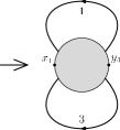
Iterating this operation maximally we can always reduce a spanning tree in the direct graph, with $n-1$ lines, obtaining a rosette. We recall that a rosette is simply a ribbon graph with a single vertex. The rosettes we consider all have a root (i.e. an external line on $\bar{v}$), and a cyclic ordering to turn around, e.g. counterclockwise. We always draw the rooted rosette so that no line arches above the root. This defines uniquely a numbering of the halflines (see Figure D.3, where the arrows represent the former line orientations).

Figure D.3: A Rooted Rosette

The second topological operation is the reduction of a tree line in the dual graph, exactly like the previous operation. Therefore it deletes this line in the direct graph. The resulting direct graph again keeps the same genus (remember that the genus of a graph is the same as the one of its dual). Iterating these two operations maximally we can always reduce completely a direct tree with $n-1$ lines and a dual tree with $f-1$ lines. We end up with a graph which we call a superrosette, which has only one vertex and one face (therefore its dual has one vertex and one face and is also a superrosette) (see Figure D.4).

Figure D.4: A SuperRosette

The third operation is a genus reduction on a rosette. We define a nice crossing in a rosette to be a pair of lines such that the end point of the first is the successor in the rosette of the starting point of the other (in the natural cyclic order of the rosette). This ensures that the two lines have a common “internal face". When there are crossings in the rosette, it is easy to check that there exists at least one such nice crossing, for instance lines 2-5 and 4-8 in Figure D.3.

The genus reduction consists in deleting the lines of a nice crossing and interchanging all the halflines encompassed by the first line with those encompassed by the second line, see Figure D.5. This operation which we call the “third Filk Move" decreases the number of lines by two, glues again the faces in a coherent way, and decreases the genus by one.

Figure D.5: The Third Filk Move

We need then to compute the determinant of $B^{\prime}$ matrices corresponding to reduced graphs of the type:

$$\begin{pmatrix}\sum_{i\neq j}\omega(i,j)\eta_{li}(-1)^{i+j+1}\eta_{l^{\prime}j}&\sum_{i\in v}(-1)^{i+1}\eta_{li}\\ \sum_{i\in v}(-1)^{i}\eta_{li}&0\\ \end{pmatrix}\ .$$ (4.42)

As the graph is orientable and up to a possible overall sign we can cast the matrix into the form:

$$\begin{pmatrix}\sum_{i\neq j}\omega(i,j)\varepsilon_{li}\varepsilon_{l^{\prime}j}&\sum_{i\in v}\varepsilon_{li}\\ -\sum_{i\in v}\varepsilon_{li}&0\\ \end{pmatrix}\ .$$ (4.43)

We claim:

Lemma D.3.4

The above determinant is:

• $0$ if the graph has more than one face,

• $2^{2g}$ if the graph has exactly one face.

Proof We reduce a tree. At each step we have a big vertex (the “rosette in the making") $V$ and a small vertex $v$ bound to $V$ by a line $l=(i,j)$ which we contract. We then have at each step a Pfaffian $\int\prod_{d\chi_{l}d\psi_{v}}e^{-B^{\prime}}$ where

$$B^{\prime} = \sum_{l,l^{\prime}}\chi_{l}\big{(}\sum_{i\neq j;i,j\in V}\omega(i,j)\varepsilon_{li}\varepsilon_{l^{\prime}j}+\sum_{i\neq j;i,j\in v}\omega(i,j)\varepsilon_{li}\varepsilon_{l^{\prime}j}\big{)}\chi_{l^{\prime}}$$ (4.44)

$$+ \sum_{l,v}\chi_{l}\varepsilon_{lv}\psi_{v}\ .$$

At each step we use a permutation to put $l$ at the first place in the matrix. Note that this permutation has nothing to do with the ordering of the halflines. The terms containing $\chi_{l}$ or $\psi_{v}$ at each step are:

$$B^{\prime}_{l}= \chi_{l}\varepsilon_{li}\sum_{l^{\prime}}\big{(}\sum_{i\neq p;p\in V}\omega(i,p)\varepsilon_{l^{\prime}p}+\sum_{j\neq k;k\in v}\omega(j,k)\varepsilon_{l^{\prime}k}\big{)}\chi_{l^{\prime}}$$ (4.45)

$$+\chi_{l}\varepsilon_{lj}\psi_{v}-\sum_{l^{\prime\prime}}\sum_{k\in v;k\neq j}\chi_{l^{\prime\prime}}\varepsilon_{l^{\prime\prime}k}\psi_{v}\ .$$

We perform the triangular change of variables:

$$\bar{\chi_{l}} = \chi_{l}-\varepsilon_{lj}\sum_{l^{\prime\prime}}\sum_{k\in v;k\neq j}\varepsilon_{l^{\prime\prime}k}\chi_{l^{\prime\prime}}$$ (4.46)

$$\bar{\psi_{v}} = \varepsilon_{lj}\psi_{v}+\varepsilon_{li}\sum_{l^{\prime}}\big{(}\sum_{i\neq p;p\in V}\omega(i,p)\varepsilon_{l^{\prime}p}+\sum_{i<k;k\in v}\omega(i,k)\varepsilon_{l^{\prime}k}\big{)}\chi_{l^{\prime}}$$

Under this change of variable:

$$B^{\prime}_{l} = \chi_{l}\bar{\psi_{v}}-\sum_{l^{\prime\prime}}\sum_{k\in v;k\neq j}\chi_{l^{\prime\prime}}\varepsilon_{l^{\prime\prime}k}\psi_{v}$$ (4.47)

$$= \bar{\chi_{l}}\bar{\psi_{v}}-\varepsilon_{li}\varepsilon_{lj}\sum_{l^{\prime\prime}}\sum_{l^{\prime}}\chi_{l^{\prime\prime}}\big{(}\sum_{k\in v;k\neq j}\sum_{p\in V;i\neq p}\omega(i,p)\varepsilon_{l^{\prime\prime}k}\varepsilon_{l^{\prime}p}$$

$$+ \sum_{k\in v;k\neq j}\sum_{r\in v;j\neq r}\omega(j,r)\varepsilon_{l^{\prime\prime}k}\varepsilon_{l^{\prime}r}\big{)}\chi_{l^{\prime}}$$

As $l$ is orientable $\varepsilon_{li}\varepsilon_{lj}=-1$, so that the new term corresponds exactly to a new big vertex $\tilde{V}$ where the ordered halflines $k$ of the small vertex $v$ replace the halfline $i\in l$. We continue this procedure until we have reduced a complete tree in our graph. The remaining Pfaffian is of the form:

$$B^{\prime}=\sum_{l<l^{\prime};l\cap l^{\prime}}\chi_{l}\big{(}\sum_{i\neq j;i,j\in V}\omega(i,j)\varepsilon_{li}\varepsilon_{l^{\prime}j}\big{)}\chi_{l^{\prime}}$$ (4.48)

where $l<l^{\prime}$ means that the starting halfline of $l$ precedes the end halfline of $l^{\prime}$ in the final rosette vertex $R$.

When two lines in the rosette do not cross, in both sums over $i$ and $j$ above the two endpoints of any of the two lines add and give zero. Consider now two lines $l_{1}=(i_{1},j_{1})$ and $l_{2}=(i_{2},j_{2})$ which cross each other, i.e. such that $i_{1}<i_{2}<j_{1}<j_{2}$. We have:

$$\chi_{l_{1}}(\varepsilon_{l_{1}i_{1}}\varepsilon_{l_{2}i_{2}}+\varepsilon_{l_{1}i_{1}}\varepsilon_{l_{2}j_{2}}+\varepsilon_{l_{1}j_{1}}\varepsilon_{l_{2}j_{2}}-\varepsilon_{l_{1}j_{1}}\varepsilon_{l_{2}i_{2}})\chi_{l_{2}}=2\chi_{l_{1}}\varepsilon_{l_{1}i_{1}}\varepsilon_{l_{2}i_{2}}\chi_{l_{2}}.$$ (4.49)

Changing the variables $\chi_{l}\rightarrow\varepsilon_{li}\chi_{l}$ and writing $l\cap l^{\prime}$ if $l$ crosses $l^{\prime}$ we have:

$$\frac{B^{\prime}}{2}=\sum_{l<l^{\prime};l\cap l^{\prime}}\chi_{l}\chi_{l^{\prime}}\ .$$ (4.50)

We perform a new simplification trick which we call the “third Filk move". We can pick two lines $l_{1}$ and $l_{2}$ which form a “nice crossing", i.e. the start of $l_{2}$ immediately precedes the end of $l_{1}$ in the rosette. We define the variables:

$$\bar{\chi}_{l_{1}}=\chi_{l_{1}}+\sum_{l^{\prime}<l_{2};l^{\prime}\cap l_{2}}\chi_{l^{\prime}}-\sum_{l^{\prime\prime}>l_{2};l^{\prime\prime}\cap l_{2}}\chi_{l^{\prime\prime}},$$

$$\bar{\chi}_{l_{2}}=\chi_{l_{2}}-\sum_{l^{\prime}<l_{1};l^{\prime}\cap l_{1}}\chi_{l^{\prime}}+\sum_{l^{\prime\prime}>l_{1};l^{\prime\prime}\cap l_{1}}\chi_{l^{\prime\prime}}\;,$$ (4.51)

and get:

$$\bar{\chi}_{l_{1}}\bar{\chi}_{l_{2}} = \chi_{l_{1}}\chi_{l_{2}}-\chi_{l_{1}}\sum_{l^{\prime}<l_{1};l^{\prime}\cap l_{1}}\chi_{l^{\prime}}+\chi_{l_{1}}\sum_{l^{\prime\prime}>l_{1};l^{\prime\prime}\cap l_{1}}\chi_{l^{\prime\prime}}$$

$$+\sum_{l^{\prime}<l_{2};l^{\prime}\cap l_{2}}\chi_{l^{\prime}}\chi_{l_{2}}-\sum_{l^{\prime\prime}>l_{2};l^{\prime\prime}\cap l_{2}}\chi_{l^{\prime\prime}}\chi_{l_{2}}$$

$$+(\sum_{l^{\prime}<l_{2};l^{\prime}\cap l_{2}}\chi_{l^{\prime}}-\sum_{l^{\prime\prime}>l_{2};l^{\prime\prime}\cap l_{2}}\chi_{l^{\prime\prime}})(-\sum_{l^{\prime}<l_{1};l^{\prime}\cap l_{1}}\chi_{l^{\prime}}+\sum_{l^{\prime\prime}>l_{1};l^{\prime\prime}\cap l_{1}}\chi_{l^{\prime\prime}})\ .$$

Denoting $B^{\prime}_{l_{1}l_{2}}$ all the terms which contain either $l_{1}$ or $l_{2}$ in $B^{\prime}$ and consistently denoting $l_{p}$ the lines which cross $l_{1}$ and $l_{q}$ those which cross $l_{2}$ we have:

$$B^{\prime}_{l_{1}l_{2}} = \bar{\chi_{l_{1}}}\bar{\chi_{l_{2}}}+\sum_{l_{q}<l_{2};l_{q}\cap l_{2}}\chi_{l_{q}}\sum_{l_{p}<l_{1};l_{p}\cap l_{1}}\chi_{l_{p}}-\sum_{l_{q}>l_{2};l_{q}\cap l_{2}}\chi_{l_{q}}\sum_{l_{p}<l_{1};l_{p}\cap l_{1}}\chi_{l_{p}}$$ (4.53)

$$- \sum_{l_{q}<l_{2};l_{q}\cap l_{2}}\chi_{l_{q}}\sum_{l_{p}>l_{1};l_{p}\cap l_{1}}\chi_{l_{p}}+\sum_{l_{q}>l_{2};l_{q}\cap l_{2}}\chi_{l_{q}}\sum_{l_{p}>l_{1};l_{p}\cap l_{1}}\chi_{l_{p}}\ .$$

Suppose that $l_{q}$ is the first line crossing $l_{2}$ and $l_{p}$ is the last line crossing $l_{1}$. Suppose moreover that $l_{q}<l_{2}$, $l_{p}<l_{1}$. When changing to the new variables we must add to the rosette factor a term of the first type in the above expression $\chi_{l_{q}}\chi_{l_{p}}$. What is the effect of such a term? If $l_{p}<l_{q}$ we have a crossing $\chi_{l_{p}}\chi_{l_{q}}$ and adding the above term gives zero. If $l_{p}>l_{q}$ adding the extra term acts like a new crossing. In both cases this amounts to permute the endpoints of $l_{p}$ and $l_{q}$. We can check that this holds in fact in all cases, and that by induction the extra terms in equation (4.53) permute all the legs of $l_{p}$ type with all the legs of $l_{q}$ type. We conclude that:

$$B^{\prime}=\bar{\chi_{l_{1}}}\bar{\chi_{l_{2}}}+B^{\prime}_{l_{p}\leftrightarrow l_{q}}\ ,$$ (4.54)

which is the content of our “third Filk move".

With this change of variables in the Pfaffian we see that contracting the lines of the tree through first Filk moves, and reducing the genus on the rosette through third Filk moves, we end up with a final Pfaffian which is $\pm 2^{g}$, taking into account the factors $2$ in (4.50), hence a determinant which is $2^{2g}$.

Suppose that the initial graph has $L$ propagators, $n$ vertices and $F$ faces. We have $2-2g=n-L+F$. We can reduce $n-1$ lines of a tree and $g$ nice crossings. The remaining rosette will have $L_{\mathrm{rest}}=F-1$ propagators, with no crossing. The only way for the remaining Pfaffian not to be zero is to have $F=1$. This completes the proof of Lemma D.3.4. $\Box$

Returning to the initial problem, we know that in order for the final graph to have a single face we need to reduce a tree $\tilde{T}$ in the dual graph ${\cal G}$. So when $I$ is maximal, $J$ must contain a tree in ${\cal G}$. But $J$ cannot be too big either, because the complement of $J$ must contain a tree in $G$ otherwise we cannot pair all hypermomenta variables. We say that $J$ is admissible if

• it contains a tree $\tilde{T}$ in the dual graph

• its complement contains a tree $T$ in the direct graph

• The rosette obtained by removing the lines of $J$ and contracting the lines of $T$ is a superrosette, hence has a single face.

In particular if $J$ is admissible, we have $F-1\leq|J|\leq F-1+2g$, and $k_{j}=|J|-F+1$ is even and obeys $0\leq k_{J}\leq 2g$.

We have altogether proved that:

Lemma D.3.5

Suppose $I$ is maximal, i.e. contains all lines. The integer $n_{I,J}$ in (4.41) is non zero if and only if $J$ is admissible, in which case $n_{I,J}^{2}=2^{2g-k_{J}}$

For $I$ maximal and $J$ admissible we have $k_{I,J}=k_{J}$. Hence using positivity to keep the terms with maximal $I$ that we have identified, we get

$$HU_{G,{\bar{v}}}\geq\sum_{J\ {\rm admissible}}(2s)^{2g-k_{J}}\prod_{l\in J}t_{l}\ .$$ (4.55)

>From this formula power counting follows easily by finding the leading terms under scaling of all $t^{\prime}s$ to 0, which are the ones with minimal $J$. They correspond to $J$’s which are trees in ${\cal G}$, hence which have $k_{J}=0$. Keeping only these terms in (4.55) we have the weaker bound:

$$HU_{G,{\bar{v}}}\geq(2s)^{2g}\sum_{J\ {\rm tree}\ \in\cal{G}}\prod_{l\in J}t_{l}\,.$$ (4.56)

At $D=4$, and for a graph of genus $g$ with $N$ external lines, using $2-2g=n+F-L$ and $L=2n-N/2$, we get from (4.56) at least a power counting in $\lambda^{2g+(N-4)/2}d\lambda$, so that we recover the correct power counting as function of the genus.

The commutative limit can be recovered easily as the limit $s\to 0$, in which case only the terms with $k_{J}=2g$ survive. These $J$’s are exactly the complements of the trees in $G$ so that $HU_{G,{\bar{v}}}$ reduce to the usual commutative Symanzik polynomial $U_{G}$ in the limit $s\to 0$.

It is interesting to notice that since $s=1/4\theta\Omega$ this limit $s\to 0$ seems to correspond to $\theta\to\infty$. But this is an artefact of our conventions and use of the direct space representation. Indeed in the limit $\theta\to\infty$ the vertex in $x$-space becomes the usual vertex in $p$-space of the commutative theory, whereas in the limit $\theta\to 0$ the vertex in $x$-space becomes the usual vertex in $x$-space of the commutative theory! This explains this paradox (remark that the usual parametric representation (4.5) has $p$-space external variables).

Remark also that for planar graphs the complement of a tree in the dual graph is a tree in the ordinary graph, hence (4.55) and (4.56) are identical in this case, as the sum over compatible $J$’s reduce to a sum over trees of either $G$ or ${\cal G}$.

The canonical polynomial $HU_{G}$ can be analyzed in a similar way, but there we need to take out one factor $c$, to pair to the additional hypermomentum in the Pfaffian, so that $|I|$ is at most $L-1$; and the leading terms have one additional $t$ factor when compared to $HU_{G,{\bar{v}}}$ (see Section D.5 for examples).

The power counting improvement in the number of faces broken by external fields is obtained after smearing external positions with smooth test functions. For this improvement we analyze now the second hyperbolic polynomial.

D.4 The Second Hyperbolic Polynomial

We analyse only the $HV_{G,{\bar{v}}}$ polynomial, as the canonical $HV_{G}$ can be obtained easily afterwards. The $P$ matrix in (4.18)-(4.19) has elements:

$$P_{eu_{l}} =-\sum_{i\neq e}\omega(i,e)\varepsilon_{li}\frac{\sigma}{4\theta\Omega}\,,\ P_{ev_{l}} =-\sum_{i\neq e}\omega(i,e)\eta_{li}\frac{\sigma}{4\theta\Omega}\,,$$ (4.57)

$$P_{ep_{v}} =-\sum_{v;e\in v}(-1)^{e+1}\frac{\sigma}{\Omega}\,,\ P_{\bar{p}u_{l}} =\frac{\sigma}{\Omega}\,.$$ (4.58)

Note that all the elements of $P$ are multiples of $\sigma$. Upon transposition of $P$ and multiplication we will recover a minus sign. Therefore the quadratic form in the external positions (and hypermomentum $\bar{p}$) in (4.19) is:

$$\begin{pmatrix}x_{e}&\bar{p}\\ \end{pmatrix}PQ^{-1}P^{t}\begin{pmatrix}x_{e}\\ \bar{p}\end{pmatrix} = -x_{e_{1}}P_{e_{1}\tau}Q^{-1}_{\tau\tau^{\prime}}P_{e_{2}\tau^{\prime}}x_{e_{2}}-x_{e_{1}}P_{e_{1}\tau}Q^{-1}_{\tau\tau^{\prime}}P_{\bar{p}\tau^{\prime}}\bar{p}$$ (4.59)

$$-\bar{p}P_{\bar{p}\tau}Q^{-1}_{\tau\tau^{\prime}}P_{e_{2}\tau^{\prime}}x_{e_{2}}-\bar{p}P_{\bar{p}\tau}Q^{-1}_{\tau\tau^{\prime}}P_{\bar{p}\tau^{\prime}}\bar{p}\,.$$

The inverse matrix of $Q$ being of the form

$$Q^{-1}_{\tau\tau^{\prime}}=\frac{(A+B)^{-1}_{\tau\tau^{\prime}}+(A-B)^{-1}_{\tau\tau^{\prime}}}{2}\otimes I_{D}+\frac{(A+B)^{-1}-(A-B)^{-1}}{2}\otimes\sigma\,,$$ (4.60)

we conclude that the quadratic form has a real part given by the $I_{D}$ terms and an imaginary (oscillating) part given by the $\sigma$ terms: the power counting we are looking for can be deduced solely from the former. To ease the writing we generically denote the set $x_{e},\bar{p}$ by $x_{e}$. Also, let $\mathrm{Pf}(B_{\hat{K}\hat{\tau}})$ be the Pfaffian of the matrix obtained from $B$ by deleting the lines and columns in the set ${K,\tau}$, where again $K=I\cup J$ can be decomposed according to short and long variables. We have the analog of (4.37):

$$\frac{HV_{G,{\bar{v}}}}{HU_{G,{\bar{v}}}}(X_{e})=\frac{1}{{\rm det}(A+B)}\sum_{K}\prod_{i\in K}a_{ii}\Big{[}\sum_{e_{1}}x_{e_{1}}\sum_{\tau\notin K}P_{e_{1}\tau}\varepsilon_{K\tau}\mathrm{Pf}(B_{\hat{K}\hat{\tau}})\Big{]}^{2}\,.$$ (4.61)

Multiplying by the product of $t$’s to compensate for the same product in $HU_{G,{\bar{v}}}$ we get:

Lemma D.4.1

The real part $HV^{R}_{G,v}$ of the quadratic form in the external positions is:

$$\frac{HV^{R}_{G,{\bar{v}}}}{HU_{G,{\bar{v}}}}(x_{e})=\frac{1}{HU_{G,{\bar{v}}}}\sum_{K}\prod_{i\not\in K}t_{i}\Big{[}\sum_{e_{1}}x_{e_{1}}\sum_{\tau\notin K}P_{e_{1}\tau}\varepsilon_{K\tau}\mathrm{Pf}(B_{\hat{K}\hat{\tau}})\Big{]}^{2}\,.$$ (4.62)

Proof : We represent the matrix elements $Q^{-1}_{\tau\tau^{\prime};\otimes K_{d}}$ by Grassmann integrals. As $(A+B)=(A-B)^{t}$ we have, for the first part of (4.60):

$$Q^{-1}_{\tau\tau^{\prime};\otimes I_{D}} = \frac{1}{2}[(A+B)^{-1}_{\tau\tau^{\prime}}+(A-B)^{-1}_{\tau\tau^{\prime}})$$ (4.63)

$$= \frac{1}{2{\rm det}(A+B)}\int(d\bar{\psi}d\psi)[\psi_{\tau}\bar{\psi}_{\tau^{\prime}}+\psi_{\tau^{\prime}}\bar{\psi}_{\tau}]e^{-\bar{\psi}(A+B)\psi}\,.$$

We perform the Pfaffian change of variables (of Jacobian $\imath$):

$$\psi_{j}=\frac{\chi_{j}+\imath\eta_{j}}{\sqrt{2}};\leavevmode\nobreak\ \bar{\psi}=\frac{\chi_{j}-\imath\eta_{j}}{\sqrt{2}}\,,$$ (4.64)

and we get (recalling that $d=2L+n-1$):

$$Q^{-1}_{\tau\tau^{\prime};\otimes I_{D}} = \frac{1}{2{\rm det}(A+B)}\int\prod_{j}(d\eta_{j}d\chi_{j})\imath^{d}[\imath(\eta_{\tau}\chi_{\tau^{\prime}}+\eta_{\tau^{\prime}}\chi_{\tau})]$$ (4.65)

$$e^{-\frac{1}{2}(\chi A\chi-\imath\eta A\chi+\chi B\chi-\imath\eta B\chi+\imath\chi A\eta+\eta A\eta+\imath\chi B\eta+\eta B\eta)}\,.$$

As $B$ is antisymmetric the crossed terms in $B$ add to zero; as $A$ is diagonal the crossed terms are the only ones which survive. Reordering the measure and developping the exponential term in $A$ we get:

$$\frac{1}{2{\rm det}(A+B)}\int\prod_{j}(d\eta_{j}d\chi_{j})\imath^{d}[-\imath(\chi_{\tau^{\prime}}\eta_{\tau}+\chi_{\tau}\eta_{\tau^{\prime}})]e^{-\frac{1}{2}(\chi B\chi+\eta B\eta)+\imath\eta A\chi}$$

$$=\frac{1}{2{\rm det}(A+B)}\int\prod d\eta\prod d\chi(-1)^{\frac{d^{2}}{2}}(-\imath)(\chi_{\tau^{\prime}}\eta_{\tau}+\chi_{\tau}\eta_{\tau^{\prime}})$$

$$\sum_{K}\prod_{i\in K}\imath^{|K|}a_{ii}\eta_{i}\chi_{i}e^{-\frac{1}{2}(\chi B\chi+\eta B\eta)}\,.$$ (4.66)

Factorizing the sums over elements in $A$ and reordering the variables we finally get:

$$Q^{-1}_{\tau\tau;\otimes I_{D}}=\frac{1}{2{\rm det}(A+B)}\sum_{K}\prod_{i\in K}a_{ii}(-1)^{\frac{d^{2}}{2}}(-\imath)\imath^{|K|}(-1)^{\frac{|K|(|K|+1)}{2}}$$

$$\int d\eta\int d\chi\prod_{i\in K}\chi_{i}\prod_{i\in K}\eta_{i}(\chi_{\tau^{\prime}}\eta_{\tau}+\chi_{\tau}\eta_{\tau^{\prime}})e^{-\frac{1}{2}(\chi B\chi+\eta B\eta)}\,.$$ (4.67)

Note that the last integrals are nonzero only if $d-|K|-1$ is even, which implies that the global sign in the above expression is always plus. The remaining Grassmann integrals can be expressed as:

$$\int\prod_{\alpha=1\dotsc d}d\chi_{\alpha}\prod_{i\in K}\chi_{i}\chi_{\tau}e^{-\frac{1}{2}\chi B\chi}=\varepsilon_{K\tau}\mathrm{Pf}(B_{\hat{K}\hat{\tau}})\,,$$ (4.68)

where $\varepsilon_{K\tau}$ is the signature of the permutation

$$1\dotsc d\rightarrow 1\dotsc\hat{i_{1}}\dotsc\hat{i_{p}}\dotsc\hat{i_{\tau}}\dotsc di_{\tau}i_{p}\dotsc i_{1}\,.$$ (4.69)

We have then:

$$Q^{-1}_{\tau\tau^{\prime};\otimes I_{D}}=\frac{1}{{\rm det}(A+B)}\sum_{K}\prod_{i\in K}a_{ii}\varepsilon_{K\tau}\mathrm{Pf}(B_{\hat{K}\hat{\tau}})\varepsilon_{K\tau^{\prime}}\mathrm{Pf}(B_{\hat{K}\hat{\tau^{\prime}}})\,,$$ (4.70)

and the real part of the quadratic form is:

$$\sum_{e_{1},e_{2},\tau,\tau^{\prime}}-x_{e_{1}}P_{e_{1}\tau}\frac{1}{|A+B|}\sum_{K}\prod_{i\in K}a_{ii}\varepsilon_{K\tau}\mathrm{Pf}(B_{\hat{K}\hat{\tau}})\varepsilon_{K\tau^{\prime}}\mathrm{Pf}(B_{\hat{K}\hat{\tau^{\prime}}})P_{e_{2}\tau^{\prime}}x_{e_{2}}$$

$$=-\frac{1}{{\rm det}(A+B)}\sum_{K}\prod_{i\in K}a_{ii}\Big{[}\sum_{e_{1}}x_{e_{1}}\sum_{\tau\notin K}P_{e_{1}\tau}\varepsilon_{K\tau}\mathrm{Pf}(B_{\hat{K}\hat{\tau}})\Big{]}^{2}\,.$$ (4.71)

This ends the proof of (4.62). $\Box$

Using similar methods one can prove that the imaginary part of the inverse matrix elements is:

$$Q^{-1}_{\tau\tau^{\prime};\otimes\sigma}=\frac{1}{{\rm det}(A+B)}\sum_{K}\prod_{i\in K}a_{ii}\varepsilon_{K\tau\tau^{\prime}}\mathrm{Pf}(B_{\hat{K}\hat{\tau}\hat{\tau^{\prime}}})\varepsilon_{K}\mathrm{Pf}(B_{\hat{K}})\,,$$ (4.72)

and consequently the contribution to the quadratic form is:

$$-\frac{1}{{\rm det}(A+B)}\sum_{K}\prod_{i\in K}a_{ii}\varepsilon_{K}\mathrm{Pf}(B_{\hat{K}})$$

$$\Big{[}\sum_{e_{1},e_{2}}\Big{(}\sum_{\tau\tau^{\prime}}P_{e_{1}\tau}\varepsilon_{K\tau\tau^{\prime}}\mathrm{Pf}(B_{\hat{K}\hat{\tau}\hat{\tau^{\prime}}})P_{e_{2}\tau^{\prime}}\Big{)}x_{e_{1}}\sigma x_{e_{2}}\Big{]}\,.$$ (4.73)

D.4.1 Leading terms

The last step of our analysis is to find the leading terms in eq. (4.62). In order to do this one must find under which conditions Pfaffians like:

$$\varepsilon_{K\tau}\mathrm{Pf}(B_{\hat{K}\hat{\tau}})=\int\prod_{\alpha=1\dotsc d}d\chi_{\alpha}\prod_{i\in K}\chi_{i}\chi_{\tau}e^{-\frac{1}{2}\chi B\chi}\,,$$ (4.74)

are nonzero.

A priori one can exploit the $\delta$ functions associated with each external vertex to simplify the oscillating factor involving the external position. These manipulations do not have any effect on the form of $HV$ but can be used to set some $P_{ev_{l}}$ and $P_{eu_{l}}$ to zero. This is always the case if our graph does not have any vertex with two opposite external points. We conclude that the power counting behavior of the second polynomial should entirely be given by $P_{ev_{e}}$ and consequently by terms like:

$$\varepsilon_{Kv_{e}}\mathrm{Pf}(B_{\hat{K}\hat{v_{e}}})=\int\prod_{\alpha=1\dotsc d}d\chi_{\alpha}\prod_{i\in K}\chi_{i}\psi_{v_{e}}e^{-\frac{1}{2}\chi B\chi}\,.$$ (4.75)

The reasoning is similar to that we used to find the leading contributions in the $HU_{G,v}$. We must find a nonzero Pfaffian multiplied by all the $c$’s and the smallest number of $t$’s possible, hence corresponding to $K=I\cup J$ with $I=[1,...L]$ maximal and $J$ minimal. One could find a change of variables similar to those of lemma D.3.4, but we will use here a slightly different approach.

We introduce a dummy Grassmann variable $\Psi$ in the Pfaffian integrals, to have:

$$\varepsilon_{Kv_{e}}\mathrm{Pf}(B_{\hat{K}\hat{v_{e}}})=\int\prod_{\alpha=1\dotsc d}d\chi_{\alpha}d\Psi\ \Psi\prod_{i\in K}\chi_{i}\psi_{v_{e}}e^{-\frac{1}{2}\chi B\chi}\,.$$ (4.76)

Next we exponentiate $\Psi\psi_{v_{e}}$ and pass to the Pfaffian of a modified matrix $B^{\prime}$ (corresponding to a modified graph $G^{\prime}$). The modified graph is obtained from $G$ by adding a line $l_{0}$ from $x_{e}$ to the root external line. Moreover, following the reasoning of lemma D.3.4 we see that our Pfaffian is not modified if we impose that the dummy line is constrained to be a tree line in the direct graph $G^{\prime}$, i.e. has to pair with an hypermomentum variable. We then have a one to one correspondence between the leading term in $HV_{G,{\bar{v}}}$ and the leading terms for the first polynomial of the modified graph $HU_{G^{\prime},{\bar{v}}}$ in which the dummy line $l_{0}$ is chosen as a tree line.

In order to conclude we need only to compute the genus of the modified graph $G^{\prime}$. Suppose the external point $x_{e}$ broke another face than the root external point. The dummy line we added will identify the two faces so that $G^{\prime}$ has $n^{\prime}=n$, $L^{\prime}=L+1$, $F^{\prime}=F-1$ and $n^{\prime}-L^{\prime}+F^{\prime}=2-2g^{\prime}$, so that $g^{\prime}=g+1$. If, on the other hand, $x_{e}$ broke the same face as the root halfline, the dummy line will part the latter in two different faces. We then have $F^{\prime}=F+1$ and consequently $g^{\prime}=g$.

We note that to any tree in $G^{\prime}$ constrained to contain the dummy line $l_{0}$ there corresponds a two-tree $T_{2}$ in $G$, that is a tree minus a line (by removing this dummy line).

Therefore by Lemma III.4 the Pfaffian we are considering is non zero only if the new reduced rosette, where the dummy line is contracted as a tree line, has exactly one face and $2g^{\prime}$ lines.

We obtain therefore the real part of $V_{G,{\bar{v}}}$ as a sum of positive terms and exact analogs of bounds (4.55) and (4.56). We say that $J$ is 2-admissible in $G$ if $J$ is admissible in $G^{\prime}$ and the dummy line $l_{0}$ is in a tree of $G^{\prime}$ contained in the complement of $J$.

Let $\tilde{G}$, be the graph obtained from $G$ by deleting the lines in $J$ and contracting the two-tree $T_{2}$. It has two faces, the one broken by the root and another one, $F_{J}$. This $F_{J}$ contains typically the external points belonging to several broken faces in the initial graph. The dummy line $l_{0}$ will link this two faces, but the topological structure of $G^{\prime}$ is the same no matter which external points are chosen in $F_{J}$. We will therefore obtain a sum over all this possible choices. We conclude that the bound analog to (4.55) is

$$HV^{R}_{G,{\bar{v}}}(x_{e})\geq\sum_{J\ {\rm 2-admissible\ in}\ G}(2s)^{2g^{\prime}-k_{J}}\prod_{l\in J}t_{l}[\sum_{e\in F_{J}}(-1)^{e}x_{e}]^{2}\;.$$ (4.77)

The analog of (4.56) is

$$HV^{R}_{G,{\bar{v}}}(x_{e})\geq\sum_{J\ {\rm tree\ in}\ {\cal G}^{\prime}}(2s)^{2g^{\prime}}\prod_{l\in J}t_{l}\ [\sum_{e\in F_{J}}(-1)^{e}x_{e}]^{2}\;.$$ (4.78)

This bound is the one useful to extract the power counting in the broken faces. Indeed when integrating the remaining external variables against fixed test functions and scaling each $t$ variable by $\lambda\to 0$, we recover the full exact power counting of $G$ namely in dimension $D=4$ the scaling $\lambda^{2g+(B-1)+(N-4)/2}d\lambda$. Indeed each broken face leads to a term in $e^{-[x_{e}+\dotsc]^{2}}$ for some external variable $x_{e}$ of the broken face, hence to an improved factor $\lambda$ when integrated against a fixed test function.

It is also possible to recover the second Symanzik polynomial as $s\to 0$ in (4.77); indeed for $k_{J}=2g^{\prime}$, we find that $J$ is the complement of a tree in $G^{\prime}$ containing $l_{0}$, hence of a two-tree in $G$. Moreover, in this case the face $F_{J}$ will be the external face of the conected component $E(T_{2})\in T_{2}$ not containing the root, and we recover the known invariant $(\sum_{e\in E(T_{2})}(-1)^{e+1}x_{e})^{2}$.

It remains to discuss the case with special “diagonal" vertices, that is with opposite external arguments as in Figure D.9. In this case bounds (4.77) and (4.78) still hold because although there is a sum of two Paffians in Lemma D.4.1, they cannot add up to 0; they correspond to graphs $G^{\prime}_{1}$ (of the same kind as before) and $G^{\prime}_{2}$ (of a new type, with one line erased) with genuses $g^{\prime}_{1}$ and $g^{\prime}_{2}=g^{\prime}_{1}-1$. These Pfafians have the same scaling in $s$ because there is an additional $s$ for $G^{\prime}_{2}$ coming from formula (4.57), but they have not the same power of 2 hence their sum cannot be zero again!

There is another modification: the alternate sum over a face no longer appear in (4.77) and in (4.78) if the root vertex itself is of this diagonal type which is the case for the “Broken Bubble" graph of Figure D.9. These modifications do not affect the power counting and their verification is left to the reader.

D.5 Examples

In this section we give the exact expressions for several of our polynomials. We recall that $s=(4\theta\Omega)^{-1}$.

Figure D.6: The Bubble graph

We start by the bubble graph, Figure D.6:

$$HU_{G,v} = (1+4s^{2})(t_{1}+t_{2}+t_{1}^{2}t_{2}+t_{1}t_{2}^{2})\,,$$

$$HV_{G,v} = t_{2}^{2}\Big{[}p_{2}+2s(x_{4}-x_{1})\Big{]}^{2}+t_{1}t_{2}\Big{[}2p_{2}^{2}+(1+16s^{4})(x_{1}-x_{4})^{2}\Big{]}\,,$$

$$+t_{1}^{2}\Big{[}p_{2}+2s(x_{1}-x_{4})\Big{]}^{2}$$

$$HU_{G} = 4(t_{1}+t_{2})^{2}\,,$$

$$HV_{G} = (1+4s^{2})\Big{[}(x_{1}-x_{4}+y_{1}-y_{4})^{2}(t_{1}+t_{2})$$ (4.79)

$$+(x_{1}-x_{4}-y_{1}+y_{4})^{2}(t_{1}t_{2}^{2}+t_{2}t_{1}^{2})\Big{]}\,.$$

The first two terms in $HU_{G,v}$ are the leading ones we previously exhibited. For the $HV_{G,v}$ we see that the scaling of the quadratic form will be in $O(1)$, which was expected as we do have only one broken face. Furthermore $HU_{G}$ scales in $t^{2}$, as expected, and the first term in the quadratic form $HU_{G}/HV_{G}$ is exactly the required one to reconstitute the $\delta$ function on the external legs in the $UV$ region. The term $t_{1}t_{2}(x_{1}-x_{4})^{2}$ in $HV_{G,\bar{v}}$ is one of the leading terms previousely computed. It comes from the graphs $G^{\prime}$ in which either $x_{1}$ or $x_{4}$ are linked to the root by the dummy line, and both lines $1$ and $2$ are chosen in the set $J$ in $\cal{G^{\prime}}$.

Then comes the sunshine graph Fig. D.7:

Figure D.7: The Sunshine graph

$$HU_{G,v} = \Big{[}t_{1}t_{2}+t_{1}t_{3}+t_{2}t_{3}+t_{1}^{2}t_{2}t_{3}+t_{1}t_{2}^{2}t_{3}+t_{1}t_{2}t_{3}^{2}\Big{]}(1+8s^{2}+16s^{4})$$

$$+16s^{2}(t_{2}^{2}+t_{1}^{2}t_{3}^{2})\,,$$

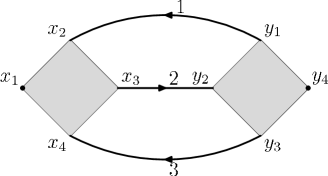
$$HU_{G} = t_{1}t_{2}t_{3}(1+64s^{4})$$ (4.80)

$$+\Big{[}t_{1}^{2}t_{2}+t_{1}t_{2}^{2}+t_{1}^{2}t_{3}+t_{2}^{2}t_{3}+t_{1}t_{3}^{2}+t_{2}t_{3}^{2}\Big{]}(4+16s^{2})\,.$$

Here we identify also the leading contributions in $HU_{G,v}$, and the extra scaling factor in the $HU_{G}$.

For the nonplanar sunshine graph (see Fig. D.8) we have:

Figure D.8: The Non-planar Sunshine graph

$$HU_{G,v} = \Big{[}t_{1}t_{2}+t_{1}t_{3}+t_{2}t_{3}+t_{1}^{2}t_{2}t_{3}+t_{1}t_{2}^{2}t_{3}+t_{1}t_{2}t_{3}^{2}\Big{]}(1+8s^{2}+16s^{4})$$

$$+4s^{2}\Big{[}1+t_{1}^{2}+t_{2}^{2}+t_{1}^{2}t_{2}^{2}+t_{3}^{2}+t_{1}^{2}t_{3}^{2}+t_{2}^{2}t_{3}^{2}+t_{1}^{2}t_{2}^{2}t_{3}^{2}\Big{]}\,,$$

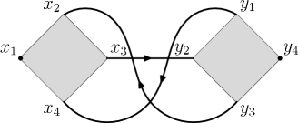
$$HU_{G} = 4\Big{[}t_{1}^{2}(t_{2}+t_{3})+t_{2}t_{3}(t_{2}+t_{3})+t_{1}(t_{2}^{2}+3t_{2}t_{3}+t_{3}^{2})\Big{]}$$ (4.81)

$$+16s^{2}\Big{[}t_{1}+t_{2}+t_{3}+t_{1}t_{2}^{2}t_{3}^{2}+t_{1}^{2}t_{2}t_{3}(t_{2}+t_{3})\Big{]}+64t_{1}t_{2}t_{3}s^{4}\,.$$

We note the improvement in the genus, as both $HU_{G,v}$ and $HU_{G,v}$ scale in $t^{-2}$ with respect to there planar counterparts.

For the broken bubble graph (see Fig. D.9) we have:

Figure D.9: The Broken Bubble Graph

$$HU_{G,v} = (1+4s^{2})(t_{1}+t_{2}+t_{1}^{2}t_{2}+t_{1}t_{2}^{2})\,,$$

$$HV_{G,v} = t_{2}^{2}\Big{[}4s^{2}(x_{1}+y_{2})^{2}+(p_{2}-2s(x_{3}+y_{4}))^{2}\Big{]}+t_{1}^{2}\Big{[}p_{2}+2s(x_{3}-y_{4})\Big{]}^{2}\,,$$

$$+t_{1}t_{2}\Big{[}8s^{2}y_{2}^{2}+2(p_{2}-2sy_{4})^{2}+(x_{1}+x_{3})^{2}+16s^{4}(x_{1}-x_{3})^{2}\Big{]}$$

$$+t_{1}^{2}t_{2}^{2}4s^{2}(x_{1}-y_{2})^{2}\,,$$

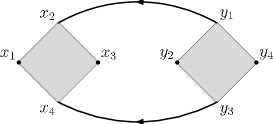
$$HU_{G} = 4(t_{1}+t_{2})^{2}\,,$$ (4.82)

$$HV_{G} = (t_{1}+t_{2})\Big{[}(y_{2}+y_{4}-x_{1}-x_{3})^{2}+4s^{2}(y_{2}-y_{4}-x_{1}-3x_{3})^{2}\Big{]}$$

$$+(t_{1}^{2}t_{2}+t_{1}t_{2}^{2})\Big{[}(y_{2}+y_{4}+x_{1}+x_{3})^{2}+4s^{2}(y_{2}-y_{4}+x_{1}+3x_{3})^{2}\Big{]}\,,$$

Note that $HU_{G,v}$ and $HU_{G}$ are identical with those of the bubble with only one broken face. It is natural, as the amelioration in the broken faces for a given graph can be seen only in the $HV_{G,v}$ and $HV_{G}$. Take $HV_{G}$. We see that we have two linear combinations which in the $UV$ region become an approximate $\delta$ function, whereas in the bubble graph with one broken face we had only one, therefore giving us the improvement in the broken faces. Similarely for the $HV_{G,v}$ we see that for the broken bubble we have three independent linear combinations which scale in $t^{-1}$ whereas for the bubble with only one broken face we only had two. The term $t_{1}t_{2}(x_{1}+x_{3})^{2}$ in $HV_{G,\bar{v}}$ is one of those computed in the previous section. Even if the two external points $x_{1}$ and $x_{3}$ do not belong to the same face they still appear summed, as we can chose the root halfline to be either $y_{2}$ and $y_{4}$ and we must add the contributions for each choice. This is an example of the slight modifications generated by the presence of "diagonal" vertices.

Figure D.10: The Half-Eye Graph

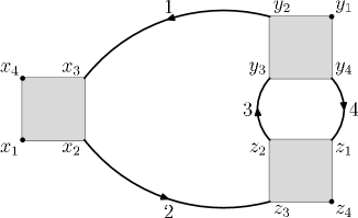
Finally, for the half-eye graph (see Fig. D.10), we start by defining:

$$A_{24}=t_{1}t_{3}+t_{1}t_{3}t_{2}^{2}+t_{1}t_{3}t_{4}^{2}+t_{1}t_{3}t_{2}^{2}t_{4}^{2}\,.$$ (4.83)

The $HU_{G,v}$ polynomial with fixed hypermomentum corresponding to the vertex with two external legs is:

$$(A_{24}+A_{14}+A_{23}+A_{13}+A_{12})(1+8s^{2}+16s^{4})$$

$$+t_{1}t_{2}t_{3}t_{4}(8+16s^{2}+256s^{4})+4t_{1}t_{2}t_{3}^{2}+4t_{1}t_{2}t_{4}^{2}$$

$$+16s^{2}(t_{3}^{2}+t_{2}^{2}t_{4}^{2}+t_{1}^{2}t_{4}^{2}+t_{1}^{2}t_{2}^{2}t_{3}^{2})+64s^{4}(t_{1}t_{2}t_{3}^{2}+t_{1}t_{2}t_{4}^{2})\,,$$

whereas with another fixed hypermomentum we get:

$$HU_{G,v_{2}} = (A_{24}+A_{14}+A_{23}+A_{13}+A_{12})(1+8s^{2}+16s^{4})$$ (4.84)

$$+t_{1}t_{2}t_{3}t_{4}(4+32s^{2}+64s^{4})+32s^{2}t_{1}t_{2}t_{3}^{2}+32s^{2}t_{1}t_{2}t_{4}^{2}$$

$$+16s^{2}(t_{3}^{2}+t_{1}^{2}t_{4}^{2}+t_{2}^{2}t_{4}^{2}+t_{1}^{2}t_{2}^{3}t_{3}^{2})\,.$$

Note that the leading terms are identical, the choice of the root perturbing only the non-leading ones. Moreover note the presence of the $t_{3}^{2}$ term. Its presence can be understood by the fact that in the sector $t_{1},t_{2},t_{4}>t_{3}$ the subgraph formed by the lines $1,2,4$ has two broken faces. This is the sign of a power counting improvement due to the additional broken face in that sector. To exploit it, we have just to integrate over the variables of line $3$ in that sector, using the second polynomial $HV_{G^{\prime},v}$ for the triangle subgraph $G^{\prime}$ made of lines $1,2,4$.

Finally the canonical $HU_{G}$ polynomial is:

$$HU_{G} = (4+16s^{2})(t_{1}^{2}t_{3}+t_{1}t_{3}^{2}+t_{2}^{2}t_{3}+t_{2}t_{3}^{2}+t_{1}^{2}t_{4}+t_{1}t_{4}^{2}+t_{2}^{2}t_{4}+t_{2}t_{4}^{2}$$ (4.85)

$$+t_{3}^{2}t_{4}+t_{3}t_{4}^{2}+t_{1}^{2}t_{2}t_{3}^{2}+t_{1}t_{2}^{2}t_{3}^{2}+t_{1}^{2}t_{2}t_{4}^{2}+t_{1}t_{2}^{2}t_{4}^{2}+t_{1}^{2}t_{2}^{2}t_{3}^{2}t_{4}$$

$$+t_{1}^{2}t_{2}^{2}t_{3}t_{4}^{2})+(8+32s^{2})(t_{1}t_{2}t_{3}+t_{1}t_{2}t_{4}+t_{1}t_{2}t_{3}^{2}t_{4}+t_{1}t_{2}t_{3}t_{4}^{2})$$

$$+(12+64s^{4})(t_{1}t_{3}t_{4}+t_{2}t_{3}t_{4}+t_{1}^{2}t_{2}t_{3}t_{4}+t_{1}t_{2}^{2}t_{3}t_{4})\,.$$

Acknowledgment

We are indebted to A. Abdesselam for his inspiring reference [67] and his help on the track to the Pfaffian analysis of Sections III-IV. We also thank M. Disertori, J. Magnen and F. Vignes-Tourneret for useful discussions during preparation of this work.

Annexe E Dimensional renormalization of NCQFT

R. Gurau, A. Tanasă

Using the recently introduced parametric representation of non-commutative quantum field theory, we implement here the dimensional regularization and renormalization of the vulcanized $\Phi^{\star 4}_{4}$ model on the Moyal space.

Keywords: non-commutative quantum field theory, dimensional regularization, dimensional renormalization

E.1 Introduction and motivation

Non-commutative geometry (see [22]) is one of the most appealing frameworks for the quantification of gravitation. Quantum field theory (QFT) on these type of spaces, called non-commutative quantum field theory (NCQFT) - for a general review see [25, 69]- is now one of the most appealing candidates for new physics beyond the Standard Model. Also, NCQFT arises as the effective limit of some string theoretical models [20, 51].

Moreover, NCQFT is well suited to the description of the physics in background fields and with non-local interactions, like for example the fractional quantum Hall effect [9, 10, 11].

However, naive NCQFT suffers from a new type of non renormalizable divergences, known as the ultraviolet (UV)/ infrared (IR) mixing. The simplest example of this kind of divergences is given by the nonplanar tadpole: it is UV convergent, but inserting it an arbitrary number of times in a loop gives rise to IR divergences.

Interest in NCQFT has been recently revived with the introduction of the Grosse-Wulkenhaar scalar $\Phi^{\star 4}_{4}$ model, in which the UV/IR mixing is cured: the model is renormalizable at all orders in perturbation theory [27, 29]. The idea of Grosse-Wulkenhaar was to modify the kinetic part of the action in order to satisfy the Langmann-Szabo duality [30] (which relates the infrared and ultraviolet regions). We refer to this modified theory as the vulcanized $\Phi^{\star 4}_{4}$ model.

A general proof, using position space and multiscale analysis, has then been given in [56], and the parametric representation of this model was computed in [39]. Furthermore, it was recently proved that that the vulcanized $\Phi^{\star 4}_{4}$ is better behaved than the commutative $\phi^{4}_{4}$ model: it does not have a Landau ghost [37, 38, 70].

In commutative QFT dimensional renormalization is the only scheme which respects the symmetries of gauge theories see [71, 72, 73]. It also is the appropriate setup for the Connes-Kreimer Hopf algebra approach to renormalization (see [65, 74] for the case of commutative QFT).

A second class of renormalizable NCQFT exists. These models, called covarinat, are characterized by a propagator which decays in position space as $x-y$ tends to infinity (like the Grosse-Wulkenhaar propagator of eq. (5.8)) but it oscillates when $x+y$ goes to infinity, rather than decaying. In this class of NCQFT models enters the non-commutative Gross-Neveu model and the Langmann-Szabo-Zarembo model [49]. The non-commutative orientable Gross-Neveu model was proven to be renormalizable at any order in perturbation theory [32]. The parametric representation was extended to this class of models [40]. For a general review of recent developments in the field of renormalizable NCQFT see [75].

The parametric representation introduced in [39] is the starting point for the dimensional regularization and renormalization performed in this paper. Our proof follows that of the commutative $\Phi^{\star 4}_{4}$ model, as presented in [71, 72].

This paper is organized as follows. Section E.2 is a summary of the parametric representation of the vulcanized $\Phi^{\star 4}_{4}$ model. The non-commutative equivalent $HU_{G}$ and $HV_{G}$ of the Symanzik polynomials $U_{G}$ and $V_{G}$ are recalled. In section E.3 we prove the existence in the polynomial $HU_{G}$ of some further leading terms in the ultraviolet (UV) regime. This is an improvement of the results of [39], needed to correctly identify the meromorphic structure of the Feynman amplitudes. In section E.4 we prove the factorization properties of the Feynman amplitudes. These properties are needed in order to prove that the pole extraction is equivalent to adding counterterms of the form of the initial lagrangean. This factorization is essential for the definition of a coproduct $\Delta$ necessary for the implementation of a Hopf algebra structure in NCQFT [76]. Section E.5 uses the results of the previous sections to perform the dimensional regularization, prove the counterterm structure for NCQFT and complete the dimensional renormalization program. Section E.6 is devoted to some conclusion and perspectives.

E.2 The non-commutative model

In this section we give a brief overview of the Grosse-Wulkenhaar $\Phi^{4}$ model. Our notations and conventions as well as some notions of diagrammatics and the results of the parametric representation follow [39].

To define the Moyal space of dimension $D$, we introduce the deformed Moyal product $\star$ on ${\mathbb{R}}^{D}$ so that

$$[x^{\mu},x^{\nu}]=i\Theta^{\mu\nu},$$ (5.1)

where the the matrix $\Theta$ is

$$\Theta=\begin{pmatrix}\begin{matrix}0&\theta\\ -\theta&0\end{matrix}&&0\\ &\ddots&\\ 0&&\begin{matrix}0&\theta\\ -\theta&0\end{matrix}\end{pmatrix}.$$ (5.2)

The associative Moyal product of two functions $f$ and $g$ on the Moyal space writes

$$(f\star g)(x) = \int\frac{d^{D}k}{(2\pi)^{D}}d^{D}y\,f(x+{\textstyle\frac{1}{2}}\Theta\cdot k)g(x+y)e^{\imath k\cdot y}$$ (5.3)

$$= \frac{1}{\pi^{D}|{\rm det}\Theta|}\int d^{D}yd^{D}z\,f(x+y)g(x+z)e^{-2\imath y\Theta^{-1}z}\;.$$

The Euclidian action introduced in [29] is

$$S=\int d^{4}x\left(\frac{1}{2}\partial_{\mu}\phi\star\partial^{\mu}\phi+\frac{\Omega^{2}}{2}(\tilde{x}_{\mu}\phi)\star(\tilde{x}^{\mu}\phi)+\frac{1}{2}m^{2}\,\phi\star\phi+\phi^{\star 4}\right)\,,$$ (5.4)

where

$$\tilde{x}_{\mu}=2(\Theta^{-1})_{\mu\nu}x^{\nu}\,.$$ (5.5)

The propagator of this model is the inverse of the operator

$$-\Delta+\Omega^{2}\tilde{x}^{2}.$$ (5.6)

The results we establish here hold for orientable models (in the sense of subsection E.2.1). This corresponds to a Grosse-Wulkenhaar model of a complex scalar field

$$S=\int d^{4}x\left(\frac{1}{2}\partial_{\mu}\bar{\phi}\star\partial^{\mu}\phi+\frac{\Omega^{2}}{2}(\tilde{x}_{\mu}\bar{\phi})\star(\tilde{x}^{\mu}\phi)+\bar{\phi}\star\phi\star\bar{\phi}\star\phi\right)\,.$$ (5.7)

Introducing $\tilde{\Omega}=2\Omega/\theta$, the kernel of the propagator is (Lemma $3.1$ of [36])

$$C(x,y)=\int_{0}^{\infty}\frac{\tilde{\Omega}d\alpha}{[2\pi\sinh(\alpha)]^{D/2}}e^{-\frac{\tilde{\Omega}}{4}\coth(\frac{\alpha}{2})(x-y)^{2}-\frac{\tilde{\Omega}}{4}\tanh(\frac{\alpha}{2})(x+y)^{2}}\;.$$ (5.8)

Using eq. (5.3) the interaction term in eq. (5.7) leads to the following vertex contribution in position space (see [56]

$$\delta(x_{1}-x_{2}+x_{3}-x_{4})e^{2i\sum_{1\leq i<j\leq 4}(-1)^{i+j+1}x_{i}\Theta^{-1}x_{j}}\,.$$ (5.9)

with $x_{1},\ldots,x_{4}$ the $4-$vectors of the positions of the $4$ fields incident to the vertex.

To any such vertex $V$ one associates a hypermomentum $p_{V}$ using the relation

$$\delta(x_{1}-x_{2}+x_{3}-x_{4})=\int\frac{dp_{V}}{(2\pi)^{4}}e^{p_{V}\sigma(x_{1}-x_{2}+x_{3}-x_{4})}\,.$$ (5.10)

E.2.1 Some diagrammatics for NCQFT; orientability

In this subsection we introduce some useful conventions and definitions, some of them used in [56] and [36] but also some new ones.

Let a graph $G$ with $n(G)$ vertices, $L(G)$ internal lines and $F(G)$ faces. The Euler characteristic of the graph is

$$2-2g(G)=n(G)-L(G)+F(G),$$ (5.11)

where $g(G)\in{\mathbb{N}}$ is the genus of the graph. Graphs divide in two categories, planar graph with $g(G)=0$, and non-planar graphs with $g(G)>0$. Let also $B(G)$ denote the number of faces broken by external lines and $N(G)$ be number of external points of the graph.

The “orientable” form eq .(5.9) of the vertex contribution of our model allows us to associate “+” sign to a corner $\bar{\phi}$ and a “-” sign to a corner $\phi$ of the vertex. These signs alternate when turning around a vertex. As the propagator allways relates a $\bar{\phi}$ to a $\phi$, the action in eq. (5.7) has orientable lines, that is any internal line joins a “-” corner to a “+” corner .

Consider a spanning tree ${\cal T}$ in $G$. In has $n-1$ lines and the remaining $L-(n-1)$ lines form the set $\cal L$ of loop lines. Amongst the vertices $V$ one chooses a special one $\bar{V}_{G}$, the root of the tree. One associates to any vertex $V$ the unique tree line which hooks to $V$ and goes towards the root.

We introduce now some topological operations on the graph which allow one to reexpress the oscillating factors coming from the vertices of the graph $G$.

Let a tree line in the graph $\ell=(i,j)$ and its endpoints $i$ and $j$. Suppose it connects to the root vertex $\bar{V}_{G}$ at $i$ and to another vertex $V$ at $j$. In Fig.E.1, $\ell_{2}$ is the tree line, $y_{4}$ is $i$ and $x_{1}$ is $j$. The first Filk move, inspired by [17], consists in removing such a line from the graph and gluing the two vertices together respecting the ordering. Thus the point $i$ on the root vertex is replaced by the neighbors of $j$ on $V$. This is represented in Fig. E.1 where the new root vertex is $y_{2},y_{3},x_{4},x_{1},x_{2},y_{1}$.

Figure E.1: The first Filk move: the line $2$ is reduced and the $2$ vertices merge

Note that the number of faces or the genus of the graph do not change under this operation.

A technical point to be noted here is that one must chose the field $j$ on the vertex $V$ to be either the first (if the line $\ell$ enters $V$) or the last (if the line $\ell$ exits $V$) in the ordering of $V$. Of course this is allways possible by the use of the $\delta$ functions in the vertex contribution.

Iterating this operation for the $n-1$ tree lines, one obtains a single final vertex with all the loop lines hooked to it - a rosette (see Fig. E.2).

Figure E.2: Two rosettes obtained by contracting a tree via the first Filk

The rosette contains all the topological information of the graph. If no two lines cross (on the left in Fig. E.2) the graph is planar. If on the contrary we have at least a crossing (on the right in Fig. E.2) the graph is non planar (for details see [39]).

For a nonplanar graph we define a nice crossing in a rosette as a pair of lines such that the end point of the first is the successor in the rosette of the starting point of the other. A genus line of a graph is a loop line which is part of a nice crossing on the rosette (lines $2$ and $4$ on the right of Fig. E.2).

In the sequel we are interested in performing this operation in a way adapted to the scales introduced by the Hepp sectors: we perform the first Filk move only for a subgraph $S$ (we iterate it only for a tree in $S$). Thus, the subgraph $S$ will be shrunk to its corresponding rosette inside the graph $G$. If $S$ is not primitively divergent we have a convergent sum over its associated Hepp parameter.

We will prove later that $S$ is primitively divergent if and only if $g(S)=0$, $B(S)=1$, $N(S)=2,4$. For primitively divergent subgraphs the first Filk move above shrinks $S$ to a Moyal vertex inside the graph $G$.

For example, consider the graph $G$ of Fig. E.3 and its divergent sunshine subgraph $S$ given by the set of lines $\ell_{4},\ell_{5}$ and $\ell_{6}$. Under the first Filk move for the subgraph $S$, $G$ will have a rosette vertex insertion like in Fig. E.4, Denote $G-S$ graph $G$ with its subgraph $S$ erased (see Fig. E.5). It becomes the graph $G/S$ with a Moyal vertex like in Fig. E.6.

Figure E.3: A graph containing a primitive divergent subgraph given by the lines $\ell_{4},\ell_{5}$ and $\ell_{6}$

Figure E.4: The graph $G$ with $S$ reduced to a rosette

Figure E.5: The graph $G-S$ obtained by erasing the lines and vertices of the primitive divergent subgraph $S$

Figure E.6: The graph $G/S$ obtained by shrinking to a Moyal vertex the sunshine primitive divergent subgraph $S$

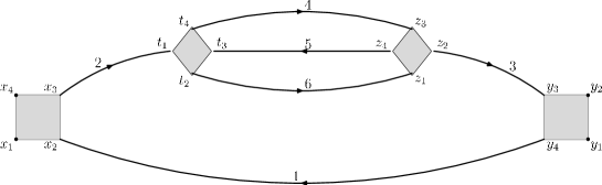
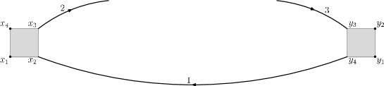
In the commutative case, this operation corresponds to the shrinking of $S$ to a point: it represents the ”Moyality" (instead of locality) of the theory.

E.2.2 Parametric representation for NCQFT

In this subsection we recall the definitions and results obtained in [39] for the parametric representations of the model defined by eq. (5.7). First let us recall that, when considering the parametric representation for commutative QFT, one has translation invariance in position space. As a consequence of this invariance, the first polynomial vanishes when integrating over all internal positions. Therefore, one has to integrate over all internal positions (which correspond to vertices) save one, which is thus marked. However, the polynomial is a still a canonical object, i. e. it does not depend of the choice of this particular vertex.

As stated in [39], in the non-commutative case translation invariance is lost (because of non-locality). Therefore, one can integrate over all internal positions and hypermomenta. However, in order to be able to recover the commutative limit, we also mark a particular vertex $\bar{V}$; we do not integrate on its associate hypermomenta $p_{\bar{V}}$. This particular vertex is the root vertex. Because there is no translation invariance, the polynomial does depend on on the choice of the root; however the leading ultraviolet terms do not.

We define the $(L\times 4)$-dimensional incidence matrix $\varepsilon^{V}$ for each of the vertices $V$. Since the graph is orientable (in the sense defined in subsection E.2.1 above) we can choose

$$\varepsilon_{\ell i}^{V}=(-1)^{i+1},\mbox{ if the line $\ell$ hooks to the vertex $V$ at corner $i$.}$$ (5.12)

Let also

$$\eta^{V}_{\ell i}=|\varepsilon^{V}_{\ell i}|,\mbox{ }V=1,\ldots,n,\,\ell=1,\ldots,L\mbox{ and }i=1,\ldots,4.$$ (5.13)

From eq . (5.12) and (5.13) one has

$$\eta^{V}_{\ell i}=(-1)^{i+1}\varepsilon_{\ell i}.$$ (5.14)

We introduce withe the ”short" $u$ and ”long" $v$ variables by

$$v_{\ell} = \frac{1}{\sqrt{2}}\sum_{V}\sum_{i}\eta^{V}_{\ell i}x^{V}_{i},$$

$$u_{\ell} = \frac{1}{\sqrt{2}}\sum_{V}\sum_{i}\varepsilon^{V}_{\ell i}x^{V}_{i}.$$ (5.15)

Conversely, one has

$$x^{V}_{i}=\frac{1}{\sqrt{2}}\left(\eta^{V}_{\ell i}v_{\ell}+\varepsilon^{V}_{\ell i}u_{\ell}\right).$$ (5.16)

From the propagator 5.8 and vertices contributions 5.9 one is able to write the amplitude ${\cal A}_{G,{\bar{V}}}$ of the graph $G$ (with the marked root $\bar{V}$) in terms of the non-commutative polynomials $HU_{G,\bar{V}}$ and $HV_{G,\bar{V}}$ as (see [39] for details)

$${\cal A}_{G,{\bar{V}}}(x_{e},\;p_{\bar{V}})=\left(\frac{\tilde{\Omega}}{2^{\frac{D}{2}-1}}\right)^{L}\int_{0}^{\infty}\prod_{\ell=1}^{L}[dt_{\ell}(1-t_{\ell}^{2})^{\frac{D}{2}-1}]\frac{e^{-\frac{HV_{G,\bar{V}}(t_{\ell},x_{e},p_{\bar{v}})}{HU_{G,\bar{V}}(t)}}}{HU_{G,\bar{V}}(t)^{\frac{D}{2}}},$$ (5.17)

with $x_{e}$ the external positions of the graph and

$$t_{\ell}={\rm tanh}\frac{\alpha_{\ell}}{2},\ \ell=1,\ldots,L.$$ (5.18)

where $\alpha_{\ell}$ are the parameters associated by eq. (5.8) to the propagators of the graph. In [39] it was proved that $HU$ and $HV$ are polynomials in the set of variables $t$. The first polynomial is given by (see again [39])

$$HU_{G,\bar{V}}=({\rm det}Q)^{\frac{1}{D}}\prod_{\ell=1}^{L}t_{\ell}\,,$$ (5.19)

where

$$Q=A\otimes 1_{D}-B\otimes\sigma\,,$$ (5.20)

with $A$ a diagonal matrix and $B$ an antisymmetric matrix. The matrix $A$ writes

$$A=\begin{pmatrix}S&0&0\\ 0&T&0\\ 0&0&0\\ \end{pmatrix}\,,$$ (5.21)

where $S$ and resp. $T$ are the two diagonal $L$ by $L$ matrices with diagonal elements $c_{\ell}=\coth(\frac{\alpha_{\ell}}{2})=1/t_{\ell}$, and resp. $t_{\ell}$. The last $(n-1)$ lines and columns are have $0$ entries.

The antisymmetric part $B$ is

$$B=\begin{pmatrix}{s}E&C\\ -C^{t}&0\\ \end{pmatrix}\,,$$ (5.22)

with

$$s=\frac{2}{\theta\tilde{\Omega}}=\frac{1}{\Omega}\,,$$ (5.23)

and

$$C_{\ell V}=\begin{pmatrix}\sum_{i=1}^{4}(-1)^{i+1}\varepsilon^{V}_{\ell i}\\ \sum_{i=1}^{4}(-1)^{i+1}\eta^{V}_{\ell i}\\ \end{pmatrix}\ ,$$ (5.24)

$$E=\begin{pmatrix}E^{uu}&E^{uv}\\ E^{vu}&E^{vv}\\ \end{pmatrix}.$$ (5.25)

The blocks of the matrix $E$ are

$$E^{vv}_{\ell,\ell^{\prime}} = \sum_{V}\sum_{i,j=1}^{4}(-1)^{i+j+1}\omega(i,j)\eta_{\ell i}^{V}\eta_{\ell^{\prime}j}^{V},$$

$$E^{uu}_{\ell,\ell^{\prime}} = \sum_{V}\sum_{i,j=1}^{4}(-1)^{i+j+1}\omega(i,j)\varepsilon_{\ell i}^{V}\varepsilon_{\ell^{\prime}j}^{V},$$

$$E^{uv}_{\ell,\ell^{\prime}} = \sum_{V}\sum_{i,j=1}^{4}(-1)^{i+j+1}\omega(i,j)\varepsilon_{\ell i}^{V}\eta_{\ell^{\prime}j}^{V}.$$ (5.26)

The symbol $\omega(i,j)$ takes the values $\omega(i,j)=1$ if $i<j$, $\omega(i,j)=-1$ is $j<i$ and $\omega(i,j)=0$ if $i=j$. In eq. (5.24) of the matrix $C$ we have rescaled by $s$ the hypermomenta $p_{V}$. For further reference we introduce the integer entries matrix:

$$B^{\prime}=\begin{pmatrix}E&C\\ -C^{t}&0\\ \end{pmatrix}\ .$$ (5.27)

In [39] it was proven that

$${\rm det}Q=({\rm det}M)^{D}\,,$$ (5.28)

where

$$M=A+B\,.$$ (5.29)

Thus eq. (5.19) becomes:

$$HU_{G,\bar{V}}={\rm det}M\prod_{\ell=1}^{L}t_{\ell}\,.$$ (5.30)

Let $I$ and resp. $J$ be two subsets of $\{1,\ldots,L\}$, of cardinal $|I|$ and $|J|$. Let

$$k_{I,J}=|I|+|J|-L-F+1\,,$$ (5.31)

and $n_{IJ}=\mathrm{Pf}(B^{\prime}_{\hat{I}\hat{J}})$, the Pffafian of the matrix $B^{\prime}$ with deleted lines and columns $I$ among the first $L$ indices (corresponding to short variables $u$) and $J$ among the next $L$ indices (corresponding to long variables $v$).

The specific form 5.21 allows one to write the polynomial $HU$ as a sum of positive terms:

$$HU_{G,{\bar{V}}}(t) = \sum_{I,J}s^{2g-k_{I,J}}\ n_{I,J}^{2}\prod_{\ell\not\in I}t_{\ell}\prod_{\ell^{\prime}\in J}t_{\ell^{\prime}}\ .$$ (5.32)

In [39], non-zero leading terms (i. e. terms with the smallest global degree in the $t$ variables) were identified. These terms are dominant in the UV regime. Some of them correspond to subsets $I=\{1,\ldots,L\}$ and $J$ admissible, that is

• $J$ contains a tree $\tilde{\cal T}$ in the dual graph,

• the complement of $J$ contains a tree $\cal T$ in the direct graph.

Associated to such $I$ and $J$ one has $n_{I,J}^{2}=2^{2g}$.

However, the list of these leading terms, as already remarked in [39], is not exhaustive. In the next section we complete this list with further terms, necessary for the sequel .

We end this section with the explicit example of the bubble and the sunshine graph (Fig. E.7 and Fig. E.8).

Figure E.7: The bubble graph

For the bubble graph one has

$$HU_{G,\bar{V}} = (1+4s^{2})(t_{1}+t_{2}+t_{1}^{2}t_{2}+t_{1}t_{2}^{2}).$$ (5.33)

Figure E.8: The sunshine graph

For the sunshine graph one has

$$HU_{G,\bar{V}} = \Big{[}t_{1}t_{2}+t_{1}t_{3}+t_{2}t_{3}+t_{1}^{2}t_{2}t_{3}+t_{1}t_{2}^{2}t_{3}+t_{1}t_{2}t_{3}^{2}\Big{]}(1+4s^{2})^{2}$$ (5.34)

$$+16s^{2}(t_{2}^{2}+t_{1}^{2}t_{3}^{2}).$$

For further reference we also give the polynomial of the graph of Fig. E.6

$$HU_{G,\bar{V}}=(1+4s^{2})(t_{1}+t_{2}+t_{3}+t_{1}t_{2}t_{3})(1+t_{2}t_{3}+t_{1}(t_{2}+t_{3})).$$ (5.35)

The polynomial $HV$ is more involved. One has

$$\frac{HV_{G,\bar{V}}}{HU_{G,\bar{V}}}=\frac{\tilde{\Omega}}{2}\begin{pmatrix}x_{e}&p_{\bar{V}}\end{pmatrix}PQ^{-1}P^{t}\begin{pmatrix}x_{e}\\ p_{\bar{V}}\end{pmatrix},$$ (5.36)

where $P$ is some matrix coupling the external positions $x_{e}$ and the root hypermomenta $p_{\bar{V}}$ with the short $u$ and long $v$ variables and the rest of the hypermomenta $p_{V}$ ($V\neq\bar{V}$). Explicit expressions can be found in [39].

E.3 Further leading terms in HU

To procede with the dimensional regularization one needs first to correctly isolate the divergent subgraphs in different Hepp sectors. Let a subgraph $S$ in the graph G. If $S$ is nonplanar the leading terms in $HU_{G}$ suffice to prove that $S$ is convergent in every Hepp sector as will be explained in section E.5.

This is not the case if $S$ is planar with more that one broken face. Let $\tilde{\ell}$ be the line of $G$ which breaks an internal face of $S$.

If $\tilde{\ell}$ is a genus line in $G$ (see subsection E.2.1), one could still use only the leading terms in $HU_{G}$ to prove that $S$ is convergent.

But one still needs to prove that $S$ is convergent if the line $\tilde{\ell}$ is not a genus line in $G$. This is for instance the case of the sunshine graph: in the Hepp sector $t_{1}<t_{3}<t_{2}$ one must prove that the subgraph formed by the lines $l_{1}$ and $l_{3}$ is convergent. This is true due to the term $16s^{2}t_{2}^{2}$ in eq. (5.34). Note that the variable $t_{2}$ is associated to the line which breaks the internal face of the subgraph $\ell_{1}$, $\ell_{3}$. One needs to prove that for arbitrary $G$ and $S$ we have such terms.

If we reduce $S$ to a rosette there exists a loop line $\ell_{2}\in S$ which either crosses $\tilde{\ell}$ or encompasses it. This line separates the two broken faces of $S$.

Definition E.3.1

Let $J_{0}$ a subset of the internal lines of the graph $G$. $J_{0}$ is called pseudo-admissible if:

• its complement is the union of tree $\cal T$ in $G$ and $\ell_{2}$,

• neither $\tilde{\ell}$ nor $\ell_{2}$ belong to $\cal T$,

Let $I_{0}=\{\ell_{1}\ldots\ell_{L}\}-\tilde{\ell}\equiv I-\tilde{\ell}$. This implies $|I|=L(G)-1$ and $|J|=F(G)-2+2g(G)$. For the sunshine graph (see Fig. E.8) $I=\{\ell_{1},\ell_{3}\}$ and $J=\{\ell_{2}\}$. One has the theorem

Theorem E.3.1

In the sum 5.32 the term associated to $I_{0}$ and $J_{0}$ above is

$$n_{I_{0},J_{0}}^{2} = 4,\mbox{ if $\tilde{\ell}$ is a genus line, in $G$}$$

$$= 16,\mbox{ if $\tilde{\ell}$ is not a genus line in $G$.}$$

Proof: The proof is similar to the one concerning the leading terms of $HU$ given in Lemma $III.1$ of [39], being however more involved.

The matrix whose determinant we must compute is obtained from $B$ by deleting the lines and columns corresponding to the subsets $I_{0}$ and $J_{0}$ (as explained in the previous section).

The matrix $B^{\prime}_{\hat{I}_{0},\hat{J}_{0}}$ has

• a line and column corresponding to $u_{\tilde{\ell}}$, the short variable of $\tilde{\ell}$

• $n$ lines and columns corresponding to the $v$ variables of the $n-1$ tree lines of $\cal T$ and the supplementary line $\ell_{2}$

• $n-1$ lines and columns associated to the hypermomenta.

We represent the determinant of this matrix by the Grassmann integral:

$${\rm det}B^{\prime}_{\hat{I}_{0},\hat{J}_{0}}=\int d\bar{\psi}^{u}_{\tilde{\ell}}d\psi^{u}_{\tilde{\ell}}d\bar{\psi}^{v}d\psi^{v}d\bar{\psi}^{p}d\psi^{p}e^{-\bar{\psi}B^{\prime}\psi}$$ (5.1)

The quadratic form in the Grassman variables in the above integral is:

$$-\sum_{V}\sum_{l;i,j}\bar{\psi}^{u}_{\tilde{\ell}}(-1)^{i+1}\omega(i,j)\varepsilon^{V}_{\tilde{\ell}i}\varepsilon^{V}_{\ell j}\psi^{v}_{\ell}$$ (5.2)

$$-\sum_{V}\sum_{l;i,j}\bar{\psi}^{v}_{\ell}\omega(i,j)\varepsilon^{V}_{\ell i}\varepsilon^{V}_{\tilde{\ell}j}(-1)^{j+1}\psi^{u}_{\tilde{\ell}}$$

$$+\sum_{V}\bar{\psi}^{u}_{\tilde{\ell}}(-1)^{i+1}\varepsilon^{V}_{\tilde{\ell}i}\psi^{p_{V}}-\sum_{V}\bar{\psi}^{p_{V}}(-1)^{i+1}\varepsilon^{V}_{\tilde{\ell}i}\psi^{u}_{\tilde{\ell}}$$

$$-\sum_{V}\sum_{\ell,\ell^{\prime};i,j}\bar{\psi}^{v}_{\ell}\omega(i,j)\varepsilon^{V}_{\ell i}\varepsilon^{V}_{\ell^{\prime}j}\psi^{v}_{\ell^{\prime}}$$

$$+\sum_{V}\sum_{\ell;i}\bar{\psi}^{v}_{\ell}\varepsilon^{V}_{\ell i}\psi^{p_{V}}-\sum_{V}\sum_{\ell;i}\bar{\psi}^{p_{V}}\varepsilon^{V}_{\ell i}\psi^{v}_{\ell}\,.$$

We implement the first Filk move as a Grasmann change of variales. At each step we reduce a tree line $\ell_{1}=(i,j)$ connecting the root vertex $\bar{V}_{G}$ to a normal vertex $V$ and gluing the two vertices. This is achieved by performing a change of variables for the hypermomenta and reinterpreting the quadratic form in the new variables as corresponding to a new vertex $\bar{V}^{\prime}_{G}$: the quadratic form essentially reproduces itself under the change of variables!

Take $\ell_{1}=(i,j)$ a line connecting the ”root" vertex $\bar{V}_{G}$ to a vertex $V$. We make the change of variables

$$\psi^{p_{V}} = \chi^{p_{V}}+\sum_{\ell^{\prime}\neq\ell_{1}}\sum_{k}\left(-\omega(i,k)\varepsilon^{\bar{V}_{G}}_{\ell^{\prime}k}+\omega(j,k)\varepsilon^{V}_{\ell^{\prime}k}\right)\psi^{v}_{\ell^{\prime}}$$

$$+\sum_{k}\left(-\omega(i,k)\varepsilon^{\bar{V}_{G}}_{\tilde{\ell}k}+\omega(j,k)\varepsilon^{V}_{\tilde{\ell}k}\right)(-1)^{k+1}\psi^{u}_{\tilde{\ell}}$$

$$\bar{\psi}^{p_{V}} = \bar{\chi}^{p_{V}}+\sum_{\ell^{\prime}\neq\ell_{1}}\sum_{k}\left(-\omega(i,k)\varepsilon^{\bar{V}_{G}}_{\ell^{\prime}k}+\omega(j,k)\varepsilon^{V}_{\ell^{\prime}k}\right)\bar{\psi}^{v}_{\ell^{\prime}}$$ (5.3)

$$+\sum_{k}\left(-\omega(i,k)\varepsilon^{\bar{V}_{G}}_{\tilde{\ell}k}+\omega(j,k)\varepsilon^{V}_{\tilde{\ell}k}\right)(-1)^{k+1}\bar{\psi}^{u}_{\tilde{\ell}}\,,$$

where the first sum is performed on the internal lines of $G$ (note that because of the presence of the incidences matrices $\varepsilon$ this sum reduces to a sum on the lines hooked to the two vertices $\bar{V}_{G}$ and $V$). The corners $i$ and resp. $j$ are the corners where the tree line $\ell_{1}$ hooks to the vertex $\bar{V}_{G}$ and resp. $V$.

At each step, let us consider the coupling between the variables associated to the line $\ell_{1}$ and to the hypermomentum $p_{V}$ and the rest of the variables. Using eq. (5.2) one has

$$-\bar{\psi}^{u}_{\tilde{\ell}}\sum_{p}(-1)^{p+1}\left(\omega(p,i)\varepsilon^{V_{G}}_{\tilde{\ell}p}\varepsilon^{V_{G}}_{\ell_{1}i}+\omega(p,j)\varepsilon^{V}_{\tilde{\ell}p}\varepsilon^{V}_{\ell_{1}j}\right)\psi^{v}_{\ell_{1}}$$

$$-\bar{\psi}^{v}_{\ell_{1}}\sum_{p}\left(\omega(i,p)\varepsilon^{V_{G}}_{\tilde{\ell}p}\varepsilon^{V_{G}}_{\ell_{1}i}+\omega(j,p)\varepsilon^{V}_{\tilde{\ell}p}\varepsilon^{V}_{\ell_{1}j}\right)\psi^{u}_{\tilde{\ell}}(-1)^{p+1}$$

$$+\sum_{V;p}\bar{\psi}^{u}_{\tilde{\ell}}(-1)^{p+1}\varepsilon^{V}_{\tilde{\ell}p}\psi^{p_{V}}-\sum_{V;p}\bar{\psi}^{p_{V}}(-1)^{p+1}\varepsilon^{V}_{\tilde{\ell}p}\psi^{u}_{\tilde{\ell}}$$

$$-\bar{\psi}^{v}_{\ell_{1}}\sum_{\ell^{\prime}\neq\ell_{1};k}\left(\omega(i,k)\varepsilon^{\bar{V}_{G}}_{\ell_{1}i}\varepsilon^{\bar{V}_{G}}_{\ell^{\prime}k}+\omega(j,k)\varepsilon^{V}_{\ell_{1}j}\varepsilon^{V}_{\ell^{\prime}k}\right)\psi^{v}_{\ell^{\prime}}$$

$$-\sum_{\ell^{\prime}\neq\ell_{1};k}\bar{\psi}^{v}_{\ell^{\prime}}\left(\omega(k,i)\varepsilon^{\bar{V}_{G}}_{\ell^{\prime}k}\varepsilon^{\bar{V}_{G}}_{\ell_{1}i}+\omega(k,j)\varepsilon^{V}_{\ell^{\prime}k}\varepsilon^{V}_{\ell_{1}j}\right)\psi^{v}_{\ell_{1}}$$

$$+\bar{\psi}^{v}_{\ell_{1}}\varepsilon^{V}_{\ell_{1}j}\psi^{p_{V}}+\sum_{\ell^{\prime}\neq\ell_{1};k}\bar{\psi}^{v}_{\ell^{\prime}}\varepsilon^{V}_{\ell^{\prime}k}\psi^{p_{V}}$$

$$-\bar{\psi}^{p_{V}}\varepsilon^{V}_{\ell_{1}j}\psi^{v}_{\ell}-\sum_{\ell^{\prime}\neq\ell_{1};k}\bar{\psi}^{p_{V}}\varepsilon^{V}_{\ell^{\prime}k}\psi^{v}_{\ell^{\prime}}\,,$$ (5.4)

which rewrites as

$$-\Big{[}\bar{\psi}^{u}_{\tilde{\ell}}\sum_{p}(-1)^{p+1}\left(\omega(p,i)\varepsilon^{V_{G}}_{\tilde{\ell}p}\varepsilon^{V_{G}}_{\ell_{1}i}+\omega(p,j)\varepsilon^{V}_{\tilde{\ell}p}\varepsilon^{V}_{\ell_{1}j}\right)$$

$$+\sum_{\ell^{\prime}\neq\ell_{1};k}\bar{\psi}^{v}_{\ell^{\prime}}\left(\omega(k,i)\varepsilon^{\bar{V}_{G}}_{\ell^{\prime}k}\varepsilon^{\bar{V}_{G}}_{\ell_{1}i}+\omega(k,j)\varepsilon^{V}_{\ell^{\prime}k}\varepsilon^{V}_{\ell_{1}j}\right)+\bar{\psi}^{p_{V}}\varepsilon^{V}_{\ell_{1}j}\Big{]}\psi^{v}_{\ell_{1}}$$

$$-\bar{\psi}^{v}_{\ell_{1}}\Big{[}\sum_{p}\left(\omega(i,p)\varepsilon^{V_{G}}_{\tilde{\ell}p}\varepsilon^{V_{G}}_{\ell_{1}i}+\omega(j,p)\varepsilon^{V}_{\tilde{\ell}p}\varepsilon^{V}_{\ell_{1}j}\right)\psi^{u}_{\tilde{\ell}}(-1)^{p+1}$$

$$+\sum_{\ell^{\prime}\neq\ell_{1};k}\left(\omega(i,k)\varepsilon^{\bar{V}_{G}}_{\ell_{1}i}\varepsilon^{\bar{V}_{G}}_{\ell^{\prime}k}+\omega(j,k)\varepsilon^{V}_{\ell_{1}j}\varepsilon^{V}_{\ell^{\prime}k}\right)\psi^{v}_{\ell^{\prime}}-\varepsilon^{V}_{\ell_{1}j}\psi^{p_{V}}\Big{]}$$

$$+\sum_{V;p}\bar{\psi}^{u}_{\tilde{\ell}}(-1)^{p+1}\varepsilon^{V}_{\tilde{\ell}p}\psi^{p_{V}}-\sum_{V;p}\bar{\psi}^{p_{V}}(-1)^{p+1}\varepsilon^{V}_{\tilde{\ell}p}\psi^{u}_{\tilde{\ell}}$$

$$+\sum_{\ell^{\prime}\neq\ell_{1};k}\bar{\psi}^{v}_{\ell^{\prime}}\varepsilon^{V}_{\ell^{\prime}k}\psi^{p_{V}}-\sum_{\ell^{\prime}\neq\ell_{1};k}\bar{\psi}^{p_{V}}\varepsilon^{V}_{\ell^{\prime}k}\psi^{v}_{\ell^{\prime}}\,.$$ (5.5)

Performing now in E.3 the change of variable E.3 for the hypermomentum $p_{V}$ of the vertex $V$ associated to the tree line $\ell_{1}$ of $G$ and taking into account that $\varepsilon_{\ell_{1}i}=-\varepsilon_{\ell_{1}j}$ the first two lines of E.3 are simply

$$-\bar{\chi}^{p_{V}}\varepsilon^{V}_{\ell_{1}j}\psi^{v}_{\ell_{1}}+\bar{\psi}^{v}_{\ell_{1}}\varepsilon^{V}_{\ell_{1}j}\chi^{p_{V}}\,.$$ (5.6)

As $\psi^{v}_{\ell_{1}}$ and $\bar{\psi}^{v}_{\ell_{1}}$ do not appear anymore in the rest of the terms we are forced to pair them with $\bar{\chi}^{p_{V}}$ and $\chi^{p_{V}}$. The rest of the terms in the quadratic form are:

$$+\sum_{V;p}\bar{\psi}^{u}_{\tilde{\ell}}(-1)^{p+1}\varepsilon^{V}_{\tilde{\ell}p}\Big{[}\sum_{\ell^{\prime}\neq\ell_{1}}\sum_{k}\left(-\omega(i,k)\varepsilon^{\bar{V}_{G}}_{\ell^{\prime}k}+\omega(j,k)\varepsilon^{V}_{\ell^{\prime}k}\right)\psi^{v}_{\ell^{\prime}}$$

$$+\sum_{k}\left(-\omega(i,k)\varepsilon^{\bar{V}_{G}}_{\tilde{\ell}k}+\omega(j,k)\varepsilon^{V}_{\tilde{\ell}k}\right)(-1)^{k+1}\psi^{u}_{\tilde{\ell}}\Big{]}$$

$$+\sum_{\ell^{\prime}\neq\ell_{1};p}\bar{\psi}^{v}_{\ell^{\prime}}\varepsilon^{V}_{\ell^{\prime}p}\Big{[}\sum_{\ell^{\prime}\neq\ell_{1}}\sum_{k}\left(-\omega(i,k)\varepsilon^{\bar{V}_{G}}_{\ell^{\prime}k}+\omega(j,k)\varepsilon^{V}_{\ell^{\prime}k}\right)\psi^{v}_{\ell^{\prime}}$$

$$+\sum_{k}\left(-\omega(i,k)\varepsilon^{\bar{V}_{G}}_{\tilde{\ell}k}+\omega(j,k)\varepsilon^{V}_{\tilde{\ell}k}\right)(-1)^{k+1}\psi^{u}_{\tilde{\ell}}\Big{]}$$

$$-\sum_{V;p}\Big{[}\sum_{\ell^{\prime}\neq\ell_{1}}\sum_{k}\left(-\omega(i,k)\varepsilon^{\bar{V}_{G}}_{\ell^{\prime}k}+\omega(j,k)\varepsilon^{V}_{\ell^{\prime}k}\right)\bar{\psi}^{v}_{\ell^{\prime}}$$

$$+\sum_{k}\left(-\omega(i,k)\varepsilon^{\bar{V}_{G}}_{\tilde{\ell}k}+\omega(j,k)\varepsilon^{V}_{\tilde{\ell}k}\right)(-1)^{k+1}\bar{\psi}^{u}_{\tilde{\ell}}\Big{]}(-1)^{p+1}\varepsilon^{V}_{\tilde{\ell}p}\psi^{u}_{\tilde{\ell}}$$

$$-\Big{[}\sum_{\ell^{\prime}\neq\ell_{1}}\sum_{k}\left(-\omega(i,k)\varepsilon^{\bar{V}_{G}}_{\ell^{\prime}k}+\omega(j,k)\varepsilon^{V}_{\ell^{\prime}k}\right)\bar{\psi}^{v}_{\ell^{\prime}}$$

$$+\sum_{k}\left(-\omega(i,k)\varepsilon^{\bar{V}_{G}}_{\tilde{\ell}k}+\omega(j,k)\varepsilon^{V}_{\tilde{\ell}k}\right)(-1)^{k+1}\bar{\psi}^{u}_{\tilde{\ell}}\Big{]}\sum_{\ell^{\prime}\neq\ell_{1};p}\varepsilon^{V}_{\ell^{\prime}p}\psi^{v}_{\ell^{\prime}}\;.$$ (5.7)

We analyse the different terms in the above equation. The term $\bar{\psi}^{u}_{\tilde{\ell}}\psi^{u}_{\tilde{\ell}}$ is:

$$\sum_{p,k}\varepsilon^{V}_{\tilde{\ell}p}(-1)^{p+1}\Big{[}-\omega(i,k)\varepsilon^{\bar{V}_{G}}_{\tilde{\ell}k}+\omega(j,k)\varepsilon^{V}_{\tilde{\ell}k}\Big{]}(-1)^{k+1}$$

$$-\sum_{p,k}\Big{[}-\omega(i,k)\varepsilon^{\bar{V}_{G}}_{\tilde{\ell}k}+\omega(j,k)\varepsilon^{V}_{\tilde{\ell}k}\Big{]}(-1)^{k+1}\varepsilon^{V}_{\tilde{\ell}p}(-1)^{p+1}=0\,.$$ (5.8)

The term in $\bar{\psi}^{u}_{\tilde{\ell}}\psi^{v}_{\ell^{\prime}}$ is given by:

$$+\sum_{p}\bar{\psi}^{u}_{\tilde{\ell}}(-1)^{p+1}\varepsilon^{V}_{\tilde{\ell}p}\sum_{\ell^{\prime}\neq\ell_{1}}\sum_{k}\left(-\omega(i,k)\varepsilon^{\bar{V}_{G}}_{\ell^{\prime}k}+\omega(j,k)\varepsilon^{V}_{\ell^{\prime}k}\right)\psi^{v}_{\ell^{\prime}}$$

$$-\sum_{p}\left(-\omega(i,p)\varepsilon^{\bar{V}_{G}}_{\tilde{\ell}p}+\omega(j,p)\varepsilon^{V}_{\tilde{\ell}p}\right)(-1)^{p+1}\bar{\psi}^{u}_{\tilde{\ell}}\sum_{\ell^{\prime}\neq\ell_{1};k}\varepsilon^{V}_{\ell^{\prime}k}\psi^{v}_{\ell^{\prime}}\,.$$ (5.9)

Setting $j$ to be either the first or the last halfline on the vertex $V$ we see that the last terms in the two lines above cancel eachother. The first two terms hold:

$$\sum_{p}\sum_{\ell^{\prime}\neq\ell_{1}}\sum_{k}\bar{\psi}^{u}_{\tilde{\ell}}\psi^{v}_{\ell^{\prime}}(-1)^{p+1}\Big{[}-\omega(i,k)\varepsilon^{\bar{V}_{G}}_{\ell^{\prime}k}\varepsilon^{V}_{\tilde{\ell}p}+\omega(i,p)\varepsilon^{\bar{V}_{G}}_{\tilde{\ell}p}\varepsilon^{V}_{\ell^{\prime}k}\Big{]}\,.$$ (5.10)

This can be rewritten in the form:

$$-\sum_{p}\sum_{\ell^{\prime}\neq\ell_{1}}\sum_{k}\bar{\psi}^{u}_{\tilde{\ell}}\psi^{v}_{\ell^{\prime}}(-1)^{p+1}\omega(p,k)\varepsilon_{\tilde{\ell}p}^{\bar{V}_{G}^{\prime}}\varepsilon_{\ell^{\prime}k}^{\bar{V}_{G}^{\prime}}\,,$$ (5.11)

where $\bar{V}_{G}^{\prime}$ is a new root vertex in which the vertex $V$ has been glued to the vertex $\bar{V}_{G}$ and the halflines on the vertex $V$ have been inserted on the new vertex at the place of the halfline $i$.

The coupling between $\psi^{v}$’s with $\psi^{v}$’is

$$+ \sum_{\ell\neq\ell_{1},k}\bar{\psi}^{v}_{\ell}\varepsilon^{V}_{\ell k}\sum_{\ell^{\prime}}\left(-\sum_{p}\varepsilon^{\bar{V}_{G}}_{\ell^{\prime}p}\omega(i,p)+\sum_{k^{\prime}=1}^{4}\varepsilon^{V}_{\ell^{\prime}k^{\prime}}\omega(j,k^{\prime})\right)\psi^{v}_{\ell^{\prime}}$$ (5.12)

$$- \sum_{\ell^{\prime}\neq\ell_{1}}\left(-\sum_{p}\varepsilon^{\bar{V}_{G}}_{\ell^{\prime}p}\omega(i,p)+\sum_{k=1}^{4}\varepsilon^{V}_{\ell^{\prime}k}\omega(j,k)\right)\bar{\psi}^{v}_{\ell^{\prime}}\sum_{\ell\neq\ell_{1};k^{\prime}}\varepsilon^{V}_{\ell k^{\prime}}\psi^{v}_{\ell}\ .$$

Again, as $j$ is either the first or the last halfline on the vertex $V$, the last two terms in the two lines of eq. (5.12) cancel each other. The rest of the terms give exactly the contacts between the $\bar{\psi}^{v}$ and $\psi^{v}$ on a new vertex $\bar{V}_{G}^{\prime}$ obtained by gluing $V$ on $\bar{V}_{G}$ This is the first Filk move on the line $\ell_{1}$ and its associated vertex $V$. One iterates now this mechanism for the rest of the tree lines of $G$. Hence we reduce the graph $G$ to a rosette (see subsection E.2.1).

The quadratic form writes finally as

$$-\sum_{\ell^{\prime};p,k}\bar{\psi}^{u}_{\tilde{\ell}}\psi^{v}_{\ell^{\prime}}(-1)^{p+1}\omega(p,k)\varepsilon_{\tilde{\ell}p}^{\bar{V}_{G}}\varepsilon_{\ell^{\prime}k}^{\bar{V}_{G}}-\sum_{\ell^{\prime};p,k}\bar{\psi}^{v}_{\ell^{\prime}}\psi^{u}_{\tilde{\ell}}(-1)^{p+1}\omega(k,p)\varepsilon_{\tilde{\ell}p}^{\bar{V}_{G}}\varepsilon_{\ell^{\prime}k}^{\bar{V}_{G}}$$

$$-\sum_{\ell,\ell^{\prime};j,k}\bar{\psi}^{v}_{\ell}\varepsilon^{\bar{V}_{G}}_{\ell j}\varepsilon^{\bar{V}_{G}}_{\ell^{\prime}k}\omega(j,k)\psi^{v}_{\ell^{\prime}}\,.$$ (5.13)

The sum concerns only the rosette vertex $\bar{V}_{G}$. Therefore the last line is $0$, as by the first Filk move we have exhausted all the tree lines of $\cal T$.

As $\tilde{\ell}$ breaks the face separated from the external face by $\ell_{2}$ we have $k_{1}<p<k_{2}$. By a direct inspection of the terms above, one obtains the requested result.

$\Box$

E.4 Factorization of the Feynman amplitudes

Take now $S$ to be a primitively divergent subgraph. We now prove that the Feynman amplitude ${\cal A}_{G}$ factorizes into two parts, one corresponding to the primitive divergent subgraph $S$ and the other to the graph $G/S$ (defined in section E.2.1). This is needed in order to prove that divergencies are cured by Moyal counterterms .

In section E.5 we will prove that only the planar ($g=0$), one broken face $B=1$, $N=2$ or $N=4$ external legs subgraphs are primitively divergent. We now deal only with such subgraphs.

E.4.1 Factorization of the polynomial $HU$

We denote all the leading terms in the first polynomial associated to a graph $S$ by $HU^{l}_{S}$. If we rescale all the $t_{\ell}$ parameters corresponding to a subgraph $S$ by $\rho^{2}$, $HU_{G}$ becomes a polynomial in $\rho$. We denote the terms of minimal degree in $\rho$ in this polynomial by $HU_{G}^{l(\rho)}$. It is easy to see that for the subgraph $S$ we have $HU^{l(\rho)}_{S}=\rho^{2[L(S)-n(S)+1]}HU^{l}_{S}|_{\rho=1}$. We have the following theorem

Theorem E.4.1

Under the rescaling

$$t_{\alpha}\mapsto\rho^{2}t_{\alpha}$$ (5.1)

of the parameter corresponding to a divergent subgraph $S$ of any Feynman graph $G$, the following factorization property holds

$$HU^{l(\rho)}_{G,\bar{V}}=HU^{l(\rho)}_{S,\bar{V}_{S}}HU_{G/S,\bar{V}}\;.$$ (5.2)

Proof:
In the matrix $M$ defined in eq. (5.29) (corresponding to the graph $G$) we can rearrange the lines and columns so that we place the matrix $M_{S}$ (corresponding to the subgraph $S$) into the upper left corner. We place the line (and resp. the column) associated to the hypermomentum of the root vertex of $S$ to be the last line (and resp. column) of $M$ (without loss of generality we consider that the root of the subgraph $S$ is not the root of $G$). $M$ takes the form

$$\hskip-5.69046pt\begin{pmatrix}E^{u^{S}u^{S}}&E^{u^{S}v^{S}}&C^{u^{S}p^{S}}&E^{u^{S}u^{G-S}}&E^{u^{S}v^{G-S}}&C^{u^{S}p^{G-S}}\\ E^{v^{S}u^{S}}&E^{v^{S}v^{S}}&C^{v^{S}p^{S}}&E^{v^{S}u^{G-S}}&E^{v^{S}v^{G-S}}&C^{v^{S}p^{G-S}}\\ C^{p^{S}u^{S}}&C^{p^{S}v^{S}}&0&C^{p^{S}u^{G-S}}&C^{p^{S}v^{G-S}}&0\\ E^{u^{G-S}u^{S}}&E^{u^{G-S}v^{S}}&C^{u^{G-S}p^{S}}&E^{u^{G-S}u^{G-S}}&E^{u^{G-S}v^{G-S}}&C^{u^{G-S}p^{G-S}}\\ E^{v^{G-S}u^{S}}&E^{v^{G-S}v^{S}}&C^{v^{G-S}p^{S}}&E^{v^{G-S}u^{G-S}}&E^{v^{G-S}v^{G-S}}&C^{v^{G-S}p^{G-S}}\\ C^{p^{G-S}u^{S}}&C^{p^{G-S}v^{S}}&0&C^{p^{G-S}u^{G-S}}&C^{p^{G-S}v^{G-S}}&0\end{pmatrix}$$

where we have denoted by $E^{u^{S}u^{S}}$ a coupling between two short variables corresponding to internal lines of $S$ etc..

I. We first write the determinant of the matrix above under the form of a Grassmannian integral

$${\rm det}M=\int d\bar{\psi}^{u}d\psi^{u}d\bar{\psi}^{v}d\psi^{v}d\bar{\psi}^{p}d\psi^{p}e^{-\bar{\psi}M\psi}\,.$$ (5.3)

Denote a generic line of the subgraph $S$ by $\ell_{S}$ and a generig line of the subgraph $G-S$ by $\ell_{G-S}$.

We perform a Grassmann change of variables of Jacobian $1$. The value of the integral (5.3) does not change under this change of variables. We will prove that the following properties hold for the different terms in the Grassmanian quadratic form

$$E^{\prime v^{S}v^{S}}=\mathrm{diag}(t_{l}),\quad E^{\prime v^{S}u^{G-S}}=0,\quad E^{\prime v^{S}v^{G-S}}=0$$ (5.4)

$$E^{\prime u^{G-S}u^{G-S}}=E^{\prime u^{G/S}u^{G/S}},\quad E^{\prime u^{G-S}v^{G-S}}=E^{\prime u^{G/S}v^{G/S}}$$

$$E^{\prime v^{G-S}v^{G-S}}=E^{\prime v^{G/S}v^{G/S}}.$$

The new matrix of the quadratic form $M^{\prime}$will now be

$$\hskip-5.69046pt\begin{pmatrix}E^{\prime u^{S}u^{S}}&E^{\prime u^{S}v^{S}}&C^{u^{S}p^{S}}&E^{\prime u^{S}u^{G-S}}&E^{\prime u^{S}v^{G-S}}&C^{u^{S}p^{G-S}}\\ E^{\prime v^{S}u^{S}}&E^{\prime v^{S}v^{S}}&C^{v^{S}p^{S}}&0&0&C^{v^{S}p^{G-S}}\\ C^{p^{S}u^{S}}&C^{p^{S}v^{S}}&0&C^{p^{S}u^{G-S}}&C^{p^{S}v^{G-S}}&0\\ E^{\prime u^{G-S}u^{S}}&0&C^{u^{G-S}p^{S}}&E^{\prime u^{G/S}u^{G/S}}&E^{\prime u^{G/S}v^{G/S}}&C^{u^{G-S}p^{G-S}}\\ E^{\prime v^{G-S}u^{S}}&0&C^{v^{G-S}p^{S}}&E^{\prime v^{G/S}u^{G/S}}&E^{\prime v^{G/S}v^{G/S}}&C^{v^{G-S}p^{G-S}}\\ C^{p^{G-S}u^{S}}&C^{p^{G-S}v^{S}}&0&C^{p^{G-S}u^{G-S}}&C^{p^{G-S}v^{G-S}}&0\end{pmatrix}$$

The first part of the proof follows that of section E.3, where we replace

$$\psi^{u}_{\tilde{\ell}}\rightarrow\sum_{\ell^{\prime}\in G-S}\psi^{u}_{\ell^{\prime}}\qquad\bar{\psi}^{u}_{\tilde{\ell}}\rightarrow\sum_{\ell^{\prime}\in G-S}\bar{\psi}^{u}_{\ell^{\prime}}\,.$$ (5.5)

Thus the appropriate change of variables is now

$$\psi^{p_{V}} = \chi^{p_{V}}+\sum_{\ell^{\prime}\neq\ell_{1};k}\left(-\omega(i,k)\varepsilon^{\bar{V}_{S}}_{\ell^{\prime}k}+\omega(j,k)\varepsilon^{V}_{\ell^{\prime};k}\right)\psi^{v}_{\ell^{\prime}}$$

$$+\sum_{\genfrac{}{}{0.0pt}{}{\ell^{\prime};k}{\ell^{\prime}\in G-S}}\left(-\omega(i,k)\varepsilon^{\bar{V}_{S}}_{\ell^{\prime}k}+\omega(j,k)\varepsilon^{V}_{\ell^{\prime}k}\right)(-1)^{k+1}\psi^{u}_{\ell^{\prime}}$$

$$\bar{\psi}^{p_{V}} = \bar{\chi}^{p_{V}}+\sum_{\ell^{\prime}\neq\ell_{1};k}\left(-\omega(i,k)\varepsilon^{\bar{V}_{S}}_{\ell^{\prime}k}+\omega(j,k)\varepsilon^{V}_{\ell^{\prime}k}\right)\bar{\psi}^{v}_{\ell^{\prime}}$$ (5.6)

$$+\sum_{\genfrac{}{}{0.0pt}{}{\ell^{\prime};k}{\ell^{\prime}\in G-S}}\left(-\omega(i,k)\varepsilon^{\bar{V}_{S}}_{\ell^{\prime}k}+\omega(j,k)\varepsilon^{V}_{\ell^{\prime}k}\right)(-1)^{k+1}\bar{\psi}^{u}_{\ell^{\prime}}\;.$$

We emphasize that this Grassmann change of variables can be viewed as forming appropriate linear combinations of lines and columns. As we only use lines and columns associated to hypermomenta $p_{S}$, this manipulations can not change the value of the determinant in the upper left corner: it will allways correspond precisely to the first polynomial of the subgraph $S$.

The relevant terms in the quadratic form are those of eq. (E.3) and eq. (E.3), with the substitutions (5.5). Again, after the change of variables E.4.1 the only surviving contacts of $\psi^{v}_{\ell_{1}}$ and $\bar{\psi}^{v}_{\ell_{1}}$ are given by eq. (5.6). Finally, the remaining terms are given by eq. (E.3) with the substitutions (5.5).

One needs again to analyse the different terms in this equation. The quadratic term in $\bar{\psi}^{u}\psi^{u}$ is:

$$\sum_{\ell^{\prime},\ell^{\prime\prime}\in G-S}\bar{\psi}^{u}_{\ell^{\prime}}\psi^{u}_{\ell^{\prime\prime}}(-1)^{k+p+1}\Big{(}\omega(i,k)\varepsilon^{V}_{\ell^{\prime}p}\varepsilon^{\bar{V}_{S}}_{\ell^{\prime\prime}k}-\omega(j,k)\varepsilon^{V}_{\ell^{\prime}p}\varepsilon^{\bar{V}}_{\ell^{\prime\prime}k}$$

$$-\omega(i,k)\varepsilon^{\bar{V}_{S}}_{\ell^{\prime}k}\varepsilon^{V}_{\ell^{\prime\prime}p}+\omega(j,k)\varepsilon^{V}_{\ell^{\prime}k}\varepsilon^{V}_{\ell^{\prime\prime}p}\Big{)}\,.$$ (5.7)

As $j$ is either the first or the last halfline on the vertex $V$, we see that the last terms in the two lines above cancel. The remaining two terms give the contacts amongst $\bar{\psi}^{u}$ and $\psi^{u}$ on the rosette new vertex $\bar{V}^{\prime}_{S}$, obtained by gluing $\bar{V}_{S}$ and $V$ respecting the ordering.

The contacts between $\bar{\psi}^{u}$ and $\psi^{v}$ become

$$+\sum_{\ell^{\prime}}\sum_{p}\bar{\psi}^{u}_{\ell^{\prime}}(-1)^{p+1}\varepsilon^{V}_{\ell^{\prime}p}\sum_{\ell^{\prime\prime}\neq\ell_{1}}\sum_{k}\left(-\omega(i,k)\varepsilon^{\bar{V}_{G}}_{\ell^{\prime\prime}k}+\omega(j,k)\varepsilon^{V}_{\ell^{\prime\prime}k}\right)\psi^{v}_{\ell^{\prime\prime}}$$

$$-\sum_{\ell^{\prime}}\sum_{p}\left(-\omega(i,p)\varepsilon^{\bar{V}_{G}}_{\ell^{\prime}p}+\omega(j,p)\varepsilon^{V}_{\ell^{\prime}p}\right)(-1)^{p+1}\bar{\psi}^{u}_{\ell^{\prime}}\sum_{\ell^{\prime\prime}\neq\ell_{1};k}\varepsilon^{V}_{\ell^{\prime\prime}k}\psi^{v}_{\ell^{\prime\prime}}\,.$$

Again that the last terms in the two lines above cancel. Rearanging the rest as before we end recover again the terms corresponding to a rosette.

Finally for the $\bar{\psi}^{v}$ and $\psi^{v}$ contacts eq .(5.12) goes through.

We iterate the change of variables only for a tree in the subgraph $S$, hence we reduce the subgraph $S$ to a rosette (see subsection E.2.1). As the quadratic form reproduced itself, the root vertex $\bar{V}_{S}$ is now a Moyal vertex, with either $2$ or $4$ external legs.

Let $r$ be an external half line of the subgraph $S$. As $S$ is planar one broken face any line $l_{S}=(p,q)$ will either have $r<p,q$ or $p,q<r$. Thus

$$E^{\prime v^{S}v^{G-S}}=\sum_{l,p,r}\omega(p,r)\varepsilon^{\bar{V}_{S}}_{\ell_{S}p}\varepsilon^{\bar{V}_{S}}_{\ell_{G-S}r}=0\,.$$ (5.8)

The reader can check by similar computations that eq. (5.4) holds.

II. To obtain in the lower right corner the matrix corresponding to the graph $G/S$, we just have to add the lines and columns of the hypermomenta corresponding to the vertices of $S$ to the ones corresponding to the root of $S$. Furthermore, by performing this operation, the block $C^{v^{S}p^{G-S}}$ (which had only one non-trivial column, the column corresponding to the hypermomentum $p_{\bar{V}_{S}}$) becomes identically $0$. Forgetting the primes, the matrix in the quadratic becomes:

$$\begin{pmatrix}E^{u^{S}u^{S}}&E^{u^{S}v^{S}}&C^{u^{S}p^{S}}&E^{u^{S}u^{G-S}}&E^{u^{S}v^{G-S}}&C^{u^{S}p^{G-S}}\\ E^{v^{S}u^{S}}&t_{\ell}\delta_{v^{S}v^{S}}&C^{v^{S}p^{S}}&0&0&0\\ C^{p^{S}u^{S}}&C^{p^{S}v^{S}}&0&C^{p^{S}u^{G-S}}&C^{p^{S}v^{G-S}}&0\\ E^{u^{G-S}u^{S}}&0&C^{u^{G-S}p^{S}}&E^{u^{G/S}u^{G/S}}&E^{u^{G/S}v^{G/S}}&C^{u^{G/S}p^{G/S}}\\ E^{v^{G-S}u^{S}}&0&C^{v^{G-S}p^{S}}&E^{v^{G/S}u^{G/S}}&E^{v^{G/S}v^{G/S}}&C^{v^{G/S}p^{G/S}}\\ C^{p^{G-S}u^{S}}&0&0&C^{p^{G/S}u^{G/S}}&C^{p^{G/S}v^{G/S}}&0\end{pmatrix}.$$

This is equivalent to the Grassmannian change of variables:

$$\chi^{\prime p^{S}} = \chi^{p^{S}}+\psi^{p_{\bar{V}_{S}}}\,,$$

$$\bar{\chi}^{\prime p^{S}} = \bar{\chi}^{p^{S}}+\bar{\psi}^{p_{\bar{V}_{S}}}\,.$$ (5.9)

III. We finally proceed with the rescaling with $\rho^{2}$ of all the parameter $t_{\alpha}$ coresponding to the divergent subgraph $S$ (see 5.1). Recall that these parameters are present as $\frac{1}{t_{\alpha}}$ on the diagonal of the block $E^{u^{S}u^{S}}$ and as $t_{\alpha}$ on the diagonal of the block $E^{v^{S}v^{S}}$.

We factorize $\frac{1}{\rho}$ on the first $L(S)$ lines of columns of $M$ (corresponding to the $u^{S}$ variables) and $\rho$ on the next $L(S)$ lines and columns (coresponding to the $v^{S}$ variables). We also factorize $\frac{1}{\rho}$ on the $n(S)-1$ lines and columns corresponding to the hypermomenta $p^{S}$. This is given by the Grassmann change of variables

$$\psi^{\prime u} = \frac{1}{\rho}\psi^{u}$$

$$\psi^{\prime v} = {\rho}\psi^{v}$$

$$\chi^{\prime p} = \frac{1}{\rho}\chi^{p}\,.$$ (5.10)

In the new variables the matrix of the quadratic form is

$$\hskip-5.69046pt\begin{pmatrix}c_{l}\delta_{uu^{\prime}}+\rho^{2}E^{\prime uu^{\prime}}&E^{\prime uv}&\rho^{2}C^{up}&\rho E^{\prime uu}&\rho E^{\prime uv}&\rho C^{\prime up}\\ E^{\prime vu}&t_{l}\delta_{vv^{\prime}}&C^{vp}&0&0&0\\ \rho^{2}C^{pu}&C^{pv}&0&\rho C^{pu}&\rho C^{pv}&0\\ \rho E^{\prime uu}&0&\rho C^{up}&E^{\prime u^{G/S}u^{G/S}}&E^{\prime u^{G/S}v^{G/S}}&C^{\prime u^{G/S}p^{G/S}}\\ \rho E^{\prime vu}&0&\rho C^{vp}&E^{\prime v^{G/S}u^{G/S}}&E^{\prime v^{G/S}v^{G/S}}&C^{\prime v^{G/S}p^{G/S}}\\ \rho C^{\prime pu}&0&0&C^{\prime p^{G/S}u^{G/S}}&C^{\prime p^{G/S}v^{G/S}}&0\end{pmatrix}$$

The determinant of the original matrix is obtained by multiplying the overall factor $\rho^{-2n(S)+2}$ (coming from the Jacobian of the change of variables) with the determinant of the matrix (E.4.1). To obtain $HU_{G}$, according to eq. (5.30) we must multiply this determinant by a product over all lines of $t_{\ell}$.

The determinant upper left corner, coresponding to the subgraph $S$, multiplied by the appropriate product of $t_{\ell}$ as in eq. (5.30) and by the Jacobian factor holds the complete polynomial $HU_{S}$. At leading order in $\rho$ it is $HU_{S}^{l(\rho)}$

The determinant of the lower right corner, multiplied by its corresponding product of $t_{\ell}$ holds the complete polynomial $HU_{G/S}$ and no factor $\rho$.

At the leading order in $\rho$ the off diagonal blocks become $0$. Therefore we have

$$HU^{l(\rho)}_{G}=HU^{l(\rho)}_{S}HU_{G/S}\,.$$ (5.11)

$\Box$

Let us illustrate all this with the example of the graph of Fig. E.3, where the primitive divergent subgraph is taken to be the sunshine graph of lines $\ell_{4},\ell_{5}$ and $\ell_{6}$. A direct computation showed that, under the rescaling

$$t_{4}\to\rho^{2}t_{4},\ t_{5}\to\rho^{2}t_{5},\ t_{6}\to\rho^{2}t_{6},\$$ (5.12)

the leading terms in $\rho$ of the polynomial $HU_{G}$ factorize as

$$\rho^{4}\left((1+4s^{2})t_{4}(t_{5}+t_{6})+t_{5}(t_{6}+8s^{2}(2t_{5}+t_{6}+2s^{2}t_{6})\right)$$

$$(1+4s^{2})(t_{1}+t_{2}+t_{3}+t_{1}t_{2}t_{3})(1+t_{2}t_{3}+t_{1}(t_{2}+t_{3})).$$ (5.13)

The first line of this,formula corresponds to the leading terms under the rescaling with $\rho$ of $HU_{S}$, while the second line is nothing but the polynomial $HU_{G/S}$ of eq. (5.35).

E.4.2 The exponential part of the Feynman amplitude

In order to perform the appropriate subtractions we need to check the factorization also at the level of the second polynomial. Throughout this section we suppose that $S$ is a completely internal subgraph, that is none of its external points is an external point of $G$. The general case is treated by the same methods with only slight modifications. We have the following lemma

Proposition E.4.2

Under the rescaling $t_{\alpha}\mapsto\rho^{2}t_{\alpha}$ of all the lines of the subgraph $S$ we have:

$$\frac{HV_{G}}{HU_{G}}\Big{|}_{\rho=0}=\frac{HV_{G/S}}{HU_{G/S}}\,.$$ (5.14)

Proof: The ratio $\frac{HV_{G}}{HU_{G}}$ is given by the inverse matrix $Q^{-1}$ due to eq. (5.36) which in turn is given by $M^{-1}$ (see [39] for the exact relation). Thus any property which holds for $M^{-1}$ will also hold for $Q^{-1}$.

We write the matrix elements of the inverse of $M$ with the help of Grassmann variables

$$(M^{-1})_{ij}=\frac{\int d\bar{\psi}d\psi\psi_{i}\bar{\psi}_{j}e^{-\bar{\psi}M\psi}}{\int d\bar{\psi}d\psi e^{-\bar{\psi}M\psi}}\,.$$ (5.15)

As $S$ is a completely internal subgraph we only must analyse the inverse matrix entries

$$(M^{-1})_{G-SG-S}=\frac{\int d\bar{\psi}d\psi\psi_{G-S}\bar{\psi}_{G-S}e^{-\bar{\psi}M\psi}}{\int d\bar{\psi}d\psi e^{-\bar{\psi}M\psi}}\,,$$ (5.16)

the only ones which intervene in the quadratic form due to the matrix $P$ in 5.36. None of the changes of variables of the previous section involve any Grassmann variable associated with the $G-S$ sector. We conclude that

$$(M^{-1})_{G-SG-S}=(M^{\prime-1})_{G-SG-S}\,,$$ (5.17)

with $M^{\prime}$ in (E.4.1). After the rescaling with $\rho$, the matrix $M^{\prime}$ becomes (E.4.1). At leading order we set $\rho$ to zero so that $M^{\prime}$ becomes block diagonal. Consequently

$$M^{-1}_{G-SG-S}=M^{\prime-1}_{G/SG/S}\,.$$ (5.18)

$\Box$

E.4.3 The two point function

The results proven above must be refined further for the two point function. The reason is that, as explained in section E.5, the two point functions have two singularities so that one needs also to analyse subleading behaviour.

In the sequel we replace $Q_{G}$ by $M_{G}$, $Q_{G/S}$ by $M_{G/S}$, etc., the difference between the $Q$’s and the $M$’s being inessential.

When integrating over the internal variables of $G$ we start by integrating over the variables associated to $S$ first. All the variables $u$, $v$ and $p$ appearing in the sequel belong then to $G/S$. The amplitude of the graph $G$ will then write, after rescaling of the parameters of the subgraph $S$ and having perform the first Filk move

$${\cal A_{G}}=\int[dt_{\ell}d\rho]\int[dudvdp]^{G/S}\rho^{2L(S)-1}\frac{e^{-\begin{pmatrix}u&v&p\end{pmatrix}(M^{\prime}_{G/S}+\rho^{2}\delta M^{\prime})\begin{pmatrix}u\\ v\\ p\end{pmatrix}}}{HU_{S}^{\frac{D}{2}}(\rho)},$$ (5.19)

where $[dtd\rho]$ is a short hand notation for the measure of integration on the Schwinger parameters, to be developped further in the next section. $[dudvdp]^{G/S}$ is the measure of integration for the internal variables of $G/S$, and $M^{\prime}$ is given in eq. (E.4.1). We explicitate $\delta M^{\prime}$ as

$$\delta M^{\prime}= \begin{pmatrix}E^{\prime u^{G-S}u^{S}}&0&C^{u^{G-S}p^{S}}\\ E^{\prime v^{G-S}u^{S}}&0&C^{v^{G-S}p^{S}}\\ C^{\prime p^{G-S}u^{S}}&0&0\end{pmatrix}\begin{pmatrix}c_{l}\delta_{u^{S}u^{\prime S}}&E^{\prime u^{S}v^{S}}&0\\ E^{\prime v^{S}u^{S}}&t_{l}\delta_{v^{S}v^{\prime S}}&C^{v^{S}p^{S}}\\ 0&C^{p^{S}v^{S}}&0\end{pmatrix}^{-1}$$ (5.20)

$$\begin{pmatrix}E^{\prime u^{S}u^{G-S}}&E^{\prime u^{S}v^{G-S}}&C^{\prime u^{S}p^{G-S}}\\ 0&0&0\\ C^{p^{S}u^{G-S}}&C^{p^{S}v^{G-S}}&0\\ \end{pmatrix}\,.$$

The Taylor development in $\rho$ of the exponential gives

$$\int[dt_{\ell}]\int[dudvdp]^{G/S}{e^{-\begin{pmatrix}u&v&p\end{pmatrix}M^{\prime}_{G/S}\begin{pmatrix}u\\ v\\ p\end{pmatrix}}}$$

$$\int d\rho\rho^{2L(S)-1}(-1)\frac{1+\rho^{2}\begin{pmatrix}u&v&p\end{pmatrix}\delta M^{\prime}\begin{pmatrix}u\\ v\\ p\end{pmatrix}}{HU_{S}^{\frac{D}{2}}(\rho)}\,.$$ (5.21)

The first term in the integral over $\rho$ above corresponds to a (quadratic) mass divergence.

The second term (logarithmically divergent) coresponds to the insertion of some operator which we now to compute.

The interaction is real. This means that we should symmetrize our amplitudes over complex conjugation of all vertices. For instance, at on loop one should allways symmetrize the left and right tadpoles [37, 38, 70] .

Consequently, the inverse matrix in eq. (5.20) is actually a sum over the two possible choices of orientation of vertices. We must also sum over all possible choices of signs for the entries in the contact matrices in eq. (5.20) as a similar symmetrization must be performed for the hypermomenta.

As $\bar{\psi}^{u^{S}}$ couples only to the linear combination $\psi^{v^{G-S}}_{\ell}+\varepsilon^{V}_{\ell i}\psi^{u^{G-S}}_{\ell}$ in the initial matrix as well as in the change of variables, we have $E^{\prime u^{S}u^{G-S}}=\varepsilon^{V}_{l_{G-S}i}E^{\prime u^{S}v^{G-S}}$.

Due to the sums over choices of signs, the only non zero entries in $\delta M^{\prime}$ are $\delta M^{\prime}_{u^{S}u^{S}}$, $\delta M^{\prime}_{v^{S}v^{S}}$, $\delta M^{\prime}_{v^{S}u^{S}}$, $\delta M^{\prime}_{u^{S}v^{S}}$ and $\delta M^{\prime}_{p_{\bar{V}_{S}}p_{\bar{V}_{S}}}$.

We denote the two external lines of $S$ by $\ell_{1}$ and $\ell_{2}$. A tedious but straightforeward computation holds

$$\begin{pmatrix}u&v&p\end{pmatrix}\delta M^{\prime}\begin{pmatrix}u\\ v\\ p\end{pmatrix} = \Big{(}A_{1}(\varepsilon^{\bar{V}_{S}}_{\ell_{1}i}u_{\ell_{1}}+v_{\ell_{1}})^{2}+A_{2}(\varepsilon^{V}_{\ell_{2}i}u_{\ell_{2}}+v_{\ell_{2}})^{2}$$ (5.22)

$$+B_{1}p_{\bar{V}_{S}}^{2}\Big{)}.$$

The first two terms are an insertion of the operator $\Omega x^{2}$ whereas the last is the insertion of an operator $-\Delta+x^{2}$, being of the form of the initial lagrangean.

Take the graph $G/S$ with the insertion of this operator at $S$, and with the adition of eventual mass subdivergencies (due to the first term). We denote it by an operator ${\cal O}_{S}$ action on the graph $G/S$.

We can then sum up the results of this section in the formula:

$$\frac{e^{-\frac{HV_{G}(\rho)}{HU_{G}(\rho)}}}{HU_{G}(\rho)^{D/2}}=\frac{1}{[HU^{l(\rho)}_{S}]^{D/2}}(1+\rho^{2}{\cal O}_{S})\frac{e^{-\frac{HV_{G/S}}{HU_{G/S}}}}{HU_{G/S}^{D/2}}\,.$$ (5.23)

E.5 Renormalization of NCQFT

In this final section we proceed to the dimensional regularization and renormalization of NCQFT. We detail the meromorphic structure and give the form of the subtraction operator. Dimensional regularization and meromorphie of Feynam amplitudes for this model was also established in [77]. However, for consistency reasons we will give here an independent proof of this results.

However, as the proof of convergence of the renormalized integral for this $\Phi^{\star 4}_{4}$ model is identical with that for the commutative $\Phi^{4}_{4}$ (up to substituting the commutative subtraction operator with our subtraction operator) we will not detail it here.

E.5.1 Meromorphic structure of NCQFT

In this subsection we prove the meromorphic structure of a Feynman amplitude ${\cal A}$. We follow here the approach of [71]. We express the amplitude by eq. (5.17)

$${\cal A}_{G,{\bar{V}}}(x_{e},\;p_{\bar{V}},D)=\left(\frac{\tilde{\Omega}}{2^{\frac{D}{2}-1}}\right)^{L}\int_{0}^{1}\prod_{\ell=1}^{L}dt_{\ell}(1-t_{\ell}^{2})^{\frac{D}{2}-1}\frac{e^{-\frac{HV_{G,\bar{V}}(t_{\ell},x_{e},p_{\bar{v}})}{HU_{G,\bar{v}}(t)}}}{HU_{G,\bar{V}}(t)^{D/2}}\,.$$ (5.1)

We restrict our analysis to connected non-vacuum graphs. As in the commutative case we extend this expression to the entire complex plane. Take a Hepp sector $\sigma$ defined as

$$0\leq t_{1}\leq\ldots\leq t_{L}\,,$$ (5.2)

and perform the change of variables

$$t_{\ell}=\prod_{j=\ell}^{L}x_{j}^{2},\ \ell=1,\ldots,L.$$ (5.3)

We denote by $G_{i}$ the subgraph composed by the lines $t_{1}$ to $t_{i}$. As before, we denote $L(G_{i})=i$ the number of lines of $G_{i}$, $g(G_{i})$ its genus, $F(G_{i})$ its number of faces, etc.. The amplitude is

$${\cal A}_{G,\bar{V}}= \Big{(}\frac{\tilde{\Omega}}{2^{(D-4)/2}}\Big{)}^{L}\int_{0}^{1}\prod_{i=1}^{L}\left(1-(\prod_{j=i}^{L}x_{j}^{2})^{2}\right)^{\frac{D}{2}-1}dx_{i}$$ (5.4)

$$\prod_{i=1}^{L}x_{i}^{2L(G_{i})-1}\frac{e^{-\frac{HV_{G,\bar{V}}(x^{2})}{HU_{G,\bar{V}}(x^{2})}}}{HU_{G,\bar{V}}(x^{2})}\,.$$

In the above equation we factor out in $HU_{G,\bar{V}}$the monomial with the smallest degree in each variable $x_{i}$

$${\cal A}_{G,{\bar{V}}}(x_{e},\;p_{\bar{v}})= \left(\frac{\tilde{\Omega}}{2^{\frac{D}{2}}}\right)^{L}\int_{0}^{1}\prod_{\ell=1}^{L}dx_{\ell}\left(1-(\prod_{j=\ell}^{L}x_{j}^{2})^{2}\right)^{\frac{D}{2}-1}$$ (5.5)

$$x_{i}^{2L(G_{i})-1-Db^{\prime}(G_{i})}\frac{e^{-\frac{HV_{G,\bar{V}}}{HU_{G,\bar{V}}}}}{(as^{b}+F(x^{2}))^{\frac{D}{2}}}.$$

The last term in the above equation is always bounded by a constant. Divergences can arise only in the region $x_{i}$ close to zero (it is well known that this theory does not have an infrared problem, even at zero mass).

The integer $b^{\prime}(G_{i})$ is given by the topology of $G_{i}$. It is

$$b^{\prime}(G_{i})=\begin{cases}{\displaystyle\leq L(G_{i})-[n(G_{i})-1]-2g(G_{i})}&\text{if }g(G_{i})>0\vspace{.3cm}\\ {\displaystyle\leq L(G_{i})-n(G_{i})}&\text{if }g(G_{i})=0\text{ and }B(G_{i})>1\vspace{.3cm}\\ {\displaystyle=L(G_{i})-[n(G_{i})-1]}&\text{if }g(G_{i})=0\text{ and }B(G_{i})=1\\ \end{cases}.$$ (5.6)

To prove the first and the third line one must look at the scaling of a leading term with $I=\{1\ldots L\}$ and $J$ admissible in $HU_{G}$. For the second line one must take $I=\{1\ldots L\}-\tilde{\ell}$ and $J$ pseudo-admissible. We have proved that such terms exists in section E.3.

We see that $b^{\prime}(G_{i})$ is at most $L(G_{i})-n(G_{i})+1$ and that the maximum is achieved if and only if $g(G_{i})=0$ and $B(G_{i})=1$.

The convergence in the UV regime ($x_{i}\to 0$) is ensured if

$$\Re[2L(G_{i})-Db^{\prime}(G_{i})]>0,\ i=1\ldots L\,.$$ (5.7)

As

$$\Re[2L(G_{i})-Db^{\prime}(G_{i})]>\Re\Big{(}2L(G_{i})-D[L(G_{i})-n(G_{i})+1]\Big{)}\,,$$ (5.8)

we always have convergence provided

$$\Re D<2\leq\frac{4n(G_{i})-N(G_{i})}{n(G_{i})-N(G_{i})/2+1}\leq\frac{2L(G_{i})}{L(G_{i})-n(G_{i})+1}\,.$$ (5.9)

where $N(G_{i})$ is the number of external points of $G_{i}$ . Thus ${\cal A}_{G,\bar{V}}(D)$ is analytic in the strip

$${\cal D}^{\sigma}=\{D\,|\,0<\Re\,D<2\}.$$ (5.10)

We extend now the ${\cal A}$ as a function of $D$ for $2\leq\Re D\leq 4$. We claim that if

• $g(G_{i})>0$

• $g(G_{i})=0$ and $B(G_{i})>1$

• $N(G_{i})>4$   ,

the strip of analyticity can be immediately extended up to

$${\cal D}^{\sigma}=\{D\,|\,0<\Re\,D<4+\varepsilon_{G}\}.$$ (5.11)

for some small positive number $\varepsilon_{G}$ depending on the graph. Indeed, for the first two cases we have $b^{\prime}(G_{i})\leq L(G_{i})-n(G_{i})$ so that the integral over $x_{i}$ converges for

$$\Re D\leq 4<\frac{4n(G_{i})-N(G_{i})}{n(G_{i})-N(G_{i})/2}=\frac{2L(G_{i})}{L(G_{i})-n(G_{i})}\,,$$ (5.12)

whereas in the third case, as $N(G_{i})>4$ the integral over $x_{i}$ converges for

$$\Re D\leq 4<\frac{4n(G_{i})-N(G_{i})}{n(G_{i})-N(G_{i})/2+1}=\frac{2L(G_{i})}{L(G_{i})-n(G_{i})+1}\,.$$ (5.13)

The only possible divergences in ${\cal A}_{G,\bar{V}}(D)$ are generated by planar one two or four external legs subgraphs with a single broken face. They are called primitively divergent subgraphs.

Let $S$ be a primitively divergent subgraph and call $\rho$ its associated Hepp parameter. Using eq. 5.23 its contribution to the amplitude writes:

$${\cal A}^{\rho}_{G,\bar{V}_{G}}\sim\int_{0}d\rho\rho^{2L(S)-1-D[L(S)-n(S)+1]}\frac{1+\rho^{2}{\cal O}_{S}}{HU^{l}_{S,\bar{V}_{S}}|_{\rho=1}}\frac{e^{-\frac{HV_{G/S}}{HU_{G/S}}}}{HU_{G/S}}\,.$$ (5.14)

The integral over $\rho$ is a meromorphic operator in $D$ with the divergent part given by

$$\frac{r_{1}}{2L(S)-D[L(S)-n(S)+1]}+\frac{r_{2}}{2L(S)-D[L(S)-n(S)+1]+2}{\cal O}_{S}\,.$$

We have a pole at $D=4$ if $S$ is a four point subgraph. If $S$ is a two point subgraph we have poles at $D=4-2/n(S)$ and $D=4$. As all the singularities are of this type we conclude that ${\cal A}_{G}$ is a meromorphic function in the strip

$${\cal D}^{\sigma}=\{D\,|\,0<\Re\,D<4+\varepsilon_{G}\}.$$ (5.15)

$\Box$

E.5.2 The subtraction operator

The subtraction operator is similar to the usual one (see [71] [72]), with the notable difference that the set of primitively divergent subgraphs are different. We give here a brief overview of its construction. For all functions $\rho^{\nu}g(\rho)$ with $g(0)\neq 0$, denote $E(\nu)$ the smallest integer such that $E(\nu)\geq\Re\nu$. Let

$$T_{\rho}^{q}=\sum_{k=0}^{q}\frac{1}{k!}g^{(k)}(0),\,q\geq 0;\quad T_{\rho}^{q}=0,\,q<0\,,$$ (5.16)

be the usual Taylor operator. We define a generalized Taylor operator of order $n$ by

$$\tau_{\rho}^{n}[\rho^{\nu}g(\rho)]=\rho^{\nu}T_{\rho}^{n-E(\nu)}[g(\rho)]\,.$$ (5.17)

To each primitively divergent subgraph we associate a subtraction operator $\tau_{S}^{-2L(S)}$ acting on an integrand like

$$\tau_{S}^{-2L(S)}\left(\frac{e^{-\frac{HV_{G}}{HU_{G}}}}{HU_{G}^{D/2}}\right)=\Big{[}\tau_{\rho}^{-2L(S)}\left(\frac{e^{-\frac{HV_{G}}{HU_{G}}}}{HU_{G}^{D/2}}|_{t_{S}\mapsto\rho^{2}t_{S}}\right)\Big{]}_{\rho=1}\,.$$ (5.18)

Take the example of a bubble subgraph $S$. It is primitively divergent, and taking into account the factorization properties we have

$$\tau_{S}^{-4}\left(\frac{e^{-\frac{HV_{G}}{HU_{G}}}}{HU_{G}^{D/2}}\right)=\left(\frac{e^{-\frac{HV_{G/S}}{HU_{G/S}}}}{HU_{G/S}^{D/2}}\frac{1}{(HU^{l}_{S})^{D/2}}\right)\Big{[}\tau_{\rho}^{-4}(\frac{1}{\rho^{D}})\Big{]}_{\rho=1}\,.$$ (5.19)

If $D<4$ $E(D)=-3$ and if $D\geq 4$ $E(D)=-4$. Consequently

$$\tau_{S}^{-4}=\begin{cases}{\displaystyle\hskip 56.9055pt0}&\text{if }D<4,\vspace{.3cm}\\ {\displaystyle\left(\frac{e^{-\frac{HV_{G/S}}{HU_{G/S}}}}{HU_{G/S}^{D/2}}\frac{1}{(HU^{l}_{S})^{D/2}}\right)}&\text{if }D\geq 4.\vspace{.3cm}\\ \end{cases}$$ (5.20)

As expected the operator subtracts only for $D\geq 4$, and it exactly compensates the divergence in the expression (5.14).

We then define the complete subtraction operator as

$$R=1+\sum_{{\cal F}}\prod_{S\in{\cal F}}(-\tau^{-2L(S)}_{S})\,,$$ (5.21)

where the sum runs over all forests of primitively divergent subgraphs.

From this point onward the classical proofs of (see [71], [72]) go through. Theorems $1$, $2$ and $3$ of [72] so that we have the theorem

Theorem E.5.1

The renormalized amplitude

$${\cal A}^{r}_{G}=R{\cal A}_{G}\,,$$ (5.22)

is an analytic function of $D$ in the strip:

$${\cal D}^{\sigma}=\{D\,|\,0<\Re\,D<4+\varepsilon_{G}\},$$ (5.23)

for some small positive number $\varepsilon_{G}$.

E.6 Conclusion and perspectives

We have presented in this paper the dimensional regularization and dimensional renormalization for the vulcanized $\Phi^{\star 4}_{4}$ model. The factorization results we have proven are the starting point for the implementation of a Hopf algebra structure for NCQFT [76].

The implementation of the dimensional renormalization program for covariant NCQFT (e.g. non-commutative Gross-Neveu or the Langmann-Szabo-Zarembo model [49], see section $1$) should follow the layout presented here.

One should try to extend the techniques presented here to non-commutative L-S dual gauge theories. Such models have recently been proposed, [33, 34] but the reader should be aware that no proof of renormalizability of this models yet exists.

All the results mentioned here are obtained on a particular choice of non-commutative geometry, the Moyal space. One should try to extend this results to the NCQFT’s on more involved geometries, like for example the non-commutative tori.

As mentioned in the introduction, NCQFT is a strong candidate for new physics beyond the Standard Model. One could already study possible phenomenological implications for Higgs physics of such non commutative renormalizable $\Phi^{\star 4}_{4}$ models. The absence of Landau ghost makes this theory better behaved than its commutative counterpart. Also the Langmann-Szabo symmetry responsible for supressing the ghost could play a role similar to supersymmetry in taming UV divergencies.

Acknowledgment: We thank Vincent Rivasseau for indicating us references [71] and [72] and for fruitful discussions during the various stages of the preparation of this work.

Annexe F CM Representation for NCQFT

R. Gurau⁽¹⁾, A.P.C. Malbouisson⁽²⁾

V. Rivasseau⁽¹⁾, A. Tanasă⁽¹⁾

1) Laboratoire de Physique Théorique

CNRS UMR 8627, bât. 210

Université Paris XI, F-91405 Orsay Cedex, France

2) Centro Brasileiro de Pesquisas Físicas,

Rua Dr. Xavier Sigaud, 150,

22290-180 Rio de Janeiro, RJ, Brazil

We extend the complete Mellin (CM) representation of Feynman amplitudes to the non-commutative quantum field theories. This representation is a versatile tool. It provides a quick proof of meromorphy of Feynman amplitudes in parameters such as the dimension of space-time. In particular it paves the road for the dimensional renormalization of these theories. This complete Mellin representation also allows the study of asymptotic behavior under rescaling of arbitrary subsets of external invariants of any Feynman amplitude.

F.1 Introduction

Recently non-commutative quantum field theories such as the $\phi^{\star 4}$ and the Gross-Neveu₂ models have been shown renormalizable [27, 28, 29, 32, 41, 56] provided the propagator is modified to obey Langmann-Szabo duality [30]. These theories are called “vulcanized", and in [39, 40] the Feynman-Schwinger parametric representation was extended to them. For recent reviews, see [75, 78].

In this paper we perform a further step, generalizing to these vulcanized NCQFT the complete Mellin (CM) representation. This CM representation is derived from the parametric representation established in [39, 40] and provides a starting point for the study of dimensional renormalization and of the asymptotic behavior of Feynman amplitudes under arbitrary rescaling of external invariants.

The study of asymptotic behaviors in conventional (commutative) field theories started in the 1970’s with the papers [63, 79, 80] which use the BPHZ renormalization scheme. Their approach is based on the Feynman-Schwinger parametric representation of amplitudes. This representation involves “Symanzik" or “topological" polynomials associated to the Feynman diagram. In commutative theories these “topological polynomials" are written as sums over the spanning trees or 2-trees of the diagram [81, 82]. The corresponding mathematical theory goes back to the famous tree matrix theorem of Birkhoff (see [67] and references therein).

In vulcanized NCQFTs, propagators are no longer based on the heat kernel but on the Mehler kernel. The kernel being still quadratic in position space, explicit integration over all space variables is still possible. It leads to the NCQFT parametric representation. This representation no longer involves ordinary polynomials in the Schwinger parameters, but hyperbolic polynomials [39]. As diagrams in NCQFT are ribbon graphs, these hyperbolic polynomials contain richer topological information than in the commutative case. In particular they depend on the genus of the Riemann surface on which the graphs are defined.

Returning to the Mellin transform technique, it was introduced in commutative field theory to prove theorems on the asymptotic expansion of Feynman diagrams. The general idea was to prove the existence of an asymptotic series in powers of $\lambda$ and powers of logarithms of $\lambda$, under rescaling by $\lambda$ of some (Euclidean) external invariants associated to the Feynman amplitudes. The Mellin transform with respect to the scaling parameter allows to obtain this result in some cases and to compute the series coefficients, even for renormalized diagrams [83]. But it did not work for arbitrary subsets of invariants.

In the subsequent years, the subject advanced further. The rescaling of internal squared masses (in order to study the infrared behavior of the amplitudes) was treated in [84]. There the concept of “FINE" polynomials was introduced (that is, those being factorizable in each Hepp sector [85] of the variables). It was then argued that the Mellin transform may be “desingularized", which means that the integrand of the inverse Mellin transform (which gives back the Feynman amplitude as a function of $\lambda$) has a meromorphic structure, so that the residues of its various poles generate the asymptotic expansion in $\lambda$. However, this is not the case under arbitrary rescaling, because in many diagrams the FINE property simply does not occur.

A first solution to this problem was presented in [84] by introducing the so-called “multiple Mellin" representation, which consists in splitting the Symanzik polynomials in a certain number of pieces, each one of which having the FINE property. Then, after scaling by the parameter $\lambda$, an asymptotic expansion can be obtained as a sum over all Hepp sectors. This is always possible if one adopts, as done in [86, 87, 88], the extreme point of view to split the Symanzik polynomials in all its monomials. Moreover, this apparent complication is compensated by the fact that one can dispense with the use of Hepp sectors altogether. This is called the “complete Mellin" (CM) representation.

The CM representation provides a general proof of the existence of an asymptotic expansion in powers and powers of logarithms of the scaling parameter in the most general case. Moreover the integrations over the Schwinger parameters can be explicitly performed, and we are left with the pure geometrical study of convex polyhedra in the Mellin variables. The results of [84] are obtained in a simpler way [86], and asymptotic expansions are computed in a more compact form, without any division of the integral into Hepp sectors.

Moreover the CM representation allows a unified treatment of the asymptotic behavior of both ultraviolet convergent and divergent renormalized amplitudes. Indeed, as shown in [86, 87], the renormalization procedure does not alter the algebraic structure of integrands in the CM representation. It only changes the set of relevant integration domains in the Mellin variables. The method allows the study of dimensional regularization [87, 88] and of the infrared behavior of amplitudes relevant to critical phenomena [89].

The CM representation is up to now the only tool which provides asymptotic expansions of Feynman amplitudes in powers and powers of logarithms in the most general rescaling regimes. More precisely consider a Feynman amplitude $G(s_{k})$ written in terms of its external invariants $s_{k}$ (including particle masses), and an asymptotic regime defined by

$$s_{k}\rightarrow\lambda^{a_{k}}{s}_{k},$$ (6.1)

where $a_{k}$ may be positive, negative, or zero. Let $\lambda$ go to infinity (in this way both ultraviolet and infrared behaviors are treated on the same footing). Then $G(s_{k})$ as a function of $\lambda$ has an asymptotic expansion of the form:

$$G(\lambda;s_{k})=\sum_{p=p_{\text{max}}}^{-\infty}\sum_{q=0}^{q_{\text{max}}(p)}G_{pq}(s_{k})\lambda^{p}\ln^{q}\lambda,$$ (6.2)

where $p$ runs over decreasing rational values, with $p_{max}$ as leading power, and $q$, for a given $p$, runs over a finite set of non-negative integer values.

The CM representation proves this result for any commutative field theory, including gauge theories in arbitrary gauges [90].

The above general result should hold mutatis mutandis for non-commutative field theories. In this paper we provide a starting point for this analysis by constructing the CM representation for $\phi^{*4}$ (Theorem F.4.1 below). Moreover using this representation we check meromorphy of the Feynman amplitudes in the dimension of space-time (Theorem F.5.1).

The main difference with the commutative case is that this integral representation (previously true in the sense of functions of the external invariants) now holds only in the sense of distributions. Indeed the distributional character of commutative amplitudes (in momentum space) reduces to a single overall $\delta$-function of momentum conservation. This is no longer true for vulcanized NCQFT amplitudes, which must be interpreted as distributions to be smeared against test functions of the external variables.

F.2 Commutative CM representation

For simplicity we consider a scalar Feynman amplitude. To get the CM representation [86], rewrite the Symanzik polynomials as

$$U(\alpha)=\sum_{j}\prod_{\ell=1}^{L}\alpha_{\ell}^{u_{\ell j}}\equiv\sum_{j}U_{j},\;\;\qquad V(\alpha)=\sum_{k}s_{k}\left(\prod_{\ell=1}^{L}\alpha_{\ell}^{v_{\ell k}}\right)\equiv\sum_{k}V_{k},$$ (6.3)

where $j$ runs over the set of spanning trees and $k$ over the set of the 2-trees,

$$u_{\ell j}=\left\{\begin{array}[]{ll}0&\text{if the line }\ell\text{ belongs to the 1-tree}\ j\\ 1&\text{otherwise}\end{array}\right.$$ (6.4)

and

$$v_{\ell k}=\left\{\begin{array}[]{ll}0&\text{if the line }\ell\text{ belongs to the 2-tree}\ k\\ 1&\text{otherwise.}\end{array}\right.$$ (6.5)

The Mellin transform relies on the fact that for any function $f(u)$, piecewise smooth for $u>0$, if the integral

$$g(x)=\int_{0}^{\infty}du\,u^{-x-1}f(u)$$ (6.6)

is absolutely convergent for $\alpha<$ Re $x<\beta$, then for $\alpha<\sigma<\beta$

$$f(u)=\frac{1}{2\pi i}\int_{\sigma-i\infty}^{\sigma+i\infty}dx\,g(x)\,u^{x}.$$ (6.7)

Consider $D$ the space-time dimension to be for the moment real positive. Taking $f(u)=e^{-u}$, and applying to $u=V_{k}/U$ one gets

$$e^{-V_{k}/U}=\int_{\tau_{k}}\Gamma(-y_{k})\left(\frac{V_{k}}{U}\right)^{y_{k}},$$ (6.8)

where $\int_{\tau_{k}}$ is a short notation for $\int_{-\infty}^{+\infty}\frac{d(\text{Im }y_{k})}{2\pi}$, with Re $y_{k}$ fixed at $\tau_{k}<0$. We may now recall the identity

$$\Gamma(u)\left(A+B\right)^{-u}=\int_{-\infty}^{\infty}\frac{d(\text{Im }x)}{2\pi}\Gamma(-x)A^{x}\Gamma(x+u)B^{-x-u}.$$ (6.9)

Taking $A\equiv U_{1}(x)$ and $B\equiv U_{2}+U_{3}+\cdots$ and using iteratively the identity above, leads, for $u=\sum_{k}y_{k}+D/2$, to

$$\Gamma\left(\sum_{k}y_{k}+\frac{D}{2}\right)U^{-\sum_{k}y_{k}-\frac{D}{2}}=\int_{\sigma}\prod_{j}\Gamma(-x_{j})U_{j}^{x_{j}},$$ (6.10)

with Re $x_{j}=\sigma_{j}<0$, Re $\left(\sum_{k}y_{k}+\frac{D}{2}\right)=\sum_{k}\tau_{k}+\frac{D}{2}>0$, and $\int_{\sigma}$ means $\int_{-\infty}^{+\infty}\prod_{j}\frac{d(\text{Im }x_{j})}{2\pi}$ with $\sum_{j}x_{j}+\sum_{k}y_{k}=-\frac{D}{2}$. Then, using (6.8) and (6.10), the amplitude is written as

$$I_{\cal G}(s_{k},m_{l}^{2})=\int_{\Delta}\frac{\prod_{j}\Gamma(-x_{j})}{\Gamma(-\sum_{j}x_{j})}\prod_{k}s_{k}^{y_{k}}\Gamma(-y_{k})\int_{0}^{\infty}\prod_{l}\,d\alpha_{l}\,\alpha_{l}^{\phi_{l}-1}\,e^{-\sum_{l}\alpha_{l}m_{l}^{2}},$$ (6.11)

where

$$\phi_{i}\equiv\sum_{j}u_{ij}x_{j}+\sum_{k}v_{ik}y_{k}+1.$$ (6.12)

The symbol $\int_{\Delta}$ means integration over the independent variables $\frac{\text{Im }x_{j}}{2\pi}$, $\frac{\text{Im }y_{k}}{2\pi}$ in the convex domain $\Delta$ defined by ($\sigma$ and $\tau$ standing respectively for $\text{Re }x_{j}$ and $\text{Re }y_{k}$):

$$\Delta=\left\{\sigma,\tau\left|\begin{array}[]{l}\sigma_{j}<0;\;\tau_{k}<0;\;\sum_{j}x_{j}+\sum_{k}y_{k}=-\frac{D}{2};\\ \forall i,\;\text{Re }\phi_{i}\equiv\sum_{j}u_{ij}\sigma_{j}+\sum_{k}v_{ik}\tau_{k}+1>0\end{array}\right.\right\}\ .$$ (6.13)

This domain $\Delta$ is non-empty as long as $D$ is positive and small enough so that every subgraph of $G$ has convergent power counting [86], hence in particular for the $\phi^{4}$ theory it is always non empty for any graph for $0<D<2$.

The $\alpha$ integrations may be performed, using the well-known representation for the gamma function, so that we have

$$\int_{0}^{\infty}d\alpha_{l}\,e^{-\alpha_{l}m_{l}^{2}}\alpha_{l}^{\phi_{l}-1}=\Gamma\left(\phi_{l}\right)\left(m_{l}^{2}\right)^{-\phi_{l}}$$ (6.14)

and we finally get the CM representation of the amplitude in the scalar case:

$$I_{G}(s_{k},m_{l}^{2})=\int_{\Delta}\frac{\prod_{j}\Gamma(-x_{j})}{\Gamma(-\sum_{j}x_{j})}\prod_{k}s_{k}^{y_{k}}\Gamma(-y_{k})\prod_{l}\left(m_{l}^{2}\right)^{-\phi_{l}}\Gamma\left(\phi_{l}\right).$$ (6.15)

This representation can now be extended to complex values of $D$. For instance for a massive $\phi^{4}$ graph, it is analytic in $D$ for $\Re D<2$, and meromorphic in $D$ in the whole complex plane with singularities at rational values; furthermore its dimensional analytic continuation has the same unchanged $CM$ integrand but translated integration contours [87, 88].

F.3 Non-commutative parametric representation

Let us summarize the results of [39]. Define the antisymmetric matrix $\sigma$ as

$$\sigma=\begin{pmatrix}\sigma_{2}&0\\ 0&\sigma_{2}\end{pmatrix}\mbox{ with}\ \sigma_{2}=\begin{pmatrix}0&-i\\ i&0\end{pmatrix}\ .$$ (6.16)

The $\delta-$functions appearing in the vertices can be rewritten as an integral over some new variables $p_{V}$ called hypermomenta, via the relation

$$\delta(x_{1}-x_{2}+x_{3}-x_{4})=\int\frac{dp^{\prime}}{(2\pi)^{4}}e^{ip^{\prime}(x_{1}-x_{2}+x_{3}-x_{4})}=\int\frac{dp}{(2\pi)^{4}}e^{p\sigma(x_{1}-x_{2}+x_{3}-x_{4})}.$$ (6.17)

Let ${\cal G}$ be a ribbon graph. Choosing a particular root vertex $\bar{V}$, the parametric representation for the amplitude of ${\cal G}$ is expressed in terms of $t_{\ell}=\tanh\alpha_{\ell}/2$ (where $\alpha_{\ell}$ is the former Schwinger parameter) as

$${\cal A}_{{\cal G}}= \int_{0}^{1}\prod_{\ell}dt_{\ell}(1-t_{\ell}^{2})^{\frac{D}{2}-1}\int dxdpe^{-\frac{\Omega}{2}XGX^{t}}$$ (6.18)

where $D$ is the space-time dimension, $X$ summarizes all positions and hypermomenta and $G$ is a certain quadratic form. Calling $x_{e}$ and $p_{\bar{V}}$ the external variables and $x_{i},p_{i}$ the internal ones, we decompose $G$ into an internal quadratic form $Q$, an external one $M$ and a coupling part $P$ so that

$$X= \begin{pmatrix}x_{e}&p_{\bar{V}}&x_{i}&p_{i}\\ \end{pmatrix},\ \ G=\begin{pmatrix}M&P\\ P^{t}&Q\\ \end{pmatrix}\ ,$$ (6.19)

Performing the Gaussian integration over all internal variables one gets the non-commutative parametric representation:

$${\cal A}_{{\cal G}}= \int\prod_{\ell}dt_{\ell}(1-t_{\ell}^{2})^{\frac{D}{2}-1}\frac{1}{\sqrt{{\rm det}Q}}e^{-\frac{\tilde{\Omega}}{2}\begin{pmatrix}x_{e}&p_{\bar{V}}\\ \end{pmatrix}\big{[}M-PQ^{-1}P^{t}\big{]}\begin{pmatrix}x_{e}\\ p_{\bar{V}}\\ \end{pmatrix}}\ .$$ (6.20)

This representation leads to new polynomials $HU_{{\cal G},\bar{V}}$ and $HV_{{\cal G},\bar{V}}$ in the $t_{\ell}$ ($\ell=1,\ldots,L$) variables, analogs of the Symanzik polynomials $U$ and $V$ of the commutative case, through

$${\cal A}_{{{\cal G}}}(\{x_{e}\},\;p_{\bar{V}})= K^{\prime}\int_{0}^{1}\prod_{\ell}dt_{\ell}(1-t_{\ell}^{2})^{\frac{D}{2}-1}\frac{e^{-\frac{HV_{{\cal G},\bar{V}}(t,x_{e},p_{\bar{v}})}{HU_{{\cal G},\bar{V}}(t)}}}{HU_{{\cal G},\bar{V}}(t)^{\frac{D}{2}}}.$$ (6.21)

The main results of [39, 40] are

• The polynomial $HU_{{\cal G},\bar{V}}$ and the real part of $HV_{{\cal G},\bar{V}}$ have a positivity property. They are sums of monomials with positive integer coefficients, which are squares of Pfaffians with integer entries.

• Leading terms can be identified in a given “Hepp sector”, at least for orientable graphs. In $HU_{{\cal G},\bar{V}}$ they correspond to hyper-trees which are the disjoint union of a tree in the direct graph and an other tree in the dual graph. Any connected graph has such hypertrees. Similarly “hyper-two-trees” govern the leading behavior of $HV_{{\cal G},\bar{V}}$ in any Hepp sector.

Let us relabel the $2L$ internal positions of ${\cal G}$ as $L$ short and $L$ long variables in the terminology of [56]. It has been shown in [39] that for the Grosse-Wulkenhaar $\phi^{\star 4}$ model:

$$HU_{{\cal G},{\bar{V}}}(t) = \sum_{{K_{U}}=I\cup J,\ n+|{K_{U}}|\;{\rm odd}}s^{2g-k_{{K_{U}}}}\ n_{{K_{U}}}^{2}\prod_{\ell\not\in I}t_{\ell}\prod_{\ell^{\prime}\in J}t_{\ell^{\prime}}\$$ (6.22)

$$= \sum_{{K_{U}}}a_{K_{U}}\prod_{\ell}t_{\ell}^{u_{\ell{K_{U}}}}\equiv\sum_{K_{U}}HU_{K_{U}}.$$

where

• $I$ is a subset of the first $L$ indices (corresponding to the short variables) with $|I|$ elements, and $J$ a subset of the next $L$ indices (corresponding to the long ones) with $|J|$ elements.

• $B$ is the antisymmetric part of the quadratic form $Q$ restricted to these $2L$ short and long variables (i.e. omitting hypermomenta)

• $n_{{K_{U}}}=\mathrm{Pf}(B_{\widehat{{K_{U}}}})$ is the Pfaffian of the antisymmetric matrix obtained from $B$ by deleting the lines and columns in the set ${K_{U}}=I\cup J$.

• $k_{{K_{U}}}$ is $|{K_{U}}|-L-F+1$, where $F$ is the number of faces of the graph, $g$ is the genus of ${\cal G}$ and $s$ is a constant.

• $a_{K_{U}}=s^{2g-k_{{K_{U}}}}n_{{K_{U}}}^{2}$, and

  $$u_{\ell{K_{U}}}=\left\{\begin{array}[]{ll}0&\mbox{ if }\ell\in I\mbox{ and }\ell\notin J\\ 1&\mbox{ if }(\ell\notin I\mbox{ and }\ell\notin J)\mbox{ or }(\ell\in I\mbox{ and }\ell\notin J)\\ 2&\mbox{ if }\ell\notin I\mbox{ and }\ell\in J\end{array}\right..$$ (6.23)

The second polynomial $HV$ has both a real part $HV^{\cal R}$ and an imaginary part $HV^{\cal I}$, more difficult to write down. We need to introduce beyond $I$ and $J$ as above a particular line $\tau\notin I$ which is the analog of a two-tree cut. We define $\mathrm{Pf}(B_{\hat{{K_{V}}}\hat{\tau}})$ as the Pfaffian of the matrix obtained from $B$ by deleting the lines and columns in the sets $I$, $J$ and $\tau$. Moreover we define $\varepsilon_{I,\tau}$ to be the signature of the permutation obtained from $(1,\ldots,d)$ by extracting the positions belonging to $I$ and replacing them at the end in the order

$$1,\dotsc,d\rightarrow 1,\dotsc,\hat{i_{1}},\dotsc,\hat{i_{|I|}},\dotsc,\hat{i_{\tau}},\dotsc,d,i_{\tau},i_{|I|}\dotsc,i_{1}\,.$$ (6.24)

where $d$ is the dimension of the matrix $Q$. Then:

$$HV^{\cal R}_{{\cal G},{\bar{V}}} = \sum_{{K_{V}}=I\cup J}\prod_{\ell\notin I}t_{\ell}\prod_{\ell^{\prime}\in J}t_{\ell^{\prime}}\Big{[}\sum_{e_{1}}x_{e_{1}}\sum_{\tau\notin{K_{V}}}P_{e_{1}\tau}\varepsilon_{{K_{V}}\tau}\mathrm{Pf}(B_{\hat{{K_{V}}}\hat{\tau}})\Big{]}^{2}\,.$$ (6.25)

$$= \sum_{K_{V}}s^{\cal R}_{K_{V}}\left(\prod_{\ell=1}^{L}t_{\ell}^{v_{\ell{K_{V}}}}\right)\equiv\sum_{K_{V}}HV_{K_{V}}^{\cal R}$$

where

$$s_{K_{V}}^{\cal R}=\left(\sum_{e}x_{e}\sum_{\tau\notin{K_{V}}}P_{e\tau}\varepsilon_{{K_{V}}\tau}\mathrm{Pf}(B_{\hat{{K_{V}}}\hat{\tau}})\right)^{2}$$ (6.26)

and $v_{\ell{K_{V}}}$ given by the same formula as $u_{\ell K_{U}}$.

The imaginary part involves pairs of lines $\tau,\tau^{\prime}$ and corresponding signatures (see [39, 40] for details):

$$HV_{{\cal G},\bar{V}}^{\cal I} = \sum_{{K_{V}}=I\cup J}\prod_{\ell\notin I}t_{\ell}\prod_{\ell^{\prime}\in J}t_{\ell^{\prime}}$$ (6.27)

$$\varepsilon_{K_{V}}\mathrm{Pf}(B_{\hat{{K_{V}}}})\Big{[}\sum_{e_{1},e_{2}}\Big{(}\sum_{\tau\tau^{\prime}}P_{e_{1}\tau}\varepsilon_{{K_{V}}\tau\tau^{\prime}}\mathrm{Pf}(B_{\hat{{K_{V}}}\hat{\tau}\hat{\tau^{\prime}}})P_{e_{2}\tau^{\prime}}\Big{)}x_{e_{1}}\sigma x_{e_{2}}\Big{]}\,.$$

$$= \sum_{K_{V}}s^{\cal I}_{K_{V}}\left(\prod_{\ell=1}^{L}t_{\ell}^{v_{\ell{K_{V}}}}\right)\equiv\sum_{K_{V}}HV_{K_{V}}^{\cal I}$$

where

$$s_{K_{V}}^{\cal I}=\varepsilon_{K_{V}}\mathrm{Pf}(B_{\hat{{K_{V}}}})\left(\sum_{e,e^{\prime}}(\sum_{\tau,\tau^{\prime}}P_{e\tau}\varepsilon_{{K_{V}}\tau\tau^{\prime}}\mathrm{Pf}(B_{\hat{{K_{V}}}\hat{\tau}\hat{\tau^{\prime}}})P_{e^{\prime}\tau^{\prime}})x_{e}\sigma x_{e^{\prime}}\right).$$ (6.28)

A similar development exists for the LSZ model ([40]), although more involved. The first polynomial in this case writes

$$HU_{{\cal G},{\bar{V}}}(t) = \sum_{\begin{subarray}{c}I\subset\{1\dotsc L\},\\ n+|I|\;{\rm odd}\end{subarray}}s^{2g-k_{I}}\ n_{I}^{2}\prod_{l\in I}\frac{1+t_{\ell}^{2}}{2t_{\ell}}\prod_{l^{\prime}\in\{1,\ldots,L\}}t_{l^{\prime}}$$ (6.29)

$$= \sum_{{K_{U}}=I\cup J}a_{K_{U}}\prod_{\ell}t_{\ell}^{u_{\ell{K_{U}}}}\equiv\sum_{K_{U}}HU_{K_{U}}.$$

Again $I$ runs over the subsets of $\{1,\ldots,L\}$. But $J$ now runs over subsets of $I$ (representing the expansion of $\prod_{\ell\in I}[1+t_{\ell}^{2}]$), and one has again

$$u_{\ell{K_{U}}}=\left\{\begin{array}[]{ll}0&\mbox{ if }\ell\in I\mbox{ and }\ell\in J\\ 1&\mbox{ if }\ell\notin I\\ 2&\mbox{ if }\ell\in I\mbox{ and }\ell\notin J\end{array}\right.\ \ ,\ \ a_{K_{U}}=\frac{1}{2^{|I|}}s^{2g-k_{I}}n_{I}^{2}.$$ (6.30)

There are similar expressions for the second polynomial.

To summarize, the main differences of the NC parametric representation with respect to the commutative case are:

• the presence of the constants $a_{j}$ in the form (6.22) of $HU$,

• the presence of an imaginary part $i\,HV^{\cal I}$ in $HV$, see (6.27),

• the fact that the parameters $u_{\ell j}$ and $v_{\ell k}$ in the formulas above can have also the value $2$ (and not only $0$ or $1$).

F.4 Non-commutative CM representation

For the real part $HV^{\cal R}$ of $HV$ one uses again the identity (6.8) as

$$e^{-HV^{\cal R}_{K_{V}}/U}=\int_{\tau_{K_{V}}^{\cal R}}\Gamma(-y_{K_{V}}^{\cal R})\left(\frac{HV^{\cal R}_{K_{V}}}{U}\right)^{y_{K_{V}}^{\cal R}},$$ (6.31)

which introduces the set of Mellin parameters $y_{K_{V}}^{\cal R}$.

However for the imaginary part one cannot apply anymore the same identity. Nevertheless it remains true in the sense of distributions. More precisely we have for $HV^{\cal I}_{K_{V}}/U>0$ and $-1<\tau_{K_{V}}^{\cal I}<0$

$$e^{-i\,HV^{\cal I}_{K_{V}}/U}=\int_{\tau_{K_{V}}^{\cal I}}\Gamma(-y_{K_{V}}^{\cal I})\left(\frac{i\,HV^{\cal I}_{K_{V}}}{U}\right)^{y_{K_{V}}^{\cal I}}.$$ (6.32)

The proof is given in Appendix B.

Note that this introduces another set of Mellin parameters $y_{K_{V}}^{\cal I}$. The distributional sense of formula (6.32) is a translation of the distributional form of a vertex contribution, and the major difference with respect to the commutative case.

For the polynomial $HU$ one can use again the formula (6.10) which rewrites here as

$$\Gamma\left(\sum_{K_{V}}y_{K_{V}}+\frac{D}{2}\right)(HU)^{-\sum_{K_{V}}(y_{K_{V}}^{\cal R}+y_{K_{V}}^{\cal I})-\frac{D}{2}}=\int_{\sigma}\prod_{K_{U}}\Gamma(-x_{K_{U}})U_{K_{U}}^{x_{K_{U}}},$$ (6.33)

Note that the rôle of the Mellin parameters $y_{K_{V}}$ of the commutative case is now played by the sum $y_{K_{V}}^{\cal R}+y_{K_{V}}^{\cal I}$.

As in the commutative case, we now insert the distribution formulas (6.31), (6.32) and (6.33) in the general form of the Feynman amplitude. This gives

$${\cal A}_{G} = {\rm K^{\prime}}\int_{\Delta}\frac{\prod_{K_{U}}a_{K_{U}}^{x_{K_{U}}}\Gamma(-x_{K_{U}})}{\Gamma(-\sum_{K_{U}}x_{K_{U}})}\left(\prod_{K_{V}}(s_{K_{V}}^{\cal R})^{y_{K_{V}}^{\cal R}}\Gamma(-y_{K_{V}}^{\cal R})\right)$$ (6.34)

$$\left(\prod_{K_{V}}(s_{K_{V}}^{\cal I})^{y_{K_{V}}^{\cal I}}\Gamma(-y_{K_{V}}^{\cal I})\right)\int_{0}^{1}\prod_{\ell=1}^{L}dt_{\ell}(1-t_{\ell}^{2})^{\frac{D}{2}-1}t_{\ell}^{\phi_{\ell}-1}$$

where

$$\phi_{\ell}\equiv\sum_{K_{U}}u_{\ell{K_{U}}}x_{K_{U}}+\sum_{K_{V}}(v^{\cal R}_{\ell{K_{V}}}y_{K_{V}}^{\cal R}+v^{\cal I}_{\ell{K_{V}}}y_{K_{V}}^{\cal I})+1.$$ (6.35)

Here $\int_{\Delta}$ means integration over the variables $\frac{\text{Im }x_{K_{U}}}{2\pi i}$, $\frac{\text{Im }y_{K_{V}}^{\cal R}}{2\pi i}$ and $\frac{\text{Im }y_{K_{V}}^{\cal I}}{2\pi i}$, where $\Delta$ is the convex domain:

$$\Delta=\left\{\sigma,\tau^{\cal R},\tau^{\cal I}\left|\begin{array}[]{l}\sigma_{K_{U}}<0;\;\tau^{\cal R}_{K_{V}}<0;\;-1<\tau^{\cal I}_{K_{V}}<0;\\ \sum_{K_{U}}x_{K_{U}}+\sum_{K_{V}}(y_{K_{V}}^{\cal R}+y_{K_{V}}^{\cal I})=-\frac{D}{2};\\ \forall\ell,\;\text{Re }\phi_{\ell}\equiv\sum_{K_{U}}u_{\ell{K_{U}}}\sigma_{K_{U}}\\ +\sum_{K_{V}}(v^{\cal R}_{\ell{K_{V}}}\tau^{\cal R}_{K_{V}}+v^{\cal I}_{\ell{K_{V}}}\tau^{\cal I}_{K_{V}})+1>0\end{array}\right.\right\}$$ (6.36)

and $\sigma$, $\tau^{\cal R}$ and $\tau^{\cal I}$ stand for $\text{Re }x_{K_{U}}$, $\text{Re }y_{K_{V}}^{\cal R}$ and $\text{Re }y_{K_{V}}^{\cal I}$.

The $dt_{\ell}$ integrations in (6.34) may be performed using the representation for the beta function

$$\int_{0}^{1}\prod_{\ell=1}^{L}dt_{\ell}(1-t_{\ell}^{2})^{\frac{D}{2}-1}t_{\ell}^{\phi_{\ell}-1}=\frac{1}{2}\beta(\frac{\phi_{\ell}}{2},\frac{D}{2}).$$ (6.37)

Furthermore one has

$$\beta(\frac{\phi_{\ell}}{2},\frac{D}{2})=\frac{\Gamma(\frac{\phi_{\ell}}{2})\Gamma(\frac{D}{2})}{\Gamma(\frac{\phi_{\ell}+D}{2})}.$$

This representation is convergent for $0<\Re D<2$ and we get:

Theorem F.4.1

Any Feynman amplitude of a $\phi^{\star 4}$ graph is analytic at least in the strip $0<\Re D<2$ where it admits the following CM representation

$${\cal A}_{\cal G} = {\rm K^{\prime}}\int_{\Delta}\frac{\prod_{K_{U}}a_{K_{U}}^{x_{K_{U}}}\Gamma(-x_{K_{U}})}{\Gamma(-\sum_{K_{U}}x_{K_{U}})}\left(\prod_{K_{V}}(s_{K_{V}}^{\cal R})^{y_{K_{V}}^{\cal R}}\Gamma(-y_{K_{V}}^{\cal R})\right)$$

$$\left(\prod_{K_{V}}(s_{K_{V}}^{\cal I})^{y_{K_{V}}^{\cal I}}\Gamma(-y_{K_{V}}^{\cal I})\right)\left(\prod_{\ell=1}^{L}\frac{\Gamma(\frac{\phi_{\ell}}{2})\Gamma(\frac{D}{2})}{2\Gamma(\frac{\phi_{\ell}+D}{2})}\right).$$

which holds as tempered distribution of the external invariants.

Proof We have to check that for any $\phi^{\star 4}$ graph, the domain $\Delta$ is non empty for $0<\Re D<2$. It is obvious to check that $\Delta$ is non empty for $0<\Re D<1$; indeed since the integers $u$ and $v$ are bounded by 2, we can put an arbitrary single $x_{K_{U}}$ close to $-D/2$ and the others with negative real parts close to 0 and the conditions $\phi_{\ell}>0$ will be satisfied. With a little extra care, one also gets easily that $\Delta$ is non empty for $0<\Re D<2$. Indeed one can put again one single $x_{K_{U}}$ close to $-D/2$, provided for any $\ell$ we have $u_{\ell,{K_{U}}}\neq 2$. For the ordinary Grosse-Wulkenhaar model one can always find ${K_{U}}={I\cup J}$ where $I=\{1,...,L\}$ is the full set of lines [39], hence $u_{\ell,{K_{U}}}\neq 2$ for any $\ell$ by (6.23). In the “covariant" case treated in [40], one can simply take ${K_{U}}$ with $J=I$. Considering (6.30) ensures again obviously that $u_{\ell,{K_{U}}}\neq 2$ for any $\ell$.

The analyticity statement is part of a more precise meromorphy statement proved in the next section. $\Box$

We have thus obtained the complete Mellin representation of Feynman amplitudes for non-commutative QFT. Let us point out first that the distributional aspect does not affect the last product, the one involving the dimensionality of space-time $D$. Therefore, one can still prove the meromorphy of the Feynman amplitude ${\cal A}_{\cal G}(D)$ in the space-time dimension $D$ essentially as in the commutative case. This is done in the next section.

Another difference is that the $dt_{\ell}$ integration (6.37) brought $\beta$ functions, hence more complicated ratios of $\Gamma$ functions than in the commutative case. In particular singularities appear for negative $D$ which come from the integration near $t_{\ell}=1$, hence the “infrared side". They have absolutely no analog in the commutative case and are due to the hyperbolic nature of the Mehler kernel. At zero mass these singularities occur for $D$ real negative even integer and in the massive case they occur for $D$ real but sufficiently negative depending on the mass.

F.5 Meromorphy in the space-time dimension $D$

The complete Mellin representation (F.4.1) for non-commutative theories allows a quick proof of the meromorphy of the Feynman amplitude ${\cal A}_{G}$ in the variable $D$, since $D$ appears only as argument of $\Gamma$ functions which are meromorphic.

Theorem F.5.1

Any amplitude ${\cal A}_{\cal G}$ is a tempered meromorphic distribution in $D$, that is ${\cal A}_{\cal G}$ smeared against any fixed Schwarz-class test function of the external invariants yields a meromorphic function in $D$ in the entire complex plane, with singularities located among a discrete rational set $S_{G}$ which depends only on the graph $G$ not on the test function. In the $\phi^{4}$ case, no such singularity can occur in the strip $0<\Re D<2$, a region which is therefore a germ of analyticity common to the whole theory.

Proof $\Gamma$ functions and their inverse are meromorphic in the entire complex plane. Formula (F.4.1) is a tempered distribution which is the Fourier transform of a slow-growth function, see Appendix A. It must be smeared against a Schwarz-class test function and by definition the result can be computed in Fourier space, as an ordinary integral of the product of the slow-growth function by the rapid decaying Fourier transform of the test function. At this stage the $D$-dependence occurs in fact in the integrand of an ordinary integral.

We can now copy the analysis of [87, 88]. We introduce general notations $z_{\nu}$ for the variables $x$ and $y$ and the lattices of polar varieties $\phi_{r}=-n_{r}$ where the different $\Gamma$ functions have their singularities. This defines convex cells, and singularities in $D$ can occur only when the hyperplane $P(D)=\{\sum_{\nu}z_{\nu}=-D/2\}$ crosses the vertices of that lattice. Because the coefficients $u$ and $v$ can only take integer values (in fact 0, 1 and 2) this give a discrete set of rational values $S_{G}$ which depend on the graph, but not on the test-function. Out of these values, to check that this integral is holomorphic around any dimension which does not cross the lattice vertices is a simple consequence of commuting the Cauchy-Riemann $\partial_{\overline{D}}$ operator with the integral through Lebesgue’s dominated convergence theorem.

Finally to check meromorphy, fix a particular $D_{0}\in S_{G}$. We can write the Laurent series expansion of the integrand near that $D_{0}$ which starts as $a_{n_{0}}(D-D_{0})^{-n_{0}}$. Multiplying by $(D-D_{0})^{n_{0}}$ we get a finite limit as $D\to D_{0}$, hence the isolated singularity at $D_{0}$ cannot be essential. Repeating the argument at each point of $S_{G}$ we obtain meromorphy in the space time dimension $D$ in the whole complex plane $\mathbb{C}$, apart from some discrete rational set where poles of finite order can occur. $\Box$

Recall that this theorem is the starting point for the dimensional renormalization of NCQFTs which will be published elsewhere [91].

Appendix A: Proof of the formula (6.32)

Let us return to formula (6.32). It follows from

Lemma F.5.1

For $-1<s<0$, as tempered distribution in $u$

$$e^{-iu}\chi(u)=\chi(u)\int_{-\infty}^{+\infty}\Gamma(-s-it)\left(iu\right)^{s+it}\frac{dt}{2\pi}.$$ (6.39)

where $\chi$ is the Heaviside step function ensuring $u>0$.

Proof The left hand side is a locally integrable function bounded by one (together with all its derivatives) times the Heaviside function, so it is a tempered distribution. The right hand side is in fact a Fourier transform in $t$ but taken at a value $\log u$. To check that this is the same tempered distribution as $e^{-iu}\chi(u)$, let us apply it to a Schwartz test function $f$. Writing the usual representation for the $\Gamma$ function we have to compute

$$I(f)=\frac{1}{2\pi}\int_{0}^{\infty}f(u)du\int_{-\infty}^{+\infty}(iu)^{s+it}dt\int_{0}^{\infty}x^{-s-it-1}e^{-x}dx.$$ (6.40)

But the integrand is analytic in $x$ in the open upper right quarter of the complex plane. Let us rotate the contour from $x$ to $ix$. The contribution of the quarter circle with radius sent to infinity tends to zero because of the condition $-1<s<0$, and we find

$$I(f) = \frac{1}{2\pi}\int_{0}^{\infty}f(u)du\int_{-\infty}^{+\infty}(iu)^{s+it}dt\lim_{R\to\infty}\int_{0}^{R}(ix)^{-s-it-1}e^{-ix}idx$$ (6.41)

$$= \frac{1}{2\pi}\int_{-\infty}^{+\infty}dt\int_{-\infty}^{\infty}f(e^{v})e^{v(s+1)}e^{itv}dv\lim_{R\to\infty}\int_{0}^{R}x^{-s-it-1}e^{-ix}dx$$

$$= \frac{1}{2\pi}\int_{-\infty}^{+\infty}dt\hat{G}(t)\lim_{R\to\infty}\int_{0}^{R}x^{-s-it-1}e^{-ix}dx$$

$$= \lim_{R\to\infty}\int_{0}^{R}dxe^{-ix}x^{-s-1}\frac{1}{2\pi}\int_{-\infty}^{+\infty}dt\hat{G}(t)e^{-it\log x}$$

$$= \int_{0}^{\infty}f(x)e^{-ix}dx\ .$$

where $G(v)=f(e^{v})e^{v(s+1)}$ is still rapid decay and in the second line we change variables from $u$ to $v=\log u$ and use the definition of Fourier transform for distributions. $\Box$

Appendix B: The massive case

In the massive case we have to modify equation (6.37) to include the additional $e^{-\alpha_{\ell}m^{2}}$ per line, but unfortunately we have $e^{-\alpha_{\ell}}=\frac{1-t_{\ell}}{1+t_{\ell}}$ so that (6.37) becomes

$$\int_{0}^{1}\prod_{\ell=1}^{L}dt_{\ell}(1-t_{\ell}^{2})^{\frac{D}{2}-1}\biggl{(}\frac{1-t_{\ell}}{1+t_{\ell}}\biggr{)}^{m^{2}}t_{\ell}^{\phi_{\ell}-1}=\frac{1}{2}\beta_{m}(\frac{\phi_{\ell}}{2},\frac{D}{2}).$$ (6.42)

where the modified “$\beta_{m}$" function is no longer an explicit quotient of $\Gamma$ functions, and depends of the mass $m$.

It is rather easy to check that the analyticity and meromorphy properties of this modified beta function are similar to those of the ordinary beta function, at least for $\Re D>0$. Indeed

$$\beta_{m}(\frac{\phi_{\ell}}{2},\frac{D}{2})-\beta(\frac{\phi_{\ell}}{2},\frac{D}{2})=2\int_{0}^{1}\prod_{\ell=1}^{L}dt_{\ell}(1-t_{\ell}^{2})^{\frac{D}{2}-1}\Big{[}\biggl{(}\frac{1-t_{\ell}}{1+t_{\ell}}\biggr{)}^{m^{2}}-1\Big{]}t_{\ell}^{\phi_{\ell}-1}.$$ (6.43)

The integral above is convergent for $t_{\ell}$ close to $1$ if $\Re D>0$ and for $t_{\ell}$ close to $0$ if $\Re\phi_{l}>-1$ so that it is an analytic function of $D$ and $\phi_{l}$ in this domain, hence $\beta$ and $\beta_{m}$ have the same singularity structure.

Nevertheless this CM representation becomes less explicit and therefore less attractive in this massive case. Remark however that for $\Re D>0$, masses are not essential to the analysis of vulcanized NC field theories which have no infrared divergencies and only “half-a-direction" for their renormalization group anyway. As remarked earlier, masses can only push further away the infrared singularities at negative $D$ that come form the hyperbolic nature of the Mehler kernel. But it is not clear whether such infrared singularities at negative non commutative dimensions have any physical interpretation.