Channeling 5-min photospheric oscillations into the solar outer atmosphere through small-scale vertical magnetic flux tubes

Abstract

We report two-dimensional MHD simulations which demonstrate that photospheric 5-min oscillations can leak into the chromosphere inside small-scale vertical magnetic flux tubes. The results of our numerical experiments are compatible with those inferred from simultaneous spectropolarimetric observations of the photosphere and chromosphere obtained with the Tenerife Infrared Polarimeter (TIP) at 10830 Å. We conclude that the efficiency of energy exchange by radiation in the solar photosphere can lead to a significant reduction of the cut-off frequency and may allow for the propagation of the 5 minutes waves vertically into the chromosphere.

1 Introduction

Several recent investigations have reported the detection of 5 minute oscillations in the chromosphere and corona of the Sun (Krijger et al., 2001; De Moortel et al., 2002; De Pontieu et al., 2003; Centeno et al., 2006a; Vecchio et al., 2007). These 5-min oscillations have been detected mainly above facular and network areas, while oscillations in the outer atmospheric regions of sunspots show mainly a 3-min periodicity (Centeno et al., 2006b; Bogdan & Judge, 2006, and references therein), similar to what it is found in the internetwork regions of the Sun. An explanation for the shift in the wave period with height from 5 to 3 minutes was suggested by Fleck & Schmitz (1991), who argue that this is a basic phenomenon due to resonant excitation at the atmospheric cut-off frequency (see also Fleck & Schmitz 1993). The low temperatures of the high photosphere give rise to the 3-minute cut-off period. However, it is unclear why such a shift in the wave period is not observed in small-scale structures present in facular and network regions. How can the evanescent 5 minute oscillations propagate up to the chromospheric heights?

De Pontieu et al. (2004) argue that the inclination of the magnetic field is essential for the leakage of p-modes strong enough to produce the dynamic jets observed in active region fibrils. Following the same concept, Jefferies et al. (2006) claim that inclined flux tubes explain their lower chromospheric observations of propagating waves (whatever their amplitude). If (acoustic or slow MHD) waves have a preferred direction of propagation defined by the magnetic field, the effective cut-off frequency is lowered by the cosine of the inclination angle with respect to the solar local vertical. This allows evanescent waves to propagate. However, there are also works reporting vertically propagating 5 minute waves in facular and network regions at chromospheric heights that cannot be easily explained by the above-mentioned mechanism (see e.g., Krijger et al., 2001; Centeno et al., 2006a; Vecchio et al., 2007, and references therein). Alternatively, a decrease in the effective acoustic cut-off frequency can be produced by taking into account the radiative energy losses, without the need of assuming inclined magnetic flux tubes (Roberts, 1983; Centeno et al., 2006a). If the radiative relaxation time ($\tau_{RR}$) is sufficiently small (as expected for small-scale magnetic structures), the cut-off frequency can be reduced allowing the 5-min evanescent waves to propagate.

In this letter, we consider the observational evidences provided by Centeno et al. (2006a), and extend the theoretical analysis by Roberts (1983) with the help of non-adiabatic, non-linear 2D numerical simulations of magneto-acoustic waves in small-scale flux tubes with a realistic magnetic field configuration.

2 Summary of the spectropolarimetric observations

A facular region, located close to the disc center ($\mu=$ 0.95), was observed at the German Vacuum Tower Telescope (VTT) of the Observatorio del Teide on 14 July 2002, using the Tenerife Infrared Polarimeter (Martínez Pillet et al., 1999). The data set consists of a time series of 81 minutes (with a temporal cadence of 5.4 s) taken with a fixed slit position. The slit was 0$\stackrel{{\scriptstyle\prime\prime}}{{\stackrel{{\scriptstyle}}{{\mbox{.}}}}}$5 wide and 40^′′ long. The full Stokes profiles were measured in a spectral range that spanned from 10825.5 to 10833 Å, with a spectral sampling of 31 mÅ per pixel. This spectral region includes a photospheric Si i line at 10827.09 Å and a chromospheric Helium i 10830 Å line, which is indeed a triplet whose blue component ($\lambda$ 10829.09Å) is quite weak and difficult to see in an intensity spectrum, and whose red components ($\lambda$ 10830.25, $\lambda$ 10830.34 Å) appear blended. Several non-LTE radiative transfer investigations indicate that the He i 10830 Å spectral line radiation is originated in a relatively thin layer in the upper chromosphere, about 2000 km above the base of the photosphere (Pozhalova, 1988; Avrett et al., 1994; Centeno et al., 2008b). The LOS velocity variations of these spectral lines have been the main object of the analysis. They were retrieved by applying a Milne-Eddington (ME) inversion to the chromospheric Helium lines and a standard LTE inversion code to the photospheric Silicon line. For a detailed description of the observations and their analysis, see Centeno et al. (2006a, 2008a). Below we summarize briefly the main findings.

Figure 1: Left: Photospheric (solid line) and chromospheric (dashed line) LOS velocity power spectra in the observed plage region. Right: Phase spectrum for the LOS velocity oscillations. Each cross on the figure is computed as the difference from the chromospheric phase and the photospheric phase for one frequency and one position along the slit. Solid lines represent the best fit of the theoretical model with values T=9500 K, $\tau_{RR}=10$ s, and $\delta z$ = 1500 km.

The left panel of Fig. 1 shows the power spectra of velocity averaged over all the positions along the slit in the photosphere (dashed line) and the chromosphere (solid line) as a function of the frequency of the oscillating mode. The right panel represents the difference in phase ($\delta\phi$) between the chromospheric and the photospheric velocity oscillations, also as a function of frequency. It is interesting to note that the photospheric and chromospheric facular power spectra show very similar features with peaks at the same positions, having their main contribution in the 3 mHz band (5-minute oscillations). The facular phase difference spectrum shows a very noisy behavior below 2 mHz, indicating that there is no wave propagation in this frequency regime. Above this point (and also around the 3 mHz band) the phase difference starts to increase with frequency, meaning that these frequency modes do propagate from the photosphere, reaching the chromosphere some time later.

3 Theoretical considerations

Figure 2: Phase difference between waves at different heights calculated theoretically as a function of frequency. Dashed line: assuming adiabatic oscillations; solid line: using a radiative relaxation time of $\tau_{RR}=10$ s. Note the difference in the effective cut-off frequency between the two cases. The parameters of the calculation are $\delta z$ = 1500 km, $T=$9000 K.

The low amplitudes of the observed linear polarization signals of the Si i line (not larger than $2\times 10^{-3}$ in units of the continuum intensity) imply inclination angles smaller than 10-15 degrees to the solar vertical. Consequently, throughout the present paper we make the assumption that the magnetic field observed in the facular region is close to the local vertical. The equations describing the vertical propagation of a wave in a vertical magnetic field in a gravitationally stratified isothermal atmosphere are formally equal to those governing the propagation of an acoustic wave (Ferraro & Plumpton, 1958; Roberts, 2006). These equations have the following well known solution describing the variation of the wave amplitude $V(z)$ with height:

$$V(z)=V_{0}e^{z/2H}e^{k_{z}z}\,,$$ (1)

where $k_{z}^{2}=(\omega^{2}-\omega_{*}^{2})/c^{2}_{*}$, $c^{2}_{*}=\gamma_{*}gH$, $\omega_{*}^{2}=\gamma_{*}g/4H$ and $\gamma_{*}=(1-i\gamma\omega\tau_{RR})/(1-i\omega\tau_{RR})$ (Mihalas & Mihalas, 1984). In general, the vertical wave vector $k_{z}$ is a complex number. If the wave propagation is adiabatic ($\tau_{RR}\rightarrow\infty$), the real part of the wave vector $k_{r}$ becomes equal to zero for frequencies below the cut-off and no propagation is possible. However, if energy exchange by radiation is taken into account –that is, if the radiative relaxation time $\tau_{RR}$ has a finite value (see Spiegel, 1957), $k_{z}$ always has both an imaginary and a real part. Thus, formally, the wave propagation is possible at all frequencies in this case. It should be noted that the radiative relaxation time is very small in small-scale structures of the solar photosphere (see Kneer & Trujillo-Bueno, 1987). The properties of the wave solution are illustrated in Fig. 2. It shows the phase difference $\delta\phi=k_{r}\delta z$ between the waves at two heights (separated 1500 km) as a function of frequency for the cases $\tau_{RR}\rightarrow\infty$ (dashed line) and $\tau_{RR}$=10 s (solid line). An effective cut-off frequency may be defined for the case of $\tau_{RR}$=10 s, being significantly lower than for the adiabatic case. This fact causes important effects on wave propagation.

The solid curve on the right panel of Fig. 1 gives the best fit of the above-mentioned model to the observed phase spectrum in the facular region. The free parameters of the model are the temperature, the radiative relaxation time and the height difference between the two velocity signals. The best fit results in a value of $\tau_{RR}=10$ s.

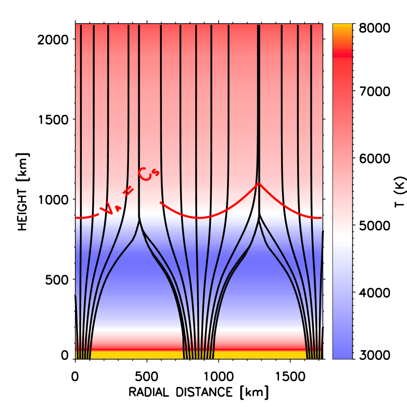
Figure 3: Magnetostatic flux tube model. The background image quantifies the temperature values. The magnetic field along the flux tube axis varies with height from 740 G in the photosphere to 37 G at z=2000 km, the plasma $\beta$ decreases from 4 to 7$\times 10^{-4}$ and the cut-off period increases from 230 s in the photosphere to 280 s in the chromosphere.

4 MHD simulations

To generalize these conclusions (based on a simple model of linear wave propagation) to the case of a more realistic atmosphere with horizontal and vertical stratification in all the physical parameters, a complex magnetic field configuration and non-linear wave propagation, we solved numerically the set of MHD equations in this realistic environment. The numerical code used for the solution of these equations is described elsewhere (Khomenko & Collados, 2006, 2007). Radiative losses were taken into account by means of Newton’s law of cooling. The initial magnetostatic flux tube model was constructed following the method described by Pneuman et al. (1986) (see Fig. 3).

Previous investigations showed that the photospheric driver that excites oscillations inside the flux tube should have a vertical component in order to generate an acoustic fast wave already in the photosphere (Khomenko & Collados, 2007). If this were not the case, no correlation would be observed between the photospheric and chromospheric velocity signals, contrarily to what is suggested by observations (see the power spectra of Fig. 1).

Thus, we applied a vertical periodic driver at the bottom boundary of the simulation domain by varying the vertical velocity as: $V_{z}(x,\it{t})=V_{0}\sin(\omega\it{t})\times\exp(-(x-x_{0})^{2}/2\sigma^{2})$, where $\sigma=160$ km is the horizontal size of the pulse, $V_{0}=200$ m s^-1 is the initial amplitude at the photosphere and $x_{0}$ corresponds to the position of the tube axis. The period of the driver was 300 s (i.e., it is above the cut off period). In what follows we will compare two simulation runs that are identical except for the value of the radiative relaxation time. While the first run is in the adiabatic regime ($\tau_{RR}\rightarrow\infty$), the second one was carried out with $\tau_{RR}=10$ s (constant through the whole atmosphere).

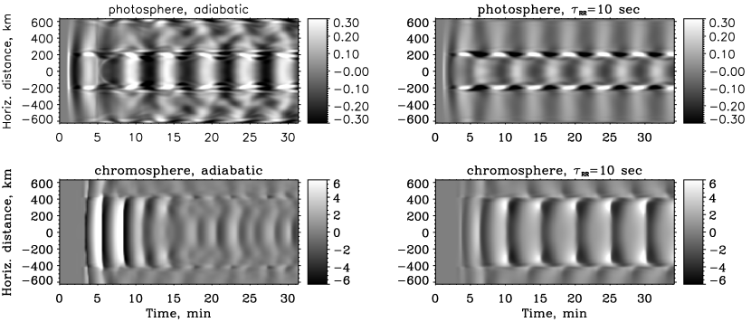
Figure 4: Time-distance plots of the vertical velocity from the simulations at photospheric (top) and chromospheric (bottom) heights. Left: adiabatic calculation; right: calculation with a radiative relaxation time $\tau_{RR}=10$ s. Note how the horizontal extent of the tube is larger in the chromosphere because of the field expansion. The vertical bars on the right of each plot represent the velocity scale in km s^-1.

Figure 5: Left: photospheric (dashed line) and chromospheric (solid line) power spectra obtained from the simulation with $\tau_{RR}$ equal to 10 s. Right: phase difference spectrum for the vertical velocity oscillations. Each cross on the figure is computed as the difference from the chromospheric phase and the photospheric phase for one frequency and one position inside the flux tube.

Fig. 4 gives time-distance plots of the vertical velocity obtained from the simulations at two heights: the upper photosphere around 400 km (top) and the chromosphere around 1500 km (bottom). The vertical photospheric driver generates a fast magneto-acoustic wave that is essentially acoustic in the photosphere where $\beta>1$. This wave propagates upwards through the $\beta=1$ transition layer, preserving its acoustic nature and being transformed into a slow magneto-acoustic mode higher up.

In the adiabatic case (left panels of Fig. 4), we can see that the velocity in the photosphere has a well defined 5-minute periodicity within the flux tube (horizontal distance from -200 to 200 km). Higher up in the chromosphere, this behavior changes. Note that it takes some time for the oscillations to reach the chromospheric heights (bottom panels of Fig. 4). In the chromosphere the tube expands and occupies now a larger area in the time-distance plot (from about -400 to 400 km). At the beginning of the time series, two strong shock waves develop, and are followed in time by strongly damped oscillations. Only weak shocks exist in the stationary phase of the simulations and the wave periodicity is 3 minutes. Thus, in the adiabatic case, there is a shift with height of the dominant period from five minutes in the photosphere to three minutes in the chromosphere.

This behavior contrasts with that of the simulations with $\tau_{RR}=10$ s (right panels of Fig. 4). Contrarily to what happens in the adiabatic case, the 5-minute periodicity is preserved both in the photosphere and in the chromosphere. Waves are linear in the deeper layers, they propagate vertically upwards through the temperature minimum and form shocks with 5-6 km s^-1 amplitudes in the higher layers.

The left panel of Fig. 5 shows the power spectra of the photospheric and chromospheric vertical velocity oscillations in the simulation run with $\tau_{RR}=10$ s. Now there is no shift in the wave period as we go to the higher atmospheric layers, and both the photospheric and chromospheric power spectra are rather similar (right panel). This figure can be directly compared to the observed power spectra in Fig. 1 (left panel). The similarity between the observed and the simulated power spectra is notable. The right panel of Fig. 5 gives the difference in phase between the chromospheric and the photospheric velocity oscillations as a function of frequency, as calculated from the simulations. This figure can be compared with the observed phase spectra in Fig. 1 (right panel). It can be seen that the simulations describe correctly the phase speed of waves in the frequency range 0–5 mHz, as well as the value of the effective cut-off frequency. This gives additional support to our conclusions. Radiative losses are expected to play an important role in small-scale magnetic structures, such as those present in facular regions and, as already shown, they are able to decrease the cut-off frequency allowing the five-minute oscillation to propagate into the chromosphere.

The results shown above were obtained with a fixed value of the radiative relaxation time ($\tau_{RR}=10$ s). We have checked that similar conclusions are reached with a height-dependent relaxation time changing from 10 s in the photosphere to 100 s in the chromosphere.

5 Conclusions

In this paper we have performed an observational, analytical and numerical analysis of the propagation of the 5-min oscillations from the photosphere to the chromosphere in small-scale vertical magnetic flux tubes. From the observational point of view, it has been demonstrated that the power spectra of oscillations in the photosphere and the chromosphere in a facular region are similar and peak at 3 mHz. The observed velocity variations are compatible with the longitudinal acoustic wave propagation in a vertical magnetic field from the photosphere to the chromosphere. The analytical theory of acoustic waves in a stratified isothermal atmosphere embedded in a vertical magnetic field suggests that the effective cut-off frequency can be significantly reduced if the radiative losses of the oscillations are taken into account. This allows the propagation of the evanescent waves at 3 mHz.

The numerical solution of the complete set of the MHD equations allows to generalize this conclusion to the situation of a complex magnetic field configuration, stratification in all atmospheric parameters and non-linear wave effects. We conclude that our photospheric and chromospheric observations can be explained assuming that the radiative relaxation time is sufficiently small (as expected in small-scale magnetic structures). This significantly reduces the cut-off frequency and makes evanescent 5-minute waves propagate vertically from the photosphere towards the chromosphere without changing their period with height. Our conclusion that vertical magnetic field concentrations can also channel the 5-min oscillatory power of the photosphere towards the chromosphere in facular regions extends the actual possibilities of the dynamic and magnetic couplings between these two important layers of the solar atmosphere. Additional work on three-dimensional MHD simulations with non-LTE radiative transfer physics will be necessary to investigate the role of this mechanism in more realistic models of the highly dynamic conditions of the magnetized solar atmosphere.

References

- Avrett et al. (1994) Avrett, E. H., Fontenla, J. M., & Loeser, R. 1994, in Infrared Solar Physics, IAU Symp. No. 154, ed. D. Rabin, J. Jefferies, & C. Lindsey, Vol. 154, 35—47
- Bogdan & Judge (2006) Bogdan, T. J. & Judge, P. G. 2006, in MHD wave and oscillations in the Solar Plasma, Vol. 364, Issue 1839 (Phil. Trans. Royal. Soc.), 313—331
- Centeno et al. (2006a) Centeno, R., Collados, M., & Trujillo Bueno, J. 2006a, in Solar Polarization 4, ed. R. Casini & B. W. Lites, Vol. 358, ASP Conference Series, 465
- Centeno et al. (2006b) Centeno, R., Collados, M., & Trujillo Bueno, J. 2006b, ApJ, 640, 1153
- Centeno et al. (2008a) —. 2008a, ApJ, in preparation
- Centeno et al. (2008b) Centeno, R., Trujillo Bueno, J., Uitenbroek, H., & Collados, M. 2008b, ApJ, submitted
- De Moortel et al. (2002) De Moortel, I., Ireland, J., Hood, A. W., & Walsh, R. W. 2002, A&A, 387, L13
- De Pontieu et al. (2003) De Pontieu, B., Erdelyi, R., & de Wijn, A. G. 2003, ApJ, 595, L63
- De Pontieu et al. (2004) De Pontieu, B., Erdelyi, R. J., & Stewart, P. 2004, Nat, 430, Issue 6999, 536
- Ferraro & Plumpton (1958) Ferraro, V. C. A. & Plumpton, C. 1958, ApJ, 127, 459
- Fleck & Schmitz (1991) Fleck, B. & Schmitz, F. 1991, A&A, 250, 235
- Fleck & Schmitz (1993) —. 1993, A&A, 273, 671
- Jefferies et al. (2006) Jefferies, S. M., McIntosh, S. W., Armstrong, J. D., Bogdan, T., Thomas, J., Cacciani, A., & Fleck, B. 2006, ApJ, 648, L151
- Khomenko & Collados (2006) Khomenko, E. & Collados, M. 2006, ApJ, 653, 739
- Khomenko & Collados (2007) —. 2007, Solar Phys., submitted
- Kneer & Trujillo-Bueno (1987) Kneer, F. & Trujillo Bueno, J. 1987, A&A, 183, 91
- Krijger et al. (2001) Krijger, J. M., Rutten, R. J., Lites, B. W., Straus, T., Shine, R. A., & Tarbell, T. D. 2001, A&A, 379, 1052
- Martínez Pillet et al. (1999) Martínez Pillet, V., Collados, M., Sánchez Almeida, J., González, V., Cruz-Lopez, A., Manescau, A., Joven, E., Paez, E., Diaz, J., Feeney, O., Sánchez, V., Scharmer, G., & Soltau, D. 1999, in High resolution solar physics: theory, observations and techniques, ed. T. R. Rimmele, K. S. Balasubramaniam, & R. R. Radick, Vol. 183, 19th NSO/SP Summer Workshop (ASP Conf. Series), 264
- Mihalas & Mihalas (1984) Mihalas, D. & Mihalas, B. W. 1984, Foundations of Radiation Hydrodynamics (Oxford: Oxford University Press)
- Pneuman et al. (1986) Pneuman, G. W., Solanki, S. K., & Stenflo, J. O. 1986, A&A, 154, 231
- Pozhalova (1988) Pozhalova, Z. A. 1988, Soviet Astr., 32, N 5, 542
- Roberts (1983) Roberts, B. 1986, Solar Phys., 87, 77
- Roberts (2006) Roberts, B. 2006, Royal Society of London Transactions Series A, 364, Issue 1839, 447
- Spiegel (1957) Spiegel, E. A. 1957, ApJ, 126, 202
- Vecchio et al. (2007) Vecchio, A., Cauzzi, G., Reardon, K. P., Janssen, K., & Rimmele, T. 2007, A&A, 461, L1