Non-Hermitian spectral effects in a $\mathcal{PT}$-symmetric waveguide

Abstract

We present a numerical study of the spectrum of the Laplacian in an unbounded strip with $\mathcal{PT}$-symmetric boundary conditions. We focus on non-Hermitian features of the model reflected in an unusual dependence of the eigenvalues below the continuous spectrum on various boundary-coupling parameters.

1 Introduction

In the last years the theory of quasi-Hermitian, pseudo-Hermitian and $\mathcal{PT}$-symmetric operators has developed rapidly, and has been shown to provide a huge class of non-Hermitian Hamiltonians with real spectra (cf the pioneering works [24, 4, 23] and the review [3] with many references). Because of these recent observations, the condition of self-adjointness of operators representing observables in quantum mechanics may seem to be rather an annoying technicality. However, unless it is met one cannot apply the very powerful machinery of spectral theory based on the spectral theorem.

In particular, one has to restrict to exactly solvable models [22, 27, 25, 18, 21] or to rely on perturbation and numerical methods to analyse the spectrum of the $\mathcal{PT}$-symmetric Hamiltonians. Except for some simple one-dimensional examples [2], the majority of the $\mathcal{PT}$-symmetric models studied in the literature have purely discrete spectrum. Perturbation methods are then notably effective in determining the dependence of the eigenvalues on various parameters of the given model. Although the perturbation approach can even prove that the total spectrum is real in some cases [20, 8, 7, 9], it is limited in its nature and one usually has to employ numerical techniques in order to obtain a more complete picture of the spectral properties.

In a way motivated by the lack of a well-developed spectral theory for non-self-adjoint operators with non-compact resolvent, in a recent paper [6] Borisov and one of the present authors introduced a new two-dimensional $\mathcal{PT}$-symmetric Hamiltonian with a real continuous spectrum. One of the main questions arising within this model is whether the Hamiltonian possesses point spectrum, too. Using some singular perturbation techniques adopted from the theory of quantum waveguides [13, 5], the question was given both positive and negative answer in [6], depending on the nature of the effective $\mathcal{PT}$-symmetric interaction in a weakly-coupled regime. Moreover, in the case when the point spectrum exists, the weakly-coupled eigenvalues emerging from the continuous spectrum were shown to be real. We refer to the next Section 2 for a precise statement of the spectral results established in [6].

In the present paper, we further analyse the question of the existence of point spectrum for the Hamiltonian introduced in [6] by numerical methods. This enables us to explore quantitative properties of the eigenvalues without the restriction to the weakly-coupled regime. The main emphasis is put on peculiar characteristics of the model which are related to the non-self-adjointness of the underlying Hamiltonian, namely:

1. highly non-monotone dependence of the eigenvalues on a coupling parameter; as the parameter increases, the eigenvalues emerge from the continuous spectrum, reach a minimum, sometimes disappear in the continuous spectrum, emerge later on again, etc;

2. broken $\mathcal{PT}$-symmetry; as the coupling parameter increases, the eigenvalues may emerge from the continuous spectrum as complex-conjugate pairs, collide and become real, move on the real axis, collide again and become complex, etc.

This paper is organized as follows. We begin by recalling the Hamiltonian from [6] and summarize the main spectral properties established there. In particular, we point out some questions the study of [6] has left open. In Section 3 we describe the numerical methods we use. The numerical data are then presented and discussed in Section 4. In the final Section 5 we make some conjectures based on the present study.

2 The model, known results and open questions

Given a positive number $d$, we introduce an infinite strip $\Omega:=\mathbb{R}\times(0,d)$. We split the variables consistently by writing $x=(x_{1},x_{2})$ with $x_{1}\in\mathbb{R}$ and $x_{2}\in(0,d)$. Let $\alpha:\mathbb{R}\to\mathbb{R}$ be a bounded function; occasionally we shall denote by the same symbol the function $x\mapsto\alpha(x_{1})$ on $\Omega$. The Hamiltonian $H_{\alpha}$ we consider in this paper acts simply as the Laplacian in the Hilbert space $L^{2}(\Omega)$, i.e.

$$H_{\alpha}\Psi:=-\Delta\Psi\qquad\mbox{in}\quad\Omega\,,$$ (1)

and a non-trivial interaction is introduced by choosing as its domain the set of functions $\Psi$ from $\mathop{W^{2,2}}\nolimits(\Omega)$ satisfying the following Robin-type boundary conditions:

$$\partial_{2}\Psi+\mathrm{i}\,\alpha\,\Psi\,=\,0\qquad\mbox{on}\quad\partial\Omega\,.$$ (2)

Here $\mathop{W^{2,2}}\nolimits(\Omega)$ denotes the Sobolev space consisting of functions on $\Omega$ which, together with all their first and second distributional derivatives, are square integrable. As usual, the action of $H_{\alpha}$ should be understood in the distributional sense and (2) should be understood in the sense of traces [1].

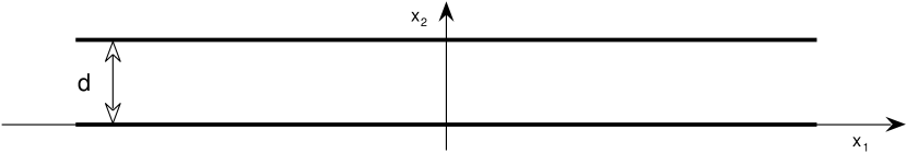
Figure 1: A schematic view of an infinite planar waveguide of width $d$. The Robin conditions (2) are imposed at the boundary.

Under the additional hypothesis that $\alpha$ possesses a bounded distributional derivative, i.e. $\alpha\in W^{1,\infty}(\mathbb{R})$, it was shown in [6] that $H_{\alpha}$ is an $m$-sectorial operator satisfying

$$H_{\alpha}^{*}=H_{-\alpha}\,,$$ (3)

where $H_{\alpha}^{*}$ denotes the adjoint of $H_{\alpha}$. (If $\alpha$ is merely bounded, it is still possible to give a meaning to $H_{\alpha}$ by using the quadratic-form approach.) Of course, $H_{\alpha}$ is not self-adjoint unless $\alpha$ vanishes identically. However, the relation (3) reflects the $\mathcal{PT}$-symmetry – or, more generally and more precisely, the $\mathcal{T}$-self-adjointness – of $H_{\alpha}$, with $\mathcal{P}$ and $\mathcal{T}$ being defined by $(\mathcal{P}\Psi)(x):=\Psi(d-x)$ and $\mathcal{T}\Psi:=\overline{\Psi}$, respectively.

An important property of the operator $H_{\alpha}$ being $m$-sectorial is that it is closed. Then, in particular, the spectrum $\sigma(H_{\alpha})$ is well defined as the set of complex points $z$ such that $H_{\alpha}-z$ is not bijective. The point spectrum $\sigma_{\mathrm{p}}(H_{\alpha})$ equals the set of points $z$ such that $H_{\alpha}-z$ is not injective. The continuous spectrum $\sigma_{\mathrm{c}}(H_{\alpha})$ equals the set of points $z$ such that $H_{\alpha}-z$ is not surjective but the range of $H_{\alpha}-z$ is dense in $L^{2}(\Omega)$. Finally, the residual spectrum $\sigma_{\mathrm{r}}(H_{\alpha})$ equals the set of points $z$ such that $H_{\alpha}-z$ is injective but the range of $H_{\alpha}-z$ is not dense in $L^{2}(\Omega)$.

In the following theorem we collect general results about the spectrum of $H_{\alpha}$ established in [6]:

Theorem 1.

Let $\alpha\in W^{1,\infty}(\mathbb{R})$ and $\alpha_{0}\in\mathbb{R}$. Then

• $\sigma(H_{\alpha})\subseteq\{z\in\mathbb{C}\,:\,|\arg(z)|\leq\theta\}$ with some $\theta\in[0,\pi/2)$;

• $\sigma_{\mathrm{r}}(H_{\alpha})=\varnothing$;

• $\sigma(H_{\alpha_{0}})=\sigma_{\mathrm{c}}(H_{\alpha_{0}})=[\mu_{0}^{2},\infty)$  where  $\mu_{0}:=\min\{|\alpha_{0}|,\pi/d\}$;

• if $\alpha-\alpha_{0}\in C_{0}(\mathbb{R})$, then  $\sigma_{\mathrm{c}}(H_{\alpha})=[\mu_{0}^{2},\infty)$;

• if $\alpha\in C_{0}(\mathbb{R})$ is an odd function, then  $\sigma_{\mathrm{p}}(H_{\alpha})\subset\mathbb{R}$;

Here $C_{0}(\mathbb{R})$ denotes the space of continuous functions on $\mathbb{R}$ with compact support. Note that $\alpha\in C_{0}(\mathbb{R})\cap W^{1,\infty}(\mathbb{R})$ implies that $\alpha$ is Lipschitz continuous; conversely, the space of Lipschitz continuous functions on $\mathbb{R}$ is embedded in $W^{1,\infty}(\mathbb{R})$.

The first two properties of Theorem 1 are quite general: (i) holds since $H_{\alpha}$ is sectorial and (ii) is a consequence of the $\mathcal{T}$-self-adjointness (we refer to [6] for more details). Since the spectral problem for the constant case of (iii) can be solved by some sort of “separation of variables” (cf [6, Sec. 4]), we shall refer to it as the unperturbed case; it follows from Theorem 1 that the corresponding spectrum is purely continuous and positive. As a consequence of (ii), (iv) and (v), we get a result about the reality of the total spectrum in the perturbed case:

Corollary 1.

Let $\alpha\in C_{0}(\mathbb{R})\cap W^{1,\infty}(\mathbb{R})$ be an odd function. Then

$$\sigma(H_{\alpha})\subset\mathbb{R}\,.$$

The result stated in part (iv) of Theorem 1 makes rigorous the heuristic statement that “the continuous spectrum depends on the properties of a Hamiltonian interaction at infinity only”. On the other hand, it is well known – and this already for one-dimensional self-adjoint models [17] – that the point spectrum may be highly unstable under a perturbation of an operator with non-compact resolvent. In [6], the point spectrum of $H_{\alpha}$ was analysed perturbatively in the weakly-coupled regime:

$$\alpha=\alpha_{0}+\varepsilon\,\beta\,,\qquad\mbox{with}\quad\alpha_{0}\in\mathbb{R}\,,\ \varepsilon>0\,,\ \beta\in C_{0}^{2}(\mathbb{R})\,,\$$ (4)

where $\beta$ is assumed to be real-valued and $\varepsilon$ plays the role of the small parameter. Here $C_{0}^{2}(\mathbb{R})$ denotes the space of functions on $\mathbb{R}$ which, together with all their first and second derivatives, are continuous and have compact support. The main interest was focused on the existence and asymptotic behavior of the eigenvalues emerging from the threshold $\mu_{0}^{2}$ of the continuous spectrum due to the perturbation of $H_{\alpha_{0}}$ by $\varepsilon\beta$.

Before stating the main results of [6] about the weakly-coupled eigenvalues, we need to introduce some notation. Recalling the definition of $\mu_{0}$ from Theorem 1.(iii), we next define

$$\mu_{1}:=\max\{|\alpha_{0}|,\pi/d\}\qquad\mbox{and}\qquad\mu_{j}:=\pi j/d\quad\mbox{for}\quad j\geq 2\,.$$

To these numbers we associate a family of functions $\{\psi_{j}\}_{j=0}^{\infty}$ by

$$\psi_{j}(x_{2}):=\cos(\mu_{j}x_{2})-\mathrm{i}\,\frac{\alpha_{0}}{\mu_{j}}\,\sin(\mu_{j}x_{2})\,.$$ (5)

Let $\{v_{j}\}_{j=0}^{\infty}$ be a sequence of auxiliary functions given by

$$v_{j}(x_{1}):=\left\{\begin{aligned} &-\frac{1}{2}\int_{\mathbb{R}}|x_{1}-t_{1}|\beta(t_{1})\,dt_{1}&\text{if}\quad j=0\,,\\ &\frac{1}{2\sqrt{\mu_{j}^{2}-\mu_{0}^{2}}}\int_{\mathbb{R}}e^{-\sqrt{\mu_{j}^{2}-\mu_{0}^{2}}|x_{1}-t_{1}|}\beta(t_{1})\,dt_{1}&\text{if}\quad j\geq 1\,.\end{aligned}\right.$$

Finally, denoting $\langle f\rangle=\int_{\mathbb{R}}f(x_{1})\,dx_{1}$ for any $f\in L^{1}(\mathbb{R})$, we introduce a constant $\tau$, depending on $\beta$, $d$ and $\alpha_{0}$, by

$$\tau:=\left\{\begin{aligned} &2\alpha_{0}^{2}\langle\beta v_{0}\rangle+\frac{2\alpha_{0}}{d}\sum\limits_{j=1}^{\infty}\frac{\mu_{j}^{2}\langle\beta v_{j}\rangle}{\mu_{j}^{2}-\mu_{0}^{2}}\,\tan\frac{\alpha_{0}d+j\pi}{2}\ &\text{if}\quad|\alpha_{0}|<\frac{\pi}{d}\,,\\ &\frac{2\alpha_{0}\pi^{2}\cot\frac{\alpha_{0}d}{2}}{(\mu_{1}^{2}-\mu_{0}^{2})d^{3}}\langle\beta v_{1}\rangle+\frac{8\pi^{2}}{(\mu_{1}^{2}-\mu_{0}^{2})d^{4}}\sum\limits_{j=1}^{\infty}\frac{\mu_{2j}^{2}\langle\beta v_{2j}\rangle}{\mu_{2j}^{2}-\mu_{1}^{2}}\ &\text{if}\quad|\alpha_{0}|>\frac{\pi}{d}\,.\end{aligned}\right.$$ (6)

Now we are in a position to take over from [6]:

Theorem 2.

Let $\alpha$ be given by (4).

• If $\alpha_{0}=0$, then $H_{\alpha}$ has no eigenvalues converging to $\mu_{0}^{2}$ as $\varepsilon\to 0$.

• Let $0<|\alpha_{0}|<\pi/d$.

  1. If $\alpha_{0}\langle\beta\rangle<0$, then there exists the unique eigenvalue $\lambda_{\varepsilon}$ of $H_{\alpha}$ converging to $\mu_{0}^{2}$ as $\varepsilon\to 0$. This eigenvalue is simple and real, and satisfies the asymptotic formula

     $$\lambda_{\varepsilon}=\mu_{0}^{2}-\varepsilon^{2}\alpha_{0}^{2}\langle\beta\rangle^{2}+2\varepsilon^{3}\alpha_{0}\tau\langle\beta\rangle+\mathcal{O}(\varepsilon^{4})\,.$$ (7)

  2. If $\alpha_{0}\langle\beta\rangle>0$, then $H_{\alpha}$ has no eigenvalues converging to $\mu_{0}^{2}$ as $\varepsilon\to 0$.

  3. If $\langle\beta\rangle=0$ and $\tau>0$, then there exists the unique eigenvalue $\lambda_{\varepsilon}$ of $H_{\alpha}$ converging to $\mu_{0}^{2}$ as $\varepsilon\to 0$. This eigenvalue is simple and real, and satisfies the asymptotics

     $$\lambda_{\varepsilon}=\mu_{0}^{2}-\varepsilon^{4}\tau^{2}+\mathcal{O}(\varepsilon^{5})\,.$$ (8)

  4. If $\langle\beta\rangle=0$ and $\tau<0$, then $H_{\alpha}$ has no eigenvalues converging to $\mu_{0}^{2}$ as $\varepsilon\to 0$.

• Let $|\alpha_{0}|>\pi/d$  and  $\alpha_{0}d/\pi\not\in\mathbb{Z}$.

  1. If $\tau>0$, then there exists the unique eigenvalue $\lambda_{\varepsilon}$ of $H_{\alpha}$ converging to $\mu_{0}^{2}$ as $\varepsilon\to 0$, it is simple and real, and satisfies the asymptotics (8).

  2. If $\tau<0$, then $H_{\alpha}$ has no eigenvalues converging to $\mu_{0}^{2}$ as $\varepsilon\to 0$.

The method of [6] gives also the asymptotic expansion of the eigenfunctions corresponding to the weakly-coupled eigenvalues:

Theorem 3.

The eigenfunction $\Psi_{\varepsilon}$ corresponding to any eigenvalue $\lambda_{\varepsilon}$ from Theorem 2 can be chosen so that it satisfies the asymptotics

$$\Psi_{\varepsilon}(x)=\psi_{0}(x_{2})+\mathcal{O}(\varepsilon)$$ (9)

in $\mathop{W^{2,2}}\nolimits(\Omega\cap\{x:|x_{1}|<a\})$ for each $a>0$, and behaves at infinity as

$$\Psi_{\varepsilon}(x)=\exp^{-\sqrt{\mu_{0}^{2}-\lambda_{\varepsilon}}|x_{1}|}\psi_{0}(x_{2})+\mathcal{O}(\exp^{-\sqrt{\mu_{0}^{2}-\lambda_{\varepsilon}}|x_{1}|})\,,\quad x_{1}\to+\infty\,.$$ (10)

Theorems 1–3 summarizing the spectral analysis performed in [6] leave open the following particular questions:

1. Can the cases (B4) and (C2) of Theorem 2 occur? That is, can the constant $\tau$ be negative for a certain combination of $d,\alpha_{0}$ and $\beta$? (Sufficient conditions for the positivity of $\tau$ exist [6, Props. 2.1–2.2].)

2. What happens in the case (C) of Theorem 2 if the condition $\alpha_{0}d/\pi\not\in\mathbb{Z}$ is not satisfied? Is it just a technical hypothesis?

3. Is there any point spectrum in the case of Corollary 1?

4. What is the dependence of the weakly-coupled eigenvalues of Theorem 2 as the parameter $\varepsilon$ increases?

5. Do the eigenvalues remain real for large $\varepsilon$?

6. Can one have more eigenvalues? Can they be degenerate? What is the dependence of the number of eigenvalues on $\varepsilon$?

7. Are there any eigenvalues emerging from other thresholds $\mu_{j}^{2}$, $j\geq 1$? Can they emerge from other points of the continuous spectrum, different from the thresholds $\mu_{j}^{2}$, $j\geq 0$?

The main goal of the present paper is to provide answers to some of these questions by a numerical study of the spectral problem.

3 Numerical methods

In order to get the dependence of the bound states on parameters like $\varepsilon,d,\alpha_{0}$, etc, numerically we used two independent methods. When $\alpha$ is a simple step-like function (e.g. symmetric or asymmetric square well), we treat the problem by mode matching method. It takes into account the asymptotic behaviour of solution explicitly and can serve thus as a useful check when we apply the other method, viz, the spectral method. This method is more robust and we use it for more general $\alpha$. We arrived at an excellent agreement in cases when both methods are applicable.

3.1 Mode matching method

Let us begin with mode matching. The most general situation we want to describe is shown in Figure 2. Fix negative and positive numbers $L_{-}$ and $L_{+}$, respectively. In the asymptotic regions, i.e. $x_{1}<L_{-}$ and $L_{+}<x_{1}$, we assume $\alpha(x_{1})=\alpha_{0}$, while in the central parts we have $\alpha(x_{1})=\alpha_{-}$ if $L_{-}<x_{1}<0$ and $\alpha(x_{1})=\alpha_{+}$ if $0<x_{1}<L_{+}$.

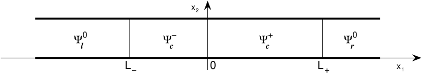
Figure 2: The mode matching approach. A particular Ansatz (11) for an eigenfunction $\Psi$ of $H_{\alpha}$ corresponding to $\lambda$ is chosen in each subregion and the smooth matching (3.1) is required at the boundaries separating the subregions.

Let $\{\mu_{j}^{\pm}\}_{j=0}^{\infty}$ denote the sequence of numbers $\{\mu_{j}\}_{j=0}^{\infty}$ with $\alpha_{0}$ being replaced by $\alpha_{\pm}$. In the same way we define the sequence of functions $\{\psi_{j}^{\pm}\}_{j=0}^{\infty}$ by replacing $\alpha_{0}$ by $\alpha_{\pm}$ in (5). In order to make the notation more consistent, hereafter we write $\mu_{j}^{0}$ and $\psi_{j}^{0}$ instead of $\mu_{j}$ and $\psi_{j}$, respectively, and introduce a common index $\iota\in\{0,+,-\}$.

In each of the regions where $\alpha$ is constant, the spectral problem $-\Delta\Psi=\lambda\Psi$, with $\Psi$ satisfying the required boundary conditions, can be solved explicitly [6, Sec. 4] by expanding $\Psi$ into the “transverse basis” $\{\psi_{j}^{\iota}\}_{j=0}^{\infty}$, where $\iota$ depends on the region. More specifically, we use the following Ansatz for an eigenfunction $\Psi$ of $H_{\alpha}$ corresponding to $\lambda$:

$$\Psi(x)=\left\{\begin{aligned} \Psi_{l}^{0}(x)&:=\sum_{j=0}^{\infty}d_{j}\,e^{\sqrt{(\mu_{j}^{0})^{2}-\lambda}\,x_{1}}\,\psi_{j}^{0}(x_{2})&\mbox{if}&\quad x_{1}\in(-\infty,L_{-})\,,\\ \Psi_{c}^{-}(x)&:=\sum_{j=0}^{\infty}c_{j}\,\varphi_{j}^{-}(x_{1})\,\psi_{j}^{-}(x_{2})&\mbox{if}&\quad x_{1}\in(L_{-},0)\,,\\ \Psi_{c}^{+}(x)&:=\sum_{j=0}^{\infty}b_{j}\,\varphi_{j}^{+}(x_{1})\,\psi_{j}^{+}(x_{2})&\mbox{if}&\quad x_{1}\in(0,L_{+})\,,\\ \Psi_{r}^{0}(x)&:=\sum_{j=0}^{\infty}a_{j}\,e^{-{\sqrt{(\mu_{j}^{0})^{2}-\lambda}\,x_{1}}}\,\psi_{j}^{0}(x_{2})&\mbox{if}&\quad x_{1}\in(L_{+},+\infty)\,,\\ \end{aligned}\right.$$ (11)

where

$$\varphi_{j}^{\pm}(x_{1}):=\cos\big{(}\sqrt{\lambda-(\mu_{j}^{\pm})^{2}}\,x_{1}\big{)}+B_{\pm}\,\sin\big{(}\sqrt{\lambda-(\mu_{j}^{\pm})^{2}}\,x_{1}\big{)}\,.$$

Standard elliptic regularity theory implies that any weak solution $\Psi$ to $-\Delta\Psi=\lambda\Psi$ is necessarily infinitely smooth in the interior of $\Omega$. In particular, we must match the functions from the Ansatz smoothly at $x_{1}=L_{-},0,L_{+}$, i.e. we require

$$\Psi_{l}^{0}(L_{-},x_{2}) =\Psi_{c}^{-}(L_{-},x_{2})\,, \partial_{1}\Psi_{l}^{0}(L_{-},x_{2}) =\partial_{1}\Psi_{c}^{-}(L_{-},x_{2})\,,$$

$$\Psi_{c}^{-}(0,x_{2}) =\Psi_{c}^{+}(0,x_{2})\,, \partial_{1}\Psi_{c}^{-}(0,x_{2}) =\partial_{1}\Psi_{c}^{+}(0,x_{2})\,,$$ (12)

$$\Psi_{c}^{+}(L_{+},x_{2}) =\Psi_{r}^{0}(L_{+},x_{2})\,, \partial_{1}\Psi_{c}^{+}(L_{+},x_{2}) =\partial_{1}\Psi_{+}^{0}(L_{+},x_{2})\,,$$

for every $x_{2}\in(0,d)$.

If $\{\psi_{j}^{\iota}\}_{j=0}^{\infty}$ formed an orthonormal family, the next step would consist in employing the orthonormality and reducing (3.1) into a system of algebraic equations for the coefficients $a_{j},b_{j},c_{j},d_{j}$. However, since the family $\{\psi_{j}^{\iota}\}_{j=0}^{\infty}$ is actually formed by eigenfunctions of a transverse eigenvalue problem which is not Hermitian (unless $\alpha_{\iota}=0$), it is clear that the functions $\psi_{j}^{\iota}$ are not mutually orthogonal in general. Instead, we use the property that $\{\psi_{j}^{\iota}\}_{j=0}^{\infty}$ and $\{\phi_{j}^{\iota}\}_{j=0}^{\infty}$ form a complete biorthonormal pair [18], where $\phi_{j}^{\iota}$ are properly normalized eigenfunctions of the adjoint transverse problem:

$$\phi_{j}^{\iota}(x_{2}):=\overline{A_{j}^{\iota}\,\psi_{j}^{\iota}(x_{2})}\,.$$

The normalization constants can be chosen as follows

$$A_{j_{0}}^{\iota}:=\frac{2\mathrm{i}\alpha_{\iota}}{1-\exp{(-2\mathrm{i}\alpha_{\iota}d)}}\,,\quad A_{j_{1}}^{\iota}:=\frac{2(\mu_{1}^{\iota})^{2}}{[(\mu_{1}^{\iota})^{2}-\alpha_{\iota}^{2}]d}\,,\quad A_{j}^{\iota}:=\frac{2(\mu_{j}^{\iota})^{2}}{[(\mu_{j}^{\iota})^{2}-\alpha_{\iota}^{2}]d}\,,$$

where $j\geqslant 2$, $(j_{0},j_{1})=(0,1)$ if $|\alpha_{\iota}|<\pi/d$ and $(j_{0},j_{1})=(1,0)$ if $|\alpha_{\iota}|>\pi/d$ (if $\alpha_{\iota}=0$, the fraction in the definition of $A_{j_{0}}^{\iota}$ should be understood as the expression obtained after taking the limit $\alpha_{\iota}\to 0$). Then, in particular, we have

$$\forall i,j\in\mathbb{N},\quad(\phi_{i}^{\iota},\psi_{j}^{\iota})=\delta_{ij}\,,$$ (13)

where $(\cdot,\cdot)$ denotes the inner product in $L^{2}((0,d))$, antilinear in the first factor and linear in the second one.

Now, multiplying (3.1) by $\overline{\phi_{i}^{0}}$, integrating over $x_{2}\in(0,d)$ and employing (13) in the asymptotic regions, we can eliminate the coefficients $a_{j}$ and $d_{j}$ by means of the relations

$$a_{i}\,e^{-\sqrt{(\mu_{i}^{0})^{2}-\lambda}\,L_{+}} =\sum_{j=0}^{\infty}b_{j}\,\varphi_{j}^{+}(L_{+})\,(\phi_{i}^{0},\psi_{j}^{+})\,,$$ (14)

$$d_{i}\,e^{\sqrt{(\mu_{i}^{0})^{2}-\lambda}\,L_{-}} =\sum_{j=0}^{\infty}c_{j}\,\varphi_{j}^{-}(L_{-})\,(\phi_{i}^{0},\psi_{j}^{-})\,,$$

for every $i\in\mathbb{N}$, and reduce thus the number of conditions to be fulfilled. We finally arrive at an infinite-dimensional homogeneous system

$$\left(\begin{array}[]{c c c c}m_{11}&m_{12}&0&0\\ m_{21}&0&m_{23}&0\\ 0&0&m_{33}&m_{34}\\ 0&m_{42}&0&m_{44}\end{array}\right)\left(\begin{array}[]{c}b\\ c\\ bB_{+}\\ cB_{-}\end{array}\right)=\left(\begin{array}[]{c}0\\ 0\\ 0\\ 0\end{array}\right)\,.$$ (15)

Here $b,c$ denote the infinite vectors formed by $b_{j},c_{j}$, respectively, and the submatrices $m_{\mu\nu}$ are given by

$$m_{11} :=(\phi_{i}^{0},\psi_{j}^{+})\,, m_{33} :=\sqrt{\lambda-(\mu_{j}^{+})^{2}}\,(\phi_{i}^{0},\psi_{j}^{+})\,,$$

$$m_{12} :=-(\phi_{i}^{0},\psi_{j}^{-})\,, m_{34} :=-\sqrt{\lambda-(\mu_{j}^{-})^{2}}\,(\phi_{i}^{0},\psi_{j}^{-})\,,$$

$$m_{21} :=\bigg{(}\mbox{$\sqrt{(\mu_{i}^{0})^{2}-\lambda}$}\,\cos\big{(}L_{+}\sqrt{\lambda-(\mu_{j}^{+})^{2}}\big{)}$$

$$\qquad\qquad-\sqrt{\lambda-(\mu_{j}^{+})^{2}}\,\sin\big{(}L_{+}\sqrt{\lambda-(\mu_{j}^{+})^{2}}\big{)}\bigg{)}(\phi_{i}^{0},\psi_{j}^{+})\,,$$

$$m_{23} :=\bigg{(}\sqrt{(\mu_{i}^{0})^{2}-\lambda}\,\sin\big{(}L_{+}\sqrt{\lambda-(\mu_{j}^{+})^{2}}\big{)}$$

$$\qquad\qquad+\sqrt{\lambda-(\mu_{j}^{+})^{2}}\,\cos\big{(}L_{+}\sqrt{\lambda-(\mu_{j}^{+})^{2}}\big{)}\bigg{)}(\phi_{i}^{0},\psi_{j}^{+})\,,$$

$$m_{42} :=\bigg{(}\sqrt{(\mu_{i}^{0})^{2}-\lambda}\,\cos\big{(}L_{-}\sqrt{\lambda-(\mu_{j}^{-})^{2}}\big{)}$$

$$\qquad\qquad+\sqrt{\lambda-(\mu_{j}^{-})^{2}}\,\sin\big{(}L_{-}\sqrt{\lambda-(\mu_{j}^{-})^{2}}\big{)}\bigg{)}(\phi_{i}^{0},\psi_{j}^{-})\,,$$

$$m_{44} :=\bigg{(}\sqrt{(\mu_{i}^{0})^{2}-\lambda}\,\sin\big{(}L_{-}\sqrt{\lambda-(\mu_{j}^{-})^{2}}\big{)}$$

$$\qquad\qquad-\sqrt{\lambda-(\mu_{j}^{-})^{2}}\,\cos\big{(}L_{-}\sqrt{\lambda-(\mu_{j}^{-})^{2}}\big{)}\bigg{)}(\phi_{i}^{0},\psi_{j}^{-})\,,$$

where the right hand sides should be understood as the infinite matrices formed by the respective coefficients for $i,j\in\mathbb{N}$. Our numerical approximation then consists in approximating the infinite system by using finite submatrices for $i,j\in\{0,\dots,N\}$ with $N$ large enough.

In order to have a nontrivial solution we require

$$\det\left(\begin{array}[]{c c c c}m_{11}&m_{12}&0&0\\ m_{21}&0&m_{23}&0\\ 0&0&m_{33}&m_{34}\\ 0&m_{42}&0&m_{44}\end{array}\right)=0\,,$$ (16)

which gives an implicit equation for $\lambda$ as the unknown. Having found $\lambda$, we can then calculate the coefficients $a_{j},b_{j},c_{j},d_{j},B_{\pm,j}$ from (15) and (14).

If $\alpha_{+}=\alpha_{-}$ and $L_{+}=-L_{-}$, i.e. $\alpha$ is a symmetric square well, then (16) can be reduced to

$$\det\left(\begin{array}[]{c c}m_{21}+m_{42}&0\\ 0&m_{23}-m_{44}\end{array}\right)=0\,.$$

The solutions have different symmetry with respect to $x_{1}\mapsto-x_{1}$, the even solutions are formed only of cosines, the odd of sines.

Remark.

In principle, it is possible to extend the present method to an arbitrary piece-wise constant function $\alpha$, provided that the number of matching interfaces is finite. On the other hand, the more matching conditions the bigger size of the matrix of (15) and thus the higher (numerical) price one must pay.

3.2 Spectral method

In order to treat the waveguide with a general $\alpha$ in the boundary conditions, we decided to use spectral collocation methods. They provide a reliable and rapidly converging tool easily applicable to our model. A very useful software suite has already been published [26]. It could be adapted to this problem. We approximate the operator by a series of operators defined on a finite domain $[x_{1}^{min},x_{1}^{max}]\times[0,d]$ with Dirichlet boundary conditions on $\{x_{1}^{min}\}\times[0,d]$ and $\{x_{1}^{max}\}\times[0,d]$.

First, we can form the differentiation matrices in each variable separately and then combine them to the two-dimensional problem. The infinite domain in $x_{1}$-variable suggests that we could approximate it by grid points chosen as the roots of Hermite polynomials and as an interpolant we take Lagrange polynomial. There is an additional parameter (the real line can be mapped to itself by a change of variable $x_{1}=b\tilde{x}_{1},b>0$), which can be used to optimize the choice of the grid points together with variation of the number of roots $N_{1}$. The roots span the interval $[\xi_{1},\xi_{N_{1}}]$, $-\xi_{1}=\xi_{N_{1}}$, cluster around the origin, and grow as $\xi_{N_{1}}=\mathcal{O}(\sqrt{N_{1}})$ for $N_{1}\rightarrow\infty$.

Another possibility is to use Fourier differencing. We form a uniform grid in $[-x_{1}^{max},x_{1}^{max}]$ and since the solutions decay exponentially, we can theoretically extend it periodically across this interval to the whole $\mathbb{R}$. The interpolant is a trigonometric function.

In both approaches the interpolant is an infinitely differentiable function. Deriving it and taking the derivatives in the grid points we get the differentiation matrices. Imposing the homogeneous Dirichlet boundary conditions consists in deleting the first and the last rows and columns of the differentiation matrices.

The transversal variable is confined to a finite interval $[0,d]$ and it is possible to scale it to $[-1,1]$. To implement the boundary conditions we prefer to incorporate them into the interpolant. It requires to use Hermite interpolation, which takes into account derivative values in addition to function values. The use of the roots of Chebyshev polynomials $\eta_{k}=\cos((k-1)\pi/(N_{2}-1)),k=1,\ldots,N_{2}$ as the grid points is common here. For details we refer the reader to [26].

Now, it remains to form differentiation matrices that correspond to partial derivatives entering the Laplacian. Having set up a grid in each direction we combine them into the tensor product grid. Then a closer inspection shows that $\partial_{1}^{2}\rightarrow D^{(2)}(x_{1})\otimes\mathbf{I}$, where $\mathbf{I}$ is an $N_{2}\times N_{2}$ identity matrix and $\partial_{2}^{2}$ is constructed in a similar way (it is necessary to take into account that the boundary conditions change with $x_{1}$).

Applying the spectral discretization we converted the search for eigenvalues of $H_{\alpha}$ to a matrix eigenvalue problem.

4 Discussion of numerical results

Existence of eigenvalues below the threshold of the continuous spectrum and their behaviour for weak perturbations was already proved in [6]. Our calculations confirm it and demonstrate that the spectrum of eigenvalues is considerably richer.

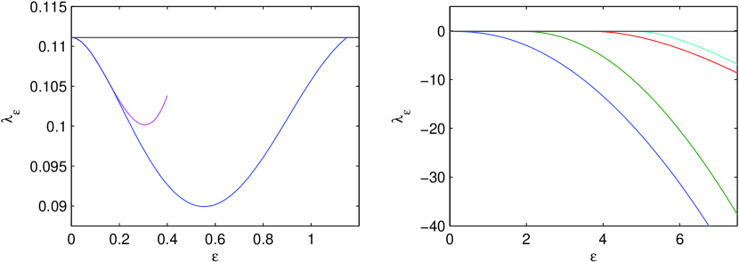
Figure 3: Comparison of dependence of eigenvalues on $\varepsilon$ for $\mathcal{PT}$-symmetric and self-adjoint waveguides. The left figure shows the $\mathcal{PT}$-symmetric case with $\alpha(x_{1})=1/3-\varepsilon\exp(-x_{1}^{2})$. Here the blue (respectively magenta) curve represents the eigenvalue (respectively the asymptotic formula (7) up to the $\varepsilon^{3}$-term). The right figure shows the eigencurves in the corresponding self-adjoint situation, obtained by replacing $\mathrm{i}\alpha\mapsto\alpha$ in (2). $d=2$ in both cases.

A typical dependence of an eigenvalue on the perturbation parameter $\varepsilon$ is shown in Figure 3. Here we perturbed a waveguide of width $d=2$ and $\alpha_{0}=1/3$ by a Gaussian shape, i.e. we took $\beta(x_{1})=-\exp(-x_{1}^{2})$ in (4). Since $0<\alpha_{0}<\pi/d$ and $\langle\beta\rangle<0$, we deal with the case (B1) of Theorem 2. We observe that the asymptotic expansion (7) is fairly good. It is striking, however, that the dependence of the eigenvalue on $\varepsilon$ is highly non-monotonic: The eigenvalue appears at some value of $\varepsilon$ (in this case it is $\varepsilon=0$), reaches a minimum, and then returns to the continuous spectrum. We found such a behaviour in all cases we studied, viz, various shapes of symmetric and asymmetric wells, and Gaussians times polynomials. This provides an interesting answer to (Q4) from the end of Section 2.

It is worth noting that this behaviour differs from that in the self-adjoint waveguide obtained simply by omitting the imaginary unit in (2). As shows the second graph in Figure 3, in the self-adjoint case all the energy levels are increasingly more bound when $\varepsilon$ increases.

On the other hand, we checked that the eigenvalues are decreasing as functions of $L:=\pm L_{\pm}$ for the symmetric square-well profile $\alpha_{+}=\alpha_{-}$ of Section 3.1 in the regime $0<\alpha_{\pm}<\alpha_{0}<\pi/d$. This is reasonable to expect since as $L\to\infty$ the eigenvalues should approach $(\alpha_{\pm})^{2}$, i.e. the threshold of the continuous spectrum of the unperturbed waveguide $H_{\alpha_{\pm}}$.

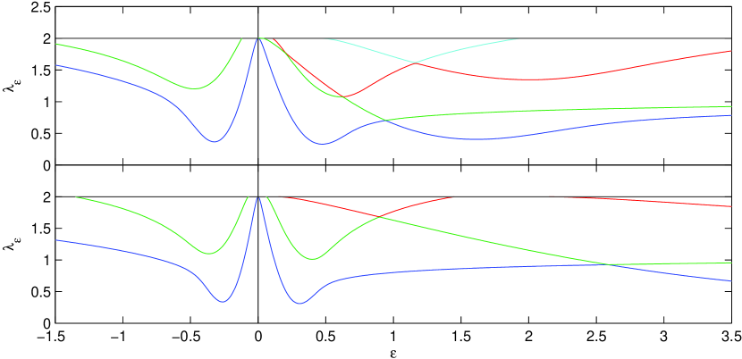
Figure 4: Dependence of eigenvalues on $\varepsilon$ in the critical case $\langle\beta\rangle=0$, $\tau>0$. Here $\alpha(x_{1})=\sqrt{2}-\varepsilon(x_{1}^{2}+bx_{1}-5)\exp(-x_{1}^{2}/10)$ and $d=2$. The upper figure corresponds to $b=1.5$, the lower one to $b=3.25$. All the crossings are avoided.

An answer to questions from (Q6) is provided by Figure 4. It corresponds to the critical case (B3) of Theorem 2 with $\beta(x_{1})=-(x_{1}^{2}+bx_{1}-5)\exp(-x_{1}^{2}/10)$, $\alpha_{0}=\sqrt{2}$, and $d=2$; the parameter $b$ changes the asymmetry of $\beta$. In addition to the weakly-coupled eigenvalue of Theorem 2, there are also other eigenvalues emerging from the continuous spectrum as $\varepsilon$ increases. The lower figure (case $b=3.25$) shows that there might be eigenvalues existing in disjunct intervals of $\varepsilon$ (the red curve). By diminishing $\alpha_{0}$ we can achieve the situation when there is only one eigenvalue with a similar behaviour: it emerges from the threshold of continuous spectrum (at $\varepsilon=0$), reaches a minimum, returns to the continuum, reappears later on, and returns finally to the continuum.

Another typical feature is that the energy levels do not cross. We saw always avoided crossings (at least in the unbroken $\mathcal{PT}$-regime), i.e. the order of levels remains unchanged and the non-monotonicity of the excited eigenvalues is preserved.

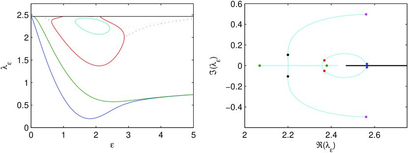
Figure 5: Broken $\mathcal{PT}$-symmetry. The left figure shows the dependence of eigenvalues on $\varepsilon$ in the case $\alpha(x_{1})=\pi/2-\varepsilon\exp(-x_{1}^{2}/10)$ and $d=2$. Here the dotted line is used to plot the real part of the eigenvalues if they form complex conjugate pairs instead of being real. The right figure shows the trajectory of a pair of (complex) eigenvalues in the complex plane. Here the thick black line marks the continuous spectrum. The pairs of dots show positions of eigenvalues for different values of $\varepsilon$: $0.1$ (blue), $1.3$ (red), $2.1$ (green), $2.5$ (black), and $8$ (magenta). An animation can be found at the website [19].

The spectrum in Figure 5 is remarkable from two points of view. First, it corresponds to the case of (Q2) from the end of Section 2, since the constant $\alpha_{0}$ is chosen so that its square coincides with the threshold of the continuous spectrum, which is $(\pi/2)^{2}\approx 2.47$ for $d=2$. Second, we see that this situation provides a negative answer to (Q5), i.e. the $\mathcal{PT}$-symmetry can be broken, and a partial answer to (Q7). Let us comment on the behaviour depicted by the cyan curve. There is a critical value of the parameter $\varepsilon$ for which there emerges a pair of complex conjugate eigenvalues from the continuous spectrum (we suspect that they emerge due to a collision of two embedded eigenvalues). As $\varepsilon$ increases, the eigenvalues propagate in the complex plane (this is indicated by the curves joining the blue and red dots in the right figure; the dotted curve in the left picture traces the common real parts of the eigencurves) till they collide on the real axis and become real. Then they move on the real axis (as the green dots) in opposite directions till they reach turning points (each of them for different value of $\varepsilon$), starts to approach each other, coalesce again and continue as a pair of complex conjugate eigenvalues (indicated by the black and magenta dots) until they disappear in the continuous spectrum. The behaviour of the eigenvalues depicted by the red curve in the left picture is more difficult in that one of them seems to have the turning point inside the continuous spectrum. Because of the collisions we see that the eigenvalues can actually be degenerate if the $\mathcal{PT}$-symmetry is broken, providing a positive answer to one of the questions from (Q6).

Let us mention that the behaviour of the eigenvalues in the regime of broken $\mathcal{PT}$-symmetry exhibits certain similarities with the over-damped phenomena as regards the spectrum of the infinitesimal generator of the semigroup associated with the damped wave equation [10, 11, 12]. This indicates the unifying framework of Krein spaces behind these two problems [20, 14].

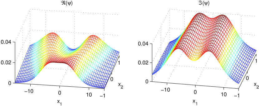
Figure 6: Real and imaginary parts of an eigenfunctions corresponding to the smallest (positive) eigenvalue of $H_{\alpha}$ for $\alpha(x_{1})=1/3-0.65\exp(-0.025x_{1}^{2})$.

In Figure 6, we present an example of eigenfunction corresponding to the case (B1) of Theorem 2. We check that the behaviour of the eigenfunction is in perfect agreement with the asymptotic results of Theorem 3.

Even if the corresponding eigenenergies are real, the non-Hermiticity prevents from choosing the eigenfunctions real. Since the latter is in particular true for the lowest eigenvalue, it does not make sense to speak about the super- and sub-harmonic properties of the corresponding eigenfunction (which hold in the self-adjoint case). However, although there is no variational characterization of eigenvalues in the present model, numerically we observe that the real and imaginary parts of the eigenfunction corresponding to the lowest eigenvalue are super-harmonic separately in the regime of unbroken $\mathcal{PT}$-symmetry. This follows, of course, from the observations that they do not change sign and that the spectrum is positive.

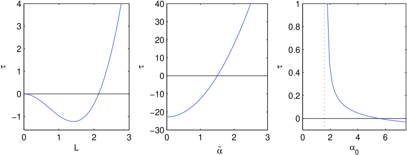
Figure 7: Dependence of $\tau$ on parameters defining $\alpha$ in the step-like situation of Section 3.1, with $d=2$. The first two figures deal with an antisymmetric square well in the regime $|\alpha_{0}|<\pi/d$, while the last one deals with a symmetric square well in the regime $\alpha_{0}>\pi/d$. The first (respectively second) figure shows the dependence of $\tau$ on the width $\pm L_{\pm}=:L$ (respectively on the coupling $\tilde{\alpha}$) for fixed $\alpha_{0}=1/3$ and $\alpha_{\pm}=\alpha_{0}\mp 1$ (respectively fixed $\alpha_{0}=1$, $\pm L_{\pm}=2$ and variable $\alpha_{\pm}=\alpha_{0}\mp\tilde{\alpha}$). In the last figure we show the dependence of $\tau$ on $\alpha_{0}$ for $L=10$ and variable $\alpha_{\pm}=(\alpha_{0}-1)$; here the dotted line corresponds to $\pi/d$.

Finally, in Figure 7 we visualize the dependence of the complicated quantity $\tau$ defined in (6) on various parameters. In particular, we see that it changes sign, giving a positive answer to (Q1). Consequently, all the cases of Theorem 2 for the critical case $\langle\beta\rangle=0$ and for the regime $|\alpha_{0}|>\pi/d$ can be achieved. We also see that the first figure is in qualitative agreement with an analytic result of [6, Prop. 2.1].

5 Conclusion

In this paper we tried to enlarge our knowledge of the point spectrum of a non-Hermitian $\mathcal{PT}$-symmetric operator introduced in [6] by analyzing it numerically. We confirmed theoretical results obtained in [6] by perturbation methods, and showed that they actually hold under much milder conditions about $\alpha$.

Besides this, it turned out that the operator can model a fairly wide range of situations. Indeed, its spectrum is very rich, and certain properties we found are unusual when we compare them with the standard self-adjoint cases. Among them we would like to point out the non-monotonic dependence on the strength of perturbation and the existence of the regime of broken $\mathcal{PT}$-symmetry. We hope that this study will stimulate further theoretical endeavour to extract and prove the salient features.

In particular, based on the present numerical analysis, we conjecture that there will be no other spectrum except for the continuous one if the parameter $\varepsilon$ is sufficiently large. At the same time, we were not able to find any discrete eigenvalues in the case of Corollary 1, i.e. (Q3) from the end of Section 2 seems to have a negative answer; the statement (v) of Theorem 1 would be trivial, then. Our numerical experiments also indicate that the condition mentioning in (Q2) is indeed just a technical hypothesis in Theorem 2.C, in the sense that it does not influence the existence/non-existence of weakly-coupled eigenvalues.

More generally, the existence of eigenvalues in the present model seems to have a nice heuristic explanation. We observe that the discrete spectrum behaves in many respects as that of a one-dimensional Schrödinger operator governed by the first-transverse-eigenvalue potential, i.e., $-\Delta+\min\{\alpha^{2},\pi^{2}/d^{2}\}$ in $L^{2}(\mathbb{R})$. Of course, this self-adjoint idealization is just approximative and cannot explain, in particular, the existence of non-real eigenvalues. However, it provides an insight into the non-monotonicity behaviour, the absence of point spectrum for large $\varepsilon$, the positivity of (the real part of) the spectrum, etc. It also formally explains the condition from the statement 1 (respectively 2) of Theorem 2.B, since this actually implies that the potential is attractive (respectively repulsive).

In this paper we were mainly interested in the eigenvalues emerging from the threshold $\mu_{0}^{2}$ of the continuous spectrum. A complete answer to the first question of (Q7) can be provided by a perturbation method similar to that of [6]. However, a more detailed analysis of the continuous spectrum would be still desirable. In particular, Figure 4 suggests that there can be embedded eigenvalues for larger values of the coupling parameter.

Finally, let us point out that the question of a direct physical motivation for the Hamiltonian $H_{\alpha}$ remains open. In this paper we were rather interested in consequences of the non-self-adjointness on spectral properties of this specific model in the context of $\mathcal{PT}$-symmetric quantum mechanics. On the other hand, motivated by problems in semiconductor physics, similar self-adjoint, respectively non-self-adjoint but dissipative, Robin-type boundary conditions has been considered recently in [15], respectively in [16]. In a different context, the present ($\mathcal{PT}$-symmetric) Robin-type boundary conditions imply that we actually deal with the Helmholtz equation in an electromagnetic waveguide with radiation/dissipative boundary conditions.

Acknowledgment

The authors are grateful to Denis Borisov for valuable discussions. The work has been supported by the Czech Academy of Sciences and its Grant Agency within the projects IRP AV0Z10480505 and A100480501, and by the project LC06002 of the Ministry of Education, Youth and Sports of the Czech Republic.

References

- [1] R. A. Adams, Sobolev spaces, Academic Press, New York, 1975.
- [2] S. Albeverio, S.-M. Fei, and P. Kurasov, Point interactions: -Hermiticity and reality of the spectrum, Lett. Math. Phys. 59 (2002), 227–242.
- [3] C. M. Bender, Making sense of non-Hermitian Hamiltonians, Rep. Prog. Phys. 70 (2007), 947–1018.
- [4] C. M. Bender and P. N. Boettcher, Real spectra in non-Hermitian Hamiltonians having symmetry, Phys. Rev. Lett. 80 (1998), no. 24, 5243–5246.
- [5] D. Borisov, Discrete spectrum of a pair of non-symmetric waveguides coupled by a window, Sbornik Mathematics 197 (2006), no. 4, 475–504.
- [6] D. Borisov and D. Krejčiřík, -symmetric waveguide, preprint on arXiv:0707.3039 [math-ph] (2007).
- [7] E. Caliceti, F. Cannata, and S. Graffi, Perturbation theory of -symmetric Hamiltonians, J. Phys. A 39 (2006), 10019–10027.
- [8] E. Caliceti, S. Graffi, and J. Sjöstrand, Spectra of PT-symmetric operators and perturbation theory, J. Phys. A 38 (2005), 185–193.
- [9] , PT-symmetric non-self-adjoint operators, diagonalizable and non-diagonalizable, with a real discrete spectrum, J. Phys. A: Math. Theor. 40 (2007), 10155–10170.
- [10] S. Cox and E. Zuazua, The rate at which energy decays in a damped string, Comm. Partial Differential Equations 19 (1994), 213–243.
- [11] P. Freitas, Spectral sequences for quadratic pencils and the inverse spectral problem for the damped wave equation, J. Math. Pures Appl. 78 (1999), 965–980.
- [12] P. Freitas and D. Krejčiřík, Damped wave equation in unbounded domains, J. Differential Equations 211 (2005), no. 1, 168–186.
- [13] R. Gadyl’shin, On regular and singular perturbation of acoustic and quantum waveguides, Comptes Rendus Mechanique 332 (2004), no. 8, 647–652.
- [14] B. Jacob, C. Trunk, and M. Winklmeier, Analyticity and Riesz basis property of semigroups associated to damped vibrations, Journal of Evolution Equations, to appear; preprint on arXiv:math/0703247v1 [math.SP] (2007).
- [15] M. Jílek, Straight quantum waveguide with Robin boundary conditions, SIGMA 3 (2007), 108, 12 pages.
- [16] H.-Ch. Kaiser, H. Neidhardt and J. Rehberg, Macroscopic current induced boundary conditions for Schrödinger-type operators, Integral Equations and Operator Theory 45 (2003), 39–63.
- [17] M. Klaus, On the bound state of Schrödinger operators in one dimension, Ann. Phys. 108 (1977), 288–300.
- [18] D. Krejčiřík, H. Bíla, and M. Znojil, Closed formula for the metric in the Hilbert space of a -symmetric model, J. Phys. A 39 (2006), 10143–10153.
-
[19]
D. Krejčiřík and M. Tater,
http://gemma.ujf.cas.cz/~david/KT.html. - [20] H. Langer and Ch. Tretter, A Krein space approach to PT-symmetry, Czech. J. Phys. 54 (2004), 1113–1120.
- [21] G. Lévai, Solvable -symmetric potentials in higher dimensions, J. Phys. A: Math. Theor. 40 (2007), F273–F280.
- [22] G. Lévai and M. Znojil, Systematic search for -symmetric potentials with real energy spectra, J. Phys. A 33 (2000), 7165–7180.
- [23] A. Mostafazadeh, Pseudo-Hermiticity versus PT symmetry: The necessary condition for the reality of the spectrum of a non-Hermitian Hamiltonian, J. Math. Phys. 43 (2002), 205–214.
- [24] F. G. Scholtz, H. B. Geyer, and F. J. W. Hahne, Quasi-Hermitian operators in quantum mechanics and the variational principle, Ann. Phys 213 (1992), 74–101.
- [25] M. S. Swanson, Transition elements for a non-Hermitian quadratic Hamiltonian, J. Math. Phys. 45 (2004), 585–601.
- [26] J. A. C. Weideman and S. C. Reddy, A MATLAB differentiation matrix suite, ACM Trans. Math. Software 26 (2000), 465–519.
- [27] M. Znojil, -symmetric square well, Phys. Lett. A 285 (2001), 7–10.