Distribution of an Ohmic current in the close vicinity of a quantum point contact

Abstract

We present the essential findings of the screening theory of the integer quantum Hall effect (IQHE) considering a quantum point contact (QPC). Our approach is to solve the Poisson and the Schrödinger equations self-consistently, taking into account electron interactions, within a Hartree type approximation for a two dimensional electron gas (2DEG) subject to high perpendicular magnetic fields. The Coulomb interaction between the electrons separates 2DEG into two co-existing regions, namely quasi-metallic compressible and quasi-insulating incompressible regions, which exhibit peculiar screening and transport properties. In the presence of an external current, we show that this current is confined into the incompressible regions where the drift velocity is finite. In particular, we investigate the distribution of these incompressible strips and their relation with the quantum Hall plateaus considering a quasi 1D constriction, i.e. a QPC.

1 Introduction

The increasing amount of interest in quantum information processing attracted many experimentalists and theoreticians to investigate the transport properties of low dimensional charge systems. Beyond interest to build quantum computational units, i.e. q-bits, and the calculation algorithms which are supposed to be used by these units, the coherency of the information processing, or in other words information transport, is an essential challenge. Since some of the proposed units are defined on the 2DEG, the information carriers are naturally the electrons. In the absence of an external magnetic field, the well-known and well-defined Landauer channels [1] are the best candidates for coherent transport. These channels are by definition ballistic and 1D. They are formed due to the size quantization of the system under investigation. A similar non-interacting single particle picture commonly used to describe the transport, also in the presence of an external magnetic field, is the so-called Landauer-Büttiker edge states (LB-ES) [2]. However, its relevance in explaining some of the recent quantum Hall, in particular the local probe, experiments is questionable, where the importance of electron-electron ($e-e$) interaction is shown to be dominant [3, 4, 5]. The simplest way of including $e-e$ interactions is the so-called electrostatic approximation (ESA) which is based on the Landau quantization introduced by the external magnetic field [6]. In this approach, the 2DEG is split into two regions depending on the value of the Fermi energy with respect to Landau level energy, $E_{n}=\hbar\omega_{c}(n+1/2)$, where $\omega_{c}=eB/m^{*}$ is the cyclotron frequency and $m^{*}$ is the effective mass of the electron ($=0.067m_{e}$), with Landau index $n$. If the Fermi energy equals one of the Landau energies, which has a $2\pi l^{2}-$fold degeneracy, the electronic system is quasi-metallic so-called compressible and screening is nearly perfect. Otherwise, when the Fermi energy lies in between two consequent Landau levels, screening is poor and system is called to be incompressible. Beyond the differences in their screening properties, the transport properties of compressible and incompressible regions are different as black and white. First of all we should mention that, within a compressible strip (CS) the screened potential is (ideally) flat and density is varying, as a result of high density of states (DOS) at the Fermi energy, whereas within the incompressible strip (IS) the potential is varying (since the external potential could not be screened perfectly) and electron density is constant (see Fig. 1). The discussion on ”where the current flows ?” is a long lasting question. As early as, the formation of CS/ISs was realized, it was conjectured that, the current should flow from the IS, since the screened potential has a gradient only within these regions [7, 8] and back scattering is suppressed [9, 10, 11]. However, later it was argued that since there are no states available at the Fermi energy the current should flow from the CSs, where it is possible to generate an excitation [6, 12]. Moreover, the non-interacting limit of the CS was claimed to reduce to the Landauer-Büttiker formalism [12]. The recent local potential [13] and transparency [4] experiments supported the findings of the first model, where it was shown that the positions of the Hall potential drops coincide with the predicted positions of the (innermost) ISs within ESA. Even before the ESA, a self-consistent interaction model was developed by R.R. Gerhardts and his co-workers [14], which excellently agrees with the experimental results after including the influence of an imposed current [9, 10]. In this model, a Hartree type mean-field approximation was considered, which provides the local distribution of the electron density and potential profiles as a function of magnetic field and temperature [15, 16, 17]. A local transport model was incorporated to describe the current distribution, where the entries of the conductivity tensor were calculated from a reasonable conductivity model, e.g. self-consistent Born approximation (SCBA) [18], provided that local electron distribution is known. Moreover, the position dependent electrochemical potential, thereby the local current distribution, was obtained within a local version of the Ohm’s law under the condition of a local equilibrium [9, 19]. This self-consistent theory was implemented to many interesting 2DEG systems successfully explaining the relevant experiments [20, 21, 22, 23, 24, 25].

The recent quantum interference experiments considering 2DES under strong magnetic fields, provided unexpected information on the transport electrons. In the Mach-Zehnder interference setups [26, 27, 28, 29], it was observed that the contrast in the interference oscillations (visibility) is path-length independent, which is in strong contradiction with the optical counterpart of the experimental setup. The basic idea is to split a monochromatic (mono-energetic) light (electron) beam from a half-transparent mirror (QPC) and measure the interference after these two split beams interfere. In these experiments the LB-ES are assumed to simulate the light beam and QPCs to replace the mirrors. However, the out come of the experiments were not easy to explain within a naive single particle model, without many assumptions [30, 31]. Another very interesting experiment concerning QPCs is performed at the Westervelt group (Harvard), where a local probe technique is used to observe electron flow near a QPC [32]. There it was clearly shown that the actual realization of the sample is dominant in determining the transport taking place (see the paper by T. Kramer within this issue). The essential physics was explained comprehensively within the wave-packet formalism at relatively low magnetic fields ($\sim 0.4$ T), where one should not expect the formation of the incompressible strips. However, if one considers higher magnetic fields one should in principle include the effect of $e-e$ interactions in a self-consistent manner. Beyond the interference experiments, the transmission measurements performed at a 2DEG using a single QPC has shown peculiar effects [33]. The suppression or enhancement of the transmission amplitude presents significant deviation from the chiral Luttinger liquid model [34], meanwhile this effect could be explained by considering an electron-hole asymmetry [35]. In this treatment the formation of a large incompressible region is assumed, however, the $e-e$ interaction is not taken into account.

Here we provide, such a calculation scheme within Thomas-Fermi approximation. In Sec. 2 we briefly describe the self-consistent model to obtain the electrostatic quantities and discuss the limitations of this approach. We then proceed with the formulation of the current flow within a local Ohm’s law in Sec.  3. We finalize, our work by showing the interrelation between the quantized Hall plateaus (QHP) and the expected distribution of the IS, and thereby local current, near a QPC, also in the out of linear response regime.

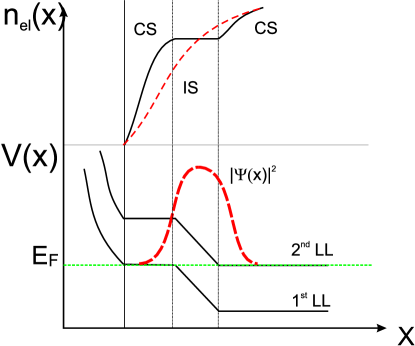
Figure 1: A sketch of the density profile as a function of lateral coordinate (upper panel) and the corresponding energy dispersion, i.e. 1^st and 2^nd Landau levels (lower panel). The vertical dashed lines indicate the region where the incompressible strip (IS) resides, whereas the horizontal line in the lower panel is the Fermi energy. The dashed curve in the upper panel is the density distribution, when one considers finite extend of the wave function (dashed (green) curve in the lower panel) and the corresponding curve calculated within the TFA.

2 The electrostatic self-consistency

The essential physics of a 2DEG subject to strong perpendicular magnetic field is governed by the single particle Hamiltonian

$$H=H_{0}+V(x,y)$$ (1)

with the kinetic term

$$H_{0}=\frac{1}{2m^{*}}(\textbf{p}-\frac{e}{c}\textbf{A})^{2}$$ (2)

where p stands for momentum and A for the vector potential. The potential energy is composed of the external $V_{\rm ext}(x,y)$ and interaction $V_{\rm H}(x,y)$ terms

$$V(x,y)=V_{\rm ext}(x,y)+V_{\rm H}(x,y).$$ (3)

Using a relevant gauge (here we use the Landau gauge to exploit the symmetry of the system) and assuming a translational invariance, one ends with the reduced 1D Hamiltonian in $x-$ direction, which is nothing but a Harmonic oscillator centered at $X=-l^{2}k_{y}$. The solutions of the Hamiltonian in $y-$ direction are properly normalized plane waves with quasi-continuous momentum $k_{y}$ $(=\frac{n\pi}{L_{y}}$, where $L_{y}$ is the sample length), and $l^{2}=\hbar/m\omega_{c}$ is the square of the magnetic length. By translational invariance we mean that, the quantization effects arising from the finite length of the sample are negligible. The solution of the Schrödinger equation in $x-$ direction results in the well-known Landau wave functions

$$\Phi_{n_{X}}(x)=\frac{1}{\sqrt{2^{n}n!\sqrt{\pi}l}}\exp{[-(\frac{x-X}{l})^{2}/2]}\times H_{n}(\frac{x-X}{l}),$$ (4)

where $n$ is the Landau index and $H_{n}(\xi)$ the $n$th order Hermite polynomial with the argument $\xi$, whereas the eigen energies are

$$E_{n,X}=\hbar\omega_{c}(n+1/2).$$ (5)

The external potential is obtained by solving the 3D Poisson equation [36, 37] for the structure shown in Fig.2a. The calculation scheme and its details of implementing to a QPC is far beyond the scope of this paper and is discussed elsewhere, however, the for the present work a reasonable confinement potential profile is sufficient to initialize the self-consistent scheme described below. The Hartree potential is defined from the electron distribution via,

$$V_{\rm H}(x,y)=\frac{2e^{2}}{\bar{\kappa}}\int_{A}K(x,y,x^{\prime},y^{\prime})n_{\rm el}(x^{\prime},y^{\prime})dx^{\prime}dy^{\prime},$$ (6)

where the kernel $K(x,y,x^{\prime},y^{\prime})$ gives the solution of the Poisson equation at $(x,y)$ for a point charge residing at the point $(x^{\prime},y^{\prime})$, assuming periodic boundary conditions in 2D and $\bar{\kappa}$ is an average dielectric constant defined by the sample parameters. Once the Hamiltonian given in Eq. 1 is solved one can obtain the electron density from,

$$n_{\rm el}(x,y)=\sum_{n,k_{y}}{|\psi_{n,k_{y}}(x,y)|^{2}}f(E_{n,k_{y}}-\mu^{*}),$$ (7)

where f(E) is the Fermi function and $\mu^{*}$ is the (position dependent, in the presence of an external current) electrochemical potential.

We first make the assumption that, the total potential varies smoothly on the scale of the magnetic length, i.e. Thomas-Fermi approximation (TFA). This allows us to replace the wave functions with delta functions, the eigen energies are then given by:

$$E_{n}(X,y)=E_{n}+V(X,y).$$ (8)

The above approximation results in a simpler description of the electron density,

$$n_{\rm el}(x,y)=\int{dEf(E-\mu^{*})D(E,(x,y))}$$ (9)

within the TFA, where $D(E,(x,y))$ stands for the local density of states (LDOS). It is more common to use the filling factor $\nu(x,y)$ instead of the electron density, which is defined as $\nu(x,y)=2\pi l^{2}n_{\rm el}(x,y)$. The name itself is explanatory, filling factor describes how many of the low-lying Landau levels is filled. If it is a integer, it means that all the states below the Fermi level are occupied (i.e. incompressible), otherwise show how much of the top most Landau level has available states.

The calculation procedure is as follows, we start with a given external potential generated by the donors and gates, then calculate the electron density distribution in the absence of an external magnetic field. The average electron density, $\overline{n_{\rm el}}=\int_{A}{n_{\rm el}(x,y)}$, is kept constant all through the calculation, which enables to have a convergence criteria. This electron density initializes the potential given in Eq.6, which in turn determines the electron density via Eq.9. The numerical procedure is a bit more complicated than described, however, the details can be found in Ref. [22, 38].

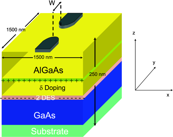
Figure 2: Schematic draw of the sample under investigation. The gates defining the QPC are deposited on the surface of the sample along $y-$ direction with a separation $W\sim 150$ nm, under a potential bias $V_{\rm g}=-1.5$ V, such that the 2DEG beneath is depleted. The width of the gates are $\sim 500$ nm and assumed to be thinner than 10 nm. A homogeneous donor layer with a number density $4\times 10^{12}$ cm^-2 is laying 43 nm below the surface, which donates almost 10 percent of its excess electrons to the 2DEG. The resulting electron density of the 2DEG is $3.0\times 10^{11}$ cm^-2 without gates. In order to satisfy the open boundary conditions a larger lattice is considered in actual calculations spanned with $128\times 128\times 32$ mesh points in $x$, $y$ and $z$ directions, respectively.

Before proceeding with the discussion of the self-consistent results obtained for a QPC geometry, we would like to make some comments on the weak points of the TFA. The first issue is that, if an IS becomes narrower than the magnetic length our approximation fails [17, 10]. Such a potential profile is shown in Fig. 1, therefore one should avoid these situations and perform a spatial averaging over the magnetic length both for the density and the potential profiles as a first order approximation [10]. This approach has been used previously for these systems and is shown to be sufficiently powerful to simulate the effect of the quantum mechanical wave functions [39, 21]. Another issue about narrow ISs, is that the LDOS ($D(E,(x,y)$) become broader, when considering steep potential drops, i.e. large transverse electric fields [40]. Due to this local broadening of the LDOS the Landau gap is smeared out and as a result IS disappears [41]. These two observations together, i.e. overlap of the wave functions and local broadening, justifies the validity of performing a spatial average over magnetic length or even over the Fermi wavelength $\lambda_{F}$, which we also will perform through out this work.

The sample that we investigate is shown in Fig. 2, a multi-layer GaAs is grown on top of the substrate, which is followed by a thick layer of AlGaAs. This layer is ($\delta$-) doped by Silicon, which provide electrons to the 2DEG formed at the interface of the two different materials. On top of the sample (metallic) gates are patterned to manipulate the electron density at the 2DEG. If a sufficiently large negative potential is applied to these gates (here patterned as a QPC) the electrons underneath the gates are depleted, however, the potential profile satisfies the conditions of the TFA [37, 38]. We will consider a geometric pattern of the gates such that the opening of the QPC is 150 nm and is smooth again on the length scales of the magnetic length.

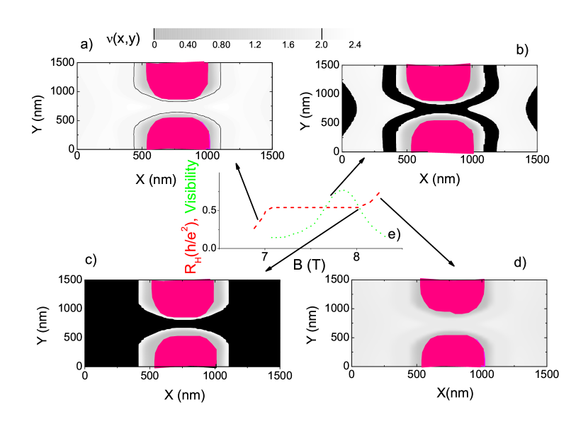
Figure 3: Spatial distribution of the electron density (a-d) together with an illustrative sketch of the Hall resistance (broken red line) and the expected visibility (dotted green line) as a function of magnetic field strength (e). The solid black regions indicate an integer filling factor equal to 2, i.e. an IS, whereas the degrading gray scale denotes the compressible regions with varying electron density, whereas the colored (pink) region is the electron depleted region. The initial potential calculated at $B=0$ is obtained for a geometry shown in Fig. 2. The characteristic $B$ values are chosen depending on the existence and the width of the ISs, such that the resulting magnetic field strengths are $B=6.7$ T (a), $B=7.7$ T (b), $B=7.9$ T (c), $B=8.3$ T (d). All the calculations are done at temperatures satisfying $k_{B}T/\hbar\omega_{c}\ll 0.04$ for $I=0$. For the DOS broadening parameter see the related text.

Fig.  3 shows a sequence of density distributions calculated at selected magnetic field values, for which the 2DEG system is out of the $\nu=2$ QHP at low $B$ fields (a), at the lower edge of the QHP (b) at the higher edge of the QHP (c) out of the QHP at high $B$. Pedagogically, it is preferable to start the discussion considering high magnetic fields since the density distributions at $B=0$ and at strong $B$ are similar. At zero magnetic field a 2DEG is known to be quasi-metallic, due to high (but not infinite) DOS, screening is perfect and the external potential is almost flat in the interior of the sample. The situation is similar at high magnetic fields, since only the lowest (spin degenerate) Landau level is partially occupied, hence the system acts as a metal and external potential is almost perfectly screened. However, decreasing magnetic field explicitly implies that the degeneracy $(\sim l^{-2})$ is also reduced therefore the lowest Landau level can not accommodate all the electrons. This essentially means that the Fermi energy of the system lies between two consequent Landau levels all over the sample, this situation corresponds to Fig. 3c. Now, once the higher Landau level is being occupied the $e-e$ interaction forces the system to establish an electrostatic equilibrium by minimizing the energy. Therefore the IS become narrower and higher filling fractions are present, Fig. 3b. Even lowering the degeneracy, these IS become more and more narrow until their widths become smaller or comparable with the quantum mechanical length scales as observed in Fig 1.

These results point out clearly that even in a single QHP the edge states exhibit different behavior by changing their widths. Moreover, at a very clean sample (where no long-range potential fluctuations are present) the coherence of the edge state is lost due to averaging of the phase. On the other hand, if an IS is well separated and sufficiently wide, it will become “more” coherent. This is true, if the current is confined to these regions, which we will demonstrate in the next section. We should also remind that our classical approach in defining the current disables us to define a phase coherent transport in the sense of LB-ES. Although there are attempts in defining a coherent transport including spin-orbit coupling, due to large Zeeman splitting the arguments of this model [42] are rather energetically irrelevant. However, our hand waving arguments coincides with the findings of most recent Mach-Zehnder experiments [43], where the amplitude of the visibility is measured as a function of applied magnetic field. The reduction of this amplitude is observed at the higher and the lower edge of the QHP, meanwhile a local maxima occurred closer to the higher edge.

3 The local Ohm’s law and its implication

In this section we briefly summarize the previously developed local Ohm’s law applied to a 2DEG under quantized Hall conditions. This model assumes that the Ohm’s law is valid on the scales larger than the Fermi wavelength and a local equilibrium is established. It is essentially based on the argument that if the local potential and electron distribution is known one can calculate the local current distribution with in the linear response regime, i.e. at very small currents.

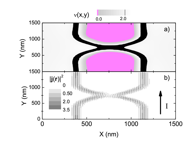
Figure 4: Gray scale plot of the density (a) and current distribution within the $\nu=2$ quantized Hall plateau. An electric field is applied in the $y-$ direction resulting a fixed current ($j({\bf r})=j_{0}(0,0.1)$), where the 1D current density is set to $-1.05\times 10^{-2}$ A/m. All the other parameters are the same as Fig. 3 for $B=7.2$ T.

The local Ohm’s law assumes that the relation

$$\textbf{E}(\textbf{r})=\hat{\rho}(\textbf{r}).\textbf{j}(\textbf{r})$$ (10)

is valid locally, i.e on the scales of the Fermi wavelength. The next step is to satisfy the Maxwell equation

$$\bf{\nabla}\times\textbf{E}(\textbf{r})=0$$ (11)

and the equation of continuity

$$\bf{\nabla}\cdot\textbf{j}(\textbf{r})=0$$ (12)

simultaneously, for a stationary situation. From the above equations one can obtain the local current distribution, if the local resistivity tensor is known for an external fixed current

$$I=\int_{A}{\textbf{j}(\textbf{r})d\textbf{r}}.$$ (13)

Here, we assume that $\hat{\rho}(\textbf{r})$ is nothing but the inverse of the conductivity tensor which is related to the electron distribution via some reasonable conductivity model. For consistency reasons we assume a Gaussian broadened spectral function

$$A_{n}(E)=\frac{e^{(-[\frac{E_{n}-E}{\Gamma}]^{2})}}{\sqrt{\pi}\Gamma},$$ (14)

where $\Gamma$ is the broadening parameter defined by the impurity potential, which we set $\Gamma/\hbar\omega_{c}=0.3$ in order to smear out the narrow ISs. For the given spectral function the longitudinal conductivity is calculated as

$$\sigma_{l}=\frac{2e^{2}}{h}\int_{-\infty}^{\infty}dE\large[-\frac{\partial f}{\partial E}\large]\sum_{n=0}^{\infty}\left(n+\frac{1}{2}\right)[e^{(-[\frac{E_{n}-E}{\Gamma_{\rm imp}}]^{2})}]$$ (15)

whereas the Hall conductivity is simply the Drude result

$$\sigma_{H}=\frac{2e^{2}}{h}\nu.$$ (16)

One can already see the essence of the local model related with the existence of the ISs: the longitudinal conductivity vanishes if the filling factor is an integer, which is the case when considering an IS. This is a result of the Landau gap, if the Fermi energy lies in between two Landau levels there are no available states at the Fermi level. Therefore, the conductivity and consequently the longitudinal resistivity vanishes:

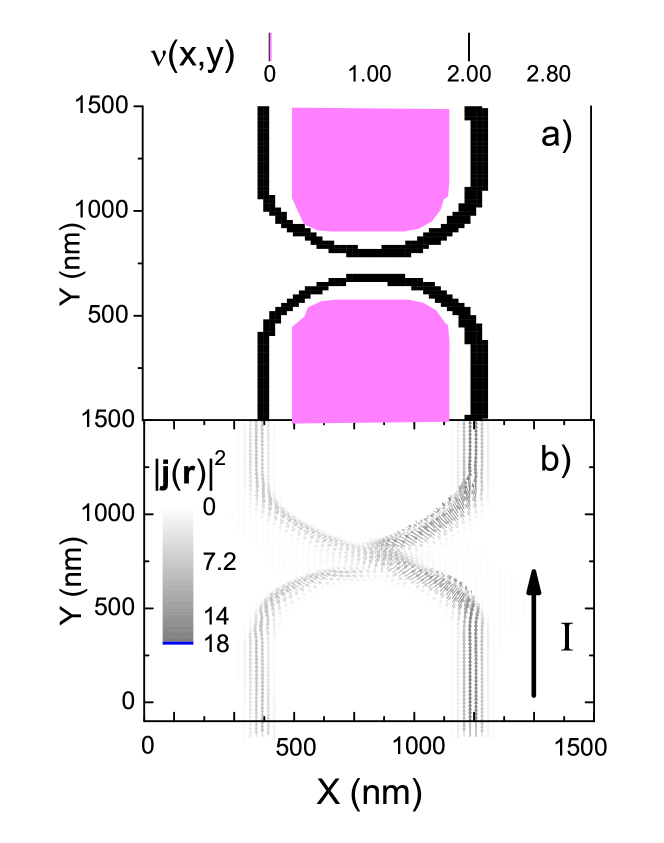
Figure 5: Gray scale plot of the electron (a) and current density (b), considering a sufficiently large current density, $-4.20\times 10^{-2}$ A/m, considering $B=7.2$ T. The Asymmetry is induced by this current is significant on the righthand side of the sample.

$$\rho_{l}(x,y)=\frac{\sigma_{l}(x,y)}{\sigma^{2}_{l}(x,y)+\sigma^{2}_{H}(x,y)}=\frac{0}{0^{2}+\sigma_{H}^{2}}=0.$$ (17)

In the linear response regime we assume that the relation

$$V((x,y);I)-V((x,y);0)\approx\mu^{*}((x,y);I)-\mu^{*}_{\rm eq},$$ (18)

holds, i.e. the imposed external current does not change the density and potential profile, thereby the position dependent electrochemical potential can still be considered as constant. In Fig.4 we plot the current distribution corresponding to a density distribution shown in Fig.3. It is apparent that the current is confined to the regions where a well-developed IS is present. Therefore, at least in the linear response regime, once the spatial distribution of the ISs is obtained the current distribution can be calculated mutually. However, when the imposed current is strong enough to influence the density distribution, one should calculate the position dependent electrochemical potential $\mu^{*}(\textbf{r})$ via

$$E(\textbf{r})=\nabla\mu^{*}(\textbf{r})/e.$$ (19)

This relation brings a new set of self-consistent equations, which have to be solved numerically. In our (numerical) calculation scheme, we start with a small total current and in each iteration step increase the strength of $I$ slowly so that a convergence is guaranteed. The details of the calculation is given elsewhere [37].

The density and current distribution is shown in Fig.5 for a situation where the external current is sufficiently large. We observe that, the IS on the right side of the QPC is relatively larger than the one of at the left side. The physics leading to this effect is rather simple: when an external current is driven, a Hall potential is built which tilts the Landau levels, therefore the electrons have to compensate this potential change. However, one can not add more electrons to the IS since there are no states available. The only way to screen the Landau tilting is to increase the widths of the ISs on one side where the Hall potential is larger [9, 19]. This effect clearly demonstrates the importance of $e-e$ interactions. Without the self-consistent treatment one would only get a higher chemical potential one one side, however, the widths of the edge channels would remain unchanged. The asymmetry induced by the large external current on the widths of the IS is also observed in the local probe experiments, which is a strong evidence that our model of local Ohm’s law is relevant to explain the edge physics of the IQHE.

4 Summary

In conclusion we have demonstrated that the spatial distribution of the current carrying incompressible strips vary depending on the magnetic field strength considering a quantum point contact induced at a 2DEG. Therefore, in interpreting the experimental results one should keep in mind that the so-called edge states may present different transport and coherency properties even within a single quantum Hall plateau. Our electrostatic model relies on the self-consistent solution of the Poisson and Schrödinger equations using numerical techniques. We have explicitly shown that the $e-e$ interactions result in the formation of incompressible and compressible regions. Based on the overlap of the quantum mechanical wave functions and the local broadening of the DOS within the incompressible strips, which has an extend smaller or comparable to the Fermi wavelength, we performed a spatial average over $\lambda_{\rm F}$ to cure the artifacts of the TFA. The second set of self-consistent equations has been introduced to obtain the current distribution, namely solving the Maxwell equation and equation of continuity simultaneously. In the small current regime, we have shown that the current is confined to the incompressible strips since the back scattering is suppressed and the longitudinal resistivity vanishes. Meanwhile, the Hall resistivity assumes its quantized value. We have also shown that, considering sufficiently large external currents induces an asymmetry both in the density and in the current distribution, which we think is an interesting issue to check with the experiments. The author would like to thank R.R. Gerhardts for his initiation, supervision and contribution in developing the model, S. Arslan and A. Weichselbaum in providing the data concerning the solution of the 3D Poisson equation and D. Eksi and S. Aktas for all their contribution in the improvement of the numerical code. The enlightening discussions with V. Golovach is also highly appreciated. This work was supported by the NIM Area A and SFB 631.

References

References

- [1] R. Landauer, Phys. Lett. 85A, 91 (1981).
- [2] M. Büttiker, Phys. Rev. Lett. 57, 1761 (1986).
- [3] E. Ahlswede, P. Weitz, J. Weis, K. von Klitzing and K. Eberl, Physica B 298, 562 (2001).
- [4] S. Ilani, J. Martin, E. Teitelbaum, J. H. Smet, D. Mahalu, V. Umansky and A. Yacoby, Nature 427, 328 (2004).
- [5] J. Horas, A. Siddiki, W. Wegscheider and S. Ludwig, cond-mat/0707.1142, to appear in Physica E (2007).
- [6] D. B. Chklovskii, B. I. Shklovskii and L. I. Glazman, Phys. Rev. B 46, 4026 (1992).
- [7] A. M. Chang, Solid State Commun. 74, 871 (1990).
- [8] M. M. Fogler and B. I. Shklovskii, Phys. Rev. B. 50, 1656 (1994).
- [9] K. Güven and R. R. Gerhardts, Phys. Rev. B 67, 115327 (2003).
- [10] A. Siddiki and R. R. Gerhardts, Phys. Rev. B 70, 195335 (2004).
- [11] S. Kanamaru, H. Suzuuara and H. Akera, J. Phys. Soc. Jpn. 75, (2006), and proceedings EP2DS-14, Prague 2001.
- [12] C. W. J. Beenakker, Phys. Rev. Lett. 62, 2020 (1989).
- [13] E. Ahlswede, J. Weis, K. von Klitzing and K. Eberl, Physica E 12, 165 (2002).
- [14] U. Wulf, V. Gudmundsson and R. R. Gerhardts, Phys. Rev. B 38, 4218 (1988).
- [15] K. Lier and R. R. Gerhardts, Phys. Rev. B 50, 7757 (1994).
- [16] J. H. Oh and R. R. Gerhardts, Phys. Rev. B 56, 13519 (1997).
- [17] T. Suzuki and T. Ando, J. Phys. Soc. Jpn. 62, 2986 (1993).
- [18] T. Ando, A. B. Fowler and F. Stern, Rev. Mod. Phys. 54, 437 (1982).
- [19] A. Siddiki, D. Eksi, E. Cicek, A. I. Mese, S. Aktas and T. Hakioglu, cond-mat/0707.1229, to appear in Physica E (2007).
- [20] A. Siddiki, S. Kraus and R. R. Gerhardts, Physica E 34, 136 (2006).
- [21] A. Siddiki, Phys. Rev. B 75, 155311 (2007).
- [22] A. Siddiki and F. Marquardt, Phys. Rev. B 75, 045325 (2007).
- [23] D. Eksi, E. Cicek, A. I. Mese, S. Aktas, A. Siddiki and T. Hakioglu, Phys. Rev. B 76, 075334 (2007).
- [24] P. M. Krishna, A. Siddiki, K. Guven and T. Hakioglu, cond-mat/0707.1228, to appear in Physica E (2007).
- [25] A. Siddiki, E. Cicek, D. Eksi, A. I. Mese, S. Aktas and T. Hakioglu, cond-mat/0707.1244, to appear in Physica E (2007).
- [26] Y. Ji, Y. Chung, D. Sprinzak, M. Heiblum, D. Mahalu and H. Shtrikman, Nature 422, 415 (2003).
- [27] I. Neder, M. Heiblum, Y. Levinson, D. Mahalu and V. Umansky, Phys. Rev. Lett. 96, 016804 (2006).
- [28] L. V. Litvin, H.-P. Tranitz, W. Wegscheider and C. Strunk, Phys. Rev. B 75, 033315 (2007).
- [29] L. V. Litvin, A. Helzel, H. . Tranitz, W. Wegscheider and C. Strunk, ArXiv e-prints 802, (2008).
- [30] P. Samuelsson, E. Sukhorukov and M. Buttiker, Phys. Rev. Lett. 92, 026805 (2004).
- [31] I. Neder and F. Marquardt, New Journal of Physics 9, 112 (2007).
- [32] K. E. Aidala, R. E. Parrott, T. Kramer, E. J. Heller, R. M. Westervelt, M. P. Hanson and A. C. Gossard, Nature Physics 3, 464 (2007).
- [33] S. Roddaro, V. Pellegrini, F. Beltram, L. N. Pfeiffer and K. W. West, Physical Review Letters 95, 156804 (2005).
- [34] S. D. Sarma and A. Pinczuk, in Perspectives in Quantum Hall Effects (Wiley, New York, 1997).
- [35] S. Lal, ArXiv e-prints 709, (2007).
- [36] A. Weichselbaum and S. E. Ulloa, Phys. Rev E 68, 056707 (2003).
- [37] S. Arslan, A. Weichselbaum, D. Eksi, S. Aktas and A. Siddiki, in preperation .
- [38] S. Arslan, Dissertation, Technical University of Munich, 2008.
- [39] A. Siddiki and R. R. Gerhardts, Int. J. Mod. Phys. B 18, 3541 (2004).
- [40] T. Kramer, International Journal of Modern Physics B 20, 1243 (2006).
- [41] A. Siddiki and T. Kramer, in preperation (2008).
- [42] T. Hakioglu, Unpublished (2007).
- [43] P. Roulleau, F. Portier, D. C. Glattli, P. Roche, A. Cavanna, G. Faini, U. Gennser and D. Mailly, ArXiv e-prints 710, (2007).