Zonal Velocity Bands and the Solar Activity Cycle

Abstract

We compare the zonal flow pattern in subsurface layers of the Sun with the distribution of surface magnetic features like sunspots and polar faculae. We demonstrate that in the activity belt, the butterfly pattern of sunspots coincides with the fast stream of zonal flows, although part of the sunspot distribution does spill over to the slow stream. At high latitudes, the polar faculae and zonal flow bands have similar distributions in the spatial and temporal domains.

1 Introduction

The pattern of temporal variations in the solar differential-rotation rates discovered by Howard and LaBonte (1980) from the Mt. Wilson full-disc Dopplergram data is known as torsional oscillations. These manifest themselves as alternating latitudinal bands of slightly faster and slower than the average rotation velocities migrating from pole to the Equator in about 22 years. The low velocity of 3 – 5 m s^-1 of these zonal flows makes it difficult to detect them from the global rotation signal which is more than two orders of magnitude stronger, and it was remarkable that Howard and LaBonte were able to isolate these weak signals. The close correspondence between the torsional oscillation pattern and the surface magnetic-flux distribution in the sunspot latitudes led Howard and LaBonte (1980) to conclude that this velocity field is perhaps, the signature of a “large-scale deep-seated phenomenon” and that “this velocity field is associated in some way with the subsurface magnetic fields that are responsible for the solar cycle”.

A subsequent investigation by Snodgrass and Howard (1985) used the corrected values for the coefficients $A$, $B$, and $C$ of the parabolic fit for the global rotation to show that the full torsional oscillation pattern is not in the form of a continuous wave running from poles to the Equator but rather consisted of a high-latitude and a low-latitude branch with a break around 40 – $50^{\circ}$ with each of the two components consisting of a fast and a slow stream alternating with each other in time. Snodgrass and Howard (1985) also noticed that the low-latitude stream of enhanced shear that lies in between the fast zone and its poleward adjacent zone spatially coincides with the centroid of the sunspot distribution. Later, Snodgrass (1987, his Figure 2) in addition to confirming the overlap of the shear enhanced pattern with the sunspot distribution (referred to as the Butterfly pattern) for cycles 20 and 21, demonstrated that the zone of diminished shear is located in between the two successive sunspot activity zones, i.e., in between two successive butterfly patterns. This figure also showed that there are no magnetic features corresponding to the shear increase and decrease zones at latitudes beyond $\pm 60^{\circ}$. Makarov and Sivaraman (1989) in fact, suggested that these zones of increased or decreased shear at high latitudes correspond spatially with the polar faculae distribution. Subsequent painstaking efforts by Ulrich et al. (1988), Snodgrass (1992), and Ulrich (2001) and the references therein) refined the methods of reduction of the Mt. Wilson full-disc velocity maps, leading to a considerable improvement in the visibility of torsional-oscillation signal against the background noise and, indeed, established the reality of the existence of this velocity pattern on the solar surface.

All of the above-mentioned works refer to the rotation rate near the solar surface. With the advent of helioseismology it has become possible to estimate the rotation rate in the solar interior by inversions of the rotational splittings of the solar-oscillation frequencies from the accurately measured helioseismic data obtained by the ground-based Global Oscillation Network Group (GONG) and by the Michelson Doppler Imager (MDI) onboard the SOHO spacecraft. The rotation-rate residuals derived by subtracting the time-averaged rotation rate from the corresponding rotation rate at each depth and latitude show temporal variations with faster and slower rotating bands moving equatorward with time (Schou 1999; Howe et al. 2000; Antia and Basu 2000). We refer to this as the zonal-flow pattern in this paper. This pattern is very similar to the torsional oscillation bands observed on the surface (Howard and LaBonte 1980; Ulrich et al. 1988; Snodgrass 1992; Ulrich 2001) but because of smaller errors in the seismic data, it is more well defined and robust than the latter. Further investigations by Antia and Basu (2001), Vorontsov et al. (2002), Basu and Antia (2003), Howe et al. (2006) using more extensive data from GONG and MDI have revealed results sufficient to build a fairly consistent picture of the time-dependent structure and dynamics of these zonal flows at different depths and in different latitudes in the solar interior. The patterns derived from the GONG and MDI data are generally in reasonably good agreement with each other. Finally, the results from the recent study by Basu and Antia (2006) and Howe et al. (2006) using data covering almost a complete sunspot cycle (1996 to 2006) have consolidated the properties of the zonal flows and provided a fairly complete picture of these migrating zonal bands.

The zonal-flow pattern in the solar interior has now become available for almost the full sunspot cycle from helioseismic data. It would therefore be of interest to compare the zonal-flow pattern with the distribution of surface magnetic features which are manifestations of the cyclic magnetic activity and to look for similarities and differences between them. With this aim, we plot the patterns of distribution of surface magnetic features, namely sunspots and the polar faculae, on zonal-flow contour maps in the subsurface region at $r=0.98R_{\odot}$ derived from the GONG data for the period 1995 – 2007.

The rest of the paper is organised as follows: In Section 2 we describe the data and the analysis procedure, in Section 3 we present the results, and finally in Section 4 we summarise the conclusions.

2 Data and Analysis

2.1 Helioseismic Data and the Inferred Zonal Flow Pattern

In order to infer the rotation rate in the solar interior we use 120 temporally overlapping data sets from GONG (Hill et al. 1996) each covering a period of 108 days from 7 May 1995 to 15 May 2007, with a spacing of 36 days between successive data sets. Each data set consists of the mean frequencies of different $(n,\ell)$ multiplets and the splitting coefficients. We use the 2D Regularised Least Squares (2DRLS) inversion technique (Antia, Basu, and Chitre 1998) for deducing the rotation rate for each of these data sets. We take the temporal average over all of these data sets to find the mean rotation rate at each latitude and depth covered in the study. The temporal mean is subtracted from the rotation rate at each epoch to find the residuals ($\delta\Omega$) which give the temporally varying component of the rotation rate. This is referred to as the zonal flow. Thus we have,

$$\delta\Omega(r,\theta,t)=\Omega(r,\theta,t)-\langle\Omega(r,\theta,t)\rangle,$$ (1)

where $\Omega(r,\theta,t)$ is the rotation rate as a function of the radial distance $r$, latitude $\theta$, and time $t$. The angular brackets denote the temporal average over the data ensemble. It should be noted that the splitting coefficients are sensitive only to the North – South symmetric component of rotation rate and hence the inferred rotation pattern always looks symmetrical about the Equator. The actual zonal flow pattern may have some asymmetry which cannot be detected from the seismic data used in this study.

The zonal flow pattern consisting of fast-rotating streams (represented by contours in red) and slow-rotating streams (represented by contours in blue) is shown in Figure 1. At low latitudes this flow pattern consists of bands of fast- and slow-moving fluid which move towards the Equator with time in both hemispheres, which eventually meet near the Equator. At high latitudes, the behaviour of zonal flow pattern is quite different as the bands of fast- and slow-moving streams migrate polewards with time. The slow stream reaches the poles near the time of polar-field reversal around 2000.7. The zonal flow velocities are rather small around latitudes of 40 – $50^{\circ}$ (Vorontsov et al. 2002; Basu and Antia 2003). This region acts as a boundary separating the zonal-flow systems at low and high latitudes. Snodgrass and Howard (1985) also found a break in the surface torsional oscillation pattern around the same latitudes.

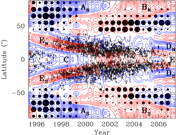
Figure 1.: Contours of constant residual rotation velocity, $\delta v_{\phi}=\delta\Omega r\cos\theta$, at $r=0.98R_{\odot}$ obtained from GONG data are shown as a function of time and latitude. The red contours show positive values while the blue contours show negative values. The contour spacing is 1 m s^-1 and the zero contour is not shown. Different bands of faster (e.g., $B_{N}$, $B_{S}$, $E$, $E_{N}$, $E_{S}$) and slower (e.g., $A_{N}$, $A_{S}$, $C$, $D_{N}$, $D_{S}$) than average rotation velocity are marked in the figure. The markings at low latitudes show the position of sunspots. The filled black circles at high latitudes represent the daily mean number of polar faculae averaged over a period of six months in $10^{\circ}$ latitude bins from $40^{\circ}$ to $90^{\circ}$. The area of the circles is proportional to the number of PFs.

2.2 Properties of Polar Faculae

2.2.1 Number Counts and Latitudinal Distribution

Soon after the polar-field reversal, which occurs after sunspot activity has reached its peak, polar faculae (abbreviated as PF) make their appearance in the latitude zones poleward of $40^{\circ}$ in both the hemispheres. They can be identified easily on the broad-band images as tiny bright features of sizes ranging from 3 – $10^{\prime\prime}$ with a contrast $I_{\rm PF}/I_{\rm photosphere}=1.03$ to 1.10 and on the K-line spectroheliograms as bright points located preferentially along the network boundaries i.e., along the boundaries of the supergranular cells (Makarov and Makarova 1996). The cyclically varying numbers of PF, which are $180^{\circ}$ out of phase with the sunspot number, over the entire solar disk are highly correlated with the polar magnetic-field strengths (Sheeley 1964, 1976, 1991). The total counts and the latitude distribution of PF determined for the period 1940 – 1985 by Makarov, Makarova, and Sivaraman (1989), Makarov and Sivaraman (1989), Makarov and Makarova (1996) have been extended to the present day by Makarov, Makarova, and Callebaut (in preparation). The procedure that was adopted for determining the total counts, as well as the latitude distribution of the PF, is described in Makarov and Makarova (1996) and may be summarised as follows: For every month, about 15 high-quality broad-band images were selected from the Kislovodsk Solar Station collections. The gaps in the data were filled in using the Ca ii K spectroheliograms of the Kodaikanal Observatory collections. The numbers of PF within the latitude zones starting from $40^{\circ}$ and reaching up to the poles were counted in steps of $10^{\circ}$ in order to derive their distribution. This was done plate by plate for the northern and southern hemispheres separately and from the counts so obtained for every month, the monthly and the six-monthly averages were worked out. We use the six-monthly mean values of PF in each of the $10^{\circ}$ bins for comparison with the zonal-flow pattern in Figure 1. These are represented by filled circles with area proportional to the six-monthly means plotted at the mean latitude positions of each of the $10^{\circ}$ bins.

The PFs appear first at latitude zones $\pm 40$ – $60^{\circ}$. The zones of appearance of the PF expand and reach almost to the poles filling the entire high-latitude regions during the sunspot minimum years. On average, about 900 PF emerge per day during this epoch. The zones of PF are seen to shrink progressively in extent during the rising phase of the then-current sunspot cycle until they finally disappear with the polar field reversal around the maximum phase (Figure 4 of Makarov and Sivaraman 1989). Sheeley and Warren (2006) used images and magnetograms from MDI to study PFs during the period 1996 – 2005 and showed that in each hemisphere there is a facula-free zone separating the old-cycle polar field from trailing-polarity flux that is migrating poleward from the sunspot belts. These facula-free zones coincide with the neutral lines of the axisymmetric component of photospheric magnetic field and their arrival at the poles in 2001 marks the reversal of the polar fields.

2.2.2 Magnetic Fields of Polar Faculae as the Source of Polar Fields

PFs have most commonly sizes in the range of 3 – $10^{\prime\prime}$ when they occur as individual structures or as bipoles, although a few of them appear at smaller sizes reaching down to $\approx 1^{\prime\prime}$. A few others showing a complex structure have sizes exceeding $10^{\prime\prime}$ and at times even as high as $30^{\prime\prime}$ (Makarov and Makarova 1996). In the magnetograms they appear in the form of flux knots either bright or dark depending on their magnetic polarity. Based on the polarimetric measurements by Homann, Kneer, and Makarov (1997), Makarov and Makarova (1998) estimate the magnetic flux per faculae to be $\approx 7\times 10^{19}$ Mx, while Varsik, Wilson, and Li (1999) estimate the flux to be $\approx 10^{19}$ Mx from calibrated low-resolution magnetograms. Thus the PFs possess a range of magnetic-field strengths from 150 to 1700 G depending on both their sizes and the amount of flux they carry, although PF with low field strengths appear to be more common.

The evolution of the integrated flux over the polar regions was traced by Lin, Varsik, and Zirin (1994) using high resolution magnetograms covering the period from early-1991 to mid-1993 that spans the maximum and declining phases of the sunspot cycle 22. According to them, during the solar-maximum phase, the polar regions are populated by magnetic elements of positive and negative polarity of almost equal numbers and of equal field strengths rendering the net fields at the poles close to zero. This presumably represents the polar-field reversal epoch. With the progress of the sunspot cycle towards the minimum, the elements of one polarity outnumber those of the opposite polarity in terms of the field strengths and numbers rendering the fields at the poles predominantly of one polarity. A subsequent study using more of such high-resolution magnetogram sequences during sunspot minimum phase by Varsik, Wilson, and Li (1999) confirms that knots of one polarity far exceed those of opposite polarity. It is this excess of one polarity flux elements over the other, itself varying cyclically (from + to $-$ and then to + and so on), that decides the polarity of the field at the poles of the Sun in any given cycle. It is the collective net field of the PF that a magnetograph operating at low resolution measures as the magnetic flux at the poles of the Sun during the sunspot minimum phase.

3 Results

3.1 Latitude Distribution of Sunspots and the Zonal Flow Pattern

We have shown in Figure 1 the latitudinal distribution of sunspots (the Butterfly pattern) extracted from the Greenwich sunspot data superposed on the plot of the zonal-velocity band pattern at $r=0.98R_{\odot}$. We find that the dense part of the distribution of spots lies over the zonal bands of the faster than average rotation rate ($E_{N}$ and $E_{S}$) while, the less dense part of the distribution spills over to the slow streams ($D_{N}$ and $D_{S}$). There is also a sprinkling of sunspots in the region C (the slow stream). These might possibly be very small spots or pores being the last vestiges of solar cycle 22 (1986 – 1996). Similar spatial coincidence between sunspot distribution and surface torsional oscillation pattern has been noted earlier by Snodgrass (1987).

3.2 PF Distribution and the High Latitude Zonal Flow Pattern

It is evident from Figure 1 that the polar-faculae distribution coincides well, both spatially and temporally, with the high-latitude zonal-band pattern ($A_{N}$ in the north and $A_{S}$ in the south hemispheres). Both the slow-stream bands $A_{N}$ and $A_{S}$ and the PF associated with them that have reached close to the respective poles disappear with the polar-field reversal in 2000.7. Two new zonal bands of fast streams ($B_{N}$ and $B_{S}$) that originated at $\pm 50^{\circ}$ latitudes about two years prior to the polar-field reversal, have now ascended poleward filling the latitude regions where $A_{N}$ and $A_{S}$ were present before the polar-field reversal. The PF of the new cycle (2002 – 2006) that appeared soon after the polar-field reversal coinciding with the new fast streams $B_{N}$ and $B_{S}$ have also migrated polewards synchronously with the fast streams. The polar-field reversal in 2000.7 that marks the end of one PF cycle and the beginning of the next one in both hemispheres is also the epoch that marks the end of the slower-than-average rotation-rate zonal bands at the poles ($A_{N}$ and $A_{S}$) and the ascendancy of the new faster than average rotation rate zonal bands ($B_{N}$ and $B_{S}$) to their positions. Thus the distribution of polar faculae that provides the magnetic field at the poles shows a distribution in latitude and time similar to the zonal flow pattern of the sub-surface layers at $r=0.98R_{\odot}$ at high latitudes. Although, we have used the zonal-flow pattern at $r=0.98R_{\odot}$ for establishing the spatial and temporal coincidence with the PF, similar correspondence should hold for all sub-surface layers lying above $r=0.95R_{\odot}$. Below $r=0.90R_{\odot}$ the zonal-flow pattern appears to be smeared out and the phase also changes at low latitudes. Thus at $r=0.8R_{\odot}$ the fast and slow streams can hardly be recognised at the high latitudes (Antia and Basu 2001, Figure 4; Basu and Antia 2006, Figure 1). At any rate it appears that the correspondence between zonal flow pattern and the PF seems to be confined to the layers above $r=0.95R_{\odot}$.

4 Discussion and Conclusions

We have derived the residual rotation rates by subtracting the time-averaged rotation rate from that at each epoch from helioseismic data from the GONG project for a full solar cycle (1996 – 2007) at $r=0.98R_{\odot}$ in the solar interior. These show a set of zonal velocity bands moving with faster- and slower-than-average rotation rate. The zonal velocity bands have two components per hemisphere (Figure 1) (a) the high-latitude component of alternating slow (blue contours) and fast (red contours) streams (above $\approx 50^{\circ}$) that move poleward ($A_{N}$ or $A_{S}$ and $B_{N}$ or $B_{S}$), (b) the low-latitude component of fast ($E_{N}$ or $E_{S}$) and slow ($D_{N}$ or $D_{S}$) streams in the sunspot latitudes that move towards the Equator. $E_{N}$ and $E_{S}$ later merge to form a single fast stream $E$. From the earlier studies (Vorontsov et al. 2002; Basu and Antia 2003) it is known that the zonal flows in the high-latitude as well as in the sunspot-latitude belts persist throughout much of the convection zone and are quite stable. The $\approx 50^{\circ}$ latitude in the two hemispheres seems to be the boundary that separates the high latitude streams from the low latitude streams. Interestingly, this is also the latitude region where the rotation rate residual is close to zero throughout almost the entire convection zone (Vorontsov et al. 2002; Basu and Antia 2006).

We have established that (a) polar faculae and the zonal-flow bands in the region above $\pm 40$ – $50^{\circ}$ latitudes have very similar distribution in the spatial and temporal domains, irrespective of whether the zonal velocity band is a fast stream or a slow stream (Figure 1). The switch from fast to slow happens around sunspot minimum (around 1996) when there is no reversal in polarity of the polar magnetic field, while the switch from slow to fast occurs around the sunspot maximum which coincides with field polarity reversal at the poles around 2000.7. Thus there is one pair of streams (one fast and one slow) during the period of two successive polar-field reversals and both components of the pair are associated with polar fields of the same polarity either positive or negative as the case might be. (b) In the sunspot latitudes, the butterfly pattern coincides with the fast streams ($E_{N}$, $E_{S}$ or $E$) although part of the sunspot distribution spills over to the slow streams ($D_{N}$ and $D_{S}$) too (Figure 1). Of course, our study is restricted to one solar cycle for which the seismic data is available and this association needs to be confirmed in subsequent cycles.

We have also established that there is a striking similarity in spatial and temporal organisation between the zonal-flow streams in the interior and the surface magnetic fields. This would imply a close coupling between the periodic components of flows in the interior and the surface magnetic-field structures which are visible manifestations of the cyclic magnetic activity. This close similarity raises interesting possibilities about their connection links (cf., Snodgrass 1987). Clearly, the velocity changes present in the zonal flow alone are intrinsically too weak to drive the global solar-activity cycle. It is, therefore, possible that both the zonal-flow pattern and the overall solar magnetic activity are manifestations of a common coherently-driven global mechanism that remains to be identified and properly understood. There could be other possibilities: two mechanisms operating on disparate scales at two different depths in the convection zone could conceivably result in mutually-coherent velocity and magnetic field patterns. It is commonly accepted that the shear zone below the base of the convection zone is the seat of the dynamo that amplifies and produces the strong magnetic field that gives rise to sunspots. Likewise, there is an amplification of the magnetic field by the shear in the sub-surface layers between $r=0.98R_{\odot}$ and $0.95R_{\odot}$ that could produce weaker fields like those in the polar faculae (Dikpati et al. 2002). The possible role of the near-surface shear layer in small scale amplification of magnetic field has been envisaged earlier by Gilman (2000). More sophisticated theoretical models supported by simulations to explore the mechanisms that can generate and sustain the zonal-band systems in the interior and also organise the magnetic fields in a mutually coherent way are clearly needed. It is gratifying to note that initial efforts in this direction have already produced migrating patterns (e.g., Covas et al. 2000; Covas, Tavakol, and Moss 2001; Covas, Moss, and Tavakol 2004; Lanza 2007). It would equally be important to explore the role of the subsurface shear region in small-scale amplification of magnetic fields and to explain the intimate relationship between the family of zonal-band system and the distribution of magnetic flux elements.

The helioseismic data from GONG and MDI accumulated over the past solar cycle 23 enabled Antia, Chitre, and Gough (2008) to study temporal variations in the solar rotational kinetic-energy. It was demonstrated that at high latitudes ($>45^{\circ}$) variation in the kinetic energy through the convection zone is correlated with the solar activity, while in the equatorial latitudes ($<45^{\circ}$) it is anticorrelated except for the upper 10% of the solar radius where both are in phase. The amplitude of temporal variation of the rotational kinetic-energy integrated over the entire convection zone turns out to be $\approx 3\times 10^{38}$ ergs implying a rate of variation of about $5\times 10^{30}$ ergs s^-1 over the solar cycle. From energy conservation it is expected that the torsional kinetic-energy variation is comparable with that in the magnetic energy but with opposite phase. It thus seems that the temporal variation in rotational kinetic energy in the convection zone is related to the solar cycle with its tantalising similarity with the magnetic activity cycle.

Acknowledgements

This work utilises data obtained by the Global Oscillation Network Group (GONG) project, managed by the National Solar Observatory, which is operated by AURA, Inc. under a cooperative agreement with the National Science Foundation. The data were acquired by instruments operated by the Big Bear Solar Observatory, High Altitude Observatory, Learmonth Solar Observatory, Udaipur Solar Observatory, Instituto de Astrofisico de Canarias, and Cerro Tololo Inter-American Observatory. We thank Baba Varghese for his valuable help in formulating the Figure. S.M.C. thanks the Indian National Science Academy for support under the INSA Honorary Scientist programme.

References

- [Antia and Basu(2000)] Antia, H.M., Basu, S.: 2000, Astrophys. J. 541, 442.
- [Antia and Basu(2001)] Antia, H.M., Basu, S.: 2001, Astrophys. J. 559, L67.
- [Antia, Basu, and Chitre(1998)] Antia, H.M., Basu, S., Chitre, S.M.: 1998, Mon. Not. Roy. Astron. Soc. 298, 543.
- [Antia, Chitre, and Gough(2008)] Antia, H.M., Chitre, S.M., Gough, D.O.: 2008, Astron. Astrophys. 477, 657.
- [Basu and Antia(2003)] Basu, S., Antia, H.M.: 2003, Astrophys. J. 585, 553.
- [Basu and Antia(2006)] Basu, S., Antia, H.M.: 2006, In: Fletcher, K., Thompson, M.J. (eds.) SOHO 18/GONG 2006/HELAS I, Beyond the spherical Sun, SP-624, ESA Publ. Div., Noordwijk, 128.
- [Covas et al.(2004)] Covas, E., Moss, D., Tavakol, R.: 2004, Astron. Astrophys. 416, 775.
- [Covas, Tavakol, and Moss(2001)] Covas, E., Tavakol, R., Moss D.: 2001, Astron. Astrophys. 371, 718.
- [Covas, Moss, and Tavakol(2000)] Covas, E., Tavakol, R., Moss, D., Tworkowski, A.: 2000, Astron. Astrophys. 360, L21.
- [Dikpati et al.(2002)] Dikpati, M., Corbard, T., Thompson, M.J., Gilman, P.A.: 2002, Astrophys. J. 575, L 41.
- [Gilman(2000)] Gilman, P.A.: 2000, Solar Phys. 192, 27.
- [Hill et al.(1996)] Hill, F., et al.: 1996, Science 272, 1292.
- [Homann, Kneer, Makarov(1997)] Homann, T., Kneer, F., Makarov, V.I.: 1997, Solar Phys. 175, 81.
- [Howard and LaBonte(1980)] Howard, R.F., LaBonte, B.J.: 1980, Astrophys. J. 239, L33.
- [Howe et al.(2000)] Howe, R., Christensen-Dalsgaard, J., Hill, F., Komm, R.W., Larsen, R.M., Schou, J., Thomson, M.J., Toomre, J.: 2000, Astrophys. J. 533, L163.
- [Howe et al.(2006)] Howe, R., Rempel, M., Christensen-Dalsgaard, J., Hill, F., Komm, R.W., Larsen, R.M., Schou, J., Thompson, M.J.: 2006, Astrophys. J. 649, 1155.
- [Lanza(2007)] Lanza, A.F.: 2007, Astron. Astrophys. 471, 1011.
- [Lin, Varsik, and Zirin(1994)] Lin, H., Varsik, J., Zirin, H.: 1994, Solar Phys. 155, 243.
- [Makarov and Makarova(1996)] Makarov, V.I., Makarova, V.V.: 1996, Solar Phys. 163, 267.
- [Makarov and Makarova(1998)] Makarov, V.I., Makarova, V.V.: 1998, In: Balasubramaniam, K.S., Harvey, J.W., Rabin, D.M. (eds.) Synoptic Solar Physics, ASP Conf. Ser. 140, Astron. Soc. Pac., San Francisco, 347.
- [Makarov and Sivaraman(1989)] Makarov, V.I., Sivaraman, K.R.: 1989, Solar Phys. 123, 367.
- [Makarov, Makarova, and Sivaraman(1989)] Makarov, V.I., Makarova, V.V., Sivaraman, K.R.: 1989, Solar Phys. 119, 45.
- [Schou(1999)] Schou, J.: 1999, Astrophys. J. 523, L181.
- [Sheeley(1964)] Sheeley, N.R., Jr.: 1964, Astrophys. J. 140, 731.
- [Sheeley(1976)] Sheeley, N.R., Jr.: 1976, J. Geophys. Res. 81, 3462.
- [Sheeley(1991)] Sheeley, N.R., Jr.: 1991, Astrophys. J. 374, 386.
- [Sheeley and Warren(2006)] Sheeley, N.R., Jr., Warren, H.P.: 2006, Astrophys. J. 641 611.
- [Snodgrass and Howard(1985)] Snodgrass, H.B., Howard, R.F.: 1985, Science, 228, 945.
- [Snodgrass(1987)] Snodgrass, H.B.: 1987, Solar Phys. 110, 35.
- [Snodgrass(1992)] Snodgrass, H.B.: 1992, In: Harvey, K.L. (ed.) Solar Cycle Workshop ASP Conf. Ser. 27, Astron. Soc. Pac., San Francisco, 205.
- [Ulrich(2001)] Ulrich, R.K.: 2001, Astrophys. J. 560, 466.
- [Ulrich et al.(1988)] Ulrich, R.K., Boyden, J.E., Webster, L., Snodgrass, H.B., Padilla, S.P., Gilman, P., Shieber, T.: 1988, Solar Phys. 117, 291.
- [Varsik, Wilson, and Li(1999)] Varsik, J.R., Wilson, P.R., Li, Y.: 1999, Solar Phys. 184, 223.
- [Vorontsov et al.(2002)] Vorontsov, S.V., Christensen-Dalsgaard, J., Schou, J., Strakhov, V.N., Thomson, M.J.: 2002, Science 296, 101.