PHASE-TRANSIENT HIERARCHICAL TURBULENCE AS AN ENERGY CORRELATION
GENERATOR OF BLAZAR LIGHT CURVES

Abstract

Hierarchical turbulent structure constituting a jet is considered to reproduce energy-dependent variability in blazars, particularly, the correlation between X- and gamma-ray light curves measured in the TeV blazar Markarian 421. The scale-invariant filaments are featured by the ordered magnetic fields that involve hydromagnetic fluctuations serving as electron scatterers for diffusive shock acceleration, and the spatial size scales are identified with the local maximum electron energies, which are reflected in the synchrotron spectral energy distribution (SED) above the near-infrared/optical break. The structural transition of filaments is found to be responsible for the observed change of spectral hysteresis.

1. INTRODUCTION

A noticeable feature associated with blazars is that the updated shortest variability timescale reaches a few minutes (e.g., Mrk 421: Cui, 2004; Błażejowski et al., 2005), not likely to be reconciled with the light-crossing time at the black hole horizon. One possible explanation for this fact is that small-scale structure does exist in the parsec-scale jet anchored in the galactic core (Honda & Honda, 2004). Indeed, in the plausible circumstance that the successive impingement of plasma blobs (ejected from the core) into the jet bulk engenders collisionless shocks, electromagnetic current filamentation (characterized by the skin depth) could be prominent (Medvedev & Loeb, 1999). It is known that the merging of smaller filaments leads eventually to accumulation of magnetic energy in larger scales (Honda et al., 2000a; Silva et al., 2003).

Reflecting the self-similar (power law) characteristic in the inertially cascading range, the local magnetic intensity of the self-organized filaments will obey $|{\bf B}|\sim B_{m}(\lambda/d)^{(\beta-1)/2}$, where $\lambda$ and $d$ reflect the transverse size scale of a filament and the maximum, respectively, $B_{m}\equiv|{\bf B}|_{\lambda=d}$, and $\beta$ $(>1)$ corresponds to the filamentary turbulent spectral index. The value of $d$ is limited by the transverse size of jet (or blob size; $D$). Then, it is reasonable to consider that in fluid timescales, the well-developed coherent fields are sure to actually meet hydromagnetic disturbance independent of the filamentation; that is, the turbulent hierarchy is established (see Fig. 1). The spectral index of the superposed fluctuations [denoted as $\beta^{\prime}$ $(>1)$] could be different from $\beta$, and the correlation length scale is presumably limited by $\sim\lambda$.

At this site, the electrons bound to the local mean fields suffer scattering by the fluctuations, to be diffusively accelerated by the collisionless shocks (see Honda & Honda, 2007). When the acceleration and cooling efficiency depend on the spatial size scales, the local maximum energies of accelerated electrons will be identified by $\lambda$ (§ 2), to be reflected in the synchrotron SED extending to the X-ray region. More interestingly, the spatially inhomogeneous property of particle energetics is expected to cause the energy-dependent variability of broadband SEDs. Here the naive question arises whether or not this idea is responsible for the observed elusive patterns of energy correlation of light curves (e.g., Takahashi et al., 1996; Fossati et al., 2000a, b; Błażejowski et al., 2005): this is the original motivation of the current work.

In the present simplistic model, light travel time effects would still prevent the detection of variability signatures on timescales shorter than $D/(c\delta_{z})$, where $\delta_{z}=\delta/(1+z)$, and $\delta$, $z$, and $c$ are the beaming factor of the jet, redshift, and speed of light, respectively. However, if a filamented piece is isolated, having loose causal relation with the dynamics of a bulk region serving as a dominant emitter, an intrinsic rapid variability involved in the subsystem would be viable. Namely, it is inferred that the shorter timescale is at least potentially realized, and observable, unless energetic emissions from such a compact domain are crucially degraded by synchrotron self-absorption and/or $\gamma\gamma$ absorption (e.g., Aharonian, 2004). As is, the basic notion of the present model seems to provide a vital clue to settle the debate as to the causality problem incidental to observed rapid variabilities.

In this Letter, I demonstrate that the hierarchical system incorporated with the synchrotron self-Compton (SSC) mechanism accurately generates the time lag of gamma-ray flaring activity behind the X-ray, confirmed in the high-frequency-peaked BL Lac object Mrk 421 (Błażejowski et al., 2005). We address that in general, both lag and lead can appear in X-ray interband correlations, accompanying the structural transition. The major transition history is argued in light of the observed spectral hysteresis patterns. We also work out $(B_{m},d)$, to provide the constraint on the field strength and $D$ that should be compared with those of previous models.

2. AN IMPROVED EMITTER MODEL WITH
HIERARCHICAL STRUCTURE

We consider a circumstance in which relativistic shocks propagate through a relativistic jet with the Lorentz factor $\Gamma$, such that the shock viewed upstream (jet frame) is weakly to mildly relativistic. Note the relation of $\delta\sim\Gamma$. The overall geometry and relative size scales of the aforementioned hierarchy are sketched in Figure 1. Provided that the gyrating electrons trapped in the filament (with the size $\lambda$) are resonantly scattered by the magnetic fluctuations, the mean acceleration time upstream is approximately given by $\tau_{\rm acc}\simeq(3\eta r_{\rm g}/c)[r/(r-1)]$, where $\eta=(3/2b)(\lambda/2r_{\rm g})^{\beta^{\prime}-1}$, $b$ is the energy density ratio of fluctuating/local mean magnetic fields (assumed to be $b\ll 1$), $r_{\rm g}(\gamma,|{\bf B}|)$ is the electron gyroradius ($\gamma$ being the Lorentz factor), and $r$ is the shock compression ratio. In the regime in which flares saturate, $\tau_{\rm acc}$ will be comparable to synchrotron cooling time $\tau_{\rm syn}(\gamma,|{\bf B}|^{2})$. Balancing these timescales gives the (local) maximum $\gamma$ of an accelerated electron, described as $\gamma^{\ast}(\lambda)=\{g_{0}^{-(\beta^{\prime}-1)}g_{1}\left(\lambda/d\right)^{-[(\beta+1)\beta^{\prime}-2]/2}\}^{1/(3-\beta^{\prime})}$, where $g_{0}=eB_{m}d/(2m_{e}c^{2})$, $g_{1}=8\pi^{2}\xi m_{e}^{2}c^{4}/(e^{3}B_{m})$, $\xi=b(r-1)/r$, and the other notations are standard. At $\gamma=\gamma^{\ast}$, the electron energy distribution of the power-law form $n(\gamma)d\gamma=\kappa\gamma^{-p}d\gamma$ is truncated.

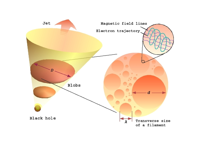
Figure 1.— Schematic of the beamed jet including the emitting blobs and top view of the transverse cut of a blob region (with the diameter $D$). A number of circle-like ”bubbles” symbolically represent the transverse section of scale-invariant filaments (with size $\lambda$, whose maximum is $d$). Note that $d$ is limited by $D$ (for the values, see § 4). The magnified view of a small sample domain illustrates the fluctuating magnetic field that scatters gyrating electrons bound to the local mean field.

For simplicity, $\kappa$ and $\xi$ are assumed to be spatially constant at the moment. Then, for $\beta^{\prime}<3$ (see § 3.1), $\gamma^{\ast}$ decreases as $\lambda$ increases (reflecting likely prolonged $\tau_{\rm acc}$ and shortened $\tau_{\rm syn}$), to take a minimum value at $\lambda=d$, where the synchrotron flux density makes, up to the frequency of $(3/4\pi)(\delta_{z}\gamma^{\ast}|_{\lambda=d}^{2}eB_{m}/m_{e}c)(\equiv\nu_{b})$, a dominant contribution to the $F_{\nu}$ spectrum (owing to the maximum magnetic intensity at the outer scale). As $\lambda$ decreases, the flux density tends to decrease, extending the spectral tail (due to the $\gamma^{\ast}$ increase). Apparently, this property has the $F_{\nu}$ spectrum steepening above $\nu_{b}$, whereas below $\nu_{b}$ the spectrum retains $F_{\nu}\propto\nu^{-(p-1)/2}$. The frequency $\nu_{b}$ characterizing the spectral break can be expressed as $\nu_{b}=7.5\times 10^{14}\delta_{50}B_{m,10}^{-3/2}\xi_{-4}^{3/2}d_{16}^{-1}~{}{\rm Hz}$ (for $\beta^{\prime}=5/3$; see § 3.1), where $\delta_{50}=\delta_{z}/50$, $B_{m,10}=B_{m}/10\,{\rm G}$, $d_{16}=d/10^{16}\,{\rm cm}$, $\xi_{-4}=\xi/10^{-4}$, and $\xi=b(r-1)/r$.

The increase of $\gamma^{\ast}$ in smaller $\lambda$ is limited at a critical $\lambda_{c}$, below which escape loss dominates the radiative loss: the equation for the spatial limit, $r_{g}(\gamma^{\ast})\sim\lambda/2$, yields $\lambda_{c}/d\sim(g_{0}^{-2}g_{1})^{2/(3\beta+1)}$. By using this expression, one can evaluate the achievable maximum $\gamma^{\ast}$ value as $\gamma^{\ast}|_{\lambda=\lambda_{c}}=g_{0}(\lambda_{c}/d)^{(\beta+1)/2}$, for which the corresponding synchrotron cutoff frequency is $\nu_{c}=\delta_{z}\nu_{0}g_{0}^{2}(\lambda_{c}/d)^{(3\beta+1)/2}=\delta_{z}\nu_{0}g_{1}$, where $\nu_{0}=(3/4\pi)(eB_{m}/m_{e}c)$. Also, by combining $\lambda_{c}\propto\nu_{c}^{2/(3\beta+1)}$ with $F_{\nu_{c}}\propto|{\bf B}(\lambda_{c})|^{(p+1)/2}\nu_{c}^{-(p-1)/2}$, we read $\ln(\nu F_{\nu})_{c}/\ln\nu_{c}\propto[(5-p)\beta-(p-1)]/(3\beta+1)$ at $\nu\sim\nu_{c}$. More speculatively, this scaling might be reflected in $\ln(\nu F_{\nu})_{p}/\ln\nu_{p}$ for measured synchrotron flux peaks.

3. PROPERTIES OF ENERGY-DEPENDENT SPECTRAL
VARIABILITY AND HYSTERESIS

3.1. X-Ray Interband Correlation

In this context, we derive the $\nu$-dependence of the flaring activity timescale (denoted as $\tau$). In $\nu_{b}<\nu<\nu_{c}$, which typically covers the X-ray band, we have $\gamma^{\ast}=[(4\pi/3)(\nu/\delta_{z})(m_{e}c/e|{\bf B}|)]^{1/2}$, which is written as $\gamma^{\ast}(\lambda,\nu)=(\nu/\delta_{z}\nu_{0})^{1/2}(\lambda/d)^{-(\beta-1)/4}$. Utilizing this, the expression of $\tau_{\rm syn}(\gamma^{\ast},|{\bf B}|^{2})$ is recast into $\tau_{\rm syn}(\lambda,\nu)(=\tau_{\rm acc}\sim\delta_{z}\tau)=(\tau_{0}/\delta_{z})(\delta_{z}\nu_{0}/\nu)^{1/2}(\lambda/d)^{-3(\beta-1)/4}$, where $\tau_{0}=36\pi^{2}m_{e}^{3}c^{5}/(e^{4}B_{m}^{2})$. The relation of $\lambda$ to $\nu$ can be derived from the equality of $\gamma^{\ast}(\lambda,\nu)=\gamma^{\ast}(\lambda)$, such that $\lambda(\nu)/d=\{g_{0}^{-1}g_{1}^{1/(\beta^{\prime}-1)}(\delta_{z}\nu_{0}/\nu)^{(3-\beta^{\prime})/[2(\beta^{\prime}-1)]}\}^{4/(3\beta+1)}$. Substituting this into $\tau(\lambda,\nu)$, we arrive at the result $\tau(\nu)\sim(\tau_{0}/\delta_{z})(\nu/\delta_{z}\nu_{0})^{(\sigma-1)/2}(g_{0}^{\beta^{\prime}-1}g_{1}^{-1})^{\sigma/(3-\beta^{\prime})}$, where $\sigma(\beta,\beta^{\prime})=3(\beta-1)(3-\beta^{\prime})/[(3\beta+1)(\beta^{\prime}-1)]$; that is,

$$\tau\propto\nu^{-(1/2)(1-\sigma)}.$$ (1)

Note that $\sigma=0$ (for $\beta=1$) leads to $\tau\propto\nu^{-1/2}$, formally recovering the scaling for a homogeneous model. Significantly, the states of $\sigma<1$ and $>1$ imply the appearance of the modes for which the X-ray activity in a lower $\nu$ lags that in a higher $\nu$ (”soft lag”; Takahashi et al., 1996; Rebillot et al., 2006) and vice versa (”hard lag”; Fossati et al., 2000a), respectively, and $\sigma=1$ is the tight-correlation mode (Sembay et al., 2002). The mode flipping comes about through competing $\lambda$-dependence of cooling and acceleration efficiency. In particular, the soft lag appears if

$$\beta<\beta_{c}=(4-\beta^{\prime})/[3(2-\beta^{\prime})].$$ (2)

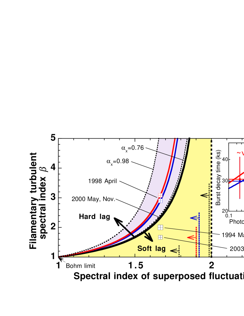
Figure 2.— Phase diagram of the hierarchical turbulence. The function $\beta_{c}(\beta^{\prime})$ (eq. [2]; thick solid curve) divides the $(\beta,\beta^{\prime})$-plane into the two domains that allow soft-lag ($\beta<\beta_{c}$; yellow) and hard-lag ($\beta>\beta_{c}$) in the X-ray band. The possible phases $\Phi_{2}$ $(2,5/3)$ and $\Phi_{5/3}$ $(5/3,5/3)$ (large and small marks, respectively) involve soft-lag, as consistent with the correlations measured in the labeled epochs. The inset shows the power-law fit to two available $\tau$-$\nu$ data on 1998 April 21 (for detailed data reduction, see Fossati et al., 2000a), giving the indices of $s=0.11$ and $0.087$ (corresponding colors), which determine $\beta(\beta^{\prime};s)$ (colored curves) for $\beta^{\prime}<(s+2)/(s+1)$ (colored arrows). The characteristic curves lie in a domain (purple; $\beta^{\prime}$-range is indicated by thin solid arrows) restricted by the measured X-ray spectral indices (and $p=1.6$; Fossati et al., 2000b), and give $\beta=3.1$ and $2.9$ (colored marks) at $\beta^{\prime}=5/3$. For further explanation, see the text.

The critical function $\beta_{c}(\beta^{\prime})$ is, for the key range of $(1<)\beta^{\prime}<2$, plotted in Figure 2. Note that for the special $\beta^{\prime}=2$ case, $\sigma[=3(\beta-1)/(3\beta+1)]<1$ is always satisfied, and $\beta^{\prime}>2$ ensures $\beta>\beta_{c}$ (because of $\beta_{c}<1$): $\beta^{\prime}=2$ and $>2$ lead to soft and hard lag, respectively, irrespective of the $\beta$ value. While the index $\beta$ is expected to be variable (reflecting the long-term structural evolution of filaments; see § 3.3 for details), $\beta^{\prime}$ would be a constant since a mechanism of superimposed magnetic fluctuations (§ 1) perhaps has universality. One can exclude $\beta^{\prime}>2$, which yields by no means soft lag, which is at odds with the observational facts, whereupon we can take the modified upper bound (indicated in Fig. 2, arrows) into account. With these ingredients, I conjecture the preferential appearance of $\beta^{\prime}=5/3$ (the Kolmogorov-type turbulence), for which $\beta_{c}=7/3$. As for $\beta$, it appears that for $\beta=2$ (Montgomery & Liu, 1979) and $5/3$ (and given $\beta^{\prime}=5/3$), the model synchrotron spectra of $\nu F_{\nu}\propto\nu^{0.32}$ and $\nu^{0.40}$ (in $\nu_{b}<\nu<\nu_{p}$; $\nu F_{\nu}\propto\nu^{0.69}$ in $\nu<\nu_{b}$) provide a reasonable fit to the measured ones (at flares) in the mid state (2002–2003) and high state (2004–2005), respectively, of Mrk 421, suggesting $\nu_{b}\sim 2\times 10^{14}\,{\rm Hz}$ (not shown in figure), as compatible with smaller variability in the $\nu$-range below R band (Błażejowski et al., 2005). Below, we refer to these possible phases $(\beta,\beta^{\prime})=(2,5/3)$ and $(5/3,5/3)$, which satisfy equation (2), as ”$\Phi_{2}$” and ”$\Phi_{5/3}$”, respectively. Also, we compare with the detailed data of burst decay time (in 1998; Fossati et al., 2000a). The guideline is given in Figure 2: use is made of the translation of the measured timescale $\propto\nu^{s}$ to $\beta=[4-\beta^{\prime}+s(\beta^{\prime}-1)]/\{3[2-\beta^{\prime}-s(\beta^{\prime}-1)]\}$. This characteristic curve for $s\simeq 0.1$ indicates $\beta\simeq 3$ at $\beta^{\prime}=5/3$, and $\beta>\beta_{c}$, as consistent with the measured hard lag. For these $\beta=5/3$, $2$, and $3$, we anticipate $(\nu F_{\nu})_{p}\propto\nu_{p}^{0.8}$, $\nu_{p}^{0.9}$, and $\nu_{p}$ (for $p\simeq 1.6$; e.g., Macomb et al., 1995), amenable to the full X-ray data analysis of Mrk 421 flares (Tramacere et al., 2007).

Let us now estimate the time lag of a soft energy band $\epsilon_{\rm L}$($>h\nu_{b}$; $h$ is the Planck constant) behind a hard band $\epsilon_{\rm H}(<h\nu_{c})$ by $\Delta\tau=\tau(\epsilon_{\rm L})-\tau(\epsilon_{\rm H})$. Here it is instructive to note the relation of $(\lambda_{c}<)$ $\lambda(\epsilon_{\rm H})<\lambda(\epsilon_{\rm L})$ $(<d)$. Using the expression of $\nu_{b}$ (eliminating $\xi^{3/2}d^{-1}$), we obtain

$$\Delta\tau=1.8\,\delta_{50}^{-1/2}B_{m,10}^{-3/2}\nu_{b,14}^{-3/7}\epsilon_{{\rm L},1}^{-1/14}\eta_{-1}~{}{\rm hr}$$ (3)

for the structural phase $\Phi_{2}$, where $\nu_{b,14}=\nu_{b}/10^{14}\,{\rm Hz}$, $\eta_{-1}=[1-(\epsilon_{\rm L}/\epsilon_{\rm H})^{1/14}]/10^{-1}$, and $\epsilon_{{\rm L},1}=\epsilon_{\rm L}/1\,{\rm keV}$. Concerning the validity, it has been checked that, e.g., for a soft-lag episode (in 1994 May; Takahashi et al., 1996), the measured time lag plotted against $\epsilon_{\rm L}$ could be more naturally fitted by the function (3) of $\Delta\tau(\epsilon_{\rm L},\epsilon_{\rm H})$ (given $\epsilon_{\rm H}\simeq 4-5\,{\rm keV}$ for ASCA), rather than the function of $\sim\epsilon_{\rm L}^{-1/2}[1-(\epsilon_{\rm L}/\epsilon_{\rm H})^{1/2}]$ for the homogeneous ($\sigma=0$) model.

3.2. X/Gamma-Ray Cross-Band Correlation

The interband correlation property is reflected in the cross-band correlation between X- and gamma-rays, provided the SSC mechanism as a dominant gamma-ray emitter (e.g., Maraschi et al., 1992; Dermer & Schlickeiser, 1993). Along the heuristic (time independent) manner, we suppose $\gamma\sim\gamma^{\ast}$ for scattering electrons, and examine the correlation between an X-ray band $\epsilon_{\rm x}$ (compared to $\epsilon_{\rm H}$) and gamma-ray band $\epsilon_{\gamma}$ susceptible to the inverse Comptonization of low-energy synchrotron photons (with $\epsilon_{\rm L}$). Here we focus on the feasible, Thomson regime of $(\epsilon_{\rm L}/\delta_{z})\gamma^{\ast}<m_{e}c^{2}$; note that using the expression of $\gamma^{\ast}[\lambda(\epsilon_{\rm L})]$ (§ 3.1), this range can be written as $\epsilon_{\rm L}<\delta_{50}[B_{m,10}^{2}(\xi_{-4}^{3/2}d_{16}^{-1})]^{2/23}~{}{\rm keV}$ (for $\Phi_{2}$). The Lorentz factor of the electrons that execute the boost of $\epsilon_{\gamma}/\epsilon_{\rm L}=(\gamma^{\ast})^{2}$ is denoted as $\gamma_{s}^{\ast}=(\epsilon_{\gamma}/\delta_{z}h\nu_{0})^{1/4}[\lambda(\epsilon_{\rm L})/d]^{-(\beta-1)/8}$. Then, simply estimating $\Delta\tau_{\gamma{\rm x}}=\tau[\epsilon_{\gamma}/(\gamma_{s}^{\ast})^{2}]-\tau(\epsilon_{\rm x})$ ($>0$, for $\beta<\beta_{c}$) would be adequate for the present purpose. For convenience, one may eliminate $\epsilon_{\rm L}$ from $\gamma_{s}^{\ast}$ [transform $\lambda(\epsilon_{\rm L})$ into $\lambda(\epsilon_{\gamma})$], and adopt the positive soft-lag representation of $\Delta\tau_{{\rm x}\gamma}(=-\Delta\tau_{\gamma{\rm x}})$, so that the negative sign indicates gamma-ray lag. Again using $\nu_{b}$, we find for $\Phi_{2}$

$$\Delta\tau_{{\rm x}\gamma}=-1.7\,\delta_{50}^{-5/32}B_{m,10}^{-7/8}\nu_{b,14}^{-7/16}\epsilon_{\gamma,1}^{-1/32}\eta_{\gamma{\rm x},-1}~{}{\rm days},$$ (4)

where $\eta_{\gamma{\rm x},-1}=\{1-0.79\epsilon_{{\rm x},25}^{-1/14}[(\epsilon_{\gamma,1}\delta_{50}B_{m,10})^{1/2}\times$ $\nu_{b,14}^{1/7}]^{1/16}\}/10^{-1}$, $\epsilon_{\gamma,1}=\epsilon_{\gamma}/1\,{\rm TeV}$, and $\epsilon_{{\rm x},25}=\epsilon_{\rm x}/25\,{\rm keV}$. The simultaneous equations (3) and (4) contain the solutions $(\delta,B_{m})$, for given observable quantities $\nu_{b}$ and $(\Delta\tau,\Delta\tau_{{\rm x}\gamma})$, as well as $(\epsilon_{\rm L},\epsilon_{\rm H};\epsilon_{\rm x},\epsilon_{\gamma})$ inherent in detectors.

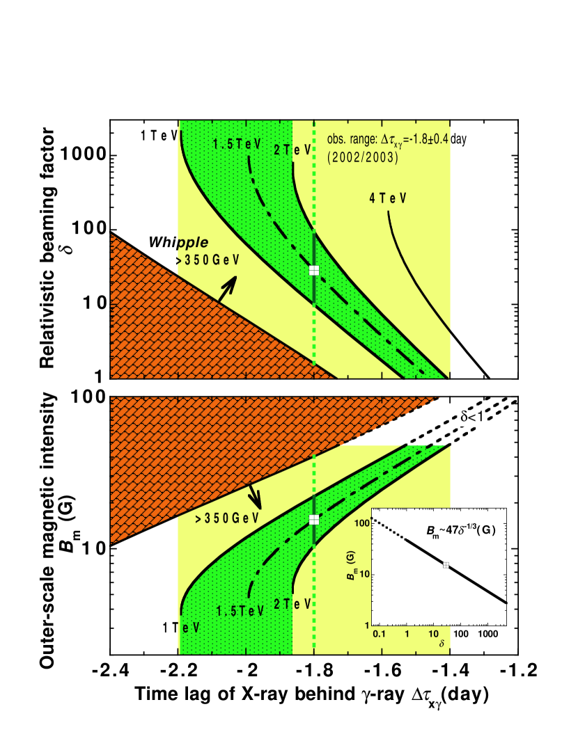
Figure 3.— Beaming factor $\delta$ (top) and maximum field strength $B_{m}$ (bottom) vs. the time lag of X-ray behind gamma-ray $\Delta\tau_{{\rm x}\gamma}$ ($<0$ means gamma-ray lag) for a given gamma-ray band $\epsilon_{\gamma}$ (labeled) as a parameter. The horizontal axes are common in the panels. The correlation is taken between $\epsilon_{\rm x}=25\,{\rm keV}$ and $\epsilon_{\gamma}\geq 350\,{\rm GeV}$ compared to an RXTE band and coverage of the Whipple 10 m telescope (brick-like shaded area indicates the prohibited domains), respectively. The hatched bands (green) indicate the allowed domains for $\epsilon_{\gamma}=1-2\,{\rm TeV}$ and $\delta>1$, which cover the measured $\Delta\tau_{{\rm x}\gamma}=-1.8\pm 0.4\,{\rm days}$ (yellow) and give $\delta=10-92$ and $B_{m}=10-22\,{\rm G}$ at $\Delta\tau_{{\rm x}\gamma}=-1.8\,{\rm days}$ (deep green bars; say, $\delta=29$ and $B_{m}=16\,{\rm G}$ [marks] for $\epsilon_{\gamma}=1.5\,{\rm TeV}$ [dot-dashed curves]). The inset in the bottom panel shows the $B_{m}$-$\delta$ relation independent of $\epsilon_{\gamma}$.

In Figure 3 (top) for $\nu_{b,14}=2$, $\Delta\tau=1\,{\rm hr}$, and $(\epsilon_{{\rm L},1},\epsilon_{\rm L}/\epsilon_{\rm H};\epsilon_{{\rm x},25})=(1,0.2;1)$, compared to Mrk 421 ($z=0.031$) measurements (Takahashi et al., 1996; Błażejowski et al., 2005), the self-consistent numerical solution $\delta$ is plotted against $\Delta\tau_{{\rm x}\gamma}$, given $\epsilon_{\gamma}$ that covers a gamma-ray band associated with the Whipple observation (Catanese & Weekes, 1999). For the allowed domain of $\delta>1$ (Piner et al., 1999), a typical TeV range of $\epsilon_{\gamma,1}\simeq 1-2$ (susceptible to the significant variation in the mid state) is found to a priori restrict the domain of the observable $-\Delta\tau_{{\rm x}\gamma}$ to $1.4-2.2\,{\rm days}$. Surprisingly, this quantitatively agrees with $\Delta\tau_{{\rm x}\gamma}=-1.8\pm 0.4\,{\rm days}$ that has been revealed by multiband monitoring in the 2002/2003 season (Błażejowski et al., 2005). In order to solidify the argument, the solutions for the high state with $\Phi_{5/3}$ have also been sought. The results show that the upper bound of $-\Delta\tau_{{\rm x}\gamma}$, at which $\delta$ diverges, shifts (from $2.2\,{\rm days}$) to $1.7\,{\rm days}$ and the Whipple coverage $\epsilon_{\gamma,1}<10$ restricts to $-\Delta\tau_{{\rm x}\gamma}>0.7\,{\rm days}$; these combination yields $-\Delta\tau_{{\rm x}\gamma}\simeq 0.7-1.7\,{\rm days}$. This is certainly compatible with the measured $\Delta\tau_{{\rm x}\gamma}=-1.2\pm 0.5\,{\rm days}$ (in the 2003/2004 season; for the significance, see Błażejowski et al., 2005).

3.3. Hysteresis Reversal via Structural Transition

From the view point of activity history, it is claimed that, involving the fluctuations with a common $\beta^{\prime}=5/3$, the coherent structure, at least, in the dominant emission region has been in the $\beta=2$ phase (1994 May; Takahashi et al., 1996), $\beta=3$ (1998 April; Fossati et al., 2000a, b), an intermediate phase around $\beta=7/3$ (2000 May and November; Sembay et al., 2002), $\beta=2$ (2002/2003 season; Błażejowski et al., 2005), and $\beta=5/3$ (2003/2004 season; Błażejowski et al., 2005), to give rise to a hard and soft X-ray lag for $\beta\gtrless\beta_{c}=7/3$, respectively, and no lag for $\beta=\beta_{c}$, as consistent with the observed correlation properties in each epoch (Fig. 2). At this juncture, the confirmed reversal between clockwise (Takahashi et al., 1996; Rebillot et al., 2006) and anticlockwise (Fossati et al., 2000b) hysteresis loops in the flux–spectral index plane is ascribed to the phase transition between $\beta<\beta_{c}$ and $>\beta_{c}$, respectively. Physically, the likely $\beta=2$ is associated with the prominence of filamentation (Montgomery & Liu, 1979). The smaller $\beta=5/3$ in a high state arguably reflects strong structural deformation, while the larger $\beta=3$ can be interpreted as the dual-cascade phase of two-dimensional turbulence (e.g., Krommes 2002 and references therein) transverse to pronounced filaments (Honda et al., 2000b).

4. DISCUSSION AND CONCLUDING REMARKS

The practical formula that constrains magnetic field strength is readily obtained from equation (3), and in parallel, one for $\Phi_{5/3}$ can be derived as well. We find the outcome that for $\Phi_{2}$ and $\Phi_{5/3}$, $B_{m}$ must satisfy

$$B_{m}\delta_{z}^{1/3}=\left\{\begin{array}[]{l}54\,\nu_{b,14}^{-2/7}(\Delta\tau^{-1}\epsilon_{{\rm L},1}^{-1/14}\eta_{-1})^{2/3}~{}{\rm G},\\ 33\,\nu_{b,14}^{-2/9}(\Delta\tau^{-1}\epsilon_{{\rm L},1}^{-1/6}\eta_{-1}^{\ast})^{2/3}~{}{\rm G},\\ \end{array}\right.$$ (5)

respectively, where $\eta_{-1}^{\ast}=[1-(\epsilon_{\rm L}/\epsilon_{\rm H})^{1/6}]/10^{-1}$ and $\Delta\tau$ is in hours. In Figure 3 (bottom), we plot the self-consistent solution $B_{m}$ (against $\Delta\tau_{{\rm x}\gamma}$; corresponding to $\delta$-$\Delta\tau_{{\rm x}\gamma}$ in Fig. 3 [top]) that obeys equation (5) for $\Phi_{2}$ (inset) with the same parameter values as the top panel. We see that the observed $\delta>1$ (Piner et al., 1999) provides the constraint for which local magnetic intensity ($|{\bf B}|$) never exceeds $47\,{\rm G}$ for $\Phi_{2}$ ($51\,{\rm G}$ for $\Phi_{5/3}$). Whereas a mean magnetic intensity $\bar{B}$ is not well defined within the present framework, the obtained scaling of $B_{m,10}\delta^{1/3}\simeq 5$ seems to be reconciled with the conventional ${\bar{B}}\delta^{1/3}\simeq 0.1-1\,{\rm G}$ derived from fitting a variety of homogeneous SSC models to the measured broadband SEDs (e.g., Ghisellini et al., 1998; Tavecchio et al., 1998; Krawczynski et al., 2001).

In turn, the quantity of $\xi_{-4}^{-3/2}d_{16}=7.5\nu_{b,14}^{-1}\delta_{50}B_{m,10}^{-3/2}$ (valid for $\beta^{\prime}=5/3$; § 2) is self-consistently determined. Making use of equation (5) to eliminate $B_{m}$, we have $d=2.6\times 10^{16}(\delta_{50}\xi_{-4})^{3/2}\,{\rm cm}$ for $\Phi_{2}$ [$2.4\times 10^{16}(\delta_{50}\xi_{-4})^{3/2}\,{\rm cm}$ for $\Phi_{5/3}$], given the common parameter values (such as $\nu_{b,14}=2$). To estimate $d$, here we call for another expression, $\nu_{c}=1.0\times 10^{22}\delta_{50}\xi_{-4}\,{\rm Hz}$ [independent of $(\beta,\beta^{\prime})$; § 2]. Using this to eliminate $\delta\xi$ from the $d$-expression, we obtain the simple scaling of $d=8.2\times 10^{14}\nu_{c,21}^{3/2}\,{\rm cm}$ for $\Phi_{2}$ ($7.5\times 10^{14}\nu_{c,21}^{3/2}\,{\rm cm}$ for $\Phi_{5/3}$), where $\nu_{c,21}=\nu_{c}/10^{21}\,{\rm Hz}$. The size $d$ implies the allowable minimum of $D$; e.g., $\nu_{c,21}=0.1-10$ (yet involving the large observational uncertainty) provides $D_{16}\gtrsim 10^{-3}$ to $1$ (where $D_{16}=D/10^{16}\,{\rm cm}$), as reconciled with the previous results (e.g., Fossati et al., 2000b; Krawczynski et al., 2001; Błażejowski et al., 2005). It also turns out, from the $\nu_{c}$-scaling, that the range of $\nu_{c,21}<10^{2}$ accommodates $\xi\ll 1$, and thereby the assumption of $b\ll 1$ (§ 2).

In addition, given an energy input into the jet, particle density $n$ is estimated. Assuming that electron injection operates at $\gamma_{\rm inj}\ll\gamma^{\ast}|_{\lambda=d}$ $(\leq\gamma^{\ast})$, we approximately get $n\simeq(\kappa/0.6)\gamma_{\rm inj}^{-0.6}$ (for $p=1.6$), to find that the steady luminosity of $10^{44}\,{\rm ergs\,s^{-1}}$, which appears to retain a dominant portion around the $\nu_{b}$, requires $n\gtrsim 6\times 10^{4}\gamma_{\rm inj}^{-0.6}D_{16}^{-3}B_{m,10}^{-1.3}\,{\rm cm^{-3}}$ (when supposing a spherical emitting volume with the diameter of $D$). Recalling $B_{m,10}\lesssim 5$, we thus read $n\gtrsim 10^{3}D_{16}^{-3}\,{\rm cm^{-3}}$ for ordinary $\gamma_{\rm inj}\sim O(1)$; note that an upper bound can be given by imposing the conditions of, e.g., pair-plasma production ($T\gtrsim 1\,{\rm MeV}$) and radial confinement ($nT\lesssim B_{m}^{2}/8\pi$), such that $n\lesssim 10^{8}\,{\rm cm^{-3}}$ (suggesting $D_{16}\gtrsim 10^{-2}$).

In conclusion, the gamma-ray lags of $1-2\,{\rm days}$ measured in Mrk 421 have been nicely reproduced by the hierarchical turbulent model of a jet. The crucial finding is that the structural transition $\Phi_{2}\rightarrow\Phi_{5/3}$ results in downshifting the upper bound of the observable lag [in a TeV ($\epsilon_{\gamma,1}\simeq 1$) band] from $2.2$ to $1.7\,{\rm days}$, in accordance with a closer inspection from 2002 to 2004 by Błażejowski et al. (2005). A typical $1.8\,{\rm day}$ lag (in the 2002/2003 season) suggests $\delta=10-92$ and $B_{m}=10-22\,{\rm G}$ (Fig. 3); the latter provides an upper limit of local magnetic intensity. The present model as a possible alternative to the previous leptonic (e.g., Sikora et al., 1994; Bednarek & Protheroe, 1997; Konopelko et al., 2003) and hadronic scenarios (e.g., Mücke & Protheroe, 2001) will shed light on puzzling aspects of broadband spectral variability.

References

- Aharonian (2004) Aharonian, F. A. 2004, Very High Energy Cosmic Gamma Radiation (River Edge: World Scientific)
- Bednarek & Protheroe (1997) Bednarek, W., & Protheroe, R. J. 1997, MNRAS, 292, 646
- Błażejowski et al. (2005) Błażejowski, M., et al. 2005, ApJ, 630, 130
- Catanese & Weekes (1999) Catanese, M., & Weekes, T. C. 1999, PASP, 111, 1193
- Cui (2004) Cui, W. 2004, ApJ, 605, 662
- Dermer & Schlickeiser (1993) Dermer, C. D., & Schlickeiser, R. 1993, ApJ, 416, 458
- Fossati et al. (2000a) Fossati, G., et al. 2000a, ApJ, 541, 153
- Fossati et al. (2000b) ——–. 2000b, ApJ, 541, 166
- Ghisellini et al. (1998) Ghisellini, G., Celotti, A., Fossati, G., Maraschi, L., & Comastri, A. 1998, MNRAS, 301, 451
- Honda & Honda (2004) Honda, M., & Honda, Y. S. 2004, ApJ, 617, L37
- Honda & Honda (2007) ——–. 2007, ApJ, 654, 885
- Honda et al. (2000a) Honda, M., Meyer-ter-Vehn, J., & Pukhov, A. 2000a, Phys. Plasmas, 7, 1302
- Honda et al. (2000b) ——–. 2000b, Phys. Rev. Lett., 85, 2128
- Konopelko et al. (2003) Konopelko, A., Mastichiadis, A., Kirk, J., De Jager, O. C., & Stecker, F. W. 2003, ApJ, 597, 851
- Krawczynski et al. (2001) Krawczynski, H., et al. 2001, ApJ, 559, 187
- Krommes (2002) Krommes, J. A. 2002, Phys. Rep., 360, 1
- Macomb et al. (1995) Macomb, D. J., et al. 1995, ApJ, 449, L99
- Maraschi et al. (1992) Maraschi, L. Ghisellini, G., & Celotti, A. 1992, ApJ, 397, L5
- Medvedev & Loeb (1999) Medvedev, M. V., & Loeb, A. 1999, ApJ, 526, 697
- Montgomery & Liu (1979) Montgomery, D., & Liu, C. S. 1979, Phys. Fluids, 22, 866
- Mücke & Protheroe (2001) Mücke, A., & Protheroe, R. J. 2001, Astropart. Phys., 15, 121
- Piner et al. (1999) Piner, B. G., et al. 1999, ApJ, 525, 176
- Rebillot et al. (2006) Rebillot, P. F., et al. 2006, ApJ, 641, 740
- Sembay et al. (2002) Sembay, S., et al. 2002, ApJ, 574, 634
- Sikora et al. (1994) Sikora, M., Begelman, M. C., & Rees, M. J. 1994, ApJ, 421, 153
- Silva et al. (2003) Silva, L. O., et al. 2003, ApJ, 596, L121
- Takahashi et al. (1996) Takahashi, T., et al. 1996, ApJ, 470, L89
- Tavecchio et al. (1998) Tavecchio, F., Maraschi, L., & Ghisellini, G. 1998, ApJ, 509, 608
- Tramacere et al. (2007) Tramacere, A., Massaro, F., & Cavaliere, A. 2007, A&A, 466, 521