• The Coherent Radio Emission from the RS CVn Binary HR 1099

  O. B. Slee^A,C, W. Wilson^A, G. Ramsay^{B
  A} Australia Telescope National Facility, CSIRO, P.O. Box 76 Epping, NSW 2121, Australia
  ^B Armagh Observatory, College Hill, Armagh, BT61 9DG, Northern Ireland, UK
  ^C Email: bruce.slee@csiro.au

  (Accepted for Publication Feb 2008.)

  Abstract:

  The Australia Telescope was used in March–April 2005 to observe the 1.384 and 2.368 GHz emissions from the RS CVn binary HR 1099 in two sessions, each of 9 h duration and 11 days apart. Two intervals of highly polarised emission, each lasting 2-3 h, were recorded. During this coherent emission we employed a recently installed facility to sample the data at 78 ms intervals to measure the fine temporal structure and, in addition, all the data were used to search for fine spectral structure. We present the following observational results; (1) $\sim$100% left hand circularly polarised emission was seen at both 1.384 and 2.368 GHz during separate epochs; (2) the intervals of highly polarised emission lasted for 2–3 h on each occasion; (3) three 22 min integrations made at 78 ms time resolution showed that the modulation index of the Stokes V parameter increased monotonically as the integration time was decreased and was still increasing at our resolution limit; (4) the extremely fine temporal structure strongly indicates that the highly polarised emission is due to an electron-cyclotron maser operating in the corona of one of the binary components; (5) the first episode of what we believe is ECME (electro-cyclotron maser emission) at 1.384 GHz contained a regular frequency structure of bursts with FWHM $\sim$48 MHz which drifted across the spectrum at $\sim$0.7 MHz min^-1. Our second episode of ECME at 2.368 GHz contained wider-band frequency structure, which did not permit us to estimate an accurate bandwidth or direction of drift; (6) the two ECME events reported in this paper agree with six others reported in the literature in occurring in the binary orbital phase range 0.5 – 0.7; (7) in one event of 8 h duration, two independent maser sources were operating simultaneously at 1.384 and 2.368 GHz. We discuss two kinds of maser sources that may be responsible for driving the observed events that we believe are powered by ECME. One is based on the widely reported ‘loss-cone anisotropy’, the second on an auroral analogue, which is driven by an unstable ‘horseshoe’ distribution of fast-electron velocities with respect to the magnetic field direction. Generally, we favour the latter, because of its higher growth rate and the possibility of the escape of radiation which has been emitted at the fundamental electron cyclotron frequency. If the auroral analogue is operating, the magnetic field in the source cavity is $\sim$500 G at 1.384 GHz and $\sim$850 G at 2.368 GHz; the source brightness temperatures are of the order $T_{B}$ $\sim 10^{15}$ K. We suggest that the ECME source may be an aurora-like phenomenon due to the transfer of plasma from the K2 subgiant to the G5 dwarf in a strong stellar wind, an idea that is based on VLBA maps showing the establishment of an 8.4 GHz source near the G5 dwarf at times of enhanced radio activity in HR 1099.

  Keywords: Stars: activity — stars: individual: HR 1099 — stars: binary — radio continuum: stars — radiation mechanisms

1 Introduction

It has been known for some years that the very active RS CVn binary HR 1099 occasionally emits highly polarised, narrow-band emission at L (1.4 GHz) and S bands (2.4 GHz), (e.g. White and Franciosini 1995, Jones et al. 1995). Similar episodes have been recorded in the emissions of some dMe flare stars, a notable example being that from Proxima Centauri (Slee, Willes and Robinson 2003). Recently, periodic bursts of coherent emission have been detected from an ultra-cool dwarf star by Hallinan et al. (2007). In addition, attempts have been made over the past few years to detect coherent radio emission from double degenerate binary systems (Wu et al. 2002) and in degenerate star-planet systems (Willes & Wu 2004). In these systems, the authors suggest that unipolar induction (UI) could be a driving mechanism, comparable to that which drives the Jupiter-Io decametric emission. Evidence for such emission has been detected in the candidate double degenerate system RX J0806+15 (Ramsay et al. 2007).

Recent observations by Osten and Bastian (2006, 2007) of the highly polarised emission from the dwarf flare star AD Leo, using time resolutions of 10 and 1 ms respectively, showed a rich variety of frequency and temporal structure, which ranged from diffuse bands to narrow-band, fast-drift striae. On one occasion the authors conclude that the mechanism is coherent plasma emission, while in another flare at a later date they favour the electron-cyclotron maser (ECME).

By analogy with the short highly polarised solar bursts containing structure as short as 40 milli-seconds (Dulk 1985), the stellar emissions have been attributed to coherent sources in stellar coronae, but up to now synthesis instruments have not possessed the millisec time resolution to properly compare stellar and solar coherent emissions. In the solar case, the shortest spike-like bursts are often attributed to electron cyclotron maser emission (ECME), while the coherent emissions responsible for the much longer bursts of Types I - V are due to plasma emission (c.f. Dulk 1995). It is clear that in order to distinguish between these two types of coherent emission from stars, one needs an improvement in the time resolution of synthesis telescopes of two orders of magnitude plus the ability to track the bursts of emission in frequency over at least 100 MHz.

During 2004 one of us (WW) modified the correlator for the compact array (ATCA) of the Australia Telescope to deliver samples at the rate of 12.8 s^-1, which is 128 times faster than that used for earlier work on stellar emissions with the ATCA. The on-line display software (VIS) was also modified to display the flux density in the Stokes V parameter (circularly polarised component of Stokes I); this prompts the observer to switch to the high sampling rate of 12.8 s^-1 only at times when highly circularly polarised emission of sufficient intensity is seen on the display.

This observing system was utilized during two long observing sessions with the ATCA on March 28 and April 08, 2005, and resulted in our confirming the detection of strong coherent emission on both occasions.

2 Observations

We observed HR 1099 with the ATCA in a 6 km configuration for 9 h on both 28/3/05 and 8/4/05, recording simultaneously at 1.384 and 2.368 GHz with the usual integration time of 10 s. The flux density calibrator was B1934-638 and the phase calibrator (interleaved with the target integrations) was J0336-019. After the calibration, the full data-set was mapped to check that the radio image of HR 1099 was not contaminated by side lobes of surrounding field sources. Since HR 1099 is situated near the celestial equator, the E–W configuration of the ATCA resulted in very poor angular resolution in declination, so that we needed to be sure that the side lobes of surrounding field sources were minimized. The left hand panel of Figure 1 shows a cleaned map within a square area of 26${}^{{}^{\prime}}\times 26^{{}^{\prime}}$ around HR 1099; the restoring beam with FWHM 569${}^{{}^{\prime\prime}}\times 3.8^{{}^{\prime\prime}}$ and major axis in PA = 0 deg is depicted in the extreme lower left. It is clear the u-v data forming this map are likely to be contaminated by the numerous field sources visible in this map. We therefore modelled the field using the clean components from Figure 1 (left hand panel) and subtracted the modelled field to produce the much better map of Figure 1 (right hand panel), which has a dynamic range of 182 (maximum / minimum contour levels); the measured rms level in clear areas around HR 1099 is $\sim$70 $\mu$Jy/beam. It is especially pleasing that the maximum side lobes from HR 1099 itself are only 0.6% of its peak flux density. This modelling procedure was used at 1.384 GHz and 2.368 GHz on the data for both March 28 and April 08; the resulting modified uv data sets were used in the following analysis.

The averaged total flux density (Stokes I) of each 25 min integration was then measured using the MIRIAD task UVFIT and plotted against the mid-UT of each integration. A similar set of measurements was made and plotted for the circularly polarized component Stokes V. So far we have been referring only to the standard 10 s integrations.

Our monitoring of the on-line display had enabled us to recognize the presence of strong, highly circularly polarised emission. During the one or two 25 min integrations when this emission was strongest, we switched to the alternative high-resolution system, the results being available in a separate data file. These data were also separately calibrated in MIRIAD, the calibrators having also been sampled at the rate of 12.8 s^-1. To analyse this data, we devised special software that enabled us to apply the task UVFIT to six sets of integrations automatically, with sampling intervals that varied between 0.078 and 40 s. This resulted in six sets of flux densities together with their rms fitting residuals.

Figure 1: Left): A cleaned total intensity map at 1.384 GHz of the field centred on HR 1099 on March 28 2005, constructed from nineteen 25 min integrations with the data sampled at 10 s intervals. The highest contour level is 33.62 mJy/beam and the lowest is 0.93 mJy/beam. The restoring beam of FWHM = 569$\times$3.8 arcsec is shown in the extreme lower left corner. Right): The field surrounding HR 1099 after modelling the field in the left hand panel (with HR 1099 masked) and subtracting the uv components of the field sources. The highest contour is 33.73 mJy/beam and the lowest is 0.21 mJy/beam. The rms over the clear area surrounding the central unresolved plot of HR 1099 is   70 $\mu$Jy/beam. The restoring beam of FWHM = 569$\times$3.8 arcsec is shown in the extreme lower left corner.

In the present experiment we needed to examine the spectral distribution of the continuum across the bandwidth of the receiver at two frequencies centred on 1.384 and 2.368 GHz. These frequencies were recorded simultaneously, with the four Stokes parameters available at each frequency.

The IF output consisted of 13 independent frequency channels, each of 8 MHz width and spaced 8 MHz apart, permitting us to display the spectrum over a total width of 104 MHz, resulting in total fractional bandwidths at the lower and higher frequencies of 0.075 and 0.044 respectively. The fractional bandwidths of the thirteen 8 MHz IF channels were 0.00578 and 0.00338 at the two frequencies. We describe the observations separately for each of the recording dates below.

2.1 Observations of March 28

Figure 2 shows the mean flux densities of the 25 min integrations, using the standard 10 s sampling interval. First, the Stokes I measurements in panel (a) at 1.384 and 2.368 GHz display markedly different variability, with the lower frequency showing increases that are not reproduced at 2.368 GHz. The higher frequency shows a steady intensity of 35–37 mJy, while the 1.384 GHz emission displays an increased level over the first 4h and a much larger increase in the last 2 h. A glance at panel (b) suffices to show that the polarised intensity (Stokes V) at 2.368 GHz is close to zero while the same marked 1.384 GHz peaks that were seen in panel (a) are clearly reproduced in panel (b). These peaks are reproduced in the fractional circular polarisation at 1.384 GHz shown in panel (c). Figure 2 clearly demonstrates that we are observing relatively narrow-band highly polarised emission at 1.384 GHz, but the full extent of the fractional polarisation will not be evident until the full band width of 104 MHz, utilized in the results of Figure 2, is subdivided into its thirteen 8 MHz-wide frequency channels.

The intensity of the first polarised section at 1.384 GHz, shown in panel (b) of Figure 2, was not high enough to actuate the high-resolution mode of operation; this was brought into operation for one of the 25 min integrations near the strong peak at 08:08 UT.

2.2 Analysis of high time-resolution data

Our analysis of the high time-resolution data was intended to elucidate the temporal structure of the highly polarised emission. We did this by allocating the data to six bins containing the samples integrated over 40, 10, 2.5, 0.625, 0.156 and 0.078 s and then finding the average Stokes V intensity in each bin. Call the mean flux density associated with each bin, $<S_{t}>$, say, and its variance $\sigma_{t}^{2}$, where t signifies the integration time of samples assigned to that bin. In addition, the $i$th individual flux density in that bin has its residual mean square value, $\sigma_{i}^{2}$ , which is dependent on the system noise and will also make a contribution to $\sigma_{t}^{2}$. Therefore, to compute the variance due to the star’s intensity variability between samples in the bin, $\sigma_{t^{{}^{\prime}}}^{2}$, we have:

$$\sigma_{t^{{}^{\prime}}}^{2}=\sigma_{t}^{2}-<\sigma_{l}^{2}>$$ (1)

in which the $\sigma_{l}$ have been averaged over all the samples in the bin.

The rms value of the stellar variability is thus;

$$\sigma_{t^{{}^{\prime}}}=\{\sigma_{t}^{2}-<\sigma_{t^{{}^{\prime}}}^{2}>\}^{1/2}$$ (2)

Next, to assign a meaningful measure of this variability, we define a modulation index:

$$M=\sigma_{t^{{}^{\prime}}}/<S_{t}>$$ (3)

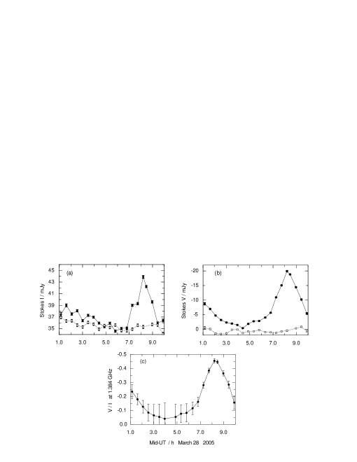
Figure 2: The Stokes I and V flux densities from the 25 min integrations on March 28 2005 are plotted against the mid-UT of each integration. Panel (a) shows the I flux densities at 1.384 GHz (filled circles joined by full lines) and the I flux densities at 2.368 GHz (open squares joined by dotted lines). Panel (b) shows the V flux densities at 1.384 GHz (filled circles joined by full lines) and at 2.368 GHz (open squares joined by dotted lines). Panel (c) chows the corresponding fractional values of circular polarisation (V/I) with their error bars. The error bars attached to the 1.384 GHz flux densities in panels (a) and (b) are the rms residuals from the task UVFIT; the error bars at 2.368 GHz are not shown but are similar in amplitude.

2.3 Modulation index for March 28 2005

The modulation indices for the coherent emission of 28 March are plotted in Figure 3a, which shows a steadily increasing value for M as the integration time falls to 0.078 s. It seems probable that M will approach 100% at still lower values of integration time, suggesting that temporal structure as low as the 2–3 ms seen at times by Osten and Bastian (2007) may be present. However, the presence of such fine temporal structure does not necessarily discriminate between the alternative mechanisms of plasma emission and ECME. Additional attributes of the radiation such as its fractional instantaneous bandwidth and its frequency drift rate are necessary in making this distinction.

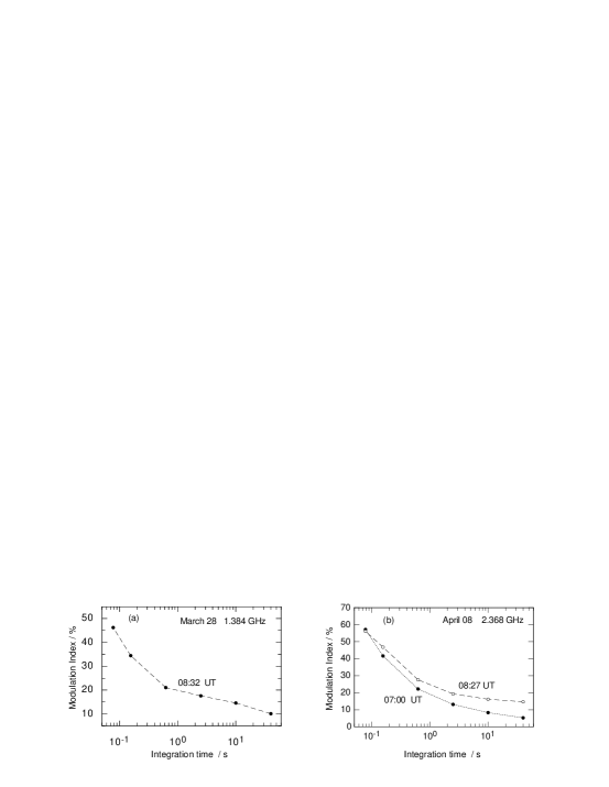
Figure 3: Plots of modulation index (defined by equation (3) in Section 2.2) versus integration time for the high-time resolution sampling at 78 ms. Panel (a) shows the relationship for the 1.384 GHz sample centred on 08:32 UT on March 28 2005. Panel (b) shows the relationships derived from two intervals of 2.368 GHz coherent emission centred on 07:00 and 08:27 UT on April 08 2005.

2.4 Observations of April 08 2005

Figure 4 shows the total and polarised flux densities for the 8-h observation of April 08 in panels (a) and (b) respectively, while panel (c) plots the polarised fraction V/I. It is evident that a significant event occurred at 2.368 GHz in the last three hours of the observation, but on this date there was also a slowly decreasing level of left-handed circular polarisation at 1.384 GHz (negative Stokes V). In this respect, the emissions differ significantly from those on March 28, when the stonger event occurred at 1.384 GHz and a negligible level of Stokes V was seen at 2.368 GHz.

The intensity levels of Stokes V at 1.384 GHz were never high enough to actuate the high-time resolution sampling, but we were able to record two high-resolution sections at 2.368 GHz centred on 07:00 UT and 08:27 UT. The Stokes I and V flux densities were similar to those attained on March 28. The two high-resolution sections were binned in the same manner as that described in Section 2.2 and their modulation indices (M) were computed.

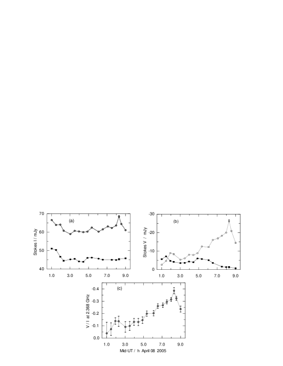
Figure 4: The Stokes I and V flux densities from the 25 min integrations on April 08 2005 are plotted against the mid-UT of each integration. The description of the three panels is identical to that of the caption to Figure 2.

2.5 Modulation indices for April 08 2005

Figure 3b shows that the modulation indices steadily increase with decreasing integration time and are still increasing at our resolution limit of 78 ms. A comparison of Figures 3a and 3b indicates that the modulation indices of the 1.384 and 2.368 GHz coherent emissions show similar behaviour. Unfortunately, we do not have the capability to increase our time and frequency resolution for continuum observations with the existing ATNF correlator; such observations would be required to better differentiate between possible coherent emission mechanisms.

3 The spectral structure in coherent emission

The IF output of the ATCA consisted of 13 independent frequency channels, each of 8 MHz width and spaced 8 MHz apart, permitting us to display the radio spectrum over a total width of 104 MHz. For this task we refer to the 25 min integrations of the Stokes V data in Figures 2b and 4b, confining our attention to the several integrations that comprise the most highly polarised sections in these two figures. In this spectral analysis we can utilize both low and high time resolution integrations. The task UVSPEC in the MIRIAD software was used to compute the averaged Stokes V and I flux densities and their errors in each of the 8 MHz-wide channels for the selected integrations. These flux densities were then plotted against the mid-frequency of each channel.

3.1 The spectra on March 28

Figure 5 shows the spectral structure and its dynamic behaviour at 1.384 GHz over the seven 25 min integrations that form the highly polarised event in Figure 2b. The high time resolution data is centred on the panel labelled 08:28 UT; here we show both the Stokes I and V spectra. The Stokes I spectrum closely mimics the Stokes V in the remainder of the panels. The increase in Stokes V is within a few percent of that in Stokes I in the seven panels, with an average value of ($\Delta{V}/\Delta{I}$) = 0.99 (weighted by variance^-1). Thus, as far as we can determine, the emission is 100% circularly polarised in the left-handed sense.

The details from successive frames clearly suggest that bursts of highly polarised emission drift relatively slowly through the total 104 MHz bandwidth at $\sim$0.7 MHz min^-1. If one fixes attention on the burst in the top left panel, we note that by 07:16 UT it has drifted along the frame to lower frequencies. By 07:44 UT, this burst has practically drifted below 1.34 GHz and another burst of $\sim$45 MHz to FWHM has appeared near the high frequency end of the band. At 08:28 UT this new burst is situated near the centre of the band and by 08:58 is approaching the low frequency end. By 09:26 UT it has reached the low frequency end of the band.

The instantaneous bandwidth of the coherent emission is one of the critical parameters in any theoretical mechanism for its creation. The FWHM of the most completely delineated burst at 08:28 UT is 48 MHz, yielding a value of ($\Delta\nu/\nu$)=0.035. This, however, is an upper limit because in the 22 min integration, from which the panel is constructed, the centre frequency of the emission should have drifted $\sim$15 MHz. Therefore, the true instantaneous FWHM is likely to be $\sim$30 MHz, giving ($\Delta\nu/\nu)\sim$ 0.02. We note that Stokes V never falls completely to zero in any of the panels, because there are always remnants of the preceding and following bursts occupying one or other of the ends of the 104 MHz bandwidth of the receiver. If the channel bandwidth could be reduced to say 4 MHz, one might see that zero Stokes V is reached between bursts, although that would depend on how regularly they are generated.

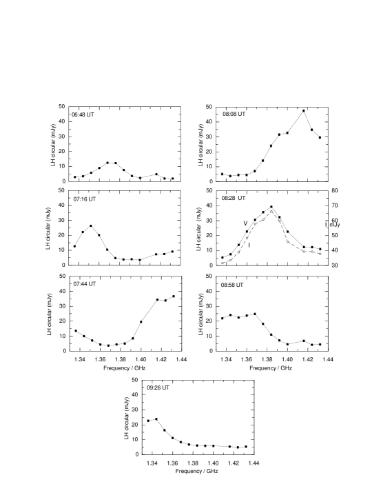
Figure 5: The spectral structure in the highly polarised 1.384 GHz data of March 28 across the 104 MHz bandwidth of the compact array. The panels are arranged in increasing values of mid-UT of the 25 min integrations making up the data. Six of the 7 panels show the structure in Stokes V only, but the panel at 08:28 UT is derived from the high-time resolution sampling and shows both the Stokes I and V spectral structure. The frequency channel at $\sim$1.41 GHz is missing due to an interference problem. The errors in the flux measurements are similar to that shown in Figure 6.

3.2 The spectra on April 08

Figure 6 shows the spectral structure at 2.368 GHz over the nine 25 min integrations that contribute to the highly polarised event in Figure 4b. Data with high time resolution were recorded in the panels labelled 07:05 UT and 08:33 UT; in the latter we show both the Stokes I and Stokes V data on the same intensity scale spacings. The Stokes I and V spectra are very similar in shape and amplitude on all these scans. The larger error bars in the panel labelled 08:18 UT are due to this integration having been cut short in order to begin the high time resolution observations that contribute to the next panel. The increase in Stokes V and I are very similar with an average value of ($\Delta{V}/\Delta{I}$) = 0.99 (weighted by variance^-1). Again, as for the observations of March 28, the emission is polarised at close to 100% in the left-handed sense.

The successive panels of Figure 6 show that although spectral structure is clearly present in the 2.368 GHz polarised emission, it is difficult to assign a direction of drift. Unlike the drifting narrow-band bursts visible at 1.384 GHz in Figure 5, no individual burst can be completely isolated. This is no doubt due to the much wider bandwidth occupied by the 2.386 GHz polarized bursts. The FWHM bandwidth of these bursts is probably closer to twice our 104 MHz bandwidth, and one would need to be able to trace the intensity structure over at least this frequency interval to decide on its direction of drift. One notes that the polarised emission does not fall to near zero in any of these panels, indicating the presence of pronounced frequency overlapping of adjacent bursts.

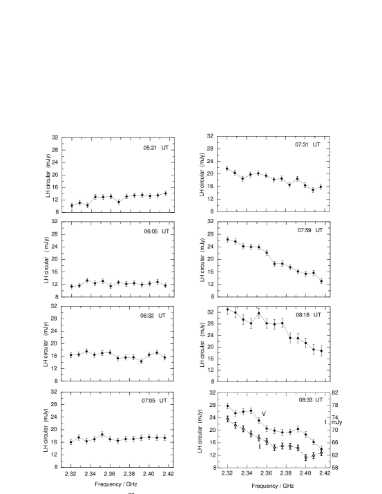
Figure 6: The spectral structure in the highly polarised 2.368 GHz data of April 08 across the 104 MHz bandwidth of the compact array. The panels are arranged in increasing values of mid-UT of the 25 min integrations making up the data. Eight of the nine panels show the structure in Stokes V only, but the panel at 08:33 UT is derived from high-time resolution sampling and shows the spectral variation in both Stokes I and V.

3.3 Orbital phase dependence

VLBA observations of HR 1099 by Ransom et al. (2002) provide reasonable evidence that during times of high radio activity the magnetospheres of the binary components had a high degree of interaction such that two compact 8.4 GHz sources were seen, the stronger source centred on the K2 sub-giant and the weaker on the G5 dwarf. If our highly polarised coherent emission were to also originate near the G5 dwarf at times of enhanced activity, one may expect that the phase dependencies of the two phenomena would be similar.

We have searched the literature to determine the epochs of other events of long-lasting coherent emission from HR 1099 (greater than one hour in duration and Stokes V $\sim$100%). Table 1 gives the result of phase binning the eight occurrences of such emission. Although the statistics are rather poor, this table shows that there has been a definite tendency for the coherent events to favour the orbital phase range 0.33–0.83 with a minor peak in the phase range 0.50–0.67. Ransom et al. (2002) used the same orbital ephemeris to derive the phase range over which they observed the 8.4 GHz source near the G5 dwarf to move from 0.72–0.76. The secondary source was already at full strength at the start of their observations, so the phase range could be credibly extrapolated to earlier phases to coincide with the peak in the coherent emission in Table 1. This coincidence in phase range will be discussed in Section 5.

Phase	No. of Events	Ref
0.0–0.17	0
0.17–0.33	1	(1)
0.34–0.50	2	(1,2)
0.50–0.67	3	(1,2,3)
0.67–0.83	2	(2,3)
0.83–1.00	0

Table 1: The phase dependance of the ECME events. We have used the ephemeris of Fekel (1983) to determine the orbital phase of the events. References: (1) Osten et al (2002), (2) Jones et al (1993), (3) this paper.

4 Summary of observational results

The following observational conclusions can be drawn from our data:

1. Highly circularly polarised emission ($\sim 100\%$ left-hand) was seen in two observing sessions separated by 11 days.

2. The intervals of strong, highly polarised emission lasted from 2–3 hrs (Figures 2 & 4).

3. In the first observing epoch, the highly polarised emission was seen only at 1.384 GHz (Figure 2).

4. During the second epoch observation, a strong, highly polarized event was observed at 2.368 GHz, with weaker, highly polarised 1.384 GHz emission partially overlapping the stronger 2.368 GHz emission (Figure 4).

5. Three 22 min integrations were made at high time resolution (0.078 s), enabling us to show (Figure 3) that the modulation index of the Stokes V intensity increased as the integration time was reduced and was still increasing at our resolution limit.

6. During the first epoch event, coherent emission at 1.384 GHz contained a regular frequency structure of bursts with FWHM width of $\sim$48 MHz that drifted across the spectrum at $\sim$0.7 MHz min^-1 (Figure 5) . The second epoch of coherent emission at 2.368 GHz also contained definite spectral structure (Figure 6), but its significantly wider FWHM did not permit an accurate estimate of its bandwidth nor its direction of frequency drift.

7. The two long-lasting coherent events reported in this paper conform with six others reported in the literature, occurring preferentially in the orbital phase range of 0.50–0.67.

5 Discussion

It is well known that coherent radio emission is emitted from a variety of celestial objects ranging from the Sun, Earth, Jupiter and Saturn to flare stars and some close binaries. In the case of the Sun (Melrose & Dulk 1982), in the flare star AD Leo (Lang et al. 1983), and in the flare star YZ CMi (Lang & Wilson 1988), high time resolution measurements have shown temporal structure of tens of millisec, which indicates from a light-travel time argument that the linear size of the emitting region should be only a few times $3\times 10^{8}$ cm.

First, we check the peak brightness temperatures reached by these highly polarised bursts, using a convenient formula due to Osten and Bastian (2007):

$$T_{B}=6\times 10^{14}S_{mJy}(D_{pc}/\nu_{GHz}\Delta{t_{ms}})^{2}$$ (4)

Where $S_{mJy}$ is the peak polarised flux density, $D_{pc}$ is the stellar distance, (29 pc) $\nu_{GHz}$ is the frequency and $\Delta t_{ms}$ is the burst duration, here taken as the time resolution of the sampling (78 ms).

In the first epoch observation at 1.384 GHz, the maximum polarised flux of 48 mJy (see Figure 5) results in $T_{B}>2.1\times 10^{15}$ K. In the second epoch observation at 2.368 GHz, the maximum polarised flux density of $>$ 32 mJy (see Figure 6) yields $T_{B}>4.7\times 10^{14}$ K. If the temporal structure in these bursts is as low as 5–10 ms, the brightness temperatures would be two orders of magnitude higher. It is clear that this completely polarised emission can not be due to an incoherent mechanism such as that producing thermal emission or gyro-synchrotron radiation.

Next, it is important to compare the total time intervals of coherent emission on a M4 V flare star (AD Leo) and the close binary HR 1099 of spectral type K3 IV + G5 V. Our Figures 2 and 3 show that the events on HR 1099 last for 2–4 hrs as compared to   1 min for the flares reported by Osten and Bastian (2006, 2007). One questions whether this more than two orders of magnitude difference can be compatible with the same mechanisms operating in sources with similar linear sizes, coronal electron densities and magnetic fields in two very dissimilar stellar systems.

Perhaps the analysis of Osten and Bastian (2006) in their Figure 6 of a moderate intensity, 60 s flare on AD Leo in the frequency range 1162–1568 MHz is the most suitable to compare with the results for HR 1099 in our Figure 5. Osten and Bastian have plotted their results with a degraded time resolution of 200 ms and a degraded frequency resolution of 7.8 MHz. Our data are plotted with a time resolution of 78 ms and frequency resolution of 8.0 MHz. The important conclusions to come from this comparison are the frequency drift rates of the bursts and their instantaneous bandwidths. Osten and Bastian find a drift rate of 52 MHz s^-1, while for HR 1099 we measure a frequency drift rate of $\sim$0.012 MHz s^-1, i.e. more than 3 orders of magnitude slower, although the direction of drift is from high to low frequencies in both experiments. A second significant difference between the two sets of data is the instantaneous bandwidth of the bursts; in AD Leo, $\Delta\nu/\nu$$\buildrel{\lower 3.0pt\hbox{$>$}}\over{\lower 2.0pt\hbox{$\sim$}}$0.29, while in HR 1099, $\Delta\nu/\nu\sim$0.036 a difference of a factor of $\sim$8. The third outstanding difference between the above sets of data is the difference in burst occurrence rates. In their Arecibo data of June 2003, Osten and Bastian (2006) detected only two short (60 s) bursts in 16 hr of data, spread over four days. In our HR 1099 data of March 28 2005, we see two long-lasting intervals of coherent emission, with the more intense episode consisting of two distinct bursts slowly traversing our 104 MHz band width. Our bursts may contain much finer structure that is smoothed out by our 78 ms time resolution, but its absence in our data makes a comparison with the higher resolution data of Osten and Bastian (2007) a less-fruitful exercise.

Perhaps an even more relevant comparison may be made between our data and the slowly varying decimetric coherent emission from the dMe flare star YZ CMi (Lang & Wilson 1988). The emission lasted for $\sim$5h and consisted of a number of discrete bursts, each of $\sim$10 min duration and 100% polarised in the left-handed sense. Four of these bursts were shown to contain narrow-band structure with a fractional bandwidth of $\Delta\nu/\nu=$0.02, but their integration time of 10 s did not permit the authors to investigate their temporal structure. The authors place an upper limit of $<$ 0.05 MHz s^-1 on the frequency drift of these bursts, a value consistent with our first epoch value of 0.012 MHz s^-1. The alternative mechanisms of ECME and plasma emission are discussed, but no definite preference was given.

Comparing the properties of the coherent emission which we have detected in HR 1099 with that from other stellar systems, we favour ECME as a more likely mechanism for our HR 1099 emission because: (1) its 100% polarisation is much higher than that achieved in most solar burst of Types I–V; (2) its duration is much longer than all solar bursts except Type IV; (3) its frequency-drift rate is orders of magnitude lower than solar bursts and the short flares from AD Leo reported by Osten and Bastian (2006, 2007); (4) its temporal structure is much finer than that found in solar bursts, except perhaps that in Type 1 solar noise storms and in the solar decimetric ‘spike’ emission.

Regarding the location of the coherent source in the close binary, we must consider at least two possibilities: (1) in the corona of either of the components; (2) a coherent source resulting from the interaction between the magnetospheres of the components. We shall consider both options below.

5.1 The single-star source of coherent emission

It is tempting to interpret our highly polarised and highly time-structured microwave emission in terms of solar analogues, which have been studied most extensively at metric and decimetric wavelengths and are described comprehensively in the book ‘Solar Radiophysics’ edited by McLean and Labrum (1985). Whether one can apply the models developed for solar bursts of Types I–V and their associated continuum emissions to a binary consisting of stars of differing spectral types is open to serious question. The solar Type I noise storm has the long duration, high polarisation and fine intensity structure that most resembles our emissions from HR 1099, but this is confined to metre waves – we do not, therefore consider this a likely cause for the events we have detected in HR 1099.

The so-called solar ‘spike bursts’, emitted in the frequency range 0.3–3 GHz, possess similar fine time and frequency structure to that contained in the coherent emission from HR1099 and are highly polarised, suggesting that such a source in the corona of either of the binary components is a distinct possibility. The most frequently discussed driver of solar spike bursts is an anisotropy in the pitch angle distribution about magnetic field lines, commonly called ‘the loss-cone’, producing an electron-cyclotron maser.

First, it must be noted that one necessary condition for an electron cyclotron maser to operate is that the source-region plasma has a relatively low plasma density and/or a relatively high magnetic field strength, such that the ratio of the electron plasma frequency, $\nu_{p}=8.98\times 10^{3}n_{e}^{1/2}$ MHz to the electron-cyclotron frequency, $n_{c}$ = 2.80 H MHz, is small; here, H is the magnetic field strength in gauss and $n_{e}$ the electron density cm^-3. For $\nu_{p}/\nu_{c}<<$ 1, the highest maser growth rate is in the x-mode at the fundamental ($\nu\sim\nu_{p}$), but it is highly likely that fundamental maser emission would be reabsorbed as it propagates into harmonic absorption bands in regions with lower magnetic field strengths. Consequently, the strongest maser emission likely to reach the observer is x-mode emission at the second harmonic (Melrose & Dulk 1982). However, without knowledge of the predominant magnetic field polarity of the active region producing the radiation, the polarisation mode (x-mode or o-mode) cannot be ascertained from the observed handedness. Second-harmonic emission at 1.4 GHz corresponds to a source region field of 250 G, and the condition $\nu_{p}/\nu_{c}<$ 1 then requires source region plasma densities $<6\times 10^{9}$ cm^-3. This plasma density requirement can be met almost anywhere in the stellar corona – even at the low coronal height of 1.003 $R_{\odot}$ the Baumbach-Allen model of the solar corona (Allen 1973) yields a plasma frequency of only 183 MHz, well below either of our observing frequencies of 1.384 and 2.368 GHz. Plasma densities will, of course, be enhanced in the converging magnetic field lines of coronal loops near their footprints.

At this point, we may consider whether the source models developed to account for the observed auroral kilometric radiation (AKR) could be of assistance in interpreting the coherent sources in HR 1099. The instructive reviews by Ergun et al. (2000), and Treumann (2006) show that AKR electron-cyclotron emission was measured by satellites that actually traversed the auroral source cavities, allowing detailed theoretical models to be checked by measurements of AKR frequency, polarisation mode, plasma frequencies, magnetic and electric field strengths and the temporal and frequency structure of AKR.

These authors find that, although a loss cone is generated, it is insufficient to amplify the AKR waves to levels that could account for the high-brightness, fine structured sources within the cavity. They propose an alternative driver, consisting of an unstable ‘horse-shoe’ or ‘shell’ distribution of fast electron velocities with respect to converging field lines in the presence of a parallel electric field and a generally low plasma density, referring to this source region as the ‘auroral cavity’. In this case, the direction of the earth’s field is known with respect to the satellite’s path through the region and so the polarisation mode can be identified. The horse-shoe distribution is apparently a much more efficient way of increasing the growth rate of AKR, which is preferentially emitted perpendicular to the magnetic field lines in the right-hand circularly polarized x-mode. Just as importantly, the fundamental of the electron-cyclotron frequency can escape the cavity, yielding a much stronger observed intensity of AKR than would have been observed with the loss-cone model.

Other characteristics of the AKR that mimic the coherent emission from HR 1099 include its fine temporal and frequency structure. Bursts of AKR with fractional bandwidth as low as 0.01 and temporal structure of 100 ms can drift through the spectrum at various rates, but a good example is shown in Treumann’s Figure 6 . This illustrates a consistent drift from high to lower frequencies of 7–8 kHz s^-1, comparing well with the drift rate of the coherent event in our Figure 5 of $\sim$12 kHz s^-1 from high to lower frequencies. However, we should be cautious in applying the auroral model to stellar coronae, where we are dealing with magnetic fields and ambient plasma densities that are orders of magnitude higher than auroral values. Nevertheless, the aforementioned similarities suggest that this model should be explored in detail for stellar coherent emission. It is feasible that source regions having aurora-like general structure could be found in the converging magnetic field lines of coronal loops, but detailed modelling using realistic field strengths and plasma densities is required to validate this proposal.

5.2 The two-star coherent source

If the observed coherent radiation from HR 1099 is due to the interaction between the magnetospheres of its components it would seem that the more active K2 subgiant could possess a strong stellar wind capable of transferring a relatively dense plasma with imbedded magnetic field to the corona of the G5 dwarf. Ransom et al’s (2002) VLBA maps show that a relatively weaker 8.4 GHz gyro-synchrotron source was detected near the position of the G5 star only when the system was in a state of high activity. A mapping of four equal subdivisions of the data resulted in this source moving its position in a manner consistent with the orbital motion of the G5 dwarf about the K2 subgiant. We have noted in section 3.3 that the orbital phases at which the published coherent events were detected appear to favour an orbital phase range falling within that deduced from the positions of the secondary 8.4 GHz source.

The fact that no 8.4 GHz coherent emission was detected from either star during this observation by Ransom et al. does not rule out its presence at considerably lower frequencies. All occurrences of coherent radiation from HR 1099 have been detected at frequencies below 5 GHz, usually at about 1.4–2.4 GHz, where most lower frequency observations have been made. Gyro-synchrotron emission of comparable strength often coexists with the coherent emission as our Figures 2 and 4 demonstrate, but, although this does not mean that the two radiation types necessarily emanate from the same source region in the corona, they could have a common exciting agent.

Considering the geometry and phase dependence of the coherent events as compared with that of Ransom et al’s secondary source, we propose that an auroral analogue may operate, in which comparatively dense plasma is transferred from the stellar wind of the K2 subgiant into the poloidal field of its companion. The dwarf’s magnetic poles would likely be visible, due to the low inclination (38 degrees) of the orbital plane to the sky. Field strengths near these poles would be considerably higher than for the Sun, due to the much more rapid rotation rate. However, we stress again that a thorough modelling of the situation needs to be done before the auroral analogue can be established.

5.3 Slow changes in the intensity and spectral distribution

Figures 2 and 4 demonstrate that both intensity and spectral parameters vary over an interval of nine hours and from day to day. In March 2005 (Figure 2) the coherent event was confined to $\sim$1.4 GHz and varied in intensity by a factor of ten between the two peaks separated by at least 7 h. Our poor angular resolution does not permit us to decide whether the two peaks are due to separate coronal sources or whether the plasma density and/or magnetic field strength varies within the one maser source. A VLBI network with an angular resolution of $\sim$one milliarcsec at 1.4 GHz will eventually be able to decide between these alternative interpretations.

Figure 4 (for April 2005) illustrates a phenomenon that has not been reported hitherto. Here we observe that coherent radiation is present simultaneously at widely separated frequencies. At $\sim$1.4 GHz its intensity drops continuously to almost zero over the 8 h observation, while at $\sim$2.4 GHz its intensity rises continuously to a peak near the end of the observation; there is little, if any, correlation between the intensities at the two frequencies, suggesting that two separate coherent sources are operating independently and with differing plasma densities and/or magnetic field strengths. In order to resolve this dilemma, one is faced with the task of simultaneously operating a VLBA network at two widely separated frequencies to achieve an angular resolution of $\sim$one milliarcsec at the lower frequency. Such angular resolutions could be achieved at these decimetric wavelengths by a satellite operating with a network of earthbound radio telescopes.

6 References

Allen, C..W. 1973, Astrophysical Quantities, 3rd edition, p176, The Athlone Press
Dulk, G.A., 1985, Ann. Rev. Astron. Astrophys., 23, 169
Ergun, R.E., et al. 2000, ApJ, 538, 456
Hallinan, G., et al. 2007, ApJ, 663, L25
Jones, K.L., Brown, A., Stewart, R.T., Slee, O.B. 1996, MNRAS, 283, 1331
Fekel, F.C., 1983, ApJ, 268, 274
Lang, K.R, Wilson, R.F. 1988, ApJ, 326, 300
Lang, K.R. et al. 1983, ApJ (Letters), 272, L15
Osten, R.A. et al. 2004, ApJS, 153, 317
Osten, R.A., Bastian, T.S. 2006, ApJ, 1016
Osten, R.A., Bastian, T.S.. 2007, astro-phys, arXiv:0710.5881
Melrose, D.B., Dulk, G.A. 1982, Ap.J, 259, 844
McLean, D.J., Labrum, N.R. eds, 1985, Solar Radiophysics, CUP
Ramsay, G. et al. 2007, MNRAS, 382, 461
Ransom, R.R. et al. 2002, ApJ, 572, 487
Slee, O.B., Willes, A.J., Robinson, R.D. 2003, PASA, 20, 257
Treumann, R.A. 2006, Astron Astrophys. Rev., 13, 229
White, S.M., Franciosini, E. 1995, ApJ, 444, 342
Willes, A.J., Wu, K. 2004, MNRAS, 348, 285
Wu, K., Cropper, M., Ramsay, G., Sekiguchi, K. 2002, MNRAS, 331, 221