Temporal evolution of thermal emission from relativistically expanding plasma

Abstract

Propagation of photons in relativistically expanding plasma outflows, ejected from a progenitor characterized by steady Lorentz factor $\Gamma$ is considered. Photons that are injected in regions of high optical depth are advected with the flow until they escape at the photosphere. Below the photosphere, the photons are coupled to the plasma via Compton scattering with the electrons. I show here, that as a result of the slight misalignment of the scattering electrons velocity vectors, the (local) comoving photon energy decreases with radius as $\varepsilon^{\prime}(r)\propto r^{-2/3}$. This mechanism dominates the photon cooling in scenarios of faster adiabatic cooling of the electrons. I then show that the photospheric radius of a relativistically expanding plasma wind strongly depends on the angle to the line of sight, $\theta$. For $\theta\lesssim\Gamma^{-1}$, the photospheric radius $r_{ph}$ is $\theta$-independent, while for $\theta\gtrsim\Gamma^{-1}$, $r_{ph}(\theta)\propto\theta^{2}$. I show that the $\theta$-dependence of the photosphere implies that for flow parameters characterizing gamma-ray bursts (GRBs), thermal photons originating from below the photosphere can be observed up to tens of seconds following the inner engine activity decay. I calculate the probability density function $P(r,\theta)$ of a thermal photon to escape the plasma at radius $r$ and angle $\theta$. Using this function, I show that following the termination of the internal photon injection mechanism, the thermal flux decreases as $F_{BB}^{ob.}(t)\propto t^{-2}$, and that the decay of the photon energy with radius results in a power law decay of the observed temperature, $T^{ob.}(t)\propto t^{-\beta}$, with $\beta=2/3$ at early times, which changes to $\beta\simeq 1/2$ later. Detailed numerical results are in very good agreement with the analytical predictions. I discuss the consequences of this temporal behavior in view of the recent evidence for a thermal emission component observed during the prompt emission phase of gamma-ray bursts.

1. Introduction

Evidence for relativistic expansion in plasma winds exist in various astronomical objects, such as microquasars (Mirabel & Rodriguez, 1994; Hjellming & Rupen, 1995), active galactic nuclei (AGNs; Lind & Blandford, 1985; Gopal-Krishna et al. , 2006) and gamma-ray bursts (GRBs; Paczyński, 1986; Goodman, 1986). In many of these objects, the density at the base of the flow is sufficiently high, so that the optical depth to Thomson scattering by the baryon-related electrons exceeds unity. If the optical depth to scattering is high enough, the emerging spectrum of photons emitted by radiative processes occurring at or near the base of the flow is inevitably thermal or quasi-thermal (a Wien spectrum could also emerge if the number of photons is conserved by the radiative processes). These photons escape the flow once they decouple from the plasma, at the photosphere (e.g., Paczyński, 1990).

The photosphere is usually defined as a surface in space which fulfills the following requirement: the optical depth to scattering a photon originating from a point on this surface and reaching the observer is equal to unity. Therefore, calculation of the position of this surface requires knowledge of the density profile between this surface and the observer (and, in principle, knowledge of the photon energy and the velocity profile, since the cross section is energy dependent; however, I will neglect these effects). Calculation of the photospheric surface in the case of steady, spherically symmetric, relativistic wind was carried out by Abramowicz et al.  (1991). In this work, it was found that the position of the photosphere has a complicated, non-trivial shape which strongly depends on the viewing angle and the wind Lorentz factor $\Gamma$. This shape can be described analytically (see Abramowicz et al. , 1991, eq. 3.4). For spherically symmetric wind, the photospheric surface is symmetric with respect to rotation around the axis to the line of sight. Thus, I will use the term “photospheric radius” from here on to describe its position in space, noting that the photospheric radius is a function of the angle to the line of sight, $r_{ph}=r_{ph}(\theta)$.

While the optical depth to scattering from the photospheric radius $r_{ph}(\theta)$ to the observer is by definition $\tau(r_{ph}[\theta])=1$, in fact photons have a finite probability of being scattered at any point in space in which electrons exist. Since in every scattering event a photon changes its propagation direction and its energy, the observed flux and temperature of the thermal photons depend on the last scattering position, scattering time, the comoving temperature at this position, and last scattering angle. A full description of the last scattering position and scattering angle can only be done in terms of probability density function $P(r,\theta)$. The probability density function is an extension of the standard use of the photospheric radius as a surface in space from which thermal photons emerge, to consider the finite probability of a photon to emerge from an arbitrary radius $r$ and arbitrary angle $\theta$.

Once the probability of a thermal photon to emerge at time $t$ from radius $r$ and angle $\theta$ is known, the observed flux of the thermal photons can be calculated. The first observed (thermal) photon originates from the radial axis towards the observer (on the line of sight). At later times an observer sees photons that originate from increasingly higher angles to the line of sight and from larger radii. The observed thermal flux thus varies with time.

The observed temperature of thermal photons emerging from radius $r$ at angle to the line of sight $\theta$ is blue shifted due to the Doppler effect, $T^{ob.}={\mathcal{D}}T^{\prime}(r)$. Here, $T^{\prime}(r)$ is the photon temperature in the comoving frame, $T^{ob.}$ is the observed temperature, ${\mathcal{D}}\equiv[\Gamma(1-\beta\mu)]^{-1}$ is the Doppler factor, $\beta c$ is the fluid velocity and $\mu=\cos(\theta)$. Photons emitted on the line of sight are blue shifted by ${\mathcal{D}}_{0}={\mathcal{D}}(\theta=0)\simeq 2\Gamma$ (the last equality holds for $\Gamma\gg 1$), while photons that originate from $\theta>0$ are blue shifted by Doppler factor ${\mathcal{D}}(\theta>0)<{\mathcal{D}}_{0}$. Note that ${\mathcal{D}}(\theta)$ is a monotonically decreasing function of $\theta$.

The photon comoving temperature $T^{\prime}(r)$ varies with the radius below the photosphere. At $r<r_{ph}$, photons are coupled to the flow by multiple Compton scattering. Therefore, once thermalize, the photons comoving temperature is equal to the electrons comoving temperature $T_{el}^{\prime}(r)$ ($T_{el}^{\prime}$ is measured in units of $m_{e}c^{2}$). The electrons comoving temperature changes as they propagate downstream, due to adiabatic energy losses and possible internal heating mechanisms that are coupled to the flow. The photon temperature is thus expected to trace the electrons temperature. However, as I will show below, an additional mechanism determines the photon temperature below the photosphere. This mechanism is based on photon energy losses due to the misalignment of the scattering electrons velocity vectors in regions of high optical depth, and leads to photon comoving temperature decay as a power law in radius, $T^{\prime}(r)\propto r^{-2/3}$ (in the limit of relativistic outflows, characterized by Lorentz factor $\Gamma\gg 1$). Therefore, as long as the electrons comoving temperature does not drop faster than $T_{el}^{\prime}(r)\propto r^{-2/3}$, the photon comoving temperature traces the electrons comoving temperature. However, if adiabatic energy losses cause the electrons comoving temperature to decay faster than $r^{-2/3}$, than the mechanism described below limits the photon comoving temperature to decay as $r^{-2/3}$. In this case, the photon comoving temperature does not follow the electrons temperature.

The mechanism by which photons lose their energy below the photosphere is solely based on 2- and 3-dimensional scattering geometry. In every scattering event, the direction of the photon propagation vector slightly changes, as the average scattering angle $\langle\theta\rangle\sim\Gamma^{-1}$. Therefore, in every consequent scattering, a photon is being scattered by electrons whos direction vectors are slightly misaligned. This misalignment, in turn, inherently leads to photon energy losses, regardless of the comoving temperature of the electrons. This effect can best be understood if one considers the rest frame of the first scatterer. Assuming that in this frame the comoving photon energy is very low, $\varepsilon^{\prime}\ll m_{e}c^{2}$, the (comoving) outgoing photon energy is nearly equal to its energy before the scattering, independent on the scattering angle. The misalignment of the electrons velocity vectors implies that for scattering angles which are different than $(0,\pi)$, the velocity vector of the next scatterer points outward. Thus, the comoving energy of the photon in the rest frame of the second scatterer is slightly lower than its comoving energy in the rest frame of the first scatterer. As I will show below, for constant outflow velocity characterized by Lorentz factor $\Gamma\gg 1$, this effect results in a power law decay of the comoving photon energy, $\epsilon^{\prime}(r)\propto r^{-2/3}$. This decay, in turn, results in a decrease of the observed temperature at late times.

Transient physical sources have a finite emission duration, during which their inner engine is active. Therefore, at any given observed time $t^{ob.}>0$, an observer sees simultaneously photons originating from a range of radii and a range of angles to the line of sight, $\theta_{\min}\leq\theta\leq\theta_{\max}$. The dependence of the photon comoving temperature on the photospheric (last scattering event) radius and the dependence of both the photospheric radius and the Doppler factor on the angle $\theta$ to the line of sight thus lead to the conclusion that thermal emission (Planck spectrum) in the comoving frame is observed as a modified black body. However, the observed spectrum is a convolution of black body spectra observed with different fluxes and temperatures, and as such does not differ much from a black body.

As long as the inner engine is active, the observed flux and temperature are dominated by photons emitted on axis (on the line of sight). Following the decay of the inner engine, the flux becomes dominated by photons emitted from increasingly higher angles and radii (the curvature effect, also known as “the high latitude emission” effect; see, e.g., Fenimore, Madras & Nayakshin, 1996; Kumar & Panaitescu, 2000; Ryde & Petrosian, 2002; Dermer, 2004, for discussions on this effect in optically thin emission models). Considering the optically thin cases, the results obtained in these works are not valid for the scenario considered here, of thermal emission from optically thick expanding plasma.

The main goal of this paper is to provide a theoretical framework for the analysis of thermal emission from astrophysical transient characterized by relativistic outflows, and to calculate the expected observed thermal flux and temperature at late times, following the decay of the inner engine. A key motivation to this work are the results obtained by Ryde (2004, 2005), of a decaying thermal component observed during the prompt emission phase of GRBs. In these works, it was shown that after $\sim 1-3$ s the temperature of the thermal component decreases as a power law in time, $T^{ob.}\propto t^{-\alpha}$, with power law index $\alpha\simeq 0.6-1.1$. An additional analysis (F. Ryde & A.Pe’er 2008, in preparation) shows that after a short rise, the flux of the black body component of these bursts also decreases with time as $F_{BB}^{ob.}\propto t^{-\beta}$, with power law index $\beta\approx 2.0-2.5$. I show here that these results are naturally obtained in a model which considers the full spatial scattering positions and photon scattering angles (given by the probability distribution function $P[r,\theta]$) and takes into consideration the comoving energy losses of the photons below the photosphere, due to the slight misalignment of the scattering electrons.

This paper is organized as follows. I first calculate in §2 the optical depth at every point in space for scattering into angle $\theta$, under the assumption of relativistic, steady outflow. From this calculation, I find the angular dependence of the photospheric radius, $r_{ph}(\theta)$. The calculation in this section closely follows the treatment by Abramowicz et al.  (1991), although it is somewhat more general since in this work the results were not presented as a function of the viewing angle, $\theta$. For parameters characterizing GRBs, it is shown in §2.1 that thermal emission can be observed up to tens of seconds. The results obtained in this section are used in §3 in which the theory of photon energy loss due to misalignment of the scattering direction vectors below the photosphere is developed. The probability density function $P(r,\theta)$ of a photon to be scattered from radius $r$ and angle $\theta$ is introduced in §4. In this section, I calculate the expected flux and temperature of the thermal emission, and show that following the termination of the inner engine, the thermal flux and temperature decay as power law in time, $F\propto t^{-\alpha}$, and $T^{ob.}\propto t^{-\beta}$, with $\alpha=2$ and $\beta=2/3$ at early times, modified into $\beta\simeq 0.5$ later. The numerical model is presented in §5. The Monte-Carlo simulation provides full calculation of photon propagation in relativistically expanding plasma, and is used to validate the approximations of the analytical calculations. The numerical results are compared to the analytical predictions, and are found to be in very good agreement. I summarize the results and discuss their consequences in §6.

2. Optical depth and photospheric radius in relativistically expanding plasma wind

Following the treatment of Abramowicz et al.  (1991), I consider the ejection of a spherically symmetric plasma wind from a progenitor characterized by constant mass loss rate $\dot{M}$, that expands with time independent velocity $v=\beta c$. The ejection begins at $t=0$ from radius $r=0$, thus at time $t$ the plasma outer edge is at radius $r_{out}(t)=\beta ct$ from the center. For constant ${\dot{M}}$ and $\Gamma$, at $r<r_{out}$ the comoving plasma density is given by $n^{\prime}(r)={\dot{M}}/(4\pi m_{p}v\Gamma r^{2})$, where $\Gamma=(1-\beta^{2})^{-1/2}$. I assume that emission of photons occurs deep inside the flow where the optical depth $\tau\gg 1$ as a result of unspecified radiative processes. The emitted photons are coupled to the flow (e.g., via Compton scattering), and are assumed to thermalize before escaping the plasma once the optical depth becomes low enough. In the following, I will assume that the plasma wind occupies the entire space, i.e., $r_{out}(t)\rightarrow\infty$.

Calculation of the optical depth is done in the following way. Consider a fluid element that moves in a particular direction (in the observer frame) with constant velocity $\bf{v}$. I assume that the cross section for photon scattering is energy independent, and is equal to Thomson cross section, $\sigma_{T}$. This assumption holds as long as in the (local) comoving frame of the fluid, the photon energy is low, $\epsilon^{\prime}\ll m_{e}c^{2}$. As a consequence of this assumption, the mean free path of photons in the plasma comoving frame, $l^{\prime}=(n^{\prime}\sigma_{T})^{-1}$, is independent of the fluid velocity $\bf{v}$, as measured in the observer frame.

Consider the propagation of photons through the medium in a direction which makes an angle $\theta$ with respect to $\bf{v}$, in the observer frame. The mean free path of photons as measured in this frame is $l=l^{\prime}/\Gamma(1-\beta\mu)$, where $\mu=\cos(\theta)$. Fix two points along the light path, with distance $ds$. If the fluid is at rest, $\beta=0$, the optical depth at distance $ds$ is $d\tau_{0}=n^{\prime}\sigma_{T}ds$. When the fluid velocity is nonzero, the optical depth is

$$d\tau={ds\over l}={l^{\prime}\over l}d\tau_{0}=\Gamma(1-\beta\mu)n^{\prime}\sigma_{T}ds.$$ (1)

With equation 1 in hand, one can calculate the optical depth for propagation of photons in spherically symmetric expanding wind. Following the treatment of Abramowicz et al.  (1991), I define a cylindrical coordinate system centered at the plasma expansion center, and assume that the observer is located at plus infinity on the $z$ axis. Consider a photon that propagates towards the observer (in the $+z$ direction) at distance $r_{\min}$ from the $z$ axis. Its distance from the center will be denoted as $r$, $r=(r_{\min}^{2}+z^{2})^{1/2}$. The photon is assumed to be emitted at point $z_{\min}$ along the $z$ axis. The optical depth measured along a ray traveling in the $+z$ direction and reaching the observer is given by

$$\begin{array}[]{lcl}\tau(r_{\min},z_{\min})&=&\int_{z_{\min}}^{\infty}n^{\prime}(r)\sigma_{T}\Gamma[1-\beta\cos(\theta)]dz\\ &=&{R_{d}\over\pi r_{\min}}{\bigg{[}}{\pi\over 2}-\tan^{-1}\left({z_{\min}\over r_{\min}}\right)\\ &&\qquad\quad-{\beta}\left.\left(1+{z_{\min}^{2}\over r_{\min}^{2}}\right)^{-1/2}\right],\end{array}$$

where $\cos(\theta)=z/r=z/(r_{\min}^{2}+z^{2})^{1/2}$, and equation 1 was used. Here,

$$R_{d}\equiv{{\dot{M}}\sigma_{T}\over 4m_{p}\beta c}.$$ (2)

Equation 2 is identical to the result obtained by Abramowicz et al.  (1991).

At the photon emission location, the angle $\theta(r_{\min},z=z_{\min})$ is the angle to the line of sight. This allows to write equation 2 in a simpler form. Using $\tan(\theta)=r_{\min}/z_{\min}$, one obtains

$$\tau(r,\theta)={R_{d}\over\pi r}\left[{\theta\over\sin(\theta)}-\beta\right]\simeq{R_{d}\over 2\pi r}\left({1\over\Gamma^{2}}+{\theta^{2}\over 3}\right).$$ (3)

The last equality holds for $\Gamma\gg 1$ and small angle to the line of sight, $\theta\ll\pi/2$, which allows the expansion $\sin(\theta)\simeq\theta-\theta^{3}/6$.

The photospheric radius is obtained by setting $\tau(r_{ph},\theta)=1$,

$$r_{ph}(\theta)\simeq{R_{d}\over 2\pi}\left({1\over\Gamma^{2}}+{\theta^{2}\over 3}\right).$$ (4)

I thus find that at small viewing angle $\theta\ll\Gamma^{-1}$ the photospheric radius is angle independent, $r_{ph}\simeq R_{d}/2\pi\Gamma^{2}$, while for large angles $\theta\gg\Gamma^{-1}$, the photospheric radius is $r_{ph}(\theta)\simeq R_{d}\theta^{2}/6\pi$. The full calculation of the photospheric radius from equation 3, as well as the approximated solution in equation 4 are presented in figure 1. It is clear from the figure that the approximate solution is nearly identical to the exact solution in the range $\theta\lesssim 1$ radian.

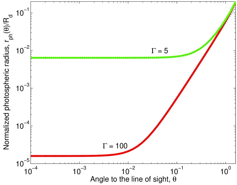
Figure 1.— Normalized photospheric radius $r_{ph}(\theta)/R_{d}$ as a function of the angle to the line of sight, $\theta$. The thick lines show the exact solution of equation 3 for $\Gamma=100$ (lower line) and $\Gamma=5$ (upper line). The dotted lines show the approximate solution $r_{ph}/R_{d}=(\theta^{2}/3+\Gamma^{-2})/2\pi$. The approximate result in equation 4 is nearly identical to the exact solution for $\theta\leq 1$.

2.1. Characteristic time scale for observation of thermal emission in GRBs

The strong angular dependence of the photospheric radius (equation 4), implies that thermal photons originating from high angles to the line of sight can be observed on a very long time scale following the decay of the inner engine that produces the thermal emission. Below the photosphere, the photons are coupled to the flow, therefore their velocity component in the direction of the flow is $\approx\beta c$. Assuming that a photon is emitted at $t=0$, $r=0$, it emerges from the photosphere at time $t=r_{ph}(\theta)/\beta c$. Photons that propagate towards the observer at angle to the line of sight $\theta$ are thus observed at a time delay compared to a hypothetical photon that was emitted at $t=0$, $r=0$ and did not suffer any time delay (“trigger” photon), which is given by $\Delta t^{ob.}(\theta)=[r_{ph}(\theta)/\beta c]\times[1-\beta\cos(\theta)]$.

For relativistic outflows, $\Gamma\gg 1$, photons emitted on the line of sight ($\theta=0$) are thus seen at a time delay with respect to the trigger photon,

$$\Delta t^{ob.}(\theta=0)\simeq{R_{d}\over 4\pi\Gamma^{4}\beta c}\simeq 10^{-2}L_{52}\Gamma_{2}^{-5}\,\rm{s}.$$ (5)

Here, ${\dot{M}}=L/\Gamma c^{2}$, and typical parameters characterizing GRBs, $L=10^{52}L_{52}{\rm\,ergs^{-1}}$ and $\Gamma=100\Gamma_{2}$ were used.

Photons emitted from high angles to the line of sight, $\theta\gg\Gamma^{-1}$ (and $\theta\ll 1$) are observed at a much longer time delay,

$$t^{ob.}(\theta\gg\Gamma^{-1})\simeq{R_{d}\over 3\pi\beta c}\left({\theta^{2}\over 2}\right)^{2}\simeq 30\,L_{52}\Gamma_{2}^{-1}\theta_{-1}^{4}{\rm\,s},$$ (6)

where $\theta=0.1\theta_{-1}$. The time scale derived on the right hand side of equation 6 is based on the estimate of the jet opening angle in GRB outflow, $\theta\leq\theta_{j}\simeq 0.1$ (e.g., Berger et al. , 2003). One can thus conclude, that in relativistically expanding wind with parameters characterizing emission from GRBs, thermal emission can be observed up to tens of seconds following the decay of the inner engine.

3. Photon energy loss due to the slight misalignment of the scattering electrons velocity vectors below the photosphere

Below the photosphere, photons undergo repeated Compton scattering with the electrons in the flow. For a jet with finite, constant opening angle, the velocity vectors of the electrons propagating inside the jet are slightly misaligned. This, in turn, leads to photon energy loss via repeated Compton scattering as the photons propagate downstream. This mechanism is independent on the adiabatic energy losses of the electrons, and thus dominates if the electrons comoving temperature decreases faster than $r^{-2/3}$ (see below).

In order to calculate the photon energy loss, I assume that the comoving electrons temperature can be neglected, and take the limit $T^{\prime}_{el}=0$. Consider a single scattering event between a photon and an electron inside the flow. I explicitly assume that the photon energy in the (local) comoving frame is low, $\varepsilon^{\prime}\ll m_{e}c^{2}$. In the scattering event, the photon is being scattered to angle $\theta^{\prime}$, in the (local) comoving frame. Denoting by $\varepsilon^{\prime}$ the photon energy before the scattering (the incoming photon energy), its outgoing energy is given by $\varepsilon_{1}^{\prime}=\varepsilon^{\prime}\left\{1+(\varepsilon^{\prime}/m_{e}c^{2})\times[1-\cos(\theta^{\prime})]\right\}^{-1}\simeq\varepsilon^{\prime}$. Thus, the photon local comoving energy is not changed by a single scattering event.

Consider two consequent scattering events, the first of which occurs at radius $r_{i}$ and the second at radius $r_{i+1}$. Due to the symmetry in the scattering direction, on the average the photon propagation direction is parallel to the flow. Assuming that before the first scattering the photon propagation direction is parallel to the velocity vector of the first scatterer electron, following the first scattering event, the photon propagation direction is at angle $\theta_{\gamma}$ with respect to the first electron velocity vector (in the lab frame), where $\cos(\theta_{\gamma})=[\beta+\cos(\theta^{\prime})]/[1+\beta\cos(\theta^{\prime})]$. After being scattered, the photon travels a distance $\Delta r_{i}$ until it is being scattered again. The velocity vector of the consequent scatterer electron makes an angle $\theta_{el}$ with the velocity vector of the first electron (see figure 2). The two electrons assume to propagate at a similar Lorentz factor, $\Gamma$. As discussed above, the photon comoving energy in the rest frame of the first scatterer, $\varepsilon^{\prime}_{i}$ is unchanged by the scattering process. However, Lorentz transformation to the rest frame of the consequent scatterer implies that the photon comoving energy in this frame is given by

$$\begin{array}[]{lcl}\varepsilon_{i+1}^{\prime}&=&\varepsilon_{i}^{\prime}{\Big{\{}}\Gamma^{2}\left[1-\beta^{2}\cos(\theta_{el})\right]\\ &&\quad\;-\Gamma^{2}\beta\left[\cos(\theta_{el})-1\right]{\left[\cos(\theta_{\gamma})-\beta\right]\over 1-\beta\cos(\theta_{\gamma})}\\ &&\quad\;\left.-\Gamma\beta\sin(\theta_{el}){\sin(\theta_{\gamma})\over\Gamma\left[1-\beta\cos(\theta_{\gamma})\right]}\right\}.\end{array}$$

The photon scattering angle $\theta_{\gamma}$ and the angle between the two electrons velocity vectors, $\theta_{el}$ are related via

$$\tan(\theta_{el})={\Delta r_{i}\sin(\theta_{\gamma})\over r_{i}+\Delta r_{i}\cos(\theta_{\gamma})}$$ (7)

(see figure 2).

Equation 3 can be considerably simplified by noting that in the lab frame the photon scattering angle $\theta_{\gamma}\sim\Gamma^{-1}\ll 1$, and that below the photosphere the average distance traveled by the photon between consequent scattering is small, $\Delta r_{i}/r_{i}\ll 1$ (see below). Thus, one can approximate $\tan(\theta_{el})\approx\theta_{el}\approx(\Delta r_{i}/r_{i})\sin(\theta_{\gamma})$ and $\cos(\theta_{el})\approx 1-\theta_{el}^{2}/2$. With these approximations, equation 3 becomes

$$\begin{array}[]{lcl}\varepsilon_{i+1}^{\prime}&\simeq\varepsilon_{i}^{\prime}&\Big{\{}1+{\Gamma^{2}\beta^{2}\over 2}\left({\Delta r_{i}\over r_{i}}\right)^{2}\sin^{2}(\theta_{\gamma})\\ &&\quad+{\Gamma^{2}\beta\over 2}\left({\Delta r_{i}\over r_{i}}\right)^{2}{\sin^{2}(\theta_{\gamma})\left[\cos(\theta_{\gamma})-\beta\right]\over 1-\beta\cos(\theta_{\gamma})}\\ &&\quad\left.-\beta\left({\Delta r_{i}\over r_{i}}\right){\sin^{2}(\theta_{\gamma})\over 1-\beta\cos(\theta_{\gamma})}\right\}.\end{array}$$

Of the three terms in the right hand side of equation 3 that contribute to the energy change between consequent scatterings, the last term is the dominant. Using $\sin(\theta_{\gamma})\sim\Gamma^{-1}={\mathcal{O}}(\Gamma^{-1})$, one finds that $1-\beta\cos(\theta_{\gamma})={\mathcal{O}}(\Gamma^{-2})$, and $\cos(\theta_{\gamma})-\beta={\mathcal{O}}(\Gamma^{-2})$. Therefore, the first two terms are of the order of $(\Delta r_{i}/r_{i})^{2}$, while the last term is of the order of $(\Delta r_{i}/r_{i})$. Thus, for $(\Delta r_{i}/r_{i})\ll 1$, equation 3 is approximated as

$$\varepsilon_{i+1}^{\prime}\approx\varepsilon_{i}^{\prime}\left[1-\beta\left({\Delta r_{i}\over r_{i}}\right){\sin^{2}(\theta_{\gamma})\over 1-\beta\cos(\theta_{\gamma})}\right].$$ (8)

Figure 2.— Schematic view of two consequent scattering geometry in the lab (observer) frame.

In order to determine the energy loss of a photon it is thus required to estimate the ratio $(\Delta r_{i}/r_{i})$. Calculation of this ratio is done by transforming to the cylindrical coordinate system presented in §2, in which the $z$ axis is the photon propagation direction. The first of the two considered scattering occurs at location $z_{\min}$ along this axis, and the proceeding scattering occurs at location $z_{\max}$. Under these definitions, $\Delta r_{i}=z_{\max}-z_{\min}$. The small scattering angle (in the lab frame) implies that $\theta_{\gamma}\approx\tan(\theta_{\gamma})=r_{\min}/z_{\min}$, and that the radii of the consequent scatterings can be approximated as $r_{i}\simeq z_{\min}$, $r_{i+1}\simeq z_{\max}$ (see figure 2).

Using these approximation in equation 3, one finds that the optical depth at the first scattering point is $\tau_{i}\approx(R_{d}/2\pi z_{\min})\times[\Gamma^{-2}+(r_{\min}/z_{\min})^{2}/3]$, and at the consequent scattering point it is $\tau_{i+1}\approx(R_{d}/2\pi z_{\max})\times[\Gamma^{-2}+(r_{\min}/z_{\max})^{2}/3]$. Writing the optical depth between consequent scattering as $\Delta\tau_{i}=\tau_{i}-\tau_{i+1}$ thus leads to

$$\Delta\tau_{i}={R_{d}\over 2\pi\Gamma^{2}}\left({1\over z_{\min}}-{1\over z_{\max}}\right)+r_{\min}^{2}{R_{d}\over 6\pi}\left({1\over z_{\min}^{3}}-{1\over z_{\max}^{3}}\right).$$ (9)

Equation 9 can be simplified using $\Delta r_{i}=z_{\max}-z_{\min}$ and the assumption $\Delta r_{i}\ll r_{i}$,

$$\Delta\tau_{i}\simeq\Delta r_{i}{R_{d}\over 2\pi z_{\min}^{2}}\left({1\over\Gamma^{2}}+{r_{\min}^{2}\over z_{\min}^{2}}\right)\approx\Delta r_{i}{R_{d}\over 2\pi r_{i}^{2}}\left({1\over\Gamma^{2}}+\theta_{\gamma}^{2}\right).$$ (10)

Since, on the average $\langle\Delta\tau_{i}\rangle=1$, one obtains

$$\langle\Delta r_{i}\rangle={r_{i}^{2}\over{R_{d}\over 2\pi}\left({1\over\Gamma^{2}}+\theta_{\gamma}^{2}\right)}.$$ (11)

Comparison with equation 3 shows that equation 11 justifies the assumption $\Delta r_{i}/r_{i}\ll 1$ used so far, as long as the photon propagation occurs in region of high optical depths. Using further this assumption in equations 8 and 11, the (local) photon comoving energy and radius after $n$ scattering events can be approximated as

$$\begin{array}[]{lcl}\varepsilon_{n}^{\prime}&\approx&\varepsilon_{1}^{\prime}e^{-nr_{1}\langle\omega\rangle};\\ r_{n}&\approx&r_{1}e^{nr_{1}\langle\alpha\rangle}.\end{array}$$

Here, $\varepsilon_{1}^{\prime}$, $r_{1}$ are the photon comoving energy and radius at the point in which the photon is introduced into the plasma, $\langle\omega\rangle$ and $\langle\alpha\rangle$ are the average of the functions

$$\begin{array}[]{lcl}\langle\omega\rangle&=&{\bigg{\langle}}{\beta\sin^{2}(\theta_{\gamma})\over{R_{d}\over 2\pi}\left({1\over\Gamma^{2}}+\theta_{\gamma}^{2}\right)[1-\beta\cos(\theta_{\gamma})]}{\bigg{\rangle}};\vskip 3.0pt plus 1.0pt minus 1.0pt\\ \langle\alpha\rangle&=&{\bigg{\langle}}{1\over{R_{d}\over 2\pi}\left({1\over\Gamma^{2}}+\theta_{\gamma}^{2}\right)}{\bigg{\rangle}}\end{array}$$

over the scattering events angles. Note that both $\omega$ and $\alpha$ are functions only of the photon scattering angle, $\theta_{\gamma}$ (for constant flow parameters, $R_{d}$ and $\Gamma$, as assumed here).

Equation 3 implies that the comoving energy of photons decreases with radius as

$$\varepsilon^{\prime}(r)\propto r^{-{\langle\omega\rangle\over\langle\alpha\rangle}}.$$ (12)

The values of the functions $\langle\omega\rangle$ and $\langle\alpha\rangle$ are calculated in §4.2 below.

4. Late time decay of the observed temperature and flux of the thermal emission

As long as the radiative processes that produce the thermal photons deep inside the flow are active, the observed thermal radiation is dominated by photons emitted on the line of sight towards the observer. Once these radiative processes are terminated, the radiation becomes dominated by photons emitted off axis and from larger radii on a very short time scale (see eq. 5). In order to calculate the observed thermal flux and temperature at late times, it is thus required to calculate the probability of a photon to be emitted from radius $r$ and angle to the line of sight $\theta$. Since thermal photons are coupled to the flow below the photosphere, the emission radius of these photons is in fact the radius in which the last scattering event takes place.

In the calculation below, I assume that photons are coupled to the flow via Compton scattering below the last scattering event radius, $r$. Below this radius, the photons velocity vector is, on the average, parallel to the direction of the flow. At the last scattering event, the photon is being scattered into angle $\theta$ with respect to the direction of the flow. Since below $r$ the velocity component of the photon in the direction of the flow is $\approx\beta c$, a photon emitted at time $t=0$ decouples from the plasma at time $t_{dcp}\simeq r/\beta c$. This photon is observed at a delay with respect to the “trigger” photon that was emitted at $t=0$, $r=0$ and propagates towards the observer by $t^{ob.}\equiv\Delta t^{ob.}=r/{\beta c}\times[1-\beta\cos(\theta)]\equiv ru/{\beta c}$. Denoting by $T^{\prime}(r)$ the comoving temperature of the photons at radius $r$, the observed temperature of the photons is $T^{ob.}=T^{\prime}(r){\mathcal{D}}$, where ${\mathcal{D}}=[\Gamma(1-\beta\mu)]^{-1}$ is the Doppler factor, and $\mu\equiv\cos(\theta)$. The observed flux and temperature are thus functions of $r$ and $\theta$ (or $u$).

The calculation of the photospheric radius presented in §2 gives, by definition, the radius above which the optical depth to scattering is equal to unity. Photons, however, have a finite probability of being scattered at any point in space in which electrons exist. Thus, the calculation presented in §2 needs to be extended to include the finite probability of photons to be emitted at any radius and into arbitrary angle. I introduce here calculation of this probability density function $P(r,\theta)$ under some simplified approximations, which allow full analytic calculation of the flux and temperature at late times. The results of an exact numerical calculation are presented in §5 below. It is shown there that the analytical calculations presented here are in very good agreement with the exact numerical results.

4.1. Probability of photons to decouple from the plasma at radius $r$ and be scattered into angle $\theta$

The increase of the photospheric radius with the angle to the line of sight, $\theta$ (see eq. 4) implies that the probability of a photon to be scattered at angle $\theta$ is $r$-dependent. Nonetheless, as suggested by the numerical results in §5 below, this dependence is limited to a cutoff at a maximum angle from which photons are observed $\theta_{\max}(r)$, and does not affect much the probability of photons to be scattered to smaller angles, $\theta<\theta_{\max}$. In the model below, I thus make a separation of variables to write $P(r,\theta)=P(r)\times P(\theta)$. The validity of this assumption (as well as the other approximations used) is verified by the numerical results presented in §5.

The probability of the last scattering event of a thermal photon to occur at radius $r..r+\delta r$ is calculated in the following way. The optical depth $\tau(r,\theta)$ for a photon scattered at radius $r$ into angle $\theta$ to reach the observer was calculated in equation 3. In determining the probability of a photon to be scattered from radius $r..r+\delta r$, the angle into which the scattering occurs is of no importance . One can therefore write the dependence of the optical depth on the radius as $\tau(r)\propto r^{-1}$ (see eq. 3). This optical depth is the integral over the scattering probability of a photon propagating from radius $r$ to $+\infty$, i.e., $\tau(r)=\int_{r}^{\infty}(d\tau/dr)dr$, from which it is readily found that $(d\tau/dr)|_{r}\propto r^{-2}$. As the photon propagates from radius $r$ to $r+\delta r$, the optical depth in the plasma changes by $\delta\tau=(d\tau/dr)|_{r}\delta r$. Therefore, the probability of a photon to be scattered as it propagates from radius $r$ to $r+\delta r$ is given by

$$P_{sc.}(r..r+\delta r)=1-e^{-\delta\tau}\approx\delta\tau\propto{\delta r\over r^{2}}.$$ (13)

For the last scattering event to take place at $r..r+\delta r$, it is required that the photon will not undergo any additional scattering before it reaches the observer. The probability that no additional scattering occurs from radius $r$ to the observer is given by $\exp(-\tau[r])$. The probability density function $P(r)$ for the last scattering event to occur at radius $r$, is therefore written as

$$P(r)={r_{0}\over r^{2}}e^{-(r_{0}/r)}.$$ (14)

The function $P(r)$ in equation 14 is normalized, $\int_{0}^{\infty}P(r)dr=1$. By comparison to equation 3, the proportionality constant is $r_{0}\equiv r_{ph}(\theta=0)=R_{d}/2\pi\Gamma^{2}$.

The probability of a photon to be scattered into angle $\theta$ is calculated as follows. Since photons undergo multiple Compton scattering below the photosphere, I assume that before the last scattering event the photon propagation direction is parallel to the flow. In the following, I neglect the dipole approximation in the last scattering event angle, $\theta^{\prime}$. I thus assume that in the local comoving frame the scattering is isotropic, i.e., $d\sigma/d\Omega^{\prime}=Const$. This approximation was checked numerically to be valid (see §5 below). Since the spatial angle $d\Omega^{\prime}=\sin\theta^{\prime}d\theta^{\prime}d\phi^{\prime}$, the probability of a photon to be scattered to angle $\theta^{\prime}$ (in the comoving frame) is $dP/d\theta^{\prime}\propto\sin\theta^{\prime}$. Integrating over the range $0\leq\theta^{\prime}\leq\pi$ gives the normalization factor $1/2$. Thus, the isotropic scattering approximation leads to $P(\theta^{\prime})=(\sin\theta^{\prime})/2$.

Using Lorentz transformation to the observer frame, the probability of scattering into angle $\theta$ with respect to the flow direction, which is the observed angle to the line of sight is

$$\begin{array}[]{lcl}P(\theta)&=&P(\theta^{\prime}){d\theta^{\prime}\over d\cos\theta^{\prime}}{d\cos\theta^{\prime}\over d\cos\theta}{d\cos\theta\over d\theta}\vskip 3.0pt plus 1.0pt minus 1.0pt\\ &=&{\sin\theta\over 2\Gamma^{2}(1-\beta\cos\theta)^{2}}.\end{array}$$

Using the definition $u\equiv 1-\beta\cos\theta$, equation 4.1 becomes

$$P(u)={1\over 2\Gamma^{2}\beta u^{2}}.$$ (15)

Note that $1-\beta\leq u\leq 1+\beta$, and the function $P(u)$ in equation 15 is normalized, $\int_{1-\beta}^{1+\beta}P(u)du=1$.

4.2. Temporal evolution of the observed flux and temperature at late times

The diffusion model presented above implies that thermal photons emerging from the expanding plasma (i.e., last scattered) at radius $r$ and into angle $\theta$ are observed at time $t^{ob.}=ru/\beta c$. This assumption implies that all the photons are introduced into the plasma (by radiative processes occurring deep inside the flow) at the same instance, i.e., the photon injection function is assumed to be a $\delta$-function in time. For finite photon injection function, the result is a convolution of the $\delta$-function calculation presented here. For a quick termination of the inner engine, the $\delta$-function approximation leads to a good description of the temporal evolution of temperature and flux at late times, once the inner engine terminates.

Following the decay of the inner engine, the observed flux at time $t^{ob.}$ is proportional to the probability of photon emission from radius $r$ and into angle $\theta$ by

$$\begin{array}[]{lcl}F(t^{ob.})&=&F_{0}\int_{r_{\min}}^{r_{\max}}P(r)dr\int_{u_{\min}}^{u_{\max}}P(u)du\times\delta\left(t^{ob.}={ru\over\beta c}\right)\\ &=&F_{0}\int_{r_{\min}}^{r_{\max}}{r_{0}\over r^{2}}e^{-(r_{0}/r)}dr\int_{1-\beta}^{1+\beta}{1\over 2\Gamma^{2}\beta u^{2}}du\\ &&\times\left({\beta c\over r}\right)\delta\left(u={\beta ct^{ob.}\over r}\right)\\ &=&F_{0}{r_{0}\over 2\Gamma^{2}\beta^{2}c{t^{ob.}}^{2}}\left[E_{1}(z_{\min})-E_{1}(z_{\max})\right].\end{array}$$

At a given observed time $t^{ob.}$, the integration boundaries are $r_{\max}=\beta ct^{ob.}/u_{\min}=\Gamma^{2}\beta ct^{ob.}/(1+\beta)$, and $r_{\min}=\beta ct^{ob.}/(1+\beta)$. In evaluating the integral in the second line, I use $z\equiv r_{0}/r$, which lead to $z_{\max}=(1+\beta)r_{0}/(\beta ct^{ob.})$ and $z_{\min}=(1-\beta)r_{0}/(\beta ct^{ob.})$. These can be written with the use of normalized time, $t_{N}\equiv r_{0}(1-\beta)/c$ as $z_{\max}=[(1+\beta)/(1-\beta)](t_{N}/\beta t^{ob.})$ and $z_{\min}=t_{N}/\beta t^{ob.}$. In the final formula, $E_{1}(z)\equiv\int_{z}^{\infty}e^{-t}t^{-1}dt$ is the exponential integral.

At late times, $t^{ob.}\gg t_{N}$, the difference of the two exponential integrals can be written as $E_{1}(z_{\min})-E_{1}(z_{\max})\approx\log(z_{\max}/z_{\min})$, which enables to write the temporal decay of the observed flux as

$$F(t^{ob.})\approx F_{0}{r_{0}\over 2\Gamma^{2}\beta^{2}c{t^{ob.}}^{2}}\log\left({1+\beta\over 1-\beta}\right).$$ (16)

I thus find that the thermal flux decays at late times as $F(t^{ob.})\propto{t^{ob.}}^{-2}$.

In order to calculate the temporal change in the observed temperature, the power law index of the photons comoving energy decay with radius, resulting from the misalignment of the velocity vectors of the electrons below the photosphere needs to be specified. The average values of the functions $\langle\omega\rangle$ and $\langle\alpha\rangle$ (eq. 3) are determined with the use of the probability density function $P(u)$ given in equation 15. By doing so, I assume that the conditions that led to the validity of equation 15 for the last scattering event (i.e., that before the scattering the photon propagation direction is parallel to the flow, and the neglection of the dipole approximation) hold for every scattering below and close to the photosphere. I further use the fact that $\Gamma\gg 1$ and the average photon scattering angle below the photosphere $\langle\theta_{\gamma}\rangle\ll 1$ to approximate $u=1-\beta\cos\theta_{\gamma}\simeq(\theta_{\gamma}^{2}/2+1/2\Gamma^{2})$, and $\sin\theta_{\gamma}\simeq\theta_{\gamma}$. Using these approximations in equation 3, one obtains

$$\begin{array}[]{lcl}\langle\omega\rangle&\simeq&{\bigg{\langle}}{\beta\theta_{\gamma}^{2}\over{2R_{d}\over 2\pi}u^{2}}{\bigg{\rangle}}\simeq{\bigg{\langle}}{2\beta\over{2R_{d}\over 2\pi}u}-{\beta\over{2R_{d}\over 2\pi}\Gamma^{2}u^{2}}{\bigg{\rangle}};\vskip 3.0pt plus 1.0pt minus 1.0pt\\ \langle\alpha\rangle&\simeq&{\bigg{\langle}}{1\over{2R_{d}\over 2\pi}u}{\bigg{\rangle}}.\end{array}$$

The mean of the functions $\langle u^{-1}\rangle$, $\langle u^{-2}\rangle$ is calculated using equation 15,

$$\begin{array}[]{lcl}\langle u^{-1}\rangle&=&\int_{1-\beta}^{1+\beta}{P(u)\over u}du=\Gamma^{2};\vskip 3.0pt plus 1.0pt minus 1.0pt\\ \langle u^{-2}\rangle&=&{\Gamma^{4}\over 3}(3+\beta^{2})\simeq{4\over 3}\Gamma^{4}.\end{array}$$

Using equation 4.2, it is readily found that $\langle\omega\rangle\simeq(1/3)\beta\Gamma^{2}/(R_{d}/2\pi)$, and $\langle\alpha\rangle\simeq(1/2)\Gamma^{2}/(R_{d}/2\pi)$. Using these results in equation 12 leads to the conclusion that the comoving photon energy decays with radius as

$$\varepsilon^{\prime}(r)\propto r^{-{2\beta\over 3}}\simeq r^{-2/3}.$$ (17)

The arguments leading to equation 17, in particular the requirement $\Delta r_{i}/r_{i}\ll 1$ are valid below the photosphere (see §3 , eq. 11). Therefore, at radii much larger than $r_{0}$ a deviation from this law is expected. Comparison with the numerical results (§5, figure 5 below) shows that indeed at large radii $r\gg r_{0}$ the photon comoving energy becomes $r$ independent. This result can be understood since above the photosphere the optical depth is smaller than unity, and, if a photon is being scattered at all then the number of scattering it undergoes is no more than one or two at most. In calculating the observed temperature at late times, I thus assume that the comoving photon energy decreases with radius as $\varepsilon^{\prime}(r)\propto r^{-2/3}$ at $r\leq A_{brk}\times r_{0}$, and $\varepsilon^{\prime}(r)\propto r^{0}$ at larger radii, where $A_{brk}=few$.

The photons spectral distribution is thermal, resulting from thermalization processes occurring in regions deep inside the flow, which are characterized by very high optical depth. As the photons propagate outwards, their energy decreases, however the thermal spectrum is unchanged (see further discussion in §6 below). At any given instance, an observer sees photons emitted from a range of radii and angles. Therefore, even if the comoving energy spectrum of the photons is thermal (black body), the observed spectrum deviates from black body, and is a grey body. Nonetheless, being a convolution of black body spectra, the observed spectrum is not expected to deviate much from black body spectra. The effective temperature of the observed spectra is

$$T^{ob.}(t^{ob.})=\frac{\int_{r_{\min}}^{r_{\max}}P(r)dr\int_{u_{\min}}^{u_{\max}}P(u)duT^{ob.}(r,u)\delta\left(t^{ob.}={ru\over\beta c}\right)}{\int_{r_{\min}}^{r_{\max}}P(r)dr\int_{u_{\min}}^{u_{\max}}P(u)du\delta\left(t^{ob.}={ru\over\beta c}\right)},$$ (18)

where $T^{ob.}(r,u)=T^{\prime}(r){\mathcal{D}}=T^{\prime}(r)/\Gamma u$, and

$$T^{\prime}(r)=\left\{\begin{array}[]{ll}T^{\prime}_{0}\left({r\over{\bar{r}}}\right)^{-2/3}&r\leq A_{brk}r_{0},\\ T^{\prime}_{0}\left({A_{brk}r_{0}\over{\bar{r}}}\right)^{-2/3}&r>A_{brk}r_{0}.\end{array}\right.$$

In evaluating the numerator in equation 18, one needs to discriminate between two cases. At early times, $t^{ob.}<A_{brk}t_{N}/\beta$, $r_{\max}<A_{brk}r_{0}$, and therefore the break in the comoving temperature occurs at radius which is outside the integration boundaries. At these times, equation 18 becomes

$$\begin{array}[]{lcl}T^{ob.}(t^{ob.};t^{ob.}\leq A_{brk}t_{N})&=&{T^{\prime}_{0}\over\Gamma}{{\bar{r}}^{2/3}\over\beta ct^{ob.}}\frac{\int_{r_{\min}}^{r_{\max}}{r_{0}\over r^{2/3}}e^{-(r_{0}/r)}dr}{\int_{r_{\min}}^{r_{\max}}{r_{0}\over r}e^{-(r_{0}/r)}dr}\\ &=&{T^{\prime}_{0}\over\Gamma}{{\bar{r}}^{2/3}r_{0}^{1/3}\over\beta ct^{ob.}}\Gamma\left(-{1\over 3}\right)\vskip 3.0pt plus 1.0pt minus 1.0pt\\ &&\times\frac{\left[P\left(-{1\over 3},z_{\max}\right)-P\left(-{1\over 3},z_{\min}\right)\right]}{E_{1}(z_{\min})-E_{1}(z_{\max})}.\end{array}$$

Here, $P(a,z)\equiv[1/\Gamma(a)]\int_{0}^{z}e^{-t}t^{a-1}dt$ is incomplete Gamma function. At early enough times, $t^{ob.}\ll t_{N}$, $z_{\max}\gg z_{\min}\gg 1$. Equation 4.2 can be put in a simpler form by expanding the exponential integrals $E_{1}(z)\simeq e^{-z}/z$ and the incomplete Gamma function, $\Gamma(-1/3)P(-1/3,z)\simeq-e^{-z}/z^{4/3}$. With these approximations, equation 4.2 becomes

$$\begin{array}[]{lcl}T^{ob.}(t^{ob.};t^{ob.}\leq A_{brk}t_{N})&\simeq&{T^{\prime}_{0}\over\Gamma}{{\bar{r}}^{2/3}r_{0}^{1/3}\over\beta ct^{ob.}z_{\min}^{1/3}}\vskip 3.0pt plus 1.0pt minus 1.0pt\\ &=&{T^{\prime}_{0}{\bar{r}}^{2/3}(1+\beta)^{1/3}\over\Gamma^{1/3}(\beta ct^{ob.})^{2/3}}.\end{array}$$

At later observed times $t^{ob.}>A_{brk}t_{N}/\beta$, the break in the comoving temperature occurs at radius which is inside the integration boundaries. Splitting the integral over $r$ in the numerator of equation 18 into two, one obtains

$$\begin{array}[]{lcl}T^{ob.}(t^{ob.};t^{ob.}\geq A_{brk}t_{N})&=&{T^{\prime}_{0}\over\Gamma}{{\bar{r}}^{2/3}r_{0}^{1/3}\over\beta ct^{ob.}}\\ &&\vskip 3.0pt plus 1.0pt minus 1.0pt\times\frac{I_{1}+I_{2}}{E_{1}(z_{\min})-E_{1}(z_{\max})},\end{array}$$

where

$$\begin{array}[]{lcl}I_{1}&=&\Gamma\left(-{1\over 3}\right)\left[P\left(-{1\over 3},z_{\max}\right)-P\left(-{1\over 3},{1\over A_{brk}}\right)\right],\\ I_{2}&=&A_{brk}^{-2/3}\left[{e^{-z_{\min}}\over z_{\min}}-A_{brk}e^{-1/A_{brk}}\right.\\ &&\qquad\qquad+E_{1}(A_{brk}^{-1})-E_{1}(z_{\min})\Big{]}.\end{array}$$

Unfortunately, for the relevant time scale $t^{ob.}/t_{N}\lesssim 10^{4}$, (see §5) there is no simpler analytic approximation to equation 4.2.

5. Numerical calculation of the flux and temperature decay at late times

The analytical calculations presented above were checked with a numerical code. The code is a Monte-Carlo simulation, based on earlier code developed for the study of photon propagation in relativistically expanding plasma (Pe’er & Waxman, 2004; Pe’er et al. , 2006b). I give below a short description of the numerical code, before presenting the numerical results and a comparison to the analytical approximations developed above.

5.1. The numerical model

I consider a three-dimensional plasma wind expanding from an initial radius $r_{i}$ that fills the entire volume $r>r_{i}$. Following the standard dynamics of GRB outflow (e.g., Mészáros & Rees, 2000), the plasma assumed to accelerate up to the saturation radius $r_{s}=\Gamma r_{i}$, above which it expands at constant Lorentz factor, $\Gamma$. The plasma is assumed to be ejected at a time independent rate, $\dot{M}=L/\Gamma c^{2}$, where $L$ is the (observed) luminosity. Therefore, the plasma comoving density decreases with radius above $r_{s}$ as $n^{\prime}(r)=\dot{M}/(4m_{p}\Gamma\beta cr^{2})$. Since below $r_{s}$, $\Gamma(r)\propto r$, considering adiabatic energy losses the plasma comoving temperature at $r\geq r_{s}$ is given by

$$\begin{array}[]{lcl}T^{\prime}_{el}(r)&=&{k_{B}\over\Gamma m_{e}c^{2}}\left({L\over 4\pi r_{i}^{2}ca}\right)^{1/4}\left({r\over r_{s}}\right)^{-2/3}\vskip 3.0pt plus 1.0pt minus 1.0pt\\ &=&7.3\times 10^{-3}\,L_{52}^{1/4}r_{i,8}^{1/6}\Gamma_{2}^{-1/3}r_{10}^{-2/3}.\end{array}$$

Here, $T^{\prime}_{el}$ is given in normalized units of $m_{e}c^{2}$ and the convention $Q=10^{x}Q_{x}$ is adopted in cgs units.

Photons are injected into the plasma in a random position on the surface of a sphere at radius $r_{inj}=R_{d}/(2\pi\Gamma^{2}d)$. The depth $d$ is taken as $d=20$ in order to ensure that the probability of a photon to escape without being scattered is smaller than $\exp(-20)$, i.e., negligible. The initial photon propagation direction is random, and its (local) comoving energy at the injection radius is equal to the plasma comoving temperature at this radius.

Given the position of the scattering event and the photon 4-vector, the position of the next scattering event is calculated as follows. The code transforms the scattering position into the cylindrical coordinate system presented in §2, in which the scattering position is ($r_{\min},z_{\min}$). Using $\theta=\tan^{-1}(r_{\min}/z_{\min})$, the code calculates the optical depth for the photon to escape, using equation 3. It then draws an optical depth $\Delta\tau$ from a logarithmic distribution, which represents the optical depth traveled by the photon until the next scattering event. If $\Delta\tau$ is larger than the optical depth to escape, the photon assumes to escape, and the time difference between this photon and a hypothetical photon that propagated parallel to the last propagation direction of the photon and was not scattered is calculated.

If $\Delta\tau$ is smaller than the optical depth to escape, the next scattering position is calculated along the photon propagation direction, i.e., it occurs in position ($r_{\min},z_{\max}$). $z_{\max}$ is calculated such that the difference in optical depths between the initial scattering point and the next scattering point is equal to $\Delta\tau$. The scattering position is then transformed back to the standard Cartesian coordinates.

Given the scattering position, the electrons temperature is drawn from a Maxwellian distribution with temperature given by equation 5.1. The photon 4-vector is Lorentz transformed twice: first into the (local) frame of the bulk motion of the flow, which assumed to move at constant Lorentz factor $\Gamma$ in the radial direction. Second, transformation into the electrons rest frame (the electron assumed to move randomly within the bulk motion frame). The photon interact with the electrons via Compton scattering. The full Klein-Nishina cross section is considered in the interaction, in which the scattered angles of the outgoing photon are drawn. The outgoing photon energy and its new propagation direction are calculated in the electrons’ rest frame. The program then Lorentz transforms the photon 4-vector back into the lab (Cartesian) frame, and repeats the calculation until the photon escapes.

5.2. Numerical results

The position of the last scattering events for $N=10^{5}$ simulated photon propagation inside the expanding plasma is presented in figure 3. The last scattering event points are shown in the $r-\theta$ plane, on top of the photospheric radius calculated in equations 3 and 4. In preparing the plot, parameters characterizing GRBs (see eq. 5.1) were taken. In the figure, the last scattering event radius is normalized to $r_{0}=R_{d}/2\pi\Gamma^{2}$. Therefore, results obtained for arbitrary values of the free model parameters ($L$ and $\Gamma$) that characterize astrophysical transients other than GRBs, such as AGNs or microquasars are similar to the ones presented. Clearly, the photospheric radius calculated in equation 4 gives a first order approximation of the last scattering events radii and angles. However, it is obvious from the figure that photons decouple from the plasma at a range of radii and angles, necessitating the use of the probability density functions calculated in §4.

The normalized observed flux is presented in figure 4, together with the analytical result in equation 4.2. In producing this figure, the photons are assumed to be injected as a $\delta$-function in time. As the photons propagate outwards, the program traces the time in which every scattering event occurs. Once the photon propagation direction after the last scattering event is known, calculation of the observed time is done by calculating the lag of the particular photon with respect to a hypothetical (“trigger”) photon that propagated in a direction parallel to the final propagation direction of the photon, and did not undergo any scatterings.

Physical transient sources emit during a finite time duration. Since the photon injection function is assumed here to be a $\delta$ function in time, it is clear that the results presented are valid for late time emission only, after the central engine that produced the photon emission had decayed. The early time rise in the flux is thus expected to deviate from the results presented here, and depend on the properties of the emission mechanism in physical transients. The late time power law decay, $F(t^{ob.})\propto{t^{ob.}}^{-2}$ is a prediction of the model. The time scale in figure 4 is presented in normalized units of $t_{N}$, and thus is useful for any transient sources.

For parameters characterizing GRBs, $t_{N}\simeq 10^{-2}\,L_{52}\Gamma_{2}^{-5}$ s. Since, as calculated above (see §2.1, eq. 6), thermal emission from GRBs is expected to last tens of seconds, the relevant time scale is $t/t_{N}\approx 10^{4}$. It is shown in figure 4 that on this time scale the approximation in equations 4.2, 16 are in excellent agreement with the numerical results. This fact confirms the validity of the approximations introduced in the analytical calculations in §4.

The numerical results show that at very early times, $t/t_{N}<10^{-1}$, the analytical result presented in equation 4.2 does not predict the high flux expected. This indicates the limitations of the model, in particular the assumption that the observed time depends only on two parameters, the last scattering event radius and angle. As the photons diffuse below the photosphere, inevitably there is a small spreading in their arrival times to radius $r$, which is not considered in the analytical calculations. This discrepancy, however, is limited to very short time scales, in which, as discussed above, the actual nature of the inner engine activity determines the observed flux.

The (local) comoving photon energy at the last scattering event radius is presented in figure 5. It is shown that indeed for $r<r_{0}$, $\varepsilon^{\prime}(r)\propto r^{-2/3}$, as calculated in equation 17. This justifies the approximations that led to that equation. At larger radii, the approximations that led to equation 17 no longer hold, as the number of scattering a photon undergo above this radius is no more than a few. As a result, the photon comoving energy becomes $r$-independent.

The decay law index of the electrons comoving temperature in equation 5.1, $2/3$, is similar to the decay law index of the photon temperature calculated in §3. In order to check that the mechanism described in §3 is indeed independent on the decay law index of the electrons comoving temperature, additional runs with decay law index larger than $2/3$ were performed. The results obtained in these runs were similar to the results presented in figure 5.

The observed temperature as a function of time is presented in figure 6. The numerical results are shown by the blue solid line, and the analytical approximation calculated in equations 4.2 and 4.2 are presented by the red dashed line. In preparing the plots, $A_{brk}=3$ was taken, in accordance to the numerical results of the comoving energy decay at large radii (see figure 5). Clearly, the analytical formula gives a good approximation to the numerical results, although the numerical results show that the power law decay of the temperature is somewhat steeper than the analytical approximation at late times: $T^{ob.}(t^{ob.})\propto{t^{ob.}}^{-\beta}$, with $\beta\simeq 2/3$ at $t/t_{N}\lesssim 30$ becoming $\beta\approx 1/2$ at later times. The model presented here thus predicts a late time power law decay of the observed temperature, with power law index $\beta$ that slightly decreases over a time scale of $\sim 100t_{N}$ from $\beta\simeq 2/3$ to $\beta\approx 1/2$. For parameters characterizing GRBs, this time scale corresponds to few seconds.

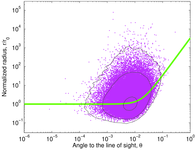
Figure 3.— Position of the last scattering event point in $\theta$-$r$ plane for $10^{5}$ events. The solid (green) line is the photospheric radius, calculated in equation 4. Clearly, the last scattering events take place in a range of radii and angles. The photospheric radius gives a first order approximation to the position of these events. The contour lines are added to the plot in order to indicate the density of the emerging photons radii and angles.

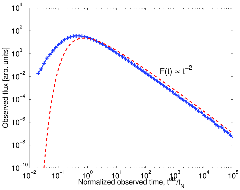
Figure 4.— Observed thermal flux as a function of the observed time. The solid (blue) line is the numerical simulation result, and the dash (red) line is the analytic approximation in equation 4.2. Time is given in units of normalized time, $t_{N}$. For $t/t_{N}\gtrsim 1$, the thermal flux decays as $F(t^{ob.})\propto{t^{ob.}}^{-2}$

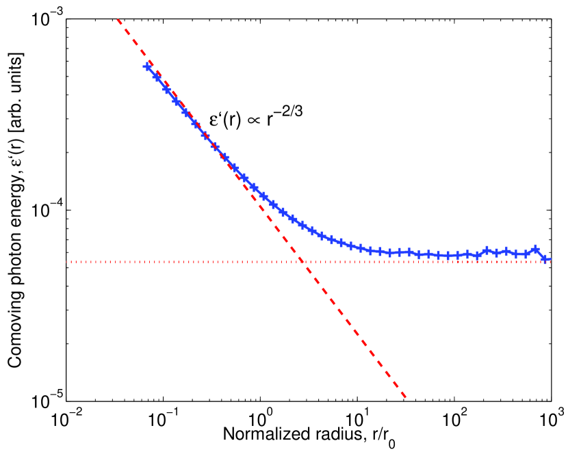
Figure 5.— Photon (local) comoving energy as a function of radius, at the last scattering event radius. Numerical results are presented by the solid (blue) line. The results indicate that for $r/r_{0}<1$, $\varepsilon^{\prime}(r)\propto r^{-2/3}$, in accordance with the results of equation 17. At larger radii, the arguments leading to the result in equation 17 no longer hold, and the photon (local) comoving energy becomes $r$-independent.

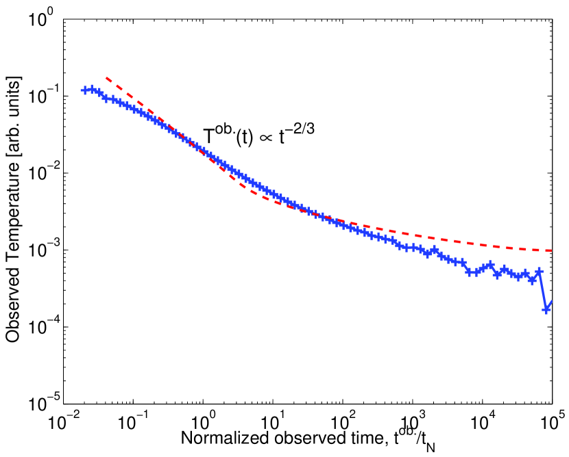
Figure 6.— Observed temperature as a function of the observed time. The solid (blue) line is the numerical simulation results, and the dash (red) line is the analytic approximation in equations 4.2 and 4.2, with $A_{brk}=3$. The numerical results are slightly smoother than the analytical approximation. The temperature decays as a power law in time, with power law index $\beta\simeq 2/3$ at $t/t_{N}\lesssim 10$, and $\beta\approx 1/2$ at later times.

6. Summary and discussion

In this paper, I addressed the question of late time thermal emission from optically thick, relativistically expanding plasma winds. I first showed in §2 that the photospheric radius depends on the angle to the line of sight, $\theta$ in a non-trivial way: for $\theta<\Gamma^{-1}$, $r_{ph}$ is $\theta$-independent, while for $\theta>\Gamma^{-1}$, $r_{ph}(\theta)\propto\theta^{2}$ (eq. 4). I used this result in §2.1 to show that for parameters characterizing emission from GRBs, thermal emission can be seen up to tens of seconds following the decay of the inner engine (eq. 6). In §3 I showed that photons lose their energy due to repeated Compton scattering below the photosphere. The mechanism responsible for this energy loss is based on the geometrical effect of the misalignment between the velocity vectors of the electrons in the expanding plasma jet. This mechanism is therefore unrelated to other mechanisms discussed so far in the literature (e.g., adiabatic expansion, or the mechanism leading to Kompaneets equation). I showed that as a result of this mechanism, the (local) comoving temperature of the photons decreases below the photosphere as $\varepsilon^{\prime}(r)\propto r^{-2/3}$ (eq. 17). I introduced in §4 the probability density function $P(r,\theta)=P(r)\times P(\theta)$ that extend the definition of a photosphere to include the actual positions and angles in space from which thermal photons decouple from the plasma. Using these functions, I calculated the temporal decay of the observed flux (eqs. 4.2, 16) and temperature (eqs. 4.2, 4.2) of the thermal emission, and showed that both decay as a power law in time, following the decay of the inner engine that produces the thermal photons. The flux decays as $F(t^{ob.})\propto{t^{ob.}}^{-\alpha}$ with $\alpha=2$, and the temperature decays as $T(t^{ob.})\propto{t^{ob.}}^{-\beta}$ with $\beta=2/3$ at early times which later changes to $\beta\simeq 1/2$. The analytical results were confirmed with the results of the numerical simulation presented in §5.

The results presented here can account for the recent observations of thermal emission that accompanies long duration GRBs. As was shown by Ryde (2004, 2005), after $\sim 1-3$ s the temperature of the thermal component decreases as a power law in time, $T^{ob.}\propto t^{-\alpha}$, with power law index $\alpha\simeq 0.6-1.1$. An additional analysis (F. Ryde & A.Pe’er 2008, in preparation) shows that after a short rise, the flux of the black body component of these bursts also decreases with time as $F_{BB}^{ob.}\propto t^{-\beta}$, with power law index $\beta\approx 2.0-2.5$. These results are thus naturally reproduced by the model presented here.

A key consequence of the model presented here is that thermal emission at early times (before the observed break) is dominated by thermal photons originating from the photosphere on the line of sight. Therefore, observation of the thermal emission at early times, when the inner engine is still active, gives a direct measurement of the temperature and flux of photons emitted from the photospheric radius on the line of sight, $r_{0}\equiv r_{ph}(\theta=0)$. This is the innermost radius from which information can reach the observer.

The interpretation presented here has a direct implication in the study of relativistic outflows. For GRBs with known redshift, early time (before the break) observation of the temperature and flux of the thermal component enabled direct determination of two of the least restricted parameters of the fireball model: the bulk motion Lorentz factor, $\Gamma$ and the radius at the base of the flow (Pe’er et al. , 2007). Being based on thermal emission only, the method presented in this paper is insensitive to many of the inherent uncertainties in former methods of determining the values of these parameters. Future measurements with the upcoming GLAST satellite will enable to increase the sample of GRBs with known redshift from which thermal emission component is identified, to further test the model presented here and to gain statistics on the values of the fireball model parameters.

In addition to the prompt emission phase in GRBs, thermal activity may occur as part of the flaring activity observed in the early afterglow phase of many GRBs (Burrows et al. , 2005; Falcone et al. , 2007). The exact nature of these flares is currently not yet clear. As it is plausible that the flares result from renewed emission from the inner core, a renewed thermal emission may occur. Analyzing this emission in a method similar to the one described here and by Pe’er et al.  (2007), may thus provide information on the flow parameters during the late time flaring activity.

The relevance of the results obtained here is not limited only to emission from GRBs, but also to emission from any transient phenomenon characterized by relativistic outflow, such as AGNs and microquasars. Provided there is a source of photons deep inside the flow, following the decay of this source the decay laws of the thermal flux and temperature derived above hold for any such object. An important point here, is that the nature of the mechanism that produces the radiation is of no importance, as long as it occurs deep inside the flow so that the photons thermalize before they escape.

In this work, I assumed that the electrons are cold (in the comoving frame), and that the electrons and photons interact only via Compton scattering. If this is not the case, due, e.g., to some dissipation mechanism that produces energetic electrons at different regions of the flow, than Compton scattering with energetic electrons will lead to modification of the thermal spectrum. This case was extensively studied by Rees & Mészáros (2005); Pe’er et al.  (2005, 2006). As was shown in these works, the thermal photons in this case serve as seed photons to Compton scattering that produces high energy, non-thermal spectrum. However, if the optical depth in which the energetic electrons are introduced into the flow is smaller than $\sim$ unity, then the thermal component can be separated from the non-thermal one (Pe’er et al. , 2006). Note that this is exactly the case in the internal collision model of GRBs: internal shocks can only occur at radii larger than the spreading radius, $r_{spread}=\Gamma r_{S}=10^{12}\,r_{i,8}\Gamma_{2}^{2}$ cm, which is similar to $r_{0}=6\times 10^{12}\,L_{52}\Gamma_{2}^{-3}$ cm. Thus, the optical depth in the region where internal shocks can occur is not expected to exceed a few. I can thus conclude that thermal emission is expected to be observed in GRBs under the assumptions of the internal collisions model.

The late time thermal emission predicted here essentially arises from emission off the line of sight. It is thus similar in nature to the high latitude emission discussed in the literature, in the context of GRB afterglow emission (Fenimore, Madras & Nayakshin, 1996; Woods & Loeb, 1999; Kumar & Panaitescu, 2000). All these works, however, treated the optically thin case, which is relevant for the afterglow emission phase from GRBs. The work presented here differs by treating thermal emission from optically thick plasmas, characterizing the very early stages of emission from GRBs.

One of the key findings in this work is the new mechanism in which photons lose their energy below the photosphere. This mechanism differs than other mechanisms discussed in the literature so far for radiative cooling below the photosphere. The result obtained, $\varepsilon^{\prime}(r)\propto r^{-2/3}$ holds for relativistic jets characterized by constant ($r$-independent) jet opening angle. For jets in which the jet opening angle is $r$-dependent, a different power law decay in the photon energy is expected.

In the calculation of the photon energy loss presented in §3, I neglected the electrons temperature. As the photons propagate downstream, their comoving temperature cannot be lower than the comoving temperature of the electrons. The electrons temperature decreases due to adiabatic expansion, which result in a decay of the electrons temperature as a power law in the comoving plasma volume, $T^{\prime}_{el}\propto{V^{\prime}}^{-1/3}$ (for relativistic electrons). Adopting the fireball model of GRBs (for review, see, e.g. Mészáros, 2006), above the saturation and below the spreading radii of the fireball, the comoving volume is $V^{\prime}\propto r^{2}$, resulting in a decrease of the comoving electrons temperature as $T^{\prime}_{el}(r)\propto r^{-2/3}$. Above the spreading radius, the comoving volume increases as $V^{\prime}\propto r^{3}$, which implies $T^{\prime}_{el}(r)\propto r^{-1}$. In any of these regimes, the electrons temperature decreases with the radius at least as fast as the photon temperature.

The mechanism presented here for photon energy loss has some resemblance to adiabatic energy losses, as the photon temperature is converted into work done on the electrons. However, it is a different mechanism having a different origin. Adiabatic energy losses occur once the plasma expands, and its volume increases. As opposed to that, in the scenario considered here, the volume in which photons interact with the electrons (the volume below the photosphere) does not expand, since for constant flow parameters (${\dot{M}},\Gamma$) the photospheric radius is time independent. In addition, as discussed above, the decay law of the photon energy is independent on the electrons temperature (as long as the electrons comoving temperature is not higher than the photon comoving temperature). The fact that between the saturation radius and the spreading radius in GRBs the decay law of the photons and electrons comoving temperature is similar, is thus a coincidence.

References

- Abramowicz et al. (1991) Abramowicz M.A., Novikov, I.D., & Paczyński, B. 1991, ApJ, 369, 175
- Berger et al. (2003) Berger, E., Kulkarni, S.R., & Frail, D. 2003, ApJ, 590, 379
- Burrows et al. (2005) Burrows, D.N., et al. 2005, Science, 309, 1833
- Dermer (2004) Dermer, C.D. 2004, ApJ, 614, 284
- Falcone et al. (2007) Falcone, A.D., et al. 2007, ApJ, 671, 1921
- Fenimore, Madras & Nayakshin (1996) Fenimore, E.E., Madras, C.D., & Nayakshin, S. 1996, ApJ, 473, 998
- Goodman (1986) Goodman, J. 1986, ApJ, 308, L43
- Gopal-Krishna et al. (2006) Gopal-Krishna, et al. 2006, MNRAS, 377, 446
- Hjellming & Rupen (1995) Hjellming, R.M., & Rupen, M.P. 1995, Nature, 375, 464
- Kumar & Panaitescu (2000) Kumar, P., & Panaitescu, A. 2000, ApJ, 541, L51
- Lind & Blandford (1985) Lind, K.R., & Blandford, R.D. 1985, ApJ, 295, 358
- Mészáros (2006) Mészáros, P. 2006, Rep. Prog. Phys., 69, 2259
- Mészáros & Rees (2000) Mészáros, P., & Rees, M.J. 2000, ApJ, 530, 292
- Mirabel & Rodriguez (1994) Mirabel, I.F., & Rodriguez, L.F. 1994, Nature, 371, 46
- Paczyński (1986) Paczyński, B. 1986, ApJ, 308, L43
- Paczyński (1990) Paczyński, B. 1990, ApJ, 363, 218
- Pe’er et al. (2005) Pe’er, A., Mészáros, P., & Rees, M.J. 2005, ApJ, 635, 476
- Pe’er et al. (2006) Pe’er, A., Mészáros, P., & Rees, M.J. 2006, ApJ, 642, 995
- Pe’er et al. (2006b) Pe’er, A., Mészáros, P., & Rees, M.J. 2006, ApJ, 652, 482
- Pe’er et al. (2007) Pe’er, A., Ryde, F., Wijers, R.A.M.J., Mészáros, P., & Rees, M.J. 2007, ApJ, 664, L1
- Pe’er & Waxman (2004) Pe’er, A., & Waxman, E. 2004, ApJ, 613, 448
- Rees & Mészáros (2005) Rees, M.J., & Mészáros, P. 2005, ApJ, 628, 847
- Ryde (2004) Ryde, F. 2004, ApJ, 614, 827
- Ryde (2005) Ryde, F. 2005, ApJ, 625, L95
- Ryde & Petrosian (2002) Ryde, F., & Petrosian, V. 2002, ApJ, 578, 290
- Woods & Loeb (1999) Woods, E., & Loeb, A. 1999, ApJ, 523, 187