Families of spatial solitons in a two-channel waveguide with the cubic-quintic nonlinearity

Abstract

We present eight types of spatial optical solitons which are possible in a model of a planar waveguide that includes a dual-channel trapping structure and competing (cubic-quintic) nonlinearity. Among the families of trapped beams are symmetric and antisymmetric solitons of “broad” and “narrow” types, composite states, built as combinations of broad and narrow beams with identical or opposite signs (“unipolar” and “bipolar” states, respectively), and “single-sided” broad and narrow beams trapped, essentially, in a single channel. The stability of the families is investigated via eigenvalues of small perturbations, and is verified in direct simulations. Three species – narrow symmetric, broad antisymmetric, and unipolar composite states – are unstable to perturbations with real eigenvalues, while the other five families are stable. The unstable states do not decay, but, instead, spontaneously transform themselves into persistent breathers, which, in some cases, demonstrate dynamical symmetry breaking and chaotic internal oscillations. A noteworthy feature is a stability exchange between the broad and narrow antisymmetric states: in the limit when the two channels merge into one, the former species becomes stable, while the latter one loses its stability. Different branches of the stationary states are linked by four bifurcations, which take different forms in the model with the strong and weak inter-channel coupling.

I Introduction and the model

Self-trapping of light beams in the form of spatial solitons in planar waveguides, which was demonstrated experimentally about two decades ago spatial-soliton , is one of fundamental effects in nonlinear optics . The variety of the spatial solitons may be greatly expanded if the waveguide is equipped with a multi-channel structure Wang , that can be created by a permanent transverse modulation of the refractive index, or induced, in a photorefractive crystal, by a pair of laser beams (with the ordinary polarization) illuminating the crystal in transverse directions, while the probe beam, that creates the soliton(s), is launched in the extraordinary polarization Moti . Besides their interest to optical physics, manipulations of spatial solitons by means of multi-channel trapping structures have a vast potential for applications to routing of data streams Wang .

The transmission of the electromagnetic wave with local amplitude $\psi(z,x)$ along axis $z$ in the multi-channel planar waveguide is modeled by the nonlinear Schrödinger (NLS) equation. In the normalized form, the equation is

$$i\psi_{z}+\psi_{xx}-V(x)\psi+\delta n\left(|\psi|^{2}\right)\psi=0,$$ (1)

where the second term accounts for the transverse diffraction, $V(x)$ represents the transverse modulation of the refractive index that induces the multi-channel structure, and term $\sim\delta n(|\psi|^{2})$ represents the optical nonlinearity, $\delta n\left(|\psi|^{2}\right)=n_{2}|\psi|^{2}$, with $n_{2}>0$, corresponding to the ordinary Kerr effect. In the model including the Kerr term and simplest transverse modulation, $V(x)=V_{0}\cos\left(2\pi x/L\right)$, solitons trapped in channels and a possibility of switching them between the channels were studied in Ref. Wang . It was found that the entire family of fundamental (single-humped) solitons, with any value of integral power, $P=\int_{-\infty}^{+\infty}|\psi(x)|^{2}dx$, is stable. A family of stable double-humped bound states of fundamental solitons exists in this model too, provided that the power exceeds a certain threshold value which grows with the increase of $V_{0}$. A possibility of the switching, realized as carrying the fundamental soliton over into an adjacent channel, was also shown in Ref. Wang , under the action of a local kick (“hot spot”), represented by an additional term $\sim\delta(x-x_{0})\delta(z-z_{0})\psi$ in Eq. (1), where $x_{0}$ is a midpoint between the channels.

The same model as the one introduced in Ref. Wang , but with $z$ replaced by time $t$ was later considered as an effectively one-dimensional Gross-Pitaevskii equation for the Bose-Einstein condensate (BEC) trapped in the optical-lattice potential KonotopEPL (the general topic of condensates trapped in optical lattices was reviewed in Refs. BEC-OL-reviews ). In the model with the sinusoidal transverse modulation replaced by that of the Kronig-Penney (KP) type, i.e., a periodic array of rectangular potential troughs, soliton states were studied in Ref. Smerzi , and an effective nonlinear band structure in the same model was analyzed in detail in Refs. Carr . The KP structure is quite relevant for applications to optics, where it corresponds to the simplest step-index profile of the transverse modulation.

In addition to employing the multichannel settings, the variety of spatial-soliton states can be greatly expanded by using media with competing self-focusing and self-defocusing nonlinearities. A well-known example of that is provided by the cubic-quintic (CQ) nonlinearity. Optical nonlinearities of the CQ type were observed in chalcogenide glasses glass , and in some organic materials organic . Actually, the CQ nonlinear response of these media is induced by an intrinsic resonance, which also gives rise to nonlinear (two-photon) absorption Leblond . Nevertheless, according to analysis reported in Ref. YiFan , effects of the loss may be neglected in physically relevant settings, as experiments in optical crystals are conducted over sufficiently short propagation distances (a few centimeters) spatial-soliton ; Moti . It is also relevant to mention that the CQ nonlinearity was predicted Agarwal and recently observed Brazil in composite optical media (colloids).

Equation (1) with the CQ nonlinearity can be cast into the following normalized form we ; we-all :

$$i\psi_{z}+\psi_{xx}=V(x)\psi-2|\psi|^{2}\psi+|\psi|^{4}\psi.$$ (2)

In the uniform medium, which corresponds to $V(x)=0$, Eq. (2) gives rise to the well-known family of stable solitons Canada ,

$$\psi_{\mathrm{sol}}(x,z)=e^{ikz}\sqrt{\frac{2k}{1+\sqrt{1-4k/3}\cosh\left(2\sqrt{k}x\right)}},$$ (3)

which is parameterized by propagation constant $k$ which takes values in interval

$$0<k<k_{\max}\equiv 3/4.$$ (4)

In an adjacent interval, $3/4\leq k\leq 1$, solutions exist too, in the form of continuous-wave (CW) states with a constant amplitude,

$$\psi_{\mathrm{CW}}^{(\pm)}(z)=e^{ikz}\sqrt{1\pm\sqrt{1-k}}$$ (5)

(the CW solutions exist for all $k\leq 1$). The total power of soliton (3) is

$$P_{\mathrm{sol}}(k)=\frac{\sqrt{3}}{2}\ln\left(\frac{\sqrt{3}+2\sqrt{k}}{\sqrt{3}-2\sqrt{k}}\right).$$ (6)

CW solution (5) with the larger amplitude, $\psi_{\mathrm{CW}}^{(+)}$, are stable, while solutions $\psi_{\mathrm{CW}}^{(-)}$ are subject to the modulational instability. At $k=1$, both branches of the CW solutions merge and disappear through the ordinary tangent bifurcation JosephIooss . Note that the width of soliton (3) diverges as

$$W\approx\left(1/\sqrt{3}\right)\left|\ln\left(k_{\max}-k\right)\right|$$ (7)

in the limit of $k\rightarrow k_{\max}=3/4$, see Eq. (4), and, accordingly, the soliton asymptotically goes over into the stable CW state, $\psi_{\mathrm{CW}}^{(+)}$, in this limit. In terms of the bifurcation theory, the disappearance of the bright soliton at this point is explained by its merger with a dark-soliton solution to Eq. (2) with $V=0$, which also exists at $k<k_{\max}\equiv 3/4$. Exactly at $k=3/4$, the dark soliton degenerates into a front solution, which vanishes in one limit, at $x\rightarrow\pm\infty$, and asymptotically coincides with the CW state in the other,

$$\psi_{\mathrm{front}}(x,z)=e^{\left(3/4\right)iz}\sqrt{\frac{3/2}{1+e^{\pm\sqrt{3}x}}}~{}.$$ (8)

A natural possibility, which is promising both for the exploration of fundamental properties of guided solitons and for potential applications, is to study localized states generated as a result of the interplay between the CQ nonlinearity and multichannel waveguiding structures. In Ref. we , solitons were investigated in the CQ model including a single guiding channel of a rectangular shape. A distinctive feature of the channel-trapped solitons in that model is their bistability: while in interval (4), which hosts solution family (3) in the free space, the channel supports a single soliton state for each $k$, the full existence region of the solitons includes an additional interval, $3/4<k<\tilde{k}_{\max}$ (the value of $\tilde{k}_{\max}$ depends on the depth and width of the guiding channel), where two different solitons are found for a given value of $k$, both being stable (note that a guiding channel does not give rise to soliton bistability in the model with the cubic nonlinearity gh ).

The combination of the CQ nonlinearity with a periodic array of guiding channels of the KP type was studied in Ref. we-all . In addition to single-humped (fundamental) solitons, many families of stable multi-humped (higher-order) solutions, which also feature the bistability, were found in that model. Independently, a model combining the CQ nonlinearity and a periodic sinusoidal modulation function was introduced in Ref. China , where similar results for soliton families were obtained. Note that both these versions of the model including the CQ terms and periodic potential function $V(x)$ generate not only soliton families in the semi-infinite spectral gap, but also solitons in finite bandgaps, provided that the potential is strong enough. The finite-gap solitons are stable too, but they do not feature bistability.

The most relevant setting for applications to the all-optical switching is based on two parallel guiding channels, rather than a periodic array. The respective model is based on Eq. (2) with the effective potential in the form of

$$V(x)=\left\{\begin{array}[]{ll}0,&|x|~{}<L/2~{}\mathrm{and~{}}|x|~{}>D+L/2,\\ -V_{0},&L/2<|x|~{}<D+L/2,\end{array}\right.$$ (9)

where $V_{0}$, $D$ and $L$ are, respectively, the depth and width of each channel, and the thickness of the barrier which separates them. This model is also interesting in terms of the soliton dynamics, as it opens a way to study spontaneous symmetry breaking (SSB) in spatial solitons supported by the two-channel configuration. The SSB in settings based on double potential wells has recently drawn a great deal of interest in the studies of BEC, where it was realized experimentally Markus , and analyzed theoretically, using, chiefly, finite-mode approximations, that replace the underlying Gross-Pitaevskii equation by a system of ordinary differential equations finite-mode . A conclusion produced by the analysis is that double-well systems with the self-attractive cubic nonlinearity (self-focusing, in terms of optics) give rise to stable asymmetric states (which is known as “macroscopic quantum self-trapping”) through destabilization of symmetric states, while the systems with the self-repulsive (defocusing) nonlinearity feature destabilization of antisymmetric solutions. The latter mechanism also generates stable asymmetric states.

Actually, a similar finite-mode analysis of the SSB of CW states in a nonlinear optical coupler (which, for this purpose, is essentially tantamount to the double-channel waveguide) was published much earlier in Ref. Canberra . That work reported results for the model with the self-focusing or defocusing Kerr nonlinearity, as well as for a saturable nonlinearity. SSB in a double-well optical setting has been implemented in a photorefractive crystal (which corresponds to the saturable nonlinearity) Zhigang .

The objective of the present work is to find symmetric, antisymmetric and asymmetric self-trapped states (i.e., spatial solitons, in terms of nonlinear optics) in the two-channel model with the CQ nonlinearity, based on Eqs. (2) and (9), and explore bifurcations linking those states to each other. An obvious difference from the previous works, both those relying upon the finite-mode approximation finite-mode and works which analyzed the full two-channel configuration in the combination with the cubic nonlinearity, such as Ref. Michal , is the competition between the self-focusing and self-defocusing nonlinearities, which drastically alters various states, their stability, and bifurcations.

Note that dynamical switching of nonlinear localized beams in the same model as considered here was investigated in a recent work Radik , by means of a variational approximation and direct simulations. The analysis had revealed four different transmission regimes, depending on the total power of the beam. However, stationary states were not looked for in that work.

The rest of the paper is organized as follows. In Sec. II, we present basic types of stationary spatial solitons which are possible in the model, and analyze their stability in Sec. III. Depending on the symmetry and width of the solitons, we identify eight types of the states, five stable and three unstable (in the same configuration with the cubic nonlinearity, only three soliton species exist). The stability of each species is established in a rigorous form, via the computation of eigenvalues for modes of small perturbations around the solitons, and verified in direct simulations. For all unstable solutions, the instability eigenvalues are real. However, in direct simulations the instability does not destroy the trapped states, but rather transforms them into robust breathers, that may feature dynamical SSB, and chaotic intrinsic oscillations, in some cases. In Sec. IV, we demonstrate generic families (branches) of different soliton species, and bifurcations that link them together. The bifurcation diagrams are essentially different in cases of the strong and weak coupling between the two channels, i.e., roughly speaking, for small and large values of separation $L$ between them, see Eq. (9). The solution branches and bifurcation diagrams are displayed in two different forms, viz., as the total power versus the propagation constant, cf. Eq. (6), and also as an effective asymmetry parameter of the state (it is defined below as  per Eq. (13)) versus the total power. The paper is concluded by Sec. V.

II Basic types of spatial solitons in the two-channel system

In the model with the CQ nonlinearity, each waveguiding channel can support localized states of two different types, which we will call narrow and broad ones. The “narrow” state is nothing else but soliton (3) trapped in the channel, while its “broad” counterpart may be realized as a trapped fragment of CW state (5). In fact, the bistability of soliton states found in the CQ model with the single channel we is accounted by the coexistence of stable solutions of these two types. In the two-channel system, these states may be combined in different ways. First, symmetric and antisymmetric spatial solitons, each built of narrow (Fig. 1) or broad (Fig. 2) beams trapped in each channel, is easily found as a numerical solution of the equation obtained from Eq. (2) by the substitution of $\psi(z,x)=\exp\left(ikz\right)u(x)$ with real function $u(x)$,

$$u^{\prime\prime}=ku+V(x)u-2u^{3}+u^{5}.$$ (10)

Numerical solution of Eq. (10) was performed by means of the relaxation method based on the Newton-Raphson algorithm (formally speaking, this equation with $V(x)$ taken in the form given by Eq. (9) can be solved analytically, as explicit solutions in terms of elliptic functions are available in each region where $V(x)$ takes a constant value; however, the continuity conditions for $u(x)$ and $u^{\prime}(x)$ at points $|x|=L/2$ and $|x|=D+L/2$ give rise to very cumbersome transcendental equations).

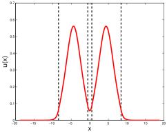
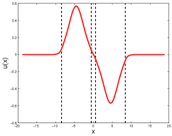
Figure 1: (Color online) Typical examples of symmetric (a) and antisymmetric (b) spatial solitons built of narrow beams trapped in the two channels. These examples and those displayed below for other generic types of spatial solitons in the two-channel system are displayed for the two-channel potential (9) with $V_{0}=3$, $D=8$, $L=1$, and propagation constant $k=3.25$, see Eq. (10). Borders of the trapping channels are shown (here and in other figures) by vertical dashed lined.

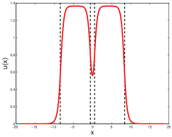
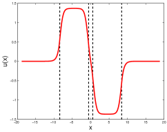
Figure 2: (Color online) Typical examples of symmetric (a) and antisymmetric (b) spatial solitons formed by broad pulses trapped in the two channels. Parameters are the same as in Fig. 1.

As mentioned above, the NLS equation with the CQ nonlinearity in the free space, i.e., Eq. (2) with $V(x)=0$, admits not only exact solutions in the form of the bright solitons and CW states, as given by Eqs. (3) and (5), but also dark-soliton solutions. Accordingly, the antisymmetric bound states of two broad beams, a generic example of which is displayed in Fig. 2(b), may be realized as a “curtailed” dark soliton (the one whose flat background was chopped off) trapped in the two-channel setting.

Further, using a broad beam placed in one channel, and its narrow counterpart in the other, it is easy to find solutions to Eq. (10) in the form of asymmetric composite states, as shown in Fig. 3. The composite states, as well as the bistability of spatial solitons trapped in a single channel we , are specific features of the model with the CQ nonlinearity (one may expect the same features in models with more general competing nonlinearities), which are not supported by nonlinearities of non-competing types, such as those represented by cubic or saturable terms in the NLS equation. The signs of the two components of the composite spatial solitons may be identical or opposite, see Figs. 3(a) and 3(b). We will refer to these two species as unipolar and bipolar composite solitons, respectively.

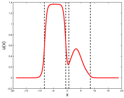
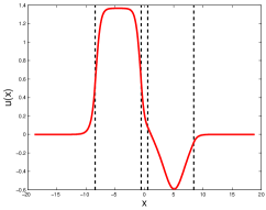
Figure 3: (Color online) Typical examples of unipolar (a) and bipolar (b) asymmetric spatial solitons built as bound states of broad and narrow pulses trapped in the two channels. Parameters are the same as in Fig. 1.

Asymmetric states that, as said above, are well known in models combining double-well potentials and cubic or saturable nonlinearity finite-mode -Michal , have their straightforward counterparts in the present model, in the form of a narrow or broad beam trapped in one channel, while the other channel is left almost empty. Typical examples of these (strongly asymmetric) states, which are different from the above-mentioned moderately asymmetric composite spatial solitons, are displayed in Fig. 4. Below, we refer to them as “single-sided” states.

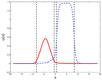
Figure 4: (Color online) Generic examples of the single-sided states, with one channel carrying a narrow or broad pulse (they are shown, respectively, by solid and dashed curves in the left and right parts of the figure), while the other channel is nearly empty. Parameters are the same as in Fig. 1.

A noteworthy feature of the single-sided broad-beam solution is that, for $k$ approaching the maximum value, $k_{\max}=3/4$, above which soliton (3) cannot exist in the free space, according to Eqs. (4) and (7), and is replaced by the spatially infinite CW state, $\psi_{\mathrm{CW}}^{(+)}$ (see Eq. (5)), the broad-beam solution goes over not into something close to $\psi_{\mathrm{CW}}^{(+)}$, but, instead, into a front state which is similar to exact solution (8), as shown in Fig. 5. Recall that, in the free space, the front solution exists at a single value of the propagation constant, $k=3/4$, while an external potential may support a family of front solutions DW (in Ref. DW , fronts were represented by solutions to the Gross-Pitaevskii equation which included the cubic nonlinearity and a sinusoidal potential). In the present model, it can be shown that front states may also be sustained by a single potential well, in the absence of the second channel. We note that such a solution (which is stable, see below) was not reported in the previous analysis of the single-channel CQ model we .

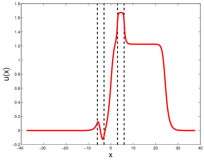
Figure 5: (Color online) An example of a stable single-sided broad beam, which is very close to the transition into a front-shaped state. Parameters of the two-channel potential are $V_{0}=3$, $D=3$, $L=6$, and the propagation constant is extremely close to value $k_{\max}=3/4$ which corresponds to the transition between the dark-soliton and CW states, via front configuration (8), in the free space (see Eq. (4)), $k=0.75+10^{-16}$.

Examples of the eight different species of spatial solitons possible in the present model (symmetric and antisymmetric narrow and broad states, unipolar and bipolar composite ones, and broad or narrow single-sided solutions) were shown in Figs. 1-4 for a set of parameters at which the coupling between the channels is relatively strong (this is seen in the lack of strong separation between two components of the solitons in Figs. 1(a), 2(a), and 3(a)). In the limit of $L\rightarrow 0$, when the buffer layer that separates the channels disappears, and we thus return to the single-channel setting, the symmetric states continuously go over into single-humped solitons (narrow or broad ones), which were studied in Ref. we . In the same limit, the antisymmetric states gradually turn into a dipole (soliton-antisoliton pair) trapped in the remaining single channel. These transitions are illustrated by Fig. 6, which shows the total power of each symmetric and antisymmetric soliton family, $P$, versus $L$ – from $L=0$, that corresponds to a single channel of width $2D$, up to large values of $L$, that correspond to isolated channels of width $D$. Note that the power of the narrow symmetric state in the limit of large $L$, i.e., the total power of the set of two fundamental solitons, is naturally very close to $2P(L=0)$, since the power at $L=0$ is that of a single soliton. On the other hand, it is natural too that powers of the broad states trapped in the single channel of the double width (at $L=0$), and in two widely separated channels (at larger $L$) are nearly equal, as, for the nearly-CW configurations, $P$ is proportional to the total width of the area filled by the wave.

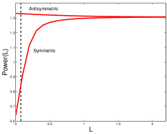
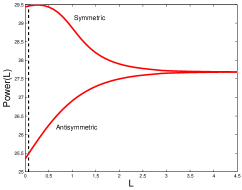
Figure 6: (Color online) The total power of the antisymmetric and symmetric narrow (a) and broad (b) solitons as a function of thickness $L$ of the buffer layer between the channels. Fixed parameters are $V_{0}=3$, $D=8$, and $k=3.1$. The dashed vertical lines mark small values of $L$ at which the stability is switched, see text.

Unlike the symmetric and antisymmetric states, the evolution of asymmetric ones, i.e., the trapped beams of the unipolar and bipolar composite and single-sided types, with the decrease of $L$ is not continuous. It was found that, at some small critical value of $L$, each asymmetric state performs a jump, either into a symmetric state (unipolar composite and single-sided spatial solitons), or into an antisymmetric one (the bipolar composite spatial soliton).

Examples of antisymmetric states found in the limit of $L=0$ in the single channel are displayed in Fig. 7. Such dipole states were not considered in the framework of the previous work dealing with spatial solitons in the single-channel CQ model we . However, they are qualitatively similar to the so-called “dark-in-the-bright” solitons that were investigated as solutions to the Gross-Pitaevskii equation with a parabolic confining potential Yannis . The peculiarity of the model with the CQ nonlinearity is that it provides for the coexistence of two different trapped dipoles at a common value of $k$, similar to the bistability of the trapped fundamental solitons. A noteworthy finding is that the stability of narrow and broad antisymmetric solitons trapped in a single channel is opposite to that of their counterparts in the two-channel setting, where the families of narrow and broad antisymmetric states are, respectively, stable and unstable (see below): in the single channel, the narrow dipole is unstable, while the broad one is stable. In fact, the stability switch occurs at very small finite values of $L$, which are marked by dashed vertical lines in Fig. 6.

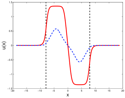
Figure 7: (Color online) An example of antisymmetric spatial solitons (dipoles), narrow and broad ones (shown by the dashed and solid curves, respectively), trapped in the single channel of width $2D$ (edges of the channel are marked by dashed vertical lines). Parameters are $V_{0}=3$, $2D=16$, and $k=3.1$. The narrow dipole is unstable, while its broad counterpart is stable.

In addition to the states trapped in the channels, we have also found solutions for beams trapped in the buffer layer between the channels. Such settings are known as nonlinear antiwaveguides gh ; Gisin . We do not display those solutions here because, as may be naturally expected, they are subject to a strong instability.

III Stability of the spatial solitons

Stability of the eight families of spatial solitons found in the two-channel setting was investigated in two complementary ways, viz., by numerical computation of stability eigenvalues from linearized equations for small perturbations, and by means of direct simulations of perturbed solitons. Both methods have produced identical conclusions concerning the stability or instability of each family of the stationary states.

For the analysis of small perturbations, the solution was looked for as

$$\psi(x,z)=e^{ikz}\left[u(x)+\epsilon\left(U(x)\exp\left(\sigma z\right)+V^{\ast}(x\right)\exp\left(\sigma^{\ast}z\right)\right],$$ (11)

where $u(x)$ is a real stationary solution pertaining to propagation constant $k$, the asterisk stands for the complex conjugation, $\epsilon$ is a real infinitesimal amplitude of the perturbation with complex eigenmodes $U(x)$ and $V(x)$, that are associated to a (generally, complex) eigenvalue $\sigma$. As usual, the stability condition is $\mathrm{Re}(\sigma)=0$, which must hold for all the eigenvalues. The substitution of expression (11) in Eq. (2) and linearization yield the eigenvalue problem that can be written a matrix form,

$$\left(\begin{array}[]{cc}\hat{L}+i\sigma&2u^{2}(x)\left[1-u^{2}(x)\right]\\ 2u^{2}(x)\left[1-u^{2}(x)\right]&\hat{L}-i\sigma\end{array}\right)\left(\begin{array}[]{c}U\\ V\end{array}\right)=0,$$ (12)

where the Sturm-Liouville operator is $\hat{L}\equiv d^{2}/dx^{2}-V(x)+u^{2}(x)\left[4-3u^{2}(x)\right]-k$. Numerical analysis of the stability spectrum was performed by the computation of eigenvalues of a large-size matrix approximating the operator on the left-hand side of Eq. (12).

The following results have been obtained. Five species of the spatial solitons are stable in entire domains of their existence (i.e., all the respective stability eigenvalues have zero real parts, up to the accuracy of the numerical computation), with the exception of the above-mentioned stability switch of the antisymmetric states at very small values of $L$. Thus, the following families of stable solutions can be identified:

(i) Narrow antisymmetric states, an example of which is displayed above in Fig. 1(b).

(ii) Broad symmetric states, see an example in Fig. 2(a).

(iii) Bipolar composite states, see an example in Fig. 3(b).

(iv,v) Both narrow and broad single-sided states, see Fig. 4.

Other three species, i.e., broad antisymmetric, narrow symmetric, and unipolar composite states, are unstable, also in their entire existence domains (except for the broad antisymmetric state at very small values of $L$, where it becomes stable, as mentioned above). Eigenvalues accounting for the instability of these three species are always real. In fact, the instability growth rate for the broad antisymmetric states (typically, it takes values $\sigma\sim 0.2$) is usually larger than its counterpart for the narrow symmetric and unipolar composite states, with the same parameters of the model, by a factor $\sim 10$.

We note that the instability of the narrow symmetric states and the stability of their antisymmetric counterparts might be expected, as the general analysis developed in Refs. Todd predicts that bound states of two solitons supported by an external potential are unstable if the phase shift between the solitons is $\Delta\phi=0$, and they may be stable if $\Delta\phi=\pi$. This prediction does not apply to the symmetric and antisymmetric broad states, as they originate not from solitons proper, but rather from trapped segments of CW states, as discussed above.

It is relevant to iterate that the stability of the antisymmetric states is swapped at very small values of $L$, which implies the transition from the two-channel setting to the single channel: as shown in Fig. 6, at $L\rightarrow 0$ the broad antisymmetric solution becomes stable, while its narrow counterpart loses its stability. In fact, broad antisymmetric states trapped in the single wide channel resemble dark solitons, and their stability complies with the known fact that dark solitons are stable in the Gross-Pitaevskii equation combining the self-repulsive cubic nonlinearity and parabolic potential trap dark-stable .

Predictions of the analysis based on the computation of the eigenvalues were checked in direct simulations of the evolution of perturbed spatial solitons, of all the eight species found above. The simulations of Eq. (2) with the respective initial conditions were performed by means of the usual split-step method. They identify stable and unstable species of the solitons in full agreement with the predictions of the linear-stability analysis. In particular, all the five species of the spatial solitons that are expected to be stable, listed above under numbers (i) through (v), indeed demonstrate very robust evolution in the presence of perturbations (examples of the stable evolution are not displayed here, as they do not reveal anything essentially new), except for the above-mentioned instability of the narrow antisymmetric state at $L\rightarrow 0$.

Simulations of the perturbed evolution of the other three species, that should be unstable, reveal that the instability occurs indeed (with the exception of the above-mentioned stabilization of the broad antisymmetric state in the case of very small $L$, through the stability exchange with the narrow antisymmetric state). However, development of the instability does not destroy the solitons, but rather transforms them into persistent breathers, as shown in Figs. 8-11. This outcome of the nonlinear evolution is observed despite the fact that the instability growth rate for small perturbations is always real, while the transition to breathers would be more straightforward in the case of an oscillatory instability, accounted for by pairs of complex conjugate eigenvalues. Accordingly, the period of the established oscillations of the breather depends, although weakly, on the size of the initial perturbation which destabilized the underlying stationary soliton (in the case shown in Fig. 8, the period will be larger by a factor $\simeq 1.5$ if the amplitude of the initial perturbation is smaller by a factor of $10$).

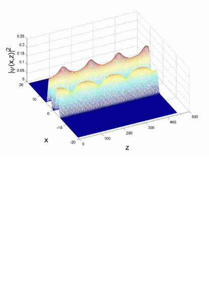
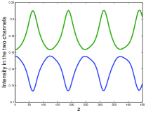
Figure 8: (Color online) Transformation of an unstable narrow symmetric stationary soliton into a persistent breather, initiated by a weak initial perturbation: (a) the evolution of the local intentisty; (b) peak intensities in the two channels versus $z$. Parameters of the two-channel trapping potential are $V_{0}=3$, $D=4$, $L=2$, and the propagation constant of the unperturbed state is $k=$ $2.85$. The calculation based on Eq. (12) yields instability growth rate $\sigma\approx 0.05$ for the underlying stationary soliton.

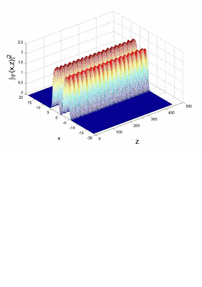
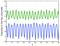
Figure 9: (Color online) The same as in Fig. 8 (with the same values of the parameters) for an unstable broad antisymmetric soliton. In this case, the instability growth rate for the underlying stationary soliton is $\sigma\approx 0.25$.

The breathers formed from the unstable symmetric and antisymmetric solitons, such as those displayed in Figs. 8 and 9, feature not only the phase shift of $\pi$ between the oscillations in the two channels, but also SSB (spontaneous symmetry breaking), as clearly manifested, in panels (b) of the figures, by the difference in the peak powers in the channels. Additional simulations demonstrate that, unlike the period of the oscillations, the size of the symmetry breaking, if measured as the difference between the maximum values of the peak powers, practically does not depend on the size of the initial perturbation.

In most cases, the breathers formed from unstable solitons exhibit strictly periodic oscillations, as in Figs. 8(a) and 11. However, one species of the unstable stationary states, viz., broad antisymmetric ones, may transform itself into a breather which features (seemingly) chaotic oscillations. Some irregularity is seen in the evolution of the peak powers in Fig. 9(b). The increase of the coupling between the channels, i.e., a decrease in $L$, makes the oscillations manifestly chaotic, see Fig. 10. Note that the instability growth rate of the unstable solitons, $\sigma$, which give rise to chaotic breathers is much higher than in cases when periodic breathers are generated: for instance, it is, respectively, $\sigma\approx 0.05$ and $\sigma\approx 0.5$ in Figs. 8 and 10. On the other hand, Fig. 10(b) suggests that the chaotic breather restores, on average, the originally broken dynamical symmetry between the two channels. Indeed, in that case the average values of the peak power in the channels are equal, both being $1.955$.

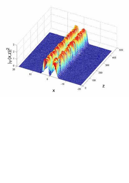
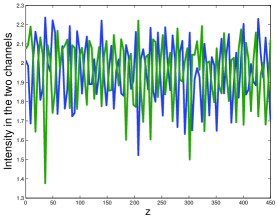
Figure 10: (Color online) The same as in Fig. 9, with a difference that the separation between the two channels is $L=2$ instead of $L=1$. The stronger coupling between the channels results in the formation of a chaotic breather. The instability growth rate for the underlying stationary soliton is $\sigma\approx 0.5$.

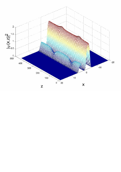
Figure 11: (Color online) The same as in Fig. 8 for an unstable unipolar composite state. Parameters are $V_{0}=3$, $D=4$, $L=2$, and $k=2.85$. The instability growth rate for this state is $\sigma\approx 0.05$.

IV Bifurcation diagrams

The global description of various stationary soliton families found in the present model, and of links between them is provided by diagrams that show the integral power of relevant solutions, $P$, as a function of the propagation constant, $k$, along with diagrams that display an effective asymmetry of the solutions versus $P$. The latter characteristic is defined as follows:

$$\varepsilon\equiv\frac{\int_{0}^{+\infty}\left|\psi(x)\right|^{2}dx-\int_{-\infty}^{0}\left|\psi(x)\right|^{2}dx}{P}$$ (13)

[recall $P\equiv\int_{-\infty}^{0}\left|\psi(x)\right|^{2}dx+\int_{0}^{+\infty}\left|\psi(x)\right|^{2}dx$ is the total power of the spatial soliton]. The form of the bifurcation diagrams turns out to be quite different in the cases of strong and weak coupling between the two channels, which correspond to small and large values of thickness $L$ of the barrier between the channels. These two situations are presented below separately, with labels identifying the eight basic types of the solution branches in the plots as follows:

$\mathrm{A}$ and $\mathrm{B}$ – symmetric stationary solutions of the broad and narrow types, respectively;

$\mathrm{A}^{\prime}$ and $\mathrm{B}^{\prime}$ – antisymmetric solutions of the broad and narrow types, respectively;

$\mathrm{C}$ and $\mathrm{C}^{\prime}$ – unipolar and bipolar composite states, respectively;

$\mathrm{D}$ and $\mathrm{E}$ – single-sided broad and narrow solutions, respectively.

IV.1 Strong coupling

Generic bifurcation diagrams for the system with a relatively strong interaction between the beams trapped in the two channels are displayed in Figs. 12 and 13. Following the usual convention, continuous and dashed curves in these plots represent stable and unstable solution branches. Discontinuities at turning points in panels 12(a) and 13(a) are due to the (well-known) problem with poor convergence of numerical solutions in a vicinity of such points. For the same reason, the left, nearly vertical, segments of branch $\mathrm{E}$ in Figs. 12(b) and 13(b) (and also in Figs. 14(b) and 15(b) below) were found with a low accuracy, therefore they are shown by dots. Note that values of $k$ at the two right turning points in Figs. 12(a) and 13(a), as well as in Figs. 14(a) and 15(a) below, are close but not equal.

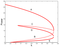
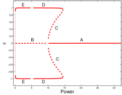
Figure 12: (Color online) Generic examples of the bifurcation diagrams in the strongly-coupled system, for $V_{0}=3$, $D=8$, $L=1$. This set of the diagrams displays symmetric, unipolar composite, and single-sided branches of the spatial-soliton solutions. (a) The integral power ($P$) versus the propagation constant; (b) the asymmetry parameter (defined as per Eq. (13)) versus $P$. Labels A, B, C, D and E are defined in the text.

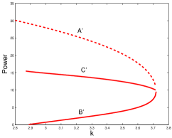
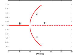
Figure 13: (Color online) The same as in Fig. 12, but for branches of the antisymmetric and bipolar composite states. Labels A^′, B^′, and C^′ are defined in the text.

We stress that the bifurcations at points where branches $\mathrm{A}$, $\mathrm{B}$ and $\mathrm{C}$ meet in Fig. 12(a), as well as where $\mathrm{A}^{\prime}$, $\mathrm{B}^{\prime}$ and $\mathrm{C}^{\prime}$ meet in Fig. 13(a), actually involve not three but four different branches (in compliance with general principles of the bifurcation theory JosephIooss ). Indeed, Figs. 12(b) and 13(b) clearly demonstrate that branches $\mathrm{C}$ and $\mathrm{C}^{\prime}$ exist each in two copies, that are mirror images to each other: one is composed of a narrow soliton in the left channel and a broad one in the right channel, and vice versa. It is noteworthy that branches $\mathrm{C}$ and $\mathrm{D}$, which represent, severally, the unstable unipolar composite solitons and stable single-sided broad solitons, meet and disappear through a tangent (alias saddle-node JosephIooss ) bifurcation in Fig. 10(a). Also worthy to note is the fact that branches $\mathrm{D}$ and $\mathrm{E}$, which meet and disappear at the lower left turning point in Fig. 10(a), are both stable, contrary to the “naive” expectation that one of them ought to be unstable (this fact was already discovered in the single-channel CQ model we ).

The bifurcation diagram in the plane of $P$ and $\varepsilon$ actually describes the SSB, in terms of stationary solutions. Note that the diagram in Fig. 12(b) features a loop, which is a characteristic feature of the SSB in models with saturable Canberra and CQ nonlinearities. In the latter context, closed bifurcation loops were found in the discrete (lattice) version of the CQ model Ricardo , and in a system of two linearly coupled NLS equations with the CQ nonlinearity Lior . The presence of the bifurcation loop implies that the broken symmetry is eventually restored, under the action of the quintic term. On the other hand, the diagram in the same plane for solution branches $\mathrm{A}^{\prime}$, $\mathrm{B}^{\prime}$ and $\mathrm{C}^{\prime}$ in Fig. 13(b) does not display a closed loop. In fact, two mutually symmetric branches $\mathrm{C}^{\prime}$ in this diagram terminate because of difficulties with the numerical continuation to larger values of $P$; on the other hand, the branch of broad antisymmetric solitons, $\mathrm{A}^{\prime}$, can be continued easily, and the continuation does not reveal its stabilization at any particular value of $P$ (in direct simulations, the broad antisymmetric soliton always turns into a persistent breather, cf. Fig. 8(b)), hence it is plausible that the configuration observed in Fig. 11(b) is not going to form a closed bifurcation loop. As concerns the continuation of branch $\mathrm{A}$ in Fig. 12(b) (and also in Fig. 14(b) below) to $P\rightarrow\infty$, this happens with $k\rightarrow k_{\max}\equiv 3/4$, when state $\mathrm{A}$ becomes asymptotically similar to CW state $\psi_{\mathrm{CW}}^{(+)}$, see Eq. (5). Similarly, state $\mathrm{A}^{\prime}$ in Figs. 13(b), and also in 15(b) below, become similar, in the same limit to a dark soliton in the free space.

IV.2 Weak coupling

At essentially larger values of the thickness of the buffer layer between the channels ($L$), which implies weak interaction between them, the character of the bifurcation diagrams changes qualitatively, as shown in Figs. 14 and 15. In this situation, the tangent bifurcation through which branches $\mathrm{C}$ and $\mathrm{D}$ disappeared in the case of the strong inter-channel coupling does not take place, cf. Fig. 12(a). Instead, there occurs another bifurcation that involves solution families $\mathrm{C}$, $\mathrm{C}^{\prime}$ and $\mathrm{D}$ (in fact, family $\mathrm{D}$ of the stable broad single-sided solutions consists of two branches, one to the right of the bifurcation point, and the continuation to the left of it). This bifurcation manifests itself in the diagrams that involve the sets of both symmetric and antisymmetric states, i.e., $\left(\mathrm{A},\mathrm{B},\mathrm{C}\right)$ in Fig. 14(a), and $\left(\mathrm{A}^{\prime},\mathrm{B}^{\prime},\mathrm{C}^{\prime}\right)$ in Fig. 15(a).

In the plane of $\left(P,\varepsilon\right)$, the continuation of branches $\mathrm{D}$ toward larger values of the power does not reveal any trend to forming a closed loop. Instead, the branches remain virtually identical to lines $\varepsilon=\pm 1$, which is obvious in Figs. 14(b) and 15(b). This feature is explained by the propensity of the broad single-sided soliton to turn into the front state (which obviously has $\varepsilon=\pm 1$), as shown above in Fig. 5.

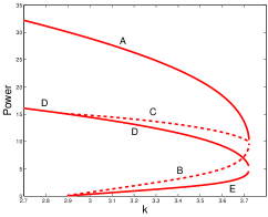
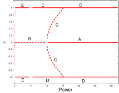
Figure 14: (Color online) The same as in Fig. 12, but for the weakly-coupled system, with $V_{0}=3$, $D=8$, and $L=8$.

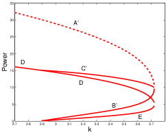
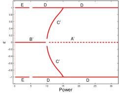
Figure 15: (Color online) The same as in Fig. 13, with parameters identical to those in Fig. 14, but also including branches $\mathrm{D}$ and $\mathrm{E}$ of the single-sided solitons.

In both cases of the strong and weak coupling, the model gives rise to four bifurcations: those involving sets of branches $\left(\mathrm{A},\mathrm{B},\mathrm{C}\right)$, $\left(\mathrm{A}^{\prime},\mathrm{B}^{\prime},\mathrm{C}^{\prime}\right)$, $\left(\mathrm{C},\mathrm{D}\right)$ and $\left(\mathrm{D},\mathrm{E}\right)$ in Figs. 12 and 13, and sets $\left(\mathrm{A},\mathrm{B},\mathrm{C}\right)$, $\left(\mathrm{A}^{\prime},\mathrm{B}^{\prime},\mathrm{C}^{\prime}\right)$, $\left(\mathrm{C},\mathrm{C}^{\prime},\mathrm{D}\right)$ and $\left(\mathrm{D},\mathrm{E}\right)$ in Figs. 14 and 15. The transition between the bifurcation diagrams corresponding to these two cases amounts to the well-known generic type of the rearrangement, when a branch splits off from a pitchfork bifurcation pattern, leaving behind a bifurcation of the tangent type (in the present situation, the detaching branch is $\mathrm{C}^{\prime}$, as suggested by Fig. 11(a)). We did not aim to find an exact value of $L$ (for fixed $V_{0}$ and $D$) at which the bifurcation changes its character.

V Conclusion

The aim of this work was to explore spatial solitons that can be trapped in a planar waveguide which combines two fundamental ingredients, namely, the dual-channel configuration and competing (cubic-quintic) nonlinearity. We have found eight species of the solitons, including symmetric and antisymmetric ones of the broad and narrow types, unipolar and bipolar composite solitons, and the broad and narrow species of single-sided solitons. In contrast to this situation, previously studied models combining two-channel traps with non-competing nonlinearities (of the cubic and saturable types) gave rise to three species of the states (symmetric, antisymmetric, and single-sided asymmetric ones). The stability of the eight families was explored through the computation of perturbation eigenvalues and by means of direct simulations. It has been concluded that three families are unstable, viz., narrow symmetric, broad antisymmetric, and unipolar composite states, each of the other five species being stable as a whole. All instabilities against infinitesimal perturbations are accounted for by real eigenvalues. However, unstable solitons are not destroyed by the instability, but rather turn into robust breathers, which feature dynamical SSB (spontaneousness symmetry breaking), between the field intensities in the two channels. The breathers generated by strongly unstable broad antisymmetric solitons turn out to be chaotic (rather than periodic). It is interesting that the broad and narrow spatial solitons of the antisymmetric type switch their stability in the limit when the two-channel setting is going to merge into the single-channel one: the broad state becomes stable, while the narrow one is destabilized. Four bifurcations linking different branches of the stationary states have been found. The bifurcation diagrams may be of two different types, corresponding to the strong or weak coupling between the two channels. In the latter case, the bifurcation diagram involving the symmetric and unipolar composite states features a closed loop (as seen in Fig. 12). An additional finding, which is relevant to the single-channel setting as well, is the stable front-shaped state (as shown in Fig. 5).

Numerous stable spatial solitons possible in this model may find applications to all-optical data-processing schemes. Moreover, the potential of the two-channel model is not exhausted by the analysis of the eight types of the trapped states reported in this work. Additional species of spatial soliton are possible in it, the form of symmetric, antisymmetric, composite and single-sided configurations based on stable broad dipoles (intrinsically antisymmetric states) trapped in each channel, as well as complexes involving a fundamental soliton in one channel and a broad dipole in the other. A challenging generalization is also possible for a two-dimensional model with the CQ nonlinearity and two parallel trapping channels. In that case, each channel may carry a fundamental two-dimensional soliton or a vortex.

References

- (1) S. Maneuf, F. Reynaud, Opt. Commun. 65 (1988) 325; J. S. Aitchison, A. M. Weiner, Y. Silberberg, M. K. Oliver, J. L. Jackel, D. E. Leaird, E. M. Vogel, P. W. E. Smith, Opt. Lett. 15 (1990) 471.
- (2) B. A. Malomed, Z. H. Wang, P. L. Chu, G. D. Peng (1999) J. Opt. Soc. Am. B 16, 1197.
- (3) J. W. Fleischer, M. Segev, N. K. Efremidis, D. N. Christodoulides (2003) Nature 422, 147.
- (4) G. L. Alfimov, V. V. Konotop, M. Salerno, Europhys. Lett. 58 (2002) 7.
- (5) L. Fallani, C. Fort, M. Inguscio, Riv. Nuovo Cim. 28 (2005) 1; O. Morsch M. Oberthaler, Rev. Mod. Phys. 78 (2006) 179.
- (6) W. D. Li, A. Smerzi, Phys. Rev. E 70 (2004) 016605.
- (7) B. T. Seaman, L. D. Carr, M. J. Holl, Phys. Rev. A 71 (2005) 033622; ibid. A 72 (2005) 033602; I. Danshita, S. Tsuchiya, ibid. A 75 (2007) 033612.
- (8) F. Smektala, C. Quemard, V. Couderc, A. Barthélémy, J. Non-Cryst. Solids 274 (2000) 232; K. Ogusu, J. Yamasaki, S. Maeda, M. Kitao, M. Minakata, Opt. Lett. 29 (2004) 265.
- (9) C. Zhan, D. Zhang, D. Zhu, D. Wang, Y. Li, D. Li, Z. Lu, L. Zhao, Y. Nie, J. Opt. Soc. Am. B 19 (2002) 369.
- (10) G. Boudebs, S. Cherukulappurath, H. Leblond, J. Troles, F. Smektala, F. Sanchez, Opt. Commun. 219 (2003) 427; F. Sanchez, G. Boudebs, S. Cherukulappurath, H. Leblond, J. Troles, F. Smektala, J. Nonlin. Opt. Phys. & Mat. 13(2004) 7.
- (11) Y.-F. Chen, K. Beckwitt, F. W. Wise, B. A. Malomed, Phys. Rev. E 70 (2004) 046610.
- (12) G. S. Agarwal and S. Dutta Gupta, Phys. Rev. A 38 (1988) 5678.
- (13) E. L. Falcão-Filho, C.B. de Araújo, and J. J. Rodrigues, Jr., J. Opt. Soc. Am. B 24 (2007) 2948.
- (14) B. V. Gisin, R. Driben, B. A. Malomed, J. Opt. B: Quant. Semiclass. Opt. 6 (2004) S259.
- (15) I. M. Merhasin, B. V. Gisin, R. Driben, B. A. Malomed, Phys. Rev. E 71 (2005) 016613.
- (16) Kh. I. Pushkarov, D. I. Pushkarov, I. V. Tomov, Opt. Quant. Electr. 11 (1979) 471; S. Cowan, R. H. Enns, S. S. Rangnekar, S. S. Sanghera, Can. J. Phys. 64 (1986) 311.
- (17) G. Iooss D. D. Joseph, Elementary Stability Bifurcation Theory (Springer-Verlag: New York, 1980).
- (18) B. V. Gisin, A. A. Hardy, Phys. Rev. A 48 (1993) 3466.
- (19) J. Wang, F. Ye, L. Dong, T. Cai, Y.-P. Li, Phys. Lett. A 339 (2005) 74.
- (20) M. Albiez, R. Gati, J. Fölling, S. Hunsmann, M. Cristiani, M. K. Oberthaler, Phys. Rev. Lett. 95 (2005) 010402; R. Gati, M. Albiez, J. Fölling, B. Hemmerling, M. K. Oberthaler, Appl. Phys. B 82 (2006) 207.
- (21) A. Smerzi, S. Fantoni, S. Giovanazzi, S. R. Shenoy, Phys. Rev. Lett. 79 (1997) 4950; S. Raghavan, A. Smerzi, S. Fantoni, S. R. Shenoy, Phys. Rev. A 59 (1999) 620; R. K. Jackson M. Weinstein, J. Stat. Phys. 116 (2004) 881; K. W. Mahmud, H. Perry, W. P. Reinhardt, Phys. Rev. A 71 (2005) 023615; T. Kapitula, P. G. Kevrekidis, Nonlinearity 18 (2005) 2491; E. Infeld, P. Ziń, J. Gocalek M. Trippenbach, Phys. Rev. E 74 (2006) 026610; G. Theocharis, P. G. Kevrekidis, D. J. Frantzeskakis P. Schmelcher, ibid. E 74 (2006) 056608.
- (22) A. W. Snyder, D. J. Mitchell, L. Poladian, D. R. Rowl, Y. Chen, J. Opt. Soc. Am. B 8 (1991) 2102.
- (23) P. G. Kevrekidis, Z. Chen, B. A. Malomed, D. J. Frantzeskakis, M. I. Weinstein, Phys. Lett. A 340 (2005) 275.
- (24) M. Matuszewski, B. A. Malomed, M. Trippenbach, Phys. Rev. A 75 (2007) 063621.
- (25) R. Driben, B. A. Malomed, P. L. Chu, J. Phys. B: At. Mol. Opt. Phys. 39 (2006) 2455.
- (26) P. G. Kevrekidis, B. A. Malomed, D. J. Frantzeskakis, A. R. Bishop, H. E. Nistazakis, R. Carretero-González, Math. Comp. Sim. 69 (2005) 334.
- (27) P. G. Kevrekidis, D. J. Frantzeskakis, B. A. Malomed, A. R. Bishop, I. G. Kevrekidis, New J. Phys. 5 (2003) 64.1-64.17.
- (28) D. Mihalache, D. M. Baboiu, M. Ciumac, D. Mazilu, Opt. Quant. Electr. 26 (1994) S311; B. V. Gisin A. A. Hardy, ibid. 27 (1995) 565; B. V. Gisin, A. A. Hardy, B. A. Malomed, Phys. Rev. E 50 (1994) 3274; B. V. Gisin, A. Kaplan, B. A. Malomed, ibid. 62 (2000) 2804.
- (29) T. Kapitula, P. G. Kevrekidis, B. A. Malomed, Phys. Rev. E 63 (2001)036604; P. G. Kevrekidis, B. A. Malomed, A. R. Bishop, J. Phys. A Math. Gen. 34 (2001) 9615.
- (30) D. L. Feder, M. S. Pindzola, L. A. Collins, B. I. Schneider, C. W. Clark, Phys. Rev. A 62 (2000) 053606; L. D. Carr, J. Br, S. Burger, A. Sanpera, ibid. 63 (2001) 051601(R); P. G. Kevrekidis, R. Carretero-González, G. Theocharis, D. J. Frantzeskakis, B. A. Malomed, ibid. 68 (2003) 035602; G. Theocharis, P. G. Kevrekidis, M. K. Oberthaler, D. J. Frantzeskakis, ibid 76 (2007) 045601.
- (31) R. Carretero-González, J. D. Talley, C. Chong, B. A. Malomed, Physica D 216 (2006) 77.
- (32) L. Albuch B. A. Malomed, Math. Comp. Sim. 74 (2007) 312.