Polyakov loops and SU(2) staggered Dirac spectra

Abstract:

We consider the spectrum of the staggered Dirac operator with SU(2) gauge fields. Our study is motivated by the fact that the antiunitary symmetries of this operator are different from those of the SU(2) continuum Dirac operator. In this contribution, we investigate in some detail staggered eigenvalue spectra close to the free limit. Numerical experiments in the quenched approximation and at very large $\beta$-values show that the eigenvalues occur in clusters consisting of eight eigenvalues each. We can predict the locations of these clusters for a given configuration very accurately by an analytical formula involving Polyakov loops and boundary conditions. The spacing distribution of the eigenvalues within the clusters agrees with the chiral symplectic ensemble of random matrix theory, in agreement with theoretical expectations, whereas the spacing distribution between the clusters tends towards Poisson behavior.

1 Introduction

Random matrix theory (RMT) [1] accurately describes eigenvalue correlations in complex systems. More precisely, if we consider a quantum system governed by a Hamiltonian $H$ whose classical counterpart is chaotic, then the statistical properties of the eigenvalue spectrum of $H$ can be modeled by an ensemble of matrices with random entries (distributed according to some statistical weight) and with the same global symmetries as $H$. This description is insensitive to the details of the interaction and predicts universal features that are unveiled when different spectra are rescaled (unfolded) to the same mean density.

Among the many applications of RMT in mathematics and in physics, a particularly interesting one is relevant for the description of the spectrum of the Dirac operator in quantum chromodynamics. QCD in the $\varepsilon$-regime can be described by a chiral RMT with the same chiral and flavor symmetries as QCD [2]. This approach can also be extended to non-vanishing temperature and/or chemical potential and has been confirmed in many numerical studies. In this formulation, the anti-Hermitian massless Dirac operator $D=\gamma_{\mu}\left(\partial_{\mu}+iA_{\mu}\right)$ is described in terms of a matrix with an off-diagonal block structure,

$$D\to\left(\begin{tabular}[]{cc}0&$iW$\\ $iW^{\dagger}$&0\\ \end{tabular}\right)\>,$$ (1)

where $W$ is a complex $(n+\nu)\times n$ matrix and $\nu$ plays the role of the topological charge.

Depending on the color gauge group $G$ and on the fermion field representation, the Dirac operator may also be invariant under some discrete antiunitary symmetries, leading to the following symmetry classes [3]:

1. For $G=\text{SU}(2)$ and fermions in the fundamental representation, the pseudo-real nature of the group generators allows us to recast the Dirac operator in a form with real matrix entries. The corresponding matrix ensemble is the chiral orthogonal ensemble (chOE) with Dyson index $\beta_{D}=1$.

2. For $G=\text{SU}(N_{C})$ with $N_{C}\geq 3$ and fermions in the fundamental representation, the Dirac operator generically has complex entries. The appropriate matrix ensemble is the chiral unitary ensemble (chUE) with Dyson index $\beta_{D}=2$.

3. For gauge group $G=\text{SU}(N_{C})$ and fermions in the adjoint representation, the generators are antisymmetric matrices with imaginary entries, and the Dirac operator can be written as a matrix of real quaternions. The associated matrix ensemble is the chiral symplectic ensemble (chSE) with Dyson index $\beta_{D}=4$.

The behavior of the universal quantities depends on the symmetry classes listed above. In particular, the probability density $P(s)$ for the spacing $s$ of adjacent unfolded levels can be computed exactly and is well approximated by the Wigner surmise,

$$P(s)=a\,s^{\beta_{D}}e^{-bs^{2}}\quad\text{with}\quad a=2\,\frac{\Gamma^{\beta_{D}+1}\left(\beta_{D}/2+1\right)}{\Gamma^{\beta_{D}+2}\left((\beta_{D}+1)/2\right)}\>,\quad b=\frac{\Gamma^{2}\left(\beta_{D}/2+1\right)}{\Gamma^{2}\left((\beta_{D}+1)/2\right)}\>.$$ (2)

For quantum systems whose classical analog is integrable, $P(s)$ is given by the result for a Poisson process, $P(s)=e^{-s}$.

The massless staggered Dirac operator on a lattice in $d$ dimensions with lattice spacing $a$,

$$(D_{\text{KS}})_{x,y}=\frac{1}{2a}\sum_{\mu=1}^{d}(-1)^{\sum\limits_{\nu<\mu}\!\!x_{\nu}}\left[\delta_{x+\hat{\mu},y}U_{\mu}^{\dagger}(x)-\delta_{x-\hat{\mu},y}U_{\mu}(x-\hat{\mu})\right]\>,$$ (3)

which is widely used in numerical simulations, exhibits a peculiar feature: For gauge group SU(2) and fundamental fermions, its antiunitary symmetry is that of the chSE [4] instead of the chOE symmetry of the continuum operator. This discrepancy is due to the replacement of the $\gamma$-matrices by the staggered phases in $D_{\text{KS}}$. Fig. 1 confirms the expectation using $P(s)$ as an example.

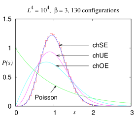
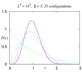
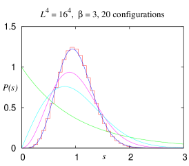
Figure 1: The distribution of the unfolded level spacing $s$ obtained for different lattice sizes from the SU(2) staggered Dirac operator with fundamental fermions and gauge action parameter $\beta=4/g^{2}=3.0$ (histograms) is consistent with the chSE, which is not the symmetry of the continuum Dirac operator.

A transition of the symmetry properties of the staggered Dirac operator from chSE to chOE is expected in the continuum limit. A first indication of such a transition has been reported in Ref. [5]. We plan to study this transition in more detail, but here we first consider a numerically cheaper case, namely the free limit. This limit is approached by increasing $\beta$ at fixed (or mildly varying) lattice size, i.e., the physical volume is shrinking to zero. From the RMT point of view, this limit is interesting since it might result in a transition to Poisson behavior in, e.g., $P(s)$. We shall see that the situation is actually a bit more complicated.

2 The Dirac spectrum of vacuum configurations and the influence of Polyakov loops

In this section we present a short theoretical interlude in preparation for our numerical results. Let us consider a particular gauge configuration. For reasons that will become clear below, we now construct a corresponding vacuum configuration (i.e., a configuration with all plaquettes equal to unity) that is built from uniform links in an Abelian subgroup of SU(2) which reproduce the average traced Polyakov loops $P_{\mu}$ (for all directions $\mu$) of the configuration under consideration. The eigenvalue spectrum of the staggered Dirac operator (3) can be computed analytically for such a vacuum configuration. If the lattice extent in the $\mu$-direction is $L_{\mu}$, we obtain

$$\lambda=\pm i\sqrt{\sum_{\mu=1}^{d}\sin^{2}\left[\frac{2\pi}{L_{\mu}}\left(k_{\mu}+c_{\mu}+\frac{\arccos P_{\mu}}{2\pi}\right)\right]}\quad\text{with }\>k_{\mu}\in\mathbb{N}\>,\;0\leq k_{\mu}<\frac{L_{\mu}}{2}\>,$$ (4)

where $c_{\mu}=0$ $\left(c_{\mu}=\frac{1}{2}\right)$ for (anti-) periodic boundary conditions (b.c.s) of the Dirac operator in direction $\mu$. In the free limit, i.e., for $\beta\to\infty$, the Polyakov loops take values in the center $\mathbb{Z}_{2}$ of SU(2), i.e., $P_{\mu}=\pm 1$. In this case it is clear from Eq. (4) that changing $P_{\mu}$ from $+1$ to $-1$, or vice versa, is equivalent to switching between periodic and antiperiodic b.c.s in that direction. In the following we always use (anti-) periodic b.c.s for $\mu=1$, 2, 3 ($\mu=4$). Close to the free limit, i.e., for large values of $\beta$, the distribution of $P_{\mu}$ is peaked at $\pm 1$. The eigenvalues predicted by Eq. (4) are degenerate, see below.

3 Numerical results for the eigenvalue spectrum close to the free limit

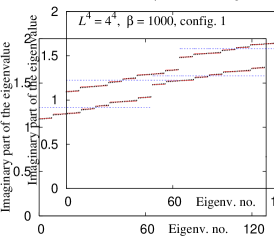
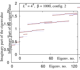
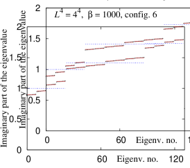
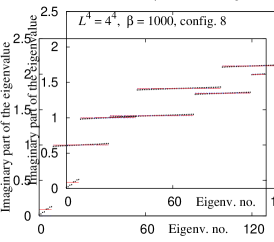
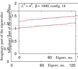
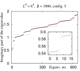
Figure 2: Separation of scales in the level spacings close to the free limit. The eigenvalues obtained for each configuration (black dots) arrange themselves in clusters of eight. These clusters are spread about the well-separated plateaux corresponding to the free case (dashed blue lines). Eq. (4) yields an accurate prediction for the location of each cluster (solid red lines). The different plateau structures are due to the different signs of $P_{\mu}\approx\pm 1$ in each configuration. The last plot confirms that the agreement between the data and Eq. (4) persists on larger lattices, for which the theoretical formula predicts more clusters.

When $\beta$ is increased to very large values, we observe that the eigenvalue spectrum of $D_{\text{KS}}$ arranges itself as shown in Fig. 2. Only the eigenvalues with positive imaginary part are plotted, and an overall double (Kramers) degeneracy [6] has been divided out from all of our results. The dashed blue lines, which will be called plateaux in the following, correspond to the highly degenerate eigenvalues predicted by Eq. (4) in the free limit, i.e., for $P_{\mu}=\pm 1$. The numerically obtained eigenvalues form clusters consisting of eight eigenvalues each, and these clusters are located close to the plateaux of the free limit. We observe a clear separation of three energy scales (from largest to smallest),

1. the spacings between the plateaux of the free limit,

2. the spacings between adjacent clusters (which, by definition, do not overlap), and

3. the spacings between adjacent eigenvalues within a cluster.

The question now arises to what extent the locations of the clusters for a particular configuration can be described by the levels obtained from Eq. (4) for the vacuum configuration constructed as described in Sec. 2. The answer is given by the solid red lines, which correspond to the predictions of Eq. (4) using the $P_{\mu}$ computed from the configuration under consideration. These lines are essentially hidden by the data points and thus give very good approximations to the cluster locations. This statement holds for all configurations, some of which are shown in Fig. 2.

We can understand the observation that the clusters contain eight nearly degenerate eigenvalues. A careful analysis shows that the eigenvalues predicted by Eq. (4) have a multiplicity of $2^{d}$. For $d=4$, this predicts an eightfold degeneracy in addition to Kramers’ degeneracy. A small perturbation of the vacuum configuration lifts this eightfold degeneracy but not the Kramers degeneracy, which is exact for $D_{\text{KS}}$.

We also remark that in the continuum limit, in which the lattice spacing goes to zero at fixed physical volume, the eigenvalues of $D_{\text{KS}}$ should arrange themselves in multiplets corresponding to the taste degeneracy of staggered fermions. This effect was observed for SU(3) [7] (quadruplets) and SU(2) [5] (doublets) for improved versions of $D_{\text{KS}}$, but it should not be confused with the effect we are studying here.

Our observations may be related to other recent work [8] discussing the connection between the spectrum of the Dirac operator (which is relevant for chiral symmetry breaking) and the Polyakov loop (which is an order parameter for confinement in the quenched theory).

4 Spectral fluctuations on different scales

We now turn to a study of spectral correlations close to the free limit, using again the nearest-neighbor spacing distribution $P(s)$ as an example. To construct $P(s)$, the average spectral density must be separated from the spectral fluctuations by an unfolding procedure. Because of the separation of scales observed above, a uniform unfolding of the entire spectral density is not sensible close to the free limit. Rather, we should consider the spectral fluctuations separately on the three scales we identified.

First, we construct $P(s)$ for the level spacings within the clusters by unfolding the spectral density only within a given cluster and then averaging $P(s)$ over all clusters. Fig. 3 (left) shows that $P(s)$ within the clusters continues to agree with the chSE even for very large values of $\beta$. This is consistent with the theoretical expectation, since the perturbation that lifts the degeneracy of the eigenvalues in each cluster has the same symmetries as the full $D_{\text{KS}}$ operator, which are those of the chSE.

Second, to construct $P(s)$ for the spacings between clusters, we define a cluster by the average of its eight members and unfold the density of the clusters. Fig. 3 (right) shows that the resulting $P(s)$ differs from the chSE. It also differs from the Poisson distribution, but we believe that this is due to the small lattice size and to the fact that on a $10^{4}$ lattice the free staggered operator has many “accidental” degeneracies. These degeneracies can be removed by choosing a lattice with $L_{\mu}=2\ell_{\mu}$, where the $\ell_{\mu}$ are four different prime numbers. As an example, we generated quenched configurations close to the free limit ($\beta=10000$) for a $34\times 38\times 46\times 58$ lattice, computed the averaged traced Polyakov loops $P_{\mu}$ and used these to calculate the “cluster spectrum” according to Eq. (4). The resulting $P(s)$ is shown in Fig. 4 (left) and now agrees with the Poisson distribution.

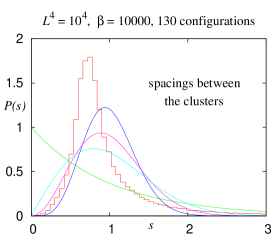
Figure 3: $P(s)$ for the eigenvalue spacings within the clusters (left) and for the spacings between clusters (right), both for $L^{4}=10^{4}$ and $\beta=10000$.

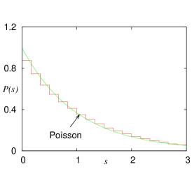
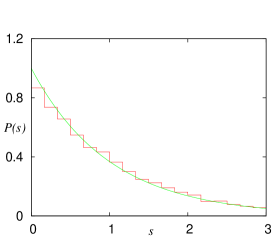
Figure 4: $P(s)$ for the “cluster spectrum” predicted by Eq. (4) for a single configuration on a $34\times 38\times 46\times 58$ lattice at $\beta=10000$ (left) and $P(s)$ for the free Dirac eigenvalues (or plateaux) on the same lattice (right). Both agree with the Poisson distribution.

Third, we consider $P(s)$ for the spacings between the free eigenvalues (or plateaux), which are known analytically (Eq. (4) with $P_{\mu}=\pm 1$). Again it is sensible to remove accidental degeneracies by choosing a “prime lattice”. The result for a $34\times 38\times 46\times 58$ lattice, obtained after unfolding the free eigenvalues, is shown in Fig. 4 (right) and agrees with Poisson as expected [9].

Although the two plots in Fig. 4 look very similar, it should be noted that they come from data at very different scales. The average spacing between the levels of the free spectrum is more than ten times larger than the average spacing between the levels predicted by Eq. (4).

5 Summary and outlook

We have investigated the spectrum of the staggered Dirac operator with SU(2) gauge fields close to the free limit. Three different energy scales emerge:

1. Overall plateau structure: The spectrum arranges itself in clusters of eight eigenvalues each, lying close to the plateaux predicted for the free Dirac operator. The plateau structure only depends on the lattice geometry (i.e., on the $L_{\mu}$ and on the b.c.s) and on the signs of the average traced Polyakov loops in the different directions. (Note that the distribution of the traced Polyakov loops is peaked at $\pm 1$, corresponding to the center elements of SU(2).)

2. Plateau-breaking and cluster separation at an intermediate scale: At a finer scale, the spread of the clusters about the plateaux of the free limit is due to the deviations of the $P_{\mu}$ from $\pm 1$ and can be accurately modeled by Eq. (4).

3. Eigenvalue splitting within the clusters: The system dynamics removes the degeneracy of the eight eigenvalues belonging to the same cluster.

In the regime we have studied, these three scales are well separated and can be unambiguously disentangled from each other.

The nearest-neighbor spacing distribution $P(s)$ computed within the clusters shows a behavior compatible with the chSE, consistent with the symmetries of the staggered Dirac operator. For large enough “prime lattices”, the spacing distributions between the clusters and between the plateaux tends to the Poisson distribution. In the near future, we will also present a study of the spectrum of the Dirac operator for adjoint fermions close to the free limit. Ultimately, of course, we would like to obtain a more detailed understanding of the continuum limit, in which a chSE to chOE (for SU(2) with fundamental fermions) or chOE to chSE (for adjoint fermions) transition is expected.