The Use of Domination Number of a Random Proximity Catch Digraph for Testing Spatial Patterns of Segregation and Association^⋆

Abstract

Priebe et al. (2001) introduced the class cover catch digraphs and computed the distribution of the domination number of such digraphs for one dimensional data. In higher dimensions these calculations are extremely difficult due to the geometry of the proximity regions; and only upper-bounds are available. In this article, we introduce a new type of data-random proximity map and the associated (di)graph in $\mathbb{R}^{d}$. We find the asymptotic distribution of the domination number and use it for testing spatial point patterns of segregation and association.

Keywords: Random digraph; Domination number; Proximity Map; Spatial Point Pattern; Segregation; Association; Delaunay Triangulation

^⋆This research was supported by the Defense Advanced Research Projects Agency as administered by the Air Force Office of Scientific Research under contract DOD F49620-99-1-0213 and by Office of Naval Research Grant N00014-95-1-0777.
Corresponding author.
E-mail address: cep@jhu.edu (C.E. Priebe)

1 Introduction

In a digraph $D=(\mathcal{V},\mathcal{A})$ with vertex set $\mathcal{V}$ and arc (directed edge) set $\mathcal{A}$, a vertex $v$ dominates itself and all vertices of the form $\{u:\,vu\in\mathcal{A}\}$. A dominating set, $S_{D}$, for the digraph $D$ is a subset of $\mathcal{V}$ such that each vertex $v\in\mathcal{V}$ is dominated by a vertex in $S_{D}$. A minimum dominating set, $S_{D}^{*}$, is a dominating set of minimum cardinality; and the domination number, $\gamma(D)$, is defined as $\gamma(D):=|S_{D}^{*}|$, where $|\cdot|$ is the cardinality functional ([West, 2001]). If a minimum dominating set is of size one, we call it a dominating point.

Let $(\Omega,\mathcal{M})$ be a measurable space and consider a function $N:\Omega\times 2^{\Omega}\rightarrow 2^{\Omega}$, where $2^{\Omega}$ represents the power set of $\Omega$. Then given $\mathcal{Y}\subseteq\Omega$, the proximity map $N_{\mathcal{Y}}(\cdot)=N(\cdot,\mathcal{Y}):\Omega\rightarrow 2^{\Omega}$ associates with each point $x\in\Omega$ a proximity region $N_{\mathcal{Y}}(x)\subset\Omega$. The region $N_{\mathcal{Y}}(x)$ depends on the distance between $x$ and $\mathcal{Y}$. For $B\subseteq\Omega$, the $\Gamma_{1}$-region, $\Gamma_{1}(\cdot)=\Gamma_{1}(\cdot,N_{\mathcal{Y}}):\Omega\rightarrow 2^{\Omega}$ associates the region $\Gamma_{1}(B):=\{z\in\Omega:B\subseteq N_{\mathcal{Y}}(z)\}$ with each set $B\subseteq\Omega$. For $x\in\Omega$, we denote $\Gamma_{1}(\{x\})$ as $\Gamma_{1}(x)$.

If $\mathcal{X}_{n}=\{X_{1},X_{2},\cdots,X_{n}\}$ is a set of $\Omega$-valued random variables, then the $N_{\mathcal{Y}}(X_{i})$ (and $\Gamma_{1}(X_{i})$), $i=1,\cdots,n$ are random sets. If the $X_{i}$ are independent and identically distributed, then so are the random sets $N_{\mathcal{Y}}(X_{i})$ (and $\Gamma_{1}(X_{i})$). Furthermore, $\Gamma_{1}(\mathcal{X}_{n})$ is a random set. Notice that $\Gamma_{1}(\mathcal{X}_{n})=\cap_{j=1}^{n}\Gamma_{1}(X_{j})$, since $x\in\Gamma_{1}(\mathcal{X}_{n})$ iff $\mathcal{X}_{n}\subseteq N_{\mathcal{Y}}(x)$ iff $X_{j}\in N_{\mathcal{Y}}(x)$ for all $j=1,\ldots,n$ iff $x\in\Gamma_{1}(X_{j})$ for all $j=1,\ldots,n$ iff $x\in\cap_{j=1}^{n}\Gamma_{1}(X_{j})$.

Consider the data-random proximity catch digraph $D$ with vertex set $\mathcal{V}=\mathcal{X}_{n}$ and arc set $\mathcal{A}$ defined by $(X_{i},X_{j})\in\mathcal{A}\iff X_{j}\in N_{\mathcal{Y}}(X_{i})$. The random digraph $D$ depends on the (joint) distribution of the $X_{i}$ and on the map $N_{\mathcal{Y}}$ (see Priebe et al. (2001) and Priebe et al. (2003)). The adjective proximity — for the catch digraph $D$ and for the map $N_{\mathcal{Y}}$ — comes from thinking of the region $N_{\mathcal{Y}}(x)$ as representing those points in $\Omega$ “close” to $x$ (see, e.g., Toussaint (1980) and Jaromczyk and Toussaint (1992)).

For $X_{1},\cdots,X_{n}\stackrel{{\scriptstyle iid}}{{\sim}}F$ the domination number of the associated data-random proximity catch digraph $D$, denoted $\gamma(\mathcal{X}_{n};F,N_{\mathcal{Y}})$, is the minimum number of points that dominate all points in $\mathcal{X}_{n}$. Note that, $\gamma(\mathcal{X}_{n};F,N_{\mathcal{Y}})=1$ iff $\mathcal{X}_{n}\cap\Gamma_{1}(\mathcal{X}_{n})\not=\emptyset$.

The random variable $\gamma_{n}:=\gamma(\mathcal{X}_{n};F,N_{\mathcal{Y}})$ depends on $\mathcal{X}_{n}$ explicitly, and on $F$ and $N_{\mathcal{Y}}$ implicitly. In general, the expectation $\mathbf{E}\,[\gamma_{n}]$, depends on $n$, $F$, and $N_{\mathcal{Y}}$; $1\leq\mathbf{E}\,[\gamma_{n}]\leq n$; and the variance of $\gamma_{n}$ satisfies, $0\leq\mathbf{Var}\,[\gamma_{n}]\leq n^{2}/4$.

We can also define the regions associated with $\gamma_{n}=k$ for $k\leq n$. For instance, the $\Gamma_{2}$-region for proximity map $N_{\mathcal{Y}}(\cdot)$ and set $B\subset\Omega$ is $\Gamma_{2}(B)=\{(x,y)\in[\Omega\setminus\Gamma_{1}(B)]^{2}:\;B\subseteq N_{\mathcal{Y}}(x)\cup N_{\mathcal{Y}}(y)\}$. In general,

$$\Gamma_{k}(B)=\{(x_{1},x_{2},\ldots,x_{k})\in\Omega^{k}:B\subseteq\cup_{j=1}^{k}N_{\mathcal{Y}}(x_{j})\;\text{ and all possible $m$-permutations $(u_{1},u_{2},\ldots,u_{m})$}\\ \text{ of $(x_{1},x_{2},\ldots,x_{k})$ satisfy }(u_{1},u_{2},\ldots,u_{m})\not\in\Gamma_{m}(B)\text{ for each }m=1,2,\ldots,k-1\}.$$

2 A Class of Proximity Maps and the Corresponding $\Gamma_{1}$-Regions

Let $\Omega=\mathbb{R}^{2}$ and let $\mathcal{Y}=\{\mathsf{y}_{1},\mathsf{y}_{2},\mathsf{y}_{3}\}\subset\mathbb{R}^{2}$ be three non-collinear points. Denote by $T(\mathcal{Y})$ the triangle —including the interior— formed by these three points. The most straightforward extension of the data random proximity catch digraph introduced by Priebe et al. (2001) is the spherical proximity map $N_{S}(x)=B(x,r(x))$ which is the ball centered at $x$ with radius $r(x)=\min_{\mathsf{y}\in\mathcal{Y}}d(x,\mathsf{y})$ or the arc-slice proximity map $N_{AS}(x)=B(x,r(x))\cap T(\mathcal{Y})$. However, both cases suffer from the intractability of the $\Gamma_{1}$-region and hence the intractability of the finite and asymptotic distribution of $\gamma_{n}$. We propose a new class of proximity regions which does not suffer from this drawback.

For $r\in[1,\infty]$ define $N_{\mathcal{Y}}^{r}$ to be the r-factor proximity map and $\Gamma_{1}^{r}$ to be the corresponding $\Gamma_{1}$-region as follows; see also Figures 1 and 2. Let “vertex regions” $R(\mathsf{y}_{1})$, $R(\mathsf{y}_{2})$, $R(\mathsf{y}_{3})$ partition $T(\mathcal{Y})$ using segments from the center of mass of $T(\mathcal{Y})$ to the edge midpoints. For $x\in T(\mathcal{Y})\setminus\mathcal{Y}$, let $v(x)\in\mathcal{Y}$ be the vertex whose region contains $x$; $x\in R(v(x))$. If $x$ falls on the boundary of two vertex regions, we assign $v(x)$ arbitrarily. Let $e(x)$ be the edge of $T(\mathcal{Y})$ opposite $v(x)$. Let $\ell(v(x),x)$ be the line parallel to $e(x)$ through $x$. Let $d(v(x),\ell(v(x),x))$ be the Euclidean (perpendicular) distance from $v(x)$ to $\ell(v(x),x)$. For $r\in[1,\infty)$ let $\ell_{r}(v(x),x)$ be the line parallel to $e(x)$ such that $d(v(x),\ell_{r}(v(x),x))=rd(v(x),\ell(v(x),x))$ and $d(\ell(v(x),x),\ell_{r}(v(x),x))<d(v(x),\ell_{r}(v(x),x))$. Let $T_{r}(x)$ be the triangle similar to and with the same orientation as $T(\mathcal{Y})$ having $v(x)$ as a vertex and $\ell_{r}(v(x),x)$ as the opposite edge. Then the r-factor proximity region $N_{\mathcal{Y}}^{r}(x)$ is defined to be $T_{r}(x)\cap T(\mathcal{Y})$.

To define the $\Gamma_{1}$-region, let $\xi_{j}(x)$ be the line such that $\xi_{j}(x)\cap T(\mathcal{Y})\not=\emptyset$ and $r\,d(\mathsf{y}_{j},\xi_{j}(x))=d(\mathsf{y}_{j},\ell(\mathsf{y}_{j},x))$ for $j=1,2,3$. Then $\Gamma_{1}^{r}(x)=\cup_{j=1}^{3}\bigl{(}\Gamma_{1}^{r}(x)\cap R(\mathsf{y}_{j})\bigr{)}$ where $\Gamma_{1}^{r}(x)\cap R(\mathsf{y}_{j})=\{z\in R(\mathsf{y}_{j}):d(\mathsf{y}_{j},\ell(\mathsf{y}_{j},z))\geq d(\mathsf{y}_{j},\xi_{j}(x)\}$, for $j=1,2,3$. Notice that $r\geq 1$ implies $x\in N_{\mathcal{Y}}^{r}(x)$ and $x\in\Gamma_{1}^{r}(x)$. Furthermore, $\lim_{r\rightarrow\infty}N_{\mathcal{Y}}^{r}(x)=T(\mathcal{Y})$ and $\lim_{r\rightarrow\infty}\Gamma_{1}^{r}(x)=T(\mathcal{Y})$ for all $x\in T(\mathcal{Y})\setminus\mathcal{Y}$, and so we define $N_{\mathcal{Y}}^{\infty}(x)=T(\mathcal{Y})$ and $\Gamma_{1}^{\infty}(x)=T(\mathcal{Y})$ for all such $x$. For $x\in\mathcal{Y}$, we define $N_{\mathcal{Y}}^{r}(x)=\{x\}$ for all $r\in[1,\infty]$.

Notice that $X_{i}\stackrel{{\scriptstyle iid}}{{\sim}}F$, with the additional assumption that the non-degenerate two-dimensional probability density function $f$ exists with $\operatorname{support}(f)\subseteq T(\mathcal{Y})$, implies that the special case in the construction of $N_{\mathcal{Y}}^{r}$ — $X$ falls on the boundary of two vertex regions — occurs with probability zero. Note that for such an $F$, $N_{\mathcal{Y}}^{r}(x)$ is a triangle a.s. and $\Gamma^{r}_{1}(x)$ is a star-shaped polygon (not necessarily convex).

Figure 1: Construction of $r$-factor proximity region, $N_{\mathcal{Y}}^{2}(x)$ (shaded region).

Figure 2: Construction of the $\Gamma_{1}$-region, $\Gamma_{1}^{2}(x)$ (shaded region).

Let $X_{e}:=\operatorname{argmin}_{X\in\mathcal{X}_{n}}d(X,e)$ be the (closest) edge extremum for edge $e$. Then $\Gamma^{r}_{1}(\mathcal{X}_{n})=\cap_{j=1}^{3}\Gamma^{r}_{1}(X_{e_{j}})$, where $e_{j}$ is the edge opposite vertex $\mathsf{y}_{j}$, for $j=1,2,3$. So $\Gamma^{r}_{1}(\mathcal{X}_{n})\cap R(\mathsf{y}_{j})=\{z\in R(\mathsf{y}_{j}):\;d(\mathsf{y}_{j},\ell(\mathsf{y}_{j},z)\geq d(\mathsf{y}_{j},\xi_{j}(X_{e_{j}}))\}$, for $j=1,2,3$.

Let the domination number be $\gamma_{n}(r):=\gamma_{n}(\mathcal{X}_{n};F,N_{\mathcal{Y}}^{r})$ and $X_{[j]}:=\operatorname{argmin}_{X\in\mathcal{X}_{n}\cap R(\mathsf{y}_{j})}d(X,e_{j})$. Then $\gamma_{n}(r)\leq 3$ with probability 1, since $\mathcal{X}_{n}\cap R(\mathsf{y}_{j})\subset N_{\mathcal{Y}}^{r}(X_{[j]})$ for each $j=1,2,3$. Thus

$$1\leq\mathbf{E}\,[\gamma_{n}(r)]\leq 3\text{ and }0\leq\mathbf{Var}\,[\gamma_{n}(r)]\leq 9/4.$$

3 Null Distribution of Domination Number

The null hypothesis for spatial patterns have been a contraversial topic in ecology from the early days. [Gotelli and Graves, 1996] have collected a voluminous literature to present a comprehensive analysis of the use and misuse of null models in ecology community. They also define and attempt to clarify the null model concept as “a pattern-generating model that is based on randomization of ecological data or random sampling from a known or imagined distribution. . . . The randomization is designed to produce a pattern that would be expected in the absence of a particular ecological mechanism.” In other words, the hypothesized null models can be viewed as “thought experiments,” which is conventially used in the physical sciences, and these models provide a statistical baseline for the analysis of the patterns. For statistical testing, the null hypothesis we consider is a type of complete spatial randomness; that is,

$$H_{0}:X_{i}\stackrel{{\scriptstyle iid}}{{\sim}}\mathcal{U}(T(\mathcal{Y}))$$

where $\mathcal{U}(T(\mathcal{Y}))$ is the uniform distribution on $T(\mathcal{Y})$. If it is desired to have the sample size be a random variable, we may consider a spatial Poisson point process on $T(\mathcal{Y})$ as our null hypothesis.

We first present a “geometry invariance” result which allows us to assume $T(\mathcal{Y})$ is the standard equilateral triangle, $T\bigl{(}(0,0),(1,0),\bigl{(}1/2,\sqrt{3}/2\bigr{)}\bigr{)}$, thereby simplifying our subsequent analysis.

Theorem 1: Let $\mathcal{Y}=\{\mathsf{y}_{1},\mathsf{y}_{2},\mathsf{y}_{3}\}\subset\mathbb{R}^{2}$ be three non-collinear points. For $i=1,\cdots,n$, let $X_{i}\stackrel{{\scriptstyle iid}}{{\sim}}F=\mathcal{U}(T(\mathcal{Y}))$, the uniform distribution on the triangle $T(\mathcal{Y})$. Then for any $r\in[1,\infty]$ the distribution of $\gamma(\mathcal{X}_{n};\mathcal{U}(T(\mathcal{Y})),N_{\mathcal{Y}}^{r})$ is independent of $\mathcal{Y}$, and hence the geometry of $T(\mathcal{Y})$.

Proof: A composition of translation, rotation, reflections, and scaling will take any given triangle $T_{o}=T(\{\mathsf{y}_{1},\mathsf{y}_{2},\mathsf{y}_{3}\})$ to the “basic” triangle $T_{b}=T(\{(0,0),(1,0),(c_{1},c_{2})\})$ with $0<c_{1}\leq 1/2$, $c_{2}>0$ and $(1-c_{1})^{2}+c_{2}^{2}\leq 1$, preserving uniformity. The transformation $\phi_{e}:\mathbb{R}^{2}\rightarrow\mathbb{R}^{2}$ given by $\phi_{e}(u,v)=\left(u+\frac{1-2\,c_{1}}{\sqrt{3}}\,v,\frac{\sqrt{3}}{2\,c_{2}}\,v\right)$ takes $T_{b}$ to the equilateral triangle $T_{e}=T(\{(0,0),(1,0),(1/2,\sqrt{3}/2)\})$. Investigation of the Jacobian shows that $\phi_{e}$ also preserves uniformity. Furthermore, the composition of $\phi_{e}$ with the rigid motion transformations maps the boundary of the original triangle, $T_{o}$, to the boundary of the equilateral triangle, $T_{e}$, the median lines of $T_{o}$ to the median lines of $T_{e}$, and lines parallel to the edges of $T_{o}$ to lines parallel to the edges of $T_{e}$. Since the distribution of $\gamma(\mathcal{X}_{n};\mathcal{U}(T(\mathcal{Y})),N_{\mathcal{Y}}^{r})$ involves only probability content of unions and intersections of regions bounded by precisely such lines, and the probability content of such regions is preserved since uniformity is preserved, the desired result follows. $\blacksquare$

Based on Theorem 1 and our uniform null hypothesis, we may assume that $T(\mathcal{Y})$ is a standard equilateral triangle with $\mathcal{Y}=\{(0,0),(1,0),(1/2,\sqrt{3}/2)\}$ henceforth.

For our $r$-factor proximity map and uniform null hypothesis, the asymptotic null distribution of $\gamma_{n}(r):=\gamma(\mathcal{X}_{n};\mathcal{U}(T(\mathcal{Y})),N_{\mathcal{Y}}^{r})$ can be derived as a function of $r$. We denote by $\varsigma^{r}_{\mathcal{Y}}:=\{z\in T(\mathcal{Y}):\;N_{\mathcal{Y}}^{r}(z)=T(\mathcal{Y})\}$ the superset region associated with $N_{\mathcal{Y}}^{r}$ in $T(\mathcal{Y})$. Notice that $\varsigma^{r}_{\mathcal{Y}}\subseteq\Gamma_{1}^{r}(\mathcal{X}_{n})$ for all $r$ and $\mathcal{X}_{n}\cap\varsigma^{r}_{\mathcal{Y}}\not=\emptyset$ implies that $\gamma_{n}(r)=1$.

Proposition 1: The expected area of the the $\Gamma_{1}$-region, $\mathbf{E}\,[A(\Gamma^{r}_{1}(\mathcal{X}_{n}))]$, converges to the area of the superset region, $A(\varsigma^{r}_{\mathcal{Y}})$, as $n\rightarrow\infty$. In particular, $\mathbf{E}\,[A(\Gamma^{3/2}_{1}(\mathcal{X}_{n}))]$, goes to zero at rate $O(n^{-2})$ as $n\rightarrow\infty$.

Proof: See Appendix. $\blacksquare$

As a corollary to the above proposition, we have that $\mathbf{E}\,[A(\Gamma^{r}_{1}(\mathcal{X}_{n}))]\rightarrow A(\varsigma^{r}_{\mathcal{Y}})=0$ for $r\in[1,3/2]$ as $n\rightarrow\infty$. Additionally, $\mathbf{E}\,[A(\Gamma^{r}_{1}(\mathcal{X}_{n}))]\rightarrow A(\varsigma^{r}_{\mathcal{Y}})=(1-3/(2\,r))^{2}\,\sqrt{3}$ for $r\in(3/2,2]$, and $\mathbf{E}\,[A(\Gamma^{r}_{1}(\mathcal{X}_{n}))]\rightarrow A(\varsigma^{r}_{\mathcal{Y}})=\sqrt{3}/4\,(1-3/r^{2})$ for $r\in(2,\infty]$, as $n\rightarrow\infty$.

Theorem 2: The domination number $\gamma_{n}(r)=\gamma(\mathcal{X}_{n};\mathcal{U}(T(\mathcal{Y})),N_{\mathcal{Y}}^{r})$ is degenerate in the limit for $r\in[1,\infty]\setminus\{3/2\}$ as $n\rightarrow\infty$.

Proof: For $r\in[1,3/2)$, $\varsigma^{r}_{\mathcal{Y}}=\emptyset$ and $T(\mathcal{Y})\setminus N_{\mathcal{Y}}^{r}(X_{[j]})$ has positive area for all $j=1,2,3$. Furthermore, $T(\mathcal{Y})\setminus(N_{\mathcal{Y}}^{r}(X_{[j]})\cup N_{\mathcal{Y}}^{r}(X_{[k]}))$ has positive area for all pairs $\{j,k\}\subset\{1,2,3\}$. Recall that $\gamma_{n}(r)\leq 3$ with probability 1 for all $n$ and $r$. Hence $\gamma_{n}(r)\rightarrow 3$ in probability as $n\rightarrow\infty$.

For $r\in(3/2,\infty]$, $\varsigma^{r}_{\mathcal{Y}}$ has positive area, so $\gamma_{n}(r)\rightarrow 1$ in probability as $n\rightarrow\infty$. $\blacksquare$

Theorem 3: For $r=3/2$, $\lim_{n\rightarrow\infty}\gamma_{n}(r)>1$ a.s. In particular

$$\lim_{n\rightarrow\infty}\gamma_{n}(3/2)=\begin{cases}2&\text{wp $\approx$}\quad.7413,\\ 3&\text{wp $\approx$}\quad.2487.\end{cases}$$

Thus $\mathbf{E}\,[\gamma_{n}(3/2)]\rightarrow\mu\approx 2.2587$ as $n\rightarrow\infty$, and $\mathbf{Var}\,[\gamma_{n}(3/2)]\rightarrow\sigma^{2}\approx.1918$ as $n\rightarrow\infty$.

Proof: See Appendix. $\blacksquare$

The finite sample distribution of $\gamma_{n}(3/2)$, and hence the finite sample mean and variance, can be obtained by numerical methods. We estimate the distribution of $\gamma_{n}(3/2)$ for various fixed $n$ empirically. In Table 1, we present empirical estimates for $n=10,20,\ldots,100,200,300$ with $1000$ Monte Carlo replicates. See also Figure 3.

$k\diagdown n$	10	20	30	40	50	60	70	80	90	100	200	300
1	151	82	61	67	50	24	29	21	15	27	10	7
2	602	636	688	670	693	714	739	708	723	718	715	730
3	247	282	251	263	257	262	232	271	262	255	275	263

Table 1: The number of $\gamma_{n}(3/2)=k$ out of $N=1000$ replicates.

Figure 3: Plotted are the empirical estimates of $P(\gamma_{n}(3/2)=k)$ versus various $n$ values.

Theorem 4 Let $\gamma_{n}(r)=\gamma(\mathcal{X}_{n};\mathcal{U}(T(\mathcal{Y})),N_{\mathcal{Y}}^{r})$. Then $r_{1}<r_{2}$ implies $\gamma_{n}(r_{2})<^{ST}\gamma_{n}(r_{1})$.

Proof: Suppose $r_{1}<r_{2}$. Then $P(\gamma_{n}(r_{2})=1)>P(\gamma_{n}(r_{1})=1)$ and $P(\gamma_{n}(r_{2})=2)>P(\gamma_{n}(r_{1})=2)$ and $P(\gamma_{n}(r_{2})=3)<P(\gamma_{n}(r_{1})=3)$. Hence the desired result follows. $\blacksquare$

4 The Null Distribution of the Mean Domination Number in the Multiple Triangle Case

Suppose $\mathcal{Y}$ is a finite collection of points in $\mathbb{R}^{2}$ with $|\mathcal{Y}|\geq 3$. Consider the Delaunay triangulation (assumed to exist) of $\mathcal{Y}$, where $T_{j}$ denotes the $j^{th}$ Delaunay triangle, $J$ denotes the number of triangles, and $C_{H}(\mathcal{Y})$ denotes the convex hull of $\mathcal{Y}$ (Okabe et al. (2000)). We wish to investigate

$$H_{0}:X_{i}\stackrel{{\scriptstyle iid}}{{\sim}}\mathcal{U}(C_{H}(\mathcal{Y}))$$

against segregation and association alternatives (see Section 5).

Figure 4 presents a realization of 1000 observations independent and identically distributed according to $\mathcal{U}(C_{H}(\mathcal{Y}))$ for $|\mathcal{Y}|=10$ and $J=13$.

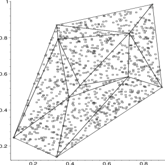
Figure 4: A realization of $H_{0}$ for $|\mathcal{Y}|=10$, $J=13$, and $n=1000$.

The digraph $D$ is constructed using $N_{\mathcal{Y}_{j}}^{r}(\cdot)$ as described above, where for $X_{i}\in T_{j}$ the three points in $\mathcal{Y}$ defining the Delaunay triangle $T_{j}$ are used as $\mathcal{Y}_{j}$. Let $\gamma_{n_{j}}(r)$ be the domination number of the component of the digraph in $T_{j}$, where $n_{j}=|\mathcal{X}_{n}\cap T_{j}|$.

Theorem 5: (Asymptotic Normality) Suppose $n_{j}\gg 1$ and $J$ is sufficiently large. Then the null distribution of the mean domination number $\overline{G}_{J}:=\frac{1}{J}\,\sum_{j=1}^{J}\gamma_{n_{j}}(3/2)$ is given by

$$\overline{G}_{J}\stackrel{{\scriptstyle\text{approx}}}{{\sim}}\mathcal{N}(\mu,\sigma^{2}/J)$$

where $\mu$ and $\sigma^{2}$ are given in Theorem 3 above.

Proof: For fixed $J$ sufficiently large and each $n_{j}$ sufficiently large, $\gamma_{n_{j}}(3/2)$ are approximately independent identically distributed as in Theorem 3. $\blacksquare$

Figure 5 indicates that, for $J=13$ with the realization of $\mathcal{Y}$ given in Figure 4 and $n=100$ the normal approximation is not appropriate, even though the distribution looks symmetric, since not all $n_{j}$ are sufficiently large, but for $n=1000$ the histogram and the corresponding normal curve are similar indicating that this sample size is large enough to allow the use of the asymptotic normal approximation, since all $n_{j}$ are sufficiently large. However, larger $J$ values require larger sample sizes in order to obtain approximate normality.

\psfrag{Density}{ \Huge{\bf{Density}}}\includegraphics{normgamma1.ps}

\psfrag{Density}{ \Huge{\bf{Density}}}\includegraphics{normgamma1n1000.ps}

Figure 5: Depicted are $\overline{G}_{J}\stackrel{{\scriptstyle\text{approx}}}{{\sim}}\mathcal{N}(\mu\approx 2.2587,\sigma^{2}/J\approx.1917/J)$ for $J=13$ and $n=100$ (left) $n=1000$ (right). Histograms are based on $1000$ Monte Carlo replicates and the curves are the associated approximating normal curves.

For finite $n$, let $\overline{G}_{J}(r)$ be the mean domination number associated with the digraph based on $N^{r}_{\mathcal{Y}}$. Then as a corollary to Theorem 4 it follows that for $r_{1}<r_{2}$, we have $\overline{G}_{J}(r_{2})<^{ST}\overline{G}_{J}(r_{1})$.

5 Alternatives: Segregation and Association

In a two class setting, the phenomenon known as segregation occurs when members of one class have a tendency to repel members of the other class. For instance, it may be the case that one type of plant does not grow well in the vicinity of another type of plant, and vice versa. This implies, in our notation, that $X_{i}$ are unlikely to be located near any elements of $\mathcal{Y}$. Alternatively, association occurs when members of one class have a tendency to attract members of the other class, as in symbiotic species, so that the $X_{i}$ will tend to cluster around the elements of $\mathcal{Y}$, for example. See, for instance, [Dixon, 1994], [Coomes et al., 1999].

We define two simple classes of alternatives, $H^{S}_{\varepsilon}$ and $H^{A}_{\varepsilon}$ with $\varepsilon\in(0,\sqrt{3}/3)$, for segregation and association, respectively. Let $\mathcal{Y}_{e}=\{(0,0),(0,1),(1/2,\sqrt{3}/2)\}$ and $T_{e}=T(\mathcal{Y}_{e})$. For $\mathsf{y}\in\mathcal{Y}_{e}$, let $e(\mathsf{y})$ denote the edge of $T_{e}$ opposite vertex $\mathsf{y}$, and for $x\in T_{e}$ let $\ell_{\mathsf{y}}(x)$ denote the line parallel to $e(\mathsf{y})$ through $x$. Then define $T(\mathsf{y},\varepsilon)=\{x\in T_{e}:d(\mathsf{y},\ell_{\mathsf{y}}(x))\leq\varepsilon\}$. Let $H^{S}_{\varepsilon}$ be the model under which $X_{i}\stackrel{{\scriptstyle iid}}{{\sim}}\mathcal{U}(T_{e}\setminus\cup_{\mathsf{y}\in\mathcal{Y}}T(\mathsf{y},\varepsilon))$ and $H^{A}_{\varepsilon}$ be the model under which $X_{i}\stackrel{{\scriptstyle iid}}{{\sim}}\mathcal{U}(\cup_{\mathsf{y}\in\mathcal{Y}}T(\mathsf{y},\sqrt{3}/3-\varepsilon))$. Thus the segregation model excludes the possibility of any $X_{i}$ occurring near a $\mathsf{y}_{j}$, and the association model requires that all $X_{i}$ occur near $\mathsf{y}_{j}$’s. The $\sqrt{3}/3-\varepsilon$ in the definition of the association alternative is so that $\varepsilon=0$ yields $H_{0}$ under both classes of alternatives.

Remark: These definitions of the alternatives are given for the standard equilateral triangle. The geometry invariance result of Theorem 1 still holds under the alternatives, in the following sense. If, in an arbitrary triangle, a small percentage $\delta\cdot 100\%$ where $\delta\in(0,4/9)$ of the area is carved away as forbidden from each vertex using line segments parallel to the opposite edge, then under the transformation to the standard equilateral triangle this will result in the alternative $H^{S}_{\sqrt{3\delta/4}}$. This argument is for segregation; a similar construction is available for association.

Theorem 6: (Stochastic Ordering) Let $\gamma_{n,\varepsilon}(r)$ be the domination number under the segregation alternative with $\varepsilon>0$. Then with $\varepsilon_{j}\in(0,\sqrt{3}/3)$, $j=1,2$, $\varepsilon_{1}>\varepsilon_{2}$ implies that $\gamma_{n,\varepsilon_{1}}(3/2)<^{ST}\gamma_{n,\varepsilon_{2}}(3/2)$.

Proof: Note that $P(\gamma_{n,\varepsilon_{1}}(3/2)=1)>P(\gamma_{n,\varepsilon_{2}}(3/2)=1)$ and $P(\gamma_{n,\varepsilon_{1}}(3/2)=2)>P(\gamma_{n,\varepsilon_{2}}(3/2)=2)$, hence the desired result follows. $\blacksquare$

Note that for Theorem 6 to hold in the limiting case, $\varepsilon_{1}\in(0,\sqrt{3}/4]$ and $\varepsilon_{2}\in(\sqrt{3}/4,\sqrt{3}/3)$ should hold. For $\varepsilon\in(0,\sqrt{3}/4]$, $\gamma_{n,\varepsilon}(3/2)\rightarrow 2$ in probability as $n\rightarrow\infty$, and for $\varepsilon\in(\sqrt{3}/4,\sqrt{3}/3)$, $\gamma_{n,\varepsilon}(3/2)\rightarrow 1$ in probability as $n\rightarrow\infty$.

Similarly, the stochastic ordering result of Theorem 6 holds for association for all $\varepsilon$ and $n<\infty$, with the inequalities being reversed.

Notice that under segregation with $\varepsilon\in(0,\sqrt{3}/4)$, $\gamma_{n,\varepsilon}(r)$ is degenerate in the limit except for $r=(3-\sqrt{3}\,\varepsilon)/2$. With $\varepsilon\in(\sqrt{3}/4,\sqrt{3}/3)$, $\gamma_{n,\varepsilon}(r)$ is degenerate in the limit except for $r=\sqrt{3}/\varepsilon-2$. Under association with $\varepsilon\in(0,\sqrt{3}/4)$, $\gamma_{n,\varepsilon}(r)$ is degenerate in the limit except for $r=\frac{3}{2\,(1-\sqrt{3}\,\varepsilon)}$.

The mean domination number of the proximity catch digraph, $\overline{G}_{J}:=\frac{1}{J}\,\sum_{j=1}^{J}\gamma_{n_{j}}(3/2)$, is a test statistic for the segregation/association alternative; rejecting for extreme values of $\overline{G}_{J}$ is appropriate, since under segregation we expect $\overline{G}_{J}$ to be small, while under association we expect $\overline{G}_{J}$ to be large. Using the equivalent test statistic

$$S=\sqrt{J}(\overline{G}_{J}-\mu)/\sigma,$$ (1)

the asymptotic critical value for the one-sided level $\alpha$ test against segregation is given by

$$z_{1-\alpha}=\Phi^{-1}(\alpha)$$ (2)

where $\Phi(\cdot)$ is the standard normal distribution function. The test rejects for $S<z_{1-\alpha}$. Against association, the test rejects for $S>z_{\alpha}$.

Depicted in Figure 6 are the segregation with $\delta=1/16$ and association with $\delta=1/4$ realizations for $|\mathcal{Y}|=10$ and $J=13$, and $n=1000$. The associated mean domination numbers are $2.308,\;1.923$, and $3.000$, for the null realization in Figure 4 and the segregation and association alternatives in Figure 6, respectively, yielding p-values $.660,\;.003$ and $0.000$. We also present a Monte Carlo power investigation in Section 6 for these cases.

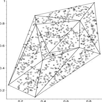
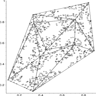
Figure 6: A realization of segregation (left) and association (right) for $|\mathcal{Y}|=10$, $J=13$, and $n=1000$.

Theorem 7: (Consistency) Let $J^{*}(\alpha,\varepsilon):=\left\lceil\Bigl{(}\frac{\sigma\cdot z_{\alpha}}{\mu-\overline{G}_{J}}\Bigr{)}^{2}\right\rceil$ where $\lceil\cdot\rceil$ is the ceiling function and $\varepsilon$-dependence is through $\overline{G}_{J}$ under a given alternative. Then the test against $H^{S}_{\varepsilon}$ which rejects for $S<z_{1-\alpha}$ is consistent for all $\varepsilon\in(0,\sqrt{3}/3)$ and $J\geq J^{*}(1-\alpha,\varepsilon)$, and the test against $H^{A}_{\varepsilon}$ which rejects for $S>z_{\alpha}$ is consistent for all $\varepsilon\in(0,\sqrt{3}/3)$ and $J\geq J^{*}(\alpha,\varepsilon)$.

Proof: Let $\varepsilon>0$. Under $H^{S}_{\varepsilon}$, $\gamma_{n,\varepsilon}(3/2)$ is degenerate in the limit as $n\rightarrow\infty$, which implies $\overline{G}_{J}$ is a constant a.s. In particular, for $\varepsilon\in(0,\sqrt{3}/4]$, $\overline{G}_{J}=2$ and for $\varepsilon\in(\sqrt{3}/4,\sqrt{3}/3)$, $\overline{G}_{J}=1$ a.s. as $n\rightarrow\infty$. Then the test statistic $S=\sqrt{J}(\overline{G}_{J}-\mu)/\sigma$ is a constant a.s. and $J\geq J^{*}(1-\alpha,\varepsilon)$ implies that $S<z_{1-\alpha}$ a.s. Hence consistency follows for segregation.

Under $H^{A}_{\varepsilon}$, as $n\rightarrow\infty$, $\overline{G}_{J}=3$ for all $\varepsilon\in(0,\sqrt{3}/3)$, a.s. Then $J\geq J^{*}(\alpha,\varepsilon)$ implies that $S>z_{\alpha}$ a.s., hence consistency follows for association. $\blacksquare$

6 Monte Carlo Power Analysis

In Figure 7, we observe empirically that even under mild segregation we obtain considerable separation between the kernel density estimates under null and segregation cases for moderate $J$ and $n$ values suggesting high power at $\alpha=.05$. A similar result is observed for association. With $J=13$ and $n=1000$, under $H_{0}$, the estimated significance level is $\widehat{\alpha}=.09$ relative to segregation, and $\widehat{\alpha}=.07$ relative to association. Under $H^{S}_{\sqrt{3}/8}$, the empirical power (using the asymptotic critical value) is $\widehat{\beta}=.97$, and under $H^{A}_{\sqrt{3}/21}$, $\widehat{\beta}=1.00$. With $J=30$ and $n=5000$, under $H_{0}$, the estimated significance level is $\widehat{\alpha}=.06$ relative to segregation, and $\widehat{\alpha}=.04$ relative to association. The empirical power is $\widehat{\beta}=1.00$ for both alternatives.

We also estimate the empirical power by using the empirical critical values. With $J=13$ and $n=1000$, under $H^{S}_{\sqrt{3}/8}$, the empirical power is $\widehat{\beta}_{mc}=.72$ at empirical level $\widehat{\alpha}_{mc}=.033$ and under $H^{A}_{\sqrt{3}/21}$ the empirical power is $\widehat{\beta}_{mc}=1.00$ at empirical level $\widehat{\alpha}_{mc}=.03$. With $J=30$ and $n=5000$, under $H^{S}_{\sqrt{3}/8}$, the empirical power is $\widehat{\beta}_{mc}=1.00$ at empirical level $\widehat{\alpha}_{mc}=.034$ and under $H^{A}_{\sqrt{3}/21}$ the empirical power is $\widehat{\beta}_{mc}=1.00$ at empirical level $\widehat{\alpha}_{mc}=.04$.

\psfrag{kernel density estimate}{ \Huge{\bf{kernel density estimate}}}\psfrag{relative density}{ \Huge{\bf{relative density}}}\includegraphics{GammaSegn1000.ps}

\psfrag{kernel density estimate}{ \Huge{\bf{kernel density estimate}}}\psfrag{relative density}{ \Huge{\bf{relative density}}}\includegraphics{GammaSegn5000.ps}

Figure 7: Two Monte Carlo experiments against the segregation alternatives $H^{S}_{\sqrt{3}/8}$ with $\delta=1/16$. Depicted are kernel density estimates of $\overline{G}_{J}$ for $J=13$ and $n=1000$ with $1000$ replicates (left) and $J=30$ and $n=5000$ with $1000$ replicates (right) under the null (solid) and alternative (dashed).

7 Extension to Higher Dimensions

The extension to $\mathbb{R}^{d}$ for $d>2$ is straightforward. Let $\mathcal{Y}=\{\mathsf{y}_{1},\mathsf{y}_{2},\cdots,\mathsf{y}_{d+1}\}$ be $d+1$ non-coplanar points. Denote the simplex formed by these $d+1$ points as $\mathfrak{S}(\mathcal{Y})$. (A simplex is the simplest polytope in $\mathbb{R}^{d}$ having $d+1$ vertices, $d\,(d+1)/2$ edges, and $d+1$ faces of dimension $(d-1)$.) For $r\in[1,\infty]$, define the $r$-factor proximity map as follows. Given a point $x$ in $\mathfrak{S}(\mathcal{Y})$, let $\mathsf{y}:=\arg\min_{\mathsf{y}\in\mathcal{Y}}\mbox{volume}(Q_{\mathsf{y}}(x))$ where $Q_{\mathsf{y}}(x)$ is the polytope with vertices being the $d\,(d+1)/2$ midpoints of the edges, the vertex $\mathsf{y}$ and $x$. That is, the vertex region for vertex $v$ is the polytope with vertices given by $v$ and the midpoints of the edges. Let $v(x)$ be the vertex in whose region $x$ falls. If $x$ falls on the boundary of two vertex regions, we assign $v(x)$ arbitrarily. Let $\varphi(x)$ be the face opposite to vertex $v(x)$, and $\eta(v(x),x)$ be the hyperplane parallel to $\varphi(x)$ which contains $x$. Let $d(v(x),\eta(v(x),x))$ be the (perpendicular) Euclidean distance from $v(x)$ to $\eta(v(x),x)$. For $r\in[1,\infty)$, let $\eta_{r}(v(x),x)$ be the hyperplane parallel to $\varphi(x)$ such that $d(v(x),\eta_{r}(v(x),x))=r\,d(v(x),\eta(v(x),x))$ and $d(\eta(v(x),x),\eta_{r}(v(x),x))<d(v(x),\eta_{r}(v(x),x))$. Let $\mathfrak{S}_{r}(x)$ be the polytope similar to and with the same orientation as $\mathfrak{S}$ having $v(x)$ as a vertex and $\eta_{r}(v(x),x)$ as the opposite face. Then the $r$-factor proximity region $N_{\mathcal{Y}}^{r}(x):=\mathfrak{S}_{r}(x)\cap\mathfrak{S}(\mathcal{Y})$. Also, let $\zeta_{j}(x)$ be the hyperplane such that $\zeta_{j}(x)\cap\mathfrak{S}(\mathcal{Y})\not=\emptyset$ and $r\,d(\mathsf{y}_{j},\zeta_{j}(x))=d(\mathsf{y}_{j},\eta(\mathsf{y}_{j},x))$ for $j=1,2,\ldots,d+1$. Then $\Gamma^{r}_{1}(x)=\cup_{j=1}^{d+1}(\Gamma^{r}_{1}(x)\cap R(\mathsf{y}_{j}))$ where $\Gamma^{r}_{1}(x)\cap R(\mathsf{y}_{j})=\{z\in R(\mathsf{y}_{j}):d(\mathsf{y}_{j},\eta(\mathsf{y}_{j},z))\geq d(\mathsf{y}_{j},\zeta_{j}(x)\}$, for $j=1,2,3$.

Theorem 1 generalizes, so that any simplex $\mathfrak{S}$ in $\mathbb{R}^{d}$ can be transformed into a regular polytope (with egdes being equal in length and faces being equal in volume) preserving uniformity. Delaunay triangulation becomes Delaunay tessellation in $\mathbb{R}^{d}$, provided that no more than $d+1$ points being cospherical (lying on the boundary of the same sphere). In particular, with $d=3$, the general simplex is a tetrahedron (4 vertices, 4 triangular faces and 6 edges), which can be mapped into a regular tetrahedron (4 faces are equilateral triangles) with vertices $(0,0,0),\,(1,0,0)\,(1/2,\sqrt{3}/2,0),\,(1/2,\sqrt{3}/6,\sqrt{6}/3)$. Let $\gamma_{n}(r,d)$ be the domination number for the extension to $\mathbb{R}^{d}$. Then it is easy to see that $\gamma_{n}(r,3)$ is nondegenerate as $n\rightarrow\infty$ for $r=4/3$, and otherwise degenerate. In $\mathbb{R}^{d}$, it can be seen that $\gamma_{n}(r,d)$ is nondegenerate in the limit only for $r=(d+1)/d$. Moreover, it can be shown that $\lim_{n\rightarrow\infty}P(2\leq\gamma_{n}((d+1)/d,d)\leq d+1)=1$, and we conjecture that

$$\lim_{n\rightarrow\infty}P(d\leq\gamma_{n}((d+1)/d,d)\leq d+1)=1.$$

7.1 Discussion

In this article we investigate the mathematical properties of a domination number method for the analysis of spatial point patterns.

The first proximity map related to $r$-factor proximity map, $N_{\mathcal{Y}}^{r}$, in literature is the spherical proximity map, $N_{S}(x):=B(x,r(x))$, (which is called CCCD in the literature, see [Priebe et al., 2001], [DeVinney et al., 2002], [Marchette and Priebe, 2003], [Priebe et al., 2003a], and [Priebe et al., 2003b]). A slight variation of $N_{S}$ is the arc-slice proximity map $N_{AS}(x):=B(x,r(x))\cap T(x)$ where $T(x)$ is the Delaunay cell that contains $x$ (see [Ceyhan and Priebe, 2003a]). Furthermore, Ceyhan and Priebe introduced the central similarity proximity map, $N_{CS}$, in [Ceyhan and Priebe, 2003a]. The $r$-factor proximity map, when compared to the others, has the advantages that the asymptotic distribution of the domination number $\gamma_{n}(r)$ is tractable (see Theorem 3). The distribution of the domination number of the proximity catch digraphs based on $N_{S}$ or $N_{AS}$ is not tractable, and that of $N_{CS}$ is an open problem. Furthermore, $N_{CS}$ and $N_{\mathcal{Y}}^{r}$ enjoy the geometry invariance property over triangles for uniform data. Moreover, while finding the exact minimum dominating sets is an NP-Hard problem for $N_{S}$, $N_{AS}$, and $N^{\tau}_{CS}$, the exact minimum dominating sets can be found in polynomial time for $N_{\mathcal{Y}}^{r}$. Additionally, $N_{AS}(x)$, $N_{\mathcal{Y}}^{r}(x)$, and $N^{\tau}_{CS}(x)$ are well defined only for $x\in C_{H}(\mathcal{Y})$, the convex hull of $\mathcal{Y}$, whereas $N_{S}(x)$ is well defined for all $x\in\mathbb{R}^{d}$.

The $N_{S}$ (the proximity map associated with CCCD) is used in classification in the literature, but not for testing spatial patterns between two or more classes. We develop a technique to test the patterns of segregation or association. There are many tests available for segregation and association in ecology literature. See [Dixon, 1994] for a survey on these tests and relevant references. Two of the most commonly used tests are Pielou’s $\chi^{2}$ test of independence and Ripley’s test based on $K(t)$ and $L(t)$ functions. However, the test we introduce here is not comparable to either of them. Our method deals with a slightly different type of data than most methods to examine spatial patterns. The sample size for one type of point (type $\mathcal{X}$ points) is much larger compared to the the other (type $\mathcal{Y}$ points).

The null hypothesis we consider is considerably more restrictive than current approaches, which can be used much more generally. The null hypothesis for testing segregation or association can be described in two slightly different forms ([Dixon, 1994]):

• complete spatial randomness, that is, each class is distributed randomly throughout the area of interest. It describes both the arrangement of the locations and the association between classes.

• random labeling of locations, which is less restrictive than spatial randomness, in the sense that arrangement of the locations can either be random or non-random.

Our test is closer to the former in this regard.

8 Appendix

Proof of Proposition 1

To prove Proposition 1, we show that the expected locus of the boundary of the $\Gamma_{1}$-region, $\partial(\Gamma_{1}^{r}(\mathcal{X}_{n}))$, goes to $\partial(\varsigma_{\mathcal{Y}}^{r})$ as $n\rightarrow\infty$ by showing that the expected loci of $X_{e_{j}}$ are $e_{j}$ for $j=1,2,3$. See [Ceyhan and Priebe, 2003b] for the details.

For sufficiently large $n$ and given $X_{e_{j}}=(x_{j},y_{j})$ for $j=1,2,3$,

$$A(\Gamma_{1}^{3/2}(\mathcal{X}_{n}))=\sqrt{3}/9(3\,{x_{2}}^{2}-6\,x_{2}+2\,\sqrt{3}y_{2}\,x_{2}-2\,\sqrt{3}y_{2}+{y_{2}}^{2}+3+{y_{3}}^{2}-2\,\sqrt{3}y_{3}\,x_{3}+3\,{x_{3}}^{2}+4\,{y_{1}}^{2}).$$

The asymptotically accurate joint pdf of $X_{e_{j}}$’s is

$$f_{3}(\zeta)=n(n-1)(n-2)\bigl{(}\sqrt{3}/36(-2\,\sqrt{3}y_{1}+\sqrt{3}y_{3}-3\,x_{3}+\sqrt{3}y_{2}+3\,x_{2})^{2}\bigr{)}^{n-3}/(\sqrt{3}/4)^{n}$$

with the support $D_{S}=\{\zeta=(x_{1},y_{1},x_{2},y_{2},x_{3},y_{3})\in\mathbb{R}^{6}:\;(x_{j},y_{j})\text{'s are distinct}\}.$ Then for sufficiently large $n$, $\mathbf{E}\,[A(\Gamma_{1}^{3/2}(\mathcal{X}_{n}))]\approx\int_{D_{S}}A(\Gamma_{1}^{3/2}(\mathcal{X}_{n}))f_{3}(\zeta)d\zeta,$ which goes to $0$ as $n\rightarrow\infty$ at the rate $O(n^{-2})$. See [Ceyhan and Priebe, 2003b] for the details.

Proof of Theorem 3

We know that $\gamma_{n}(r)\leq 3$ a.s. for all $r\in[1,\infty]$ and all $n$. First we show that $\lim_{n\rightarrow\infty}P(\gamma_{n}(3/2)>1)=1$.

Note that $P(\gamma_{n}(3/2)>1)=P(\mathcal{X}_{n}\cap\Gamma_{1}^{3/2}(\mathcal{X}_{n})=\emptyset)$. Then we find $P(\mathcal{X}_{n}\cap\Gamma_{1}^{3/2}(\mathcal{X}_{n})=\emptyset,\,E_{2}(n,\varepsilon))$ where $E_{2}(n,\varepsilon)$ is the event such that $\frac{2\varepsilon}{\sqrt{3}}\leq X_{1}\leq 1-\frac{2\varepsilon}{\sqrt{3}}$ and $0\leq Z_{1}\leq\varepsilon$, and $1/2\leq X_{2}\leq 1-\frac{2\varepsilon}{\sqrt{3}}$, $\sqrt{3}(1-X_{2})-\varepsilon\leq Z_{2}\leq\sqrt{3}(1-X_{2})$, and $\frac{2\varepsilon}{\sqrt{3}}\leq X_{3}\leq 1/2$, and $\sqrt{3}\,X_{3}-\varepsilon\leq Z_{3}\leq\sqrt{3}\,X_{3}$. First letting $n\rightarrow\infty$, then $\varepsilon\rightarrow 0$, yields the desired result. See [Ceyhan and Priebe, 2003b] for the details.

Next, $\lim_{n\rightarrow\infty}P(\gamma_{n}(3/2)\leq 2)=\lim_{n\rightarrow\infty}P(\gamma_{n}(3/2)=2)$, since $\lim_{n\rightarrow\infty}P(\gamma_{n}(3/2)=1)=0$. Let

$$Q_{j}:=\operatorname{argmin}_{x\in\mathcal{X}_{n}\cap R(\mathsf{y}_{j})}d(x,e_{j})=\operatorname{argmax}_{x\in\mathcal{X}_{n}\cap R(\mathsf{y}_{j})}d(\ell(\mathsf{y}_{j},x),e_{j})$$

where $e_{j}$ is the edge opposite vertex $\mathsf{y}_{j}$ for $j=1,2,3$ and let $q_{j}=(x_{j},y_{j})$ be the realization of $Q_{j}$ for $j=1,2,3$. Then $\gamma_{n}(3/2)\leq 2$ iff $\mathcal{X}_{n}\subset N_{\mathcal{Y}}^{3/2}(Q_{1})\cup N_{\mathcal{Y}}^{3/2}(Q_{2})$ or $\mathcal{X}_{n}\subset N_{\mathcal{Y}}^{3/2}(Q_{1})\cup N_{\mathcal{Y}}^{3/2}(Q_{3})$ or $\mathcal{X}_{n}\subset N_{\mathcal{Y}}^{3/2}(Q_{2})\cup N_{\mathcal{Y}}^{3/2}(Q_{3})$.

Let the events $E_{i,j}:=\mathcal{X}_{n}\subset N_{\mathcal{Y}}^{3/2}(Q_{i})\cup N_{\mathcal{Y}}^{3/2}(Q_{j})$ for $(i,j)=\{(1,2),(1,3),(2,3)\}$. Then

$$P(\gamma_{n}(3/2)\leq 2)=P(E_{1,2})+P(E_{1,3})+P(E_{2,3})-P(E_{1,2}\cap E_{1,3})-P(E_{1,2}\cap E_{2,3})-P(E_{1,3}\cap E_{2,3})+P(E_{1,2}\cap E_{1,3}\cap E_{2,3}).$$

By symmetry, $P(E_{1,2})=P(E_{1,3})=P(E_{2,3})$ and $P(E_{1,2}\cap E_{1,3})=P(E_{1,2}\cap E_{2,3})=P(E_{1,3}\cap E_{2,3})$. Hence

$$P(\gamma_{n}(3/2)\leq 2)=3\,\Bigl{[}P(E_{1,2})-P(E_{1,2}\cap E_{1,3})\Bigr{]}+P(E_{1,2}\cap E_{1,3}\cap E_{2,3}).$$

We find $P(E_{1,2})$, by finding the asymptotically accurate joint pdf of $Q_{1},\,Q_{2}$. Let $T(Q_{j})$ be the triangle formed by the median lines at $\mathsf{y}_{k}$ and $\mathsf{y}_{l}$ for $k,l\not=j$ and $\ell(\mathsf{y}_{j},Q_{j})$, and let $\varepsilon>0$ be small enough such that $T(Q_{j})\subset R(\mathsf{y}_{j})$, for $j=1,2,3$. Then the asymptotically accurate joint pdf of $Q_{1},\,Q_{2}$ is

$$f_{1,2}(x_{1},y_{1},x_{2},y_{2})=n\,(n-1)\,\frac{1}{A(T(\mathcal{Y}))^{2}}\left(\frac{A(T(\mathcal{Y}))-A(T(q_{1}))-A(T(q_{2}))}{A(T(\mathcal{Y}))}\right)^{n-2}$$

where $A(T(q_{1}))=\sqrt{3}/36\left(-2\,\sqrt{3}+3\,y_{1}+3\,\sqrt{3}x_{1}\right)^{2}$ and $A(T(q_{2}))=\sqrt{3}/36\left(-3\,y_{2}-\sqrt{3}+3\,\sqrt{3}x_{2}\right)^{2}$ with domain $D_{I}=\{(x_{1},y_{1})\in R(\mathsf{y}_{1}):\;y_{1}\geq-\frac{\sqrt{3}}{3}\,+\sqrt{3}x_{1}+\sqrt{3}\varepsilon,\;(x_{2},y_{2})\in R(\mathsf{y}_{2}):\;y_{2}\leq-\frac{\sqrt{3}}{3}\,+\sqrt{3}x_{2}-\sqrt{3}\,\varepsilon\}$ with $\varepsilon>0$ be small enough such that $T(Q_{j})\subset R(\mathsf{y}_{j})$, for $j=1,2,3$.

Then $P(E_{1,2})\approx.4126$ (which is found numerically). See [Ceyhan and Priebe, 2003b] for the details.

Similarly we find $P(E_{1,2}\cap E_{1,3})$, by finding the joint pdf of $Q_{1},\,Q_{2},\,Q_{3}$, where $T(q_{3})$ is the triangle with vertices $\frac{1}{3}\,(\sqrt{3}-3\,y_{3})\sqrt{3},y_{3}),\,(1/2,\sqrt{3}/6),(\sqrt{3}y_{3},y_{3})$. Then the asymptotically accurate joint pdf of $Q_{1},\,Q_{2},\,Q_{3}$ is

$$f_{123}(x_{1},y_{1},x_{2},y_{2},x_{3},y_{3})=n\,(n-1)\,(n-2)\,\frac{1}{A(T(\mathcal{Y}))^{3}}\left(\frac{A(T(\mathcal{Y}))-A(T(q_{1}))-A(T(q_{2}))-A(T(q_{3}))}{A(T(\mathcal{Y}))}\right)^{n-3}$$

where $A(T(q_{3}))=\frac{\sqrt{3}}{36}\,(-\sqrt{3}+6\,y_{3})^{2}$ with domain $D_{I}=\{(x_{1},y_{1})\in R(\mathsf{y}_{1}):\;y_{1}\geq-\frac{\sqrt{3}}{3}\,+\sqrt{3}x_{1}+\sqrt{3}\,\varepsilon,\;(x_{2},y_{2})\in R(\mathsf{y}_{2}):\;y_{2}\geq-\frac{\sqrt{3}}{3}\,+\sqrt{3}x_{2}-\sqrt{3}\,\varepsilon,\;(x_{3},y_{3})\in R(\mathsf{y}_{3}):\;y_{3}\leq\frac{\sqrt{3}}{6}+\varepsilon\}$.

Then $P(E_{1,2}\cap E_{1,3})\approx.2009$ (see [Ceyhan and Priebe, 2003b] for the details.)

Likewise, we find $P(E_{1,2}\cap E_{1,3}\cap E_{2,3})\approx.1062$ (see [Ceyhan and Priebe, 2003b] for the details.)

Hence we get $\lim_{n\rightarrow\infty}P(\gamma(\mathcal{X}_{n},N_{\mathcal{Y}}^{3/2})=2)\approx.7413$, and $\lim_{n\rightarrow\infty}P(\gamma(\mathcal{X}_{n},N_{\mathcal{Y}}^{3/2})=3)\approx.2587$.

References

- [Ceyhan and Priebe, 2003a] Ceyhan, E. and Priebe, C. (2003a). Central similarity proximity maps in Delaunay tessellations. In Proceedings of the Joint Statistical Meeting, Statistical Computing Section, American Statistical Association.
- [Ceyhan and Priebe, 2003b] Ceyhan, E. and Priebe, C. (2003b). The use of domination number of a random proximity catch digraph for testing segregation/association. Technical Report 642, Department of Applied Mathematics and Statistics, Johns Hopkins University, Baltimore, MD 21218-2682. submitted for publication.
- [Coomes et al., 1999] Coomes, D. A., Rees, M., and L., T. (1999). Identifying aggregation and association in fully mapped spatial data. Ecology, 80:554–565.
- [DeVinney et al., 2002] DeVinney, J., Priebe, C. E., Marchette, D. J., and Socolinsky, D. (2002). Random walks and catch digraphs in classification. http://www.galaxy.gmu.edu/interface/I02/I2002Proceedings/DeVinneyJason/%%****␣AsyGamArchive.tex␣Line␣800␣****DeVinneyJason.paper.pdf. Computing Science and Statistics, Vol. 34.
- [Dixon, 1994] Dixon, P. M. (1994). Testing spatial segregation using a nearest-neighbor contingency table. Ecology, 75(7):1940–1948.
- [Gotelli and Graves, 1996] Gotelli, N. J. and Graves, G. R. (1996). Null Models in Ecology. Smithsonian Institution Press.
- [Marchette and Priebe, 2003] Marchette, D. J. and Priebe, C. E. (2003). Characterizing the scale dimension of a high dimensional classification problem. Pattern Recognition, 36(1):45–60.
- [Priebe et al., 2001] Priebe, C. E., DeVinney, J. G., and Marchette, D. J. (2001). On the distribution of the domination number of random class catch cover digraphs. Statistics and Probability Letters, 55:239–246.
- [Priebe et al., 2003a] Priebe, C. E., Marchette, D. J., DeVinney, J., and Socolinsky, D. (2003a). Classification using class cover catch digraphs. Journal of Classification, 20(1):3–23.
- [Priebe et al., 2003b] Priebe, C. E., Solka, J. L., Marchette, D. J., and Clark, B. T. (2003b). Class cover catch digraphs for latent class discovery in gene expression monitoring by DNA microarrays. Computational Statistics and Data Analysis on Visualization, 43-4:621–632.
- [West, 2001] West, D. B. (2001). Introduction to Graph Theory, 2nd ed. Prentice Hall, NJ.