Time–space white noise eliminates global solutions in reaction diffusion equations

Abstract.

We prove that perturbing the reaction–diffusion equation $u_{t}=u_{xx}+(u_{+})^{p}$ ($p>1$), with time–space white noise produces that solutions explodes with probability one for every initial datum, opposite to the deterministic model where a positive stationary solution exists.

1. Introduction

In this paper we study the following parabolic SPDE with additive noise

(1.1) $$u_{t}=u_{xx}+f(u)+\sigma\dot{W}(x,t),$$

in an interval $(0,1)$, complemented with homogeneous Dirichlet boundary conditions. Here $W$ is a $2-$dimensional Brownian sheet, $\sigma$ is a positive parameter and $f$ is a locally Lipschitz real function.

We restrict ourselves to one space dimension since for higher dimensions the solution to (1.1) (if it exists) it is not expected to be a function valued process and have to be understood in a distributional sense. But in this case there is no natural way to define $f(u)$, see [17] for more on this.

Semilinear parabolic equations like (1.1) arises in the phenomenological approach to such different phenomena as the diffusion of a fluid in a porous medium, transport in a semiconductor, chemical reactions with possibility of spatial diffusion, population dynamics, chemotaxis in biological systems, etc. In all these cases, due to the phenomenological approximate character of the equations, it is of interest to test how the description changes under the effect of stochastic perturbation.

Equation (1.1) with $f$ globally Lipschitz has been widely studied (see [17, 19]), in this case global solutions exist with probability one. However, when $f$ is just locally Lipschitz, typically $f(s)\sim s^{p}$ with $p>1$ or $f(s)\sim{\rm e}^{s}$, there are practically no results on this problem. Using standard approximation arguments one can easily prove the existence of local in time solutions but it does not follow from that proof the behavior of the maximal time of existence.

On the other hand, the deterministic case (i.e. $\sigma=0$) is very well understood. One problem that has drawn the attention to the PDE community is the appearance of singularities in finite time, no matter how smooth the initial data is. This phenomena is known as blow-up. What happens is that solutions go to infinity in finite time, that is, there exists a time $T<\infty$ such that

$$\lim_{t\nearrow T}\|u(\cdot,t)\|_{\infty}=\infty.$$

A well known condition on the nonlinear term $f$ that assures this phenomena is when $f$ is a nonnegative convex function with

$$\int^{\infty}\frac{1}{f}<\infty.$$

For a general reference of these facts and much more on blow-up problems, see the book [18] and the surveys [1, 6].

For a large class of nonlinearities $f$, such as the ones mentioned above, problem (1.1) with $\sigma=0$ admits a stationary positive solution $v$ and hence, since the comparison principle holds for this equation, for every initial datum $u_{0}\leq v$ the solution to (1.1) is global in time.

It is well known (see [6, 18]) that the appearance of blow-up persists under (small) regular perturbations. On the other hand, regular perturbations of (1.1) with $\sigma=0$ admit global in time solutions. Summarizing, the existence of global in time/blowing up solutions for this problem with $\sigma=0$ is stable under small regular perturbations. Hence it is of interest to test how this phenomena is affected by stochastic perturbations.

Surprisingly, the situation changes for $\sigma>0$. We prove that, in this case, there is no global in time solution. In fact, for every initial nonnegative datum $u_{0}$, the solution to (1.1) blows up with probability one.

Stochastic partial differential equations with blow-up has been considered by C. Mueller in [14, 15] and C. Mueller and R. Sowers in [16]. In those papers, a linear drift with a nonlinear multiplicative noise is considered and the explosion is due to this latter term.

A similar result, but in some sense in the opposite direction, was proved by Mao, Marion and Renshaw in [13]. There, the authors prove for a system of ODEs that arise in population dynamics and that have blow-up solutions, that perturbing some coefficients of the system with a small Brownian noise, global solutions a.s. are obtained for every initial data.

In our problem, a common way to interpret the asymptotic behavior of $u$ is the following: consider first the deterministic case $\sigma=0$. In this case there is some kind of competition between the diffusion, which diffuses the zero boundary condition to the interior of the domain and the nonlinear source $f(u)$ that induces $u$ to grow very fast.

Again in the deterministic case, it was proved in [4] that for small initial datum $u_{0}$, $u\to 0$ as $t\to+\infty$, while for $u_{0}$ large, there exists a finite time $T$, such that $\|u(\cdot,t)\|_{\infty}\nearrow+\infty$ as $t\nearrow T$. More precisely, it is proved that for every data $u_{0}$, there exists a critical parameter $\lambda^{*}$ such that if we solve the PDE with initial data $\lambda u_{0}$, for $\lambda<\lambda^{*}$ the solution converges to $0$ uniformly, for $\lambda>\lambda^{*}$ the solution blows-up in finite time and for $\lambda=\lambda^{*}$ the solution converges uniformly to the unique positive steady state.

For small noise $\sigma\ll 1$ one could expect a similar behavior. Of course we can not expect convergence to the zero solution as $t\to\infty$ since in this case $v\equiv 0$ is not invariant for (1.1), but it is reasonable to suspect the existence of an invariant measure close to the zero solution of the deterministic PDE and convergence to this invariant measure for small initial datum as $t\to\infty$.

However, that is not the case. We prove in Section 3 that for every initial datum $u_{0}$ solutions to (1.1) blow-up in finite time with probability one.

Numerical simulations, as well as heuristical arguments, suggest that, for small initial data $u_{0}$, metastability could be taking place in this case. Metastability appears here since, while the noise remains relatively small, the solution stays in the domain of attraction of the zero solution of the deterministic problem. But, as soon as the noise becomes large, the solution escapes this domain of attraction and hence the reaction term begins to dominate and pushes forward the solution until ultimately explosion cannot be prevented by the action of the noise.

Organization of the paper

The paper is organized as follows. In Section 2 we give the rigorous meaning of (1.1) and give the references where the foundations for the study of this kind of equation were laid. Section 3 deals with the proof of the main result of this paper: the explosion of the solutions of (1.1). In Section 4 we propose a semidiscrete scheme in order to approximate the solutions to (1.1). We prove that the numerical approximations also explode with probability one and that they converge a.s., in time intervals where the continuous solution remains bounded. Finally, in Section 5 we show some numerical simulations for this equation.

2. Formulation of the problem

We begin this section discussing the rigorous meaning of (1.1), the references for this being [2, 11, 17, 19]. There are two alternatives: the integral and the weak formulation as described in [2, 17, 19]. The last being more suitable for our purposes. Both formulations are equivalent as is shown in [19].

Let $(\Omega,\mathcal{F},(\mathcal{F}_{t})_{t\geq 0},\mathbb{P})$ be a probability space equipped with a filtration $(\mathcal{F}_{t})_{t\geq 0}$ which is supposed to be right continuous and such that $\mathcal{F}_{0}$ contains all the $\mathbb{P}-$null sets of $\mathcal{F}$. We are given a space-time white noise on ${\mathbb{R}}_{+}\times[0,1]$ defined on $(\Omega,\mathcal{F},(\mathcal{F}_{t})_{t\geq 0},\mathbb{P})$ and $u_{0}\in C_{0}([0,1])$.

Assume for a moment that $f$ is globally Lipschitz, multiply (1.1) by a test function $\varphi\in C^{2}((0,1))\cap C_{0}([0,1])$ and integrate to obtain

(2.1) $$\int_{0}^{1} u(x,t)\varphi(x)\,dx-\int_{0}^{1}u_{0}(x)\varphi(x)\,dx=$$

$$\int_{0}^{t}\int_{0}^{1}u(s,x)\varphi_{xx}(x)\,dx\,ds+\int_{0}^{t}\int_{0}^{1}f(u(s,x))\varphi(x)\,dx\,ds$$

$$+\sigma\int_{0}^{t}\int_{0}^{1}\varphi(x)\,dW(x,s).$$

Alternatively, the integral formulation of the problem is constructed by means of the function $G$, the fundamental solution of the heat equation for the domain $(0,1)$.

$$u(x,t)- \int_{0}^{1}G_{t}(x,y)u_{0}(y)\,dy=$$

$$\int_{0}^{t}\int_{0}^{1}G_{t-s}(x,y)f(u(y,s))\,dyds+\sigma\int_{0}^{t}\int_{0}^{1}G_{t-s}(x,y)dW(y,s).$$

As a solution to (1.1) we understand an $\mathcal{F}_{t}-$adapted process with values in $C_{0}([0,1])$ that verifies (2.1) for every $\varphi\in C^{\infty}((0,1))\cap C_{0}([0,1])$.

In [2, 19] it is proved that there exists a unique solution to this problem and that the integral and weak formulations are equivalent.

For $f$ locally Lipschitz globally defined solutions do not exist in general. Nevertheless, existence of local in time solutions is proved by standard arguments: consider for each $n\in{\mathbb{N}}$ the globally Lipschitz function $f_{n}(x)=f(-n)\mathbf{1}_{(-\infty,-n]}+f(x)\mathbf{1}_{(-n,n)}+f(n)\mathbf{1}_{[n,+\infty)}$ and $u^{n}$, the unique solution of (1.1) with $f$ replaced by $f_{n}$. Let $T_{n}$ be the first time at which $\|u^{n}(\cdot,t)\|_{\infty}$ reaches the value $n$. Then $(T_{n})_{n}$ is an increasing sequence of stopping times and we define the maximal existence time of (1.1) as $T:=\lim T_{n}$. It is easy to see that $u^{n+1}\mathbf{1}_{\{t<T_{n}\}}=u^{n}\mathbf{1}_{\{t<T_{n}\}}$ a.s. and hence there exist the limit $u(x,t)=\lim u^{n}(x,t)$ for $t<T$ which verifies

(2.2) $$\int_{0}^{1} u(x,t\wedge T)\varphi(x)\,dx-\int_{0}^{1}u_{0}(x)\varphi(x)\,dx=$$

$$\int_{0}^{t\wedge T}\int_{0}^{1}u(s,x)\varphi_{xx}(x)\,dx\,ds+\int_{0}^{t\wedge T}\int_{0}^{1}f(u(s,x))\varphi(x)\,dx\,ds$$

$$+\sigma\int_{0}^{t\wedge T}\int_{0}^{1}\varphi(x)\,dW(x,s).$$

So we say that $u$ solves (1.1) up to the explosion time $T$. We also say that $u$ blows up in finite time if $\mathbb{P}(T<\infty)>0$. Observe that if $T(\omega)<\infty$ then

$$\lim_{t\nearrow T(\omega)}\|u(\cdot,t,\omega)\|_{\infty}=\infty.$$

3. Explosions

In this section, we show that equation (1.1) blows-up in finite time with probability one for every initial datum $u_{0}\in C_{0}([0,1])$. Hereafter we assume that $f$ is a nonnegative convex function, hence locally Lipschitz. Moreover we assume that $\int^{\infty}1/f<\infty$.

In order to prove the blow-up of $u$, we define the function

$$\Phi(t):=\int_{0}^{1}\phi(x)u(x,t)\,dx.$$

Here $\phi(x)>0$ is the normalized first eigenfunction of the Dirichlet Laplacian in $(0,1)$. That is, $\phi(x)=\tfrac{\pi}{2}\sin(\pi x)$ and hence we can use it as a test function in (2.1) to obtain

$$\Phi(t)-\Phi(0)= -\lambda_{1}\int_{0}^{t}\Phi(s)\,ds+\int_{0}^{t}\int_{0}^{1}\phi(x)f(u(x,s))\,dxds$$

$$+\sigma\int_{0}^{t}\int_{0}^{1}\phi(x)\,dW(x,s).$$

We denote by $z_{0}:=\Phi(0)=\int_{0}^{1}\phi(x)u_{0}(x)\,dx$.

Now, as $f$ is convex, by Jensen’s inequality, we get

$$\int_{0}^{1}\phi(x)f(u(x,s))\,dx\geq f\Big{(}\int_{0}^{1}\phi(x)u(x,s)\,dx\Big{)}=f(\Phi(s)).$$

Moreover, since $\phi$ is a positive function with $L^{1}-$norm equal to 1, it is easy to see that

$$B(t):=\frac{\sqrt{8}}{\pi}\int_{0}^{t}\int_{0}^{1}\phi(x)\,dW(x,s),$$

is a standard Brownian motion.

Combining all these facts, we obtain that $\Phi$ verifies the (one dimensional) stochastic differential inequality

$$d\Phi(t)\geq\big{(}-\lambda_{1}\Phi(t)+f(\Phi(t))\big{)}\,dt+\frac{\pi}{\sqrt{8}}\sigma dB(t).$$

Define $z(t)$ to be the one-dimensional process that verifies

$$dz=(-\lambda_{1}z+f(z))\,dt+\sigma dB,$$

with initial condition $z(0)=z_{0}$. Then, $e(t)=\Phi(t)-z(t)$ verifies

$$de\geq\Big{(}-\lambda_{1}e+\frac{f(\Phi)-f(z)}{\Phi-z}e\Big{)}\,dt.$$

Observe that $e$ verifies a deterministic differential inequality. Hence, as $e(0)=0$ it is easy to check that $e(t)\geq 0$ as long as it is defined.

Therefore, $\Phi(t)\geq z(t)$ as long as $\Phi$ is defined.

The following lemma proves that $z$ explodes with probability one.

Lemma 3.1.

Let $z$ be the solution of

(3.1) $$dz=(-\lambda_{1}z+f(z))\,dt+\sigma dB,\qquad z(0)=0.$$

Then $z$ explodes in finite time with probability one.

Proof.

The proof is just an application of the Feller Test for explosions ([12], Chapter 5). Using the same notation as in [12] we obtain the scale function for (3.1) to be

$$p(x)=\int_{0}^{x}\exp\left(-\frac{2}{\sigma^{2}}\int_{0}^{s}b(\xi)\,d\xi\right)\,ds$$

Here $b(\xi)=-\lambda_{1}\xi+f(\xi)$.

It is easy to see that, as $\int^{\infty}1/f<\infty$,

$$p(-\infty)=-\infty,\qquad p(+\infty)<+\infty,$$

and hence the Feller Test implies that, if $S$ is the explosion time of $z$, we get

$$\mathbb{P}\left(\lim_{t\nearrow S}z(t)=+\infty\right)=1$$

To prove that $\mathbb{P}(S<+\infty)=1$ we have to consider the function

$$v(x)=2\int_{0}^{x}\frac{p(x)-p(y)}{\sigma^{2}p(y)}\,dy.$$

The behavior of $v$ at $+\infty$ is given by $1/f$ and hence $v(+\infty)<+\infty$, which implies that

$$\mathbb{P}(S<\infty)=1.$$

This completes the proof. ∎

These facts all together, imply that there exists a (random) time $T=T(\omega)<\infty$ a.s. such that

$$\lim_{t\nearrow T}\|u(\cdot,t)\|_{\infty}=\infty\quad\text{a.s.}$$

So we have proved the following Theorem.

Theorem 3.2.

Let $f$ be a nonnegative, convex function such that

$$\int^{\infty}\frac{1}{f}\,<\infty.$$

Then, for every nonnegative initial datum $u_{0}\geq 0$ the solution $u$ to (1.1) blows-up in finite (random) time $T$ with

$$\mathbb{P}^{u_{0}}(T<\infty)=1.$$

4. Numerical approximations

In this section we introduce a numerical scheme in order to compute solutions to problem (1.1). We discretize the space variable with second order finite differences in a uniform mesh of size $h=1/n$. That is, for $x:=i/n,i=1,2,\dots,n-1$ the process $u^{n}(t,i/n)=u_{i}(t)$ is defined as the solution of the system of stochastic differential equations

(4.1) $$du_{i}=\frac{1}{h^{2}}(u_{i+1}-2u_{i}+u_{i-1})dt+f(u_{i})\,dt+\frac{\sigma}{\sqrt{h}}\,dw_{i},\quad 2\leq i\leq n-1,$$

accompanied with the boundary conditions $u_{1}(t)=u_{n}(t)=0$, $u_{i}(0)=u_{0}(ih)$, $1\leq i\leq n$. The Brownian motions $w_{i}$ are obtained by space integration of the Brownian sheet in the interval $[ih,(i+1)h)$.

Equivalently, this can be written as

$$dU=(-AU+f(U))\,dt+\frac{\sigma}{\sqrt{h}}\,dW,U(0)=U^{0}.$$

Where $U(t)=(u_{1}(t),\dots,u_{n}(t))$, $-A$ is the discrete laplacian, $f(U)$ in understood componentwise (i.e. $f(U)_{i}=f(u_{i}))$, $dW=(dw_{1},\dots,dw_{n})$ and $(U^{0})_{i}=u_{0}(ih)$.

With the same techniques of Theorem 3.2 it can be proved that solutions to this system of SDEs explodes in finite time with probability one.

We extend $u^{n}(t,\cdot)$ to the whole interval $[0,1]$ by linear interpolation in the space variable for each $t$.

Concerning the explosions of this system of SDEs we have the following

Theorem 4.1.

Let $f$ be a nonnegative, convex function such that

$$\int^{\infty}\frac{1}{f}\,<\infty.$$

Then, for every nonnegative initial datum $U^{0}\geq 0$ the solution $U$ to (4.1) blows-up in finite (random) time $T^{n}$ with

$$\mathbb{P}^{U^{0}}(T^{n}<\infty)=1.$$

Proof.

The proof uses the same technique of that of Theorem 3.2. Since $A$ is a symmetric positive definite matrix, we have a sequence of positive eigenvalues of $A$, $0<\lambda^{n}_{1}\leq\dots\leq\lambda_{n}^{n}$. Let $\phi^{n}$ the eigenvector associated to $\lambda^{n}_{1}$. It is easy to see that one can tale $\phi^{n}$ such that $\phi^{n}_{j}\geq 0$ for every $j$, and we assume that it is normalized such that $\sum_{i=1}^{n}h\phi_{i}^{n}=1$. Now, consider the function

$$\Phi^{n}(t)=\sum_{i=1}^{n}h\phi^{n}_{i}u_{i}(t).$$

Proceeding as in the proof of Theorem 3.2 we get that $\Phi^{n}$ verifies

$$d\Phi^{n}(t)\geq(-\lambda^{n}_{1}\Phi^{n}(t)+f(\Phi^{n}(t)))\,dt+\sigma_{n}dB(t),$$

where $B$ is a standard Brownian motion and $\sigma_{n}\to\sigma\pi/\sqrt{8}$. The rest of the proof follows by Lemma 3.1 as in Theorem 3.2. ∎

Now we turn to the problem of convergence of the approximations. In [10] convergence of this numerical scheme for globally Lipschitz reactions is proved

Theorem 4.2 (Gyöngy, [10] Theorem 3.1).

Assume $f$ is globally Lipschitz and $u_{0}\in C^{3}([0,1])$. Then

1. For every $p\geq 1$ and for every $T>0$ there exists a constant $K=K(p,T)$ such that

   $$\sup_{0\leq t\leq T}\sup_{x\in[0,1]}\mathbb{E}(|u^{n}(t,x)-u(t,x)|^{2p})\leq\frac{K}{n^{p}}.$$

2. $u^{n}(t,x)$ converges to $u(t,x)$ uniformly in $[0,T]\times[0,1]$ almost surely as $n\to\infty$.

Based on this theorem we can prove that even when $f$ is just locally Lipschitz, convergence holds but just in (stochastic) time intervals where the solution remains bounded. Observe that a better convergence result is not expected. Since the explosion times of $u$ and $u^{n}$ in general are different, then $\|u^{n}(t,\cdot)-u(t,\cdot)\|_{\infty}$ is unbounded in intervals of the form $[0,\tau]$ with $\tau$ close to the minimum of the explosion times. To state the convergence result we define the following stopping times. Let $M>0$ and consider $R_{M}:=\inf\{t>0,\|u(t,\cdot)\|_{L^{\infty}([0,1])}\geq M\}$ and $R^{n}_{M}:=\inf\{t>0,\|u^{n}(t,\cdot)\|_{L^{\infty}([0,1])}\geq M\}$

Theorem 4.3.

Assume $f$ is a nonnegative convex function with $\int\tfrac{1}{f}<\infty$. Let $u$ be the solution to (1.1) and $u^{n}$ its numerical approximation given by (4.1). Then

1. For every $p\geq 1$ and for every $T>0$ there exists a constant $K=K(p,T)$ such that

   $$\sup_{0\leq t\leq T}\sup_{x\in[0,1]}\mathbb{E}(|u^{n}(t,x)-u(t,x)|^{2p}\mathbf{1}_{\{t\leq R_{M}\wedge R^{n}_{M}\}})\leq\frac{K}{n^{p}}.$$

2. For every $M\geq 0$ $\|u^{n}-u\|_{L^{\infty}([0,T\wedge R_{M}]\times[0,1])}$ converges to zero almost surely as $n\to\infty$.

Remark 4.1.

Observe that statement (2) does not make assumptions on the numerical approximations $u^{n}$.

Proof.

First, we truncate the $f$ to get a globally Lipschitz function, bounded and that coincides with the original $f$ for values of $s$ with $|s|\leq M$. i.e. we consider

$$f_{M}(s) =\left\{\begin{array}[]{ll}f(s)&\mbox{if }|s|\leq M\\ f(M)&\mbox{if }s\geq M\\ f(-M)&\mbox{if }s\leq-M,\end{array}\right.$$

Let $w$ and $w^{n}$ be the solutions of (1.1) and (4.1) with $f$ replaced by $f_{M}$ respectively.

From Theorem 4.2,

$$\sup_{0\leq t\leq T}\sup_{x\in[0,1]}\mathbb{E}(|w^{n}(t,x)-w(t,x)|^{2p})\leq\frac{K}{n^{p}},$$

From the uniqueness of solutions of(1.1) and (4.1) up to the stopping time $R_{M}\wedge R_{M}^{n}$, we have that almos surely, if $t\leq R_{M}\wedge R_{M}^{n}$ then $u(t,x)=w(t,x)$ and $u^{n}(t,x)=w^{n}(t,x)$, hence

$$\sup_{0\leq t\leq T}\sup_{x\in[0,1]} \mathbb{E}(|u^{n}(t,x)-u(t,x)|^{2p}\mathbf{1}_{\{t\leq R_{M}\wedge R^{n}_{M}\}})=$$

$$\sup_{0\leq t\leq T}\sup_{x\in[0,1]}\mathbb{E}(|w^{n}(t,x)-w(t,x)|^{2p}\mathbf{1}_{\{t\leq R_{M}\wedge R^{n}_{M}\}})\leq$$

$$\sup_{0\leq t\leq T}\sup_{x\in[0,1]}\mathbb{E}(|w^{n}(t,x)-w(t,x)|^{2p})\leq\frac{K}{n^{p}}.$$

This proves (1). To prove (2) observe that since $w^{n}\to w$ almost surely and uniformly in $[0,T]\times[0,1]$ we have that for every $\varepsilon>0$ and $0\leq t\leq R_{M}$, $\|w^{n}(t,\cdot)\|_{\infty}\leq M+\varepsilon$ if $n$ is large enough. That means that $\liminf R_{M}^{n}\geq R_{M}$ and hence $R_{M}\wedge R_{M}^{n}\to R_{M}$. That is the reason we can get rid of $R_{M}^{n}$. So we have

$$0= \lim_{n\to\infty}\|w^{n}-w\|_{L^{\infty}([0,T]\times[0,1])}$$

$$\geq \lim_{n\to\infty}\|(w^{n}-w)\mathbf{1}_{\{t\leq R_{M-1}\wedge R^{n}_{M}\}}\|_{L^{\infty}([0,T]\times[0,1])}$$

$$= \lim_{n\to\infty}\|(u^{n}-u)\mathbf{1}_{\{t\leq R_{M-1}\wedge R^{n}_{M}\}}\|_{L^{\infty}([0,T]\times[0,1])}$$

$$\geq \lim_{n\to\infty}\|(u^{n}-u)\mathbf{1}_{\{t\leq R_{M-1}\}}\|_{L^{\infty}([0,T]\times[0,1])}$$

$$= \lim_{n\to\infty}\|u^{n}-u\|_{L^{\infty}([0,T\wedge R_{M-1}]\times[0,1])}.$$

Since $M$ is an arbitrary constant, this proves (2). ∎

Remark 4.2.

In order to compute an approximate solution this discretization in not enough, now we need to discretize the time variable but this is much simpler since now we are dealing with a SDE instead of a SPDE. The time discretization of (4.1) can be handled as in [5].

5. Numerical experiments

In this section we show some numerical simulations of (1.1). We perform all the simulations with the reaction $f(u)=(u_{+})^{2}$, $\sigma=6.36$ and initial datum $u_{0}\equiv 0$.

$$\begin{array}[]{ccc}\includegraphics[width=113.81102pt]{s45t1.000.eps}&\includegraphics[width=113.81102pt]{s45t50.000.eps}&\includegraphics[width=113.81102pt]{s45t72.0202.eps}\\[-6.0pt] \scriptstyle t=1&\scriptstyle t=50&\scriptstyle t=72.0202\\ \includegraphics[width=113.81102pt]{s45t72.4202.eps}&\includegraphics[width=113.81102pt]{s45t72.4802.eps}&\includegraphics[width=113.81102pt]{s45t72.5002.eps}\\[-6.0pt] \scriptstyle t=72.4202&\scriptstyle t=72.4802&\scriptstyle t=72.5002\\ \includegraphics[width=113.81102pt]{s45t72.5012.eps}&\includegraphics[width=113.81102pt]{s45t72.5068.eps}&\includegraphics[width=113.81102pt]{s45t72.5076.eps}\\[-6.0pt] \scriptstyle t=72.5012&\scriptstyle t=72.5068&\scriptstyle t=72.5076\end{array}$$

Figure 1. Profiles of a sample solution at different times.

Snapshot	Time	$\|u(\cdot,t,\omega)\|_{\infty}$
1	1.0000	5.6159
2	50.0000	3.3863
3	72.0202	15.5104
4	72.4202	18.2885
5	72.4802	38.5848
6	72.5002	82.8705
7	72.5012	203.0799
8	72.5068	$2.2695\times 10^{3}$
9	72.5076	$1.8128\times 10^{12}$

Table 1. The maximum of the solution at differen times

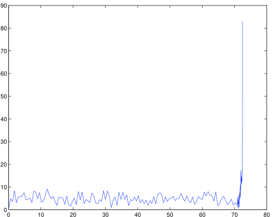
Figure 2. The evolution of the maximum of a sample solution with initial data $u_{0}\equiv 0$

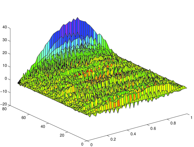
Figure 3. The graph of a sample solution with initial datum $u_{0}\equiv 0$

$$\begin{array}[]{cc}\includegraphics[width=170.71652pt]{density.eps}&\includegraphics[width=170.71652pt]{boxplot}\end{array}$$

Figure 4. The kernel density estimator of the explosion time for $\sigma=6.36$ and the corresponding box–plot.

To perform the simulations we use the numerical scheme introduced in Section 4, that is we discretize the space variable with second order finite differences in a uniform mesh of size $h=0.02$ (i.e.: $n=50$ nodes). With this discretization we obtain a system of SDE that reads

$$du_{i}=\frac{1}{h^{2}}(u_{i+1}-2u_{i}+u_{i-1})dt+f(u_{i})\,dt+\frac{\sigma}{\sqrt{h}}\,dw_{i},\quad 2\leq i\leq n-1,$$

accompanied with the boundary conditions $u_{1}=u_{n}=0$, $u_{i}(0)=u_{0}(ih)$, $1\leq i\leq n$. The Brownian motions $w_{i}$ are obtained by space integration of the Brownian sheet in the interval $[(i-1/2)h,(i+1/2)h)$.

To integrate this system we use an adaptive procedure similar to the one developed in [5] for the one dimensional case. Here we adapt the time step as in that work replacing the value of the solution (which is a real number) by the $L^{1}-$norm of $u^{j}$, as is done in [9] for the deterministic case. More precisely, the totally discrete scheme reads as follows

$$u^{j+1}_{i}-u_{i}^{j}=\frac{\tau_{j}}{h^{2}}(u^{j}_{i+1}-2u^{j}_{i}+u^{j}_{i-1})+\tau_{j}f(u^{j}_{i})+\frac{\sigma}{\sqrt{h}}(w_{i}(t^{j+1})-w_{i}(t^{j})),$$

accompanied with the boundary conditions $u_{1}^{j}=u_{n}^{j}=0$, for every $j\geq 1$ and $u_{i}^{0}=u_{0}(ih)$, $1\leq i\leq n$. Here

$$t_{0}=0,\quad\tau_{j}=\frac{\tau}{\sum_{i}hu_{i}^{j}},\quad t_{j+1}-t_{j}=\tau_{j},$$

and $\tau$ is the time-discretization parameter. The Brownian motions $w_{i}$ are the ones of the semidiscrete scheme.

We want to remark that adaptivity in time is essential in this case since a fixed time step procedure gives rise to globally defined approximations.

Concerning adaptivity in space, it is knwon for the case $\sigma=0$ that it is not needed to capture the behavior of the maximal existence time. However spatial adaptivity is needed to compute accurately the behavior of the solution near the forming singularities (see [3, 7, 8, 9]).

In spite that in Theorem 3.2 we prove that solutions to (1.1) blow up with probability one for every $\sigma>0$ and every initial data, we want to remark that it is not possible to observe that in numerical simulations since for small $\sigma$, the explosion time is exponentially large when the initial datum is small.

Essentially, in order to blow-up, the solution needs to be greater than the positive stationary solution of the deterministic problem (i.e. the solution of $v_{xx}=-f(v)$, which is of size 12 when $f(v)=(v_{+})^{2}$) plus the order of the noise $\sigma$. Once the solution is in that range of values, the noise cannot prevent the explosion.

The probability $p_{\sigma}$ that such an event occurs in a finite fixed time interval depends on $\sigma$ and is exponentially small ($p_{\sigma}\sim\exp(-1/\sigma^{2})$). Hence, one can estimate $P(T_{\sigma}>{\rm e}^{1/2\sigma^{2}})\sim\exp(\exp(-1/2\sigma^{2}))$. That means that for $\sigma$ small, explosions can not be appreciated numerically and hence the importance of the theoretical arguments.

So, to show the explosive behavior we choose to do the simulations with $\sigma=6.36$ and initial datum $u_{0}\equiv 0$. We ran the code with $\sigma\leq 5$ until time $t=1000$ and we did not observe explosions but a meta-stable behavior.

The features of a particular sample path are shown in Figure 1.

Table 1 shows the times at where the solution is drawn and the $L^{\infty}-$ norm of the solution at that time.

In Figure 2 we show the evolution of the $L^{\infty}$ norm and in Figure 3 is the whole picture as a function of $x$ and $t$ of a sample path.

Finally, Figure 4 shows some statistics: we perform 832 simulations of the solution with $\sigma=6.36$ to obtain a sample of the explosion time. Actually, we stop the simulation when the maximum of the solution reaches the value $10^{13}$. The kernel density estimator of the data obtained by the simulation and the corresponding box–plot are shown. The sample mean is 46.8834 and the sample standard deviation 43.8857.

These statistics suggest that the distribution of the explosion time $T_{\sigma}$ is close to an exponential variable. This is confirmed by the metastable nature of the phenomena. The expected behavior of $T_{\sigma}$ in this case is

$$\lim_{\sigma\to 0}\frac{T_{\sigma}}{\mathbb{E}(T_{\sigma})}=Z,$$

where $Z$ is a mean one exponential variable.

References

- [1] Catherine Bandle and Hermann Brunner. Blowup in diffusion equations: a survey. J. Comput. Appl. Math., 97(1-2):3–22, 1998.
- [2] R. Buckdahn and É. Pardoux. Monotonicity methods for white noise driven quasi-linear SPDEs. In Diffusion processes and related problems in analysis, Vol. I (Evanston, IL, 1989), volume 22 of Progr. Probab., pages 219–233. Birkhäuser Boston, Boston, MA, 1990.
- [3] C. J. Budd, W. Huang and R. D. Russell. Moving mesh methods for problems with blow-up. SIAM Jour. Sci. Comput., 17(2):305–327, 1996.
- [4] Carmen Cortázar and Manuel Elgueta. Unstability of the steady solution of a nonlinear reaction-diffusion equation. Houston J. Math., 17(2):149–155, 1991.
- [5] Juan Dávila, Julian Fernández Bonder, Julio D. Rossi, Pablo Groisman, and Mariela Sued. Numerical analysis of stochastic differential equations with explosions. Stoch. Anal. Appl., 23(4):809–825, 2005.
- [6] Victor A. Galaktionov and Juan L. Vázquez. The problem of blow-up in nonlinear parabolic equations. Discrete Contin. Dyn. Syst., 8(2):399–433, 2002. Current developments in partial differential equations (Temuco, 1999).
- [7] Raúl Ferreira, Pablo Groisman and Julio D. Rossi. Numerical blow-up for the porous medium equation with a source. Numer. Methods Partial Differential Equations, 20(4):552–575, 2004.
- [8] Raúl Ferreira, Pablo Groisman and Julio D. Rossi. Adaptive numerical schemes for a parabolic problem with blow-up. IMA J. Numer. Anal. 23(3):439–463, 2003.
- [9] Pablo Groisman. Totally discrete explicit and semi-implicit Euler methods for a blow-up problem in several space dimensions. Computing, 76(3-4):325–352, 2006.
- [10] István Gyöngy. Lattice approximations for stochastic quasi-linear parabolic partial differential equations driven by spae-time white noise I. Potential Analysis 9:1–25, 1998
- [11] István Gyöngy and É. Pardoux. On the regularization effect of space-time white noise on quasi-linear parabolic partial differential equations. Probab. Theory Related Fields, 97(1-2):211–229, 1993.
- [12] Ioannis Karatzas and Steven E. Shreve. Brownian motion and stochastic calculus, volume 113 of Graduate Texts in Mathematics. Springer-Verlag, New York, second edition, 1991.
- [13] Xuerong Mao, Glenn Marion, and Eric Renshaw. Environmental Brownian noise suppresses explosions in population dynamics. Stochastic Process. Appl., 97(1):95–110, 2002.
- [14] Carl Mueller. Long-time existence for signed solutions of the heat equation with a noise term. Probab. Theory Related Fields, 110(1):51–68, 1998.
- [15] Carl Mueller. The critical parameter for the heat equation with a noise term to blow up in finite time. Ann. Probab., 28(4):1735–1746, 2000.
- [16] Carl Mueller and Richard Sowers. Blowup for the heat equation with a noise term. Probab. Theory Related Fields, 97(3):287–320, 1993.
- [17] É. Pardoux. Spdes mini course given at fudan university, shanghai, april 2007. 2007. http://www.cmi.univ-mrs.fr/~pardoux/spde-fudan.pdf.
- [18] Alexander A. Samarskii, Victor A. Galaktionov, Sergei P. Kurdyumov, and Alexander P. Mikhailov. Blow-up in quasilinear parabolic equations, volume 19 of de Gruyter Expositions in Mathematics. Walter de Gruyter & Co., Berlin, 1995. Translated from the 1987 Russian original by Michael Grinfeld and revised by the authors.
- [19] John B. Walsh. An introduction to stochastic partial differential equations. In École d’été de probabilités de Saint-Flour, XIV—1984, volume 1180 of Lecture Notes in Math., pages 265–439. Springer, Berlin, 1986.