Heegaard Floer invariants of Legendrian knots in contact three–manifolds

Abstract

We define invariants of null–homologous Legendrian and transverse knots in contact 3–manifolds. The invariants are determined by elements of the knot Floer homology of the underlying smooth knot. We compute these invariants, and show that they do not vanish for certain non–loose knots in overtwisted 3–spheres. Moreover, we apply the invariants to find transversely non–simple knot types in many overtwisted contact 3–manifolds.

57M27 57R58

1 Introduction

The reformulation of knot Floer homology (introduced originally in [35, 39]) through grid diagrams [26, 27] provided not only a combinatorial way of computing the knot Floer homology groups of knots in $S^{3}$, but also showed a natural way of defining invariants of Legendrian and transverse knots in the standard contact 3–sphere $(S^{3},\xi_{st})$, see [37]. As it is shown in [29, 44], such invariants can be effectively applied to study transverse simplicity of knot types. The definition of these invariants relies heavily on the presentation of the knot through a grid diagram, hence does not generalize directly to Legendrian and transverse knots in other closed contact 3–manifolds. The aim of the present paper is to define invariants for any null–homologous Legendrian (and transverse) knot $L\subset(Y,\xi)$ (resp. $T\subset(Y,\xi)$). As demonstrated by explicit computations, these constructions give interesting invariants for Legendrian and transverse knots, even in cases where the ambient contact structure is overtwisted.

Recall [35] that a smooth null–homologous knot $K\subset Y$ in a closed 3–manifold $Y$ gives rise to the knot Floer homology groups $\widehat{\mathrm{HFK}}(Y,K)$ and $\mathrm{HFK}^{-}(Y,K)$ (see also Section 2 for a short review of Heegaard Floer homology). These groups are computed as homologies of appropriate chain complexes, which in turn result from doubly–pointed Heegaard diagrams of the pair $(Y,K)$. For an isotopic pair $K_{1},K_{2}\subset Y$ the corresponding chain complexes are quasi–isomorphic and hence the homologies are isomorphic. In this sense the knot Floer homology groups (as abstract groups) are invariants of the isotopy class of the knot $K$. For the sake of simplicity, throughout this paper we use Floer homology with coefficients in $\mathbb{F}:=\mathbb{Z}/2\mathbb{Z}$.

In this paper we define the invariants ${\mathfrak{L}}(L)$ and $\widehat{\mathfrak{L}}(L)$ of an oriented null–homologous Legendrian knot $L\subset(Y,\xi)$. For an introduction to Legendrian and transverse knots see [10]. (We will always assume that $Y$ is oriented and $\xi$ is cooriented.) Recall that the contact invariant $c(Y,\xi)$ of a contact 3–manifold $(Y,\xi)$ — as defined in [34] — is an element (up to sign) of the Floer homology of $-Y$ (rather than of $Y$). In the same vein, the invariants ${\mathfrak{L}}(L)$ and $\widehat{\mathfrak{L}}(L)$ are determined by elements in the Floer homology of $(-Y,L)$. If $Y$ admits an orientation reversing diffeomorphism $\mu$ (like $S^{3}$ does), then the Floer homology of $(-Y,L)$ can be identified with the Floer homology of $(Y,\mu(L))$.

More precisely, we will show that, given an oriented, null–homologous Legendrian knot $L$ in a closed contact 3–manifold $(Y,\xi)$, one can choose certain auxiliary data $D$ which, together with $L$, determine a cycle ${\bf{x}}(L,D)$ in a complex defining the $\mathbb{F}[U]$–modules $\mathrm{HFK}^{-}(-Y,L,\mathbf{t}_{\xi})$ or $\widehat{\mathrm{HFK}}(-Y,L,\mathbf{t}_{\xi})$ (with trivial $U$–action), where $\mathbf{t}_{\xi}$ is the ${\mathrm{Spin}}^{c}$ structure on $Y$ induced by $\xi$ (see Section 2). A different choice $D^{\prime}$ of the auxiliary data determines $\mathbb{F}[U]$–module automorphisms sending the class $[{\bf{x}}(L,D)]$ to the class $[{\bf{x}}(L,D^{\prime})]$. Formulating this a bit more formally, we can consider the set of pairs $(M,m)$, where $M$ is an $\mathbb{F}[U]$–module and $m\in M$, and introduce an equivalence relation by declaring two pairs $(M,m)$ and $(N,n)$ equivalent if there is an $\mathbb{F}[U]$–module isomorphism $f\colon\thinspace M\to N$ such that $f(m)=n$. Let $[M,m]$ denote the equivalence class of $(M,m)$. Then, our main result can be stated as follows:

Theorem 1.1.

Let $L$ be an oriented, null–homologous Legendrian knot in the closed contact 3–manifold $(Y,\xi)$, and let $\mathbf{t}_{\xi}$ be the ${\mathrm{Spin}}^{c}$ structure on $Y$ induced by $\xi$. Then, after choosing some suitable auxiliary data, it is possible to associate to $L$ homology classes $\alpha_{{\mathfrak{L}}}(L)\in\mathrm{HFK}^{-}(-Y,L,\mathbf{t}_{\xi})$ and $\alpha_{\widehat{\mathfrak{L}}}(L)\in\widehat{\mathrm{HFK}}(-Y,L,\mathbf{t}_{\xi})$ such that

$${\mathfrak{L}}(L):=[\mathrm{HFK}^{-}(-Y,L,\mathbf{t}_{\xi}),\alpha_{{\mathfrak{L}}}(L)]$$

and

$$\widehat{\mathfrak{L}}(L):=[\widehat{\mathrm{HFK}}(-Y,L,\mathbf{t}_{\xi}),\alpha_{\widehat{\mathfrak{L}}}(L)]$$

do not depend on the choice of the auxiliary data, and in fact only depend on the Legendrian isotopy class of $L$.

We can define multiplication by $U$ on the set of equivalence classes $[M,m]$ by setting $U\cdot[M,m]:=[M,U\cdot m]$. We will say that ${\mathfrak{L}}(L)$ is vanishing (respectively nonvanishing) and write ${\mathfrak{L}}(L)=0$ (respectively ${\mathfrak{L}}(L)\neq 0$) if ${\mathfrak{L}}(L)=[\mathrm{HFK}^{-}(-Y,L,\mathbf{t}_{\xi}),0]$ (respectively ${\mathfrak{L}}(L)\neq[\mathrm{HFK}^{-}(-Y,L,\mathbf{t}_{\xi}),0]$). Similar conventions will be used for $\widehat{\mathfrak{L}}(L)$. Let $-L$ denote the knot $L$ with reversed orientation. It turns out that the pairs ${\mathfrak{L}}(\pm L)$ and $\widehat{\mathfrak{L}}(\pm L)$ admit properties similar to those of the pair of invariants $\lambda_{\pm}(L)$ of [37].

One useful feature of the invariant ${\mathfrak{L}}(\pm L)$ (shared with $\lambda_{\pm}$ from [37]) is that it satisfies a nonvanishing property, which can be formulated in terms of the contact invariant $c(Y,\xi)$ of the ambient contact 3–manifold $(Y,\xi)$.

Theorem 1.2.

If the contact Ozsváth–Szabó invariant $c(Y,\xi)\in\widehat{\mathrm{HF}}(-Y,\mathbf{t}_{\xi})$ of the contact 3–manifold $(Y,\xi)$ does not vanish, then for any oriented Legendrian knot $L\subset(Y,\xi)$ we have ${\mathfrak{L}}(L)\neq 0$. If $c(Y,\xi)=0$ then for $d$ large enough $U^{d}\cdot{\mathfrak{L}}(L)$ vanishes.

As it will be explained later, such strong nonvanishing property does not hold for $\widehat{\mathfrak{L}}$. Since a strongly symplectically fillable contact 3–manifold has nonzero contact invariant while for an overtwisted structure $c(Y,\xi)=0$, it follows immediately from Theorem 1.2 that

Corollary 1.3.

If $(Y,\xi)$ is strongly symplectically fillable then for any null–homologous Legendrian knot $L\subset(Y,\xi)$ the invariant ${\mathfrak{L}}(L)$ is nonvanishing. If $(Y,\xi)$ is overtwisted, then for any Legendrian knot $L$ there is $d\geq 0$ such that $U^{d}\cdot{\mathfrak{L}}(L)$ vanishes. ∎

A stronger vanishing theorem holds for loose knots. Recall that a Legendrian knot $L\subset(Y,\xi)$ is loose if its complement contains an overtwisted disk (and hence $(Y,\xi)$ is necessarily overtwisted). A Legendrian knot $L\subset(Y,\xi)$ is non–loose (or exceptional in the terminology of [8]) if $(Y,\xi)$ is overtwisted, but the complement of $L$ is tight.

Theorem 1.4.

If $L\subset(Y,\xi)$ is an oriented, null–homologous and loose Legendrian knot, then ${\mathfrak{L}}(L)=0$.

Transverse knots admit a preferred orientation, and can be approximated, uniquely up to negative stabilization, by oriented Legendrian knots [9, 13]. This fact can be used to define invariants of transverse knots:

Theorem 1.5.

Suppose that $T$ is a null–homologous transverse knot in the contact 3–manifold $(Y,\xi)$. Let $L$ be a (compatibly oriented) Legendrian approximation of $T$. Then, $\mathfrak{T}(T):={\mathfrak{L}}(L)$ and $\widehat{\mathfrak{T}}(T):=\widehat{\mathfrak{L}}(L)$ are invariants of the transverse knot type of $T$.

The proof of this statement relies on the invariance of the Legendrian invariant under negative stabilization. After determining the invariants of stabilized Legendrian unknots in the standard contact 3–sphere and the behaviour of the invariants under connected sum, in fact, we will be able to determine the effect of both kinds of stabilization on the invariant ${\mathfrak{L}}$, leading us to

Theorem 1.6.

Suppose that $L$ is an oriented Legendrian knot and $L^{+}$, resp. $L^{-}$ denote the oriented positive, resp. negative stabilizations of $L$. Then, ${\mathfrak{L}}(L^{-})={\mathfrak{L}}(L)$ and ${\mathfrak{L}}(L^{+})=U\cdot{\mathfrak{L}}(L)$.

The invariants can be effectively used in the study of non–loose Legendrian knots. Notice that the invariant of a non–loose Legendrian knot is necessarily a $U$–torsion element, and can be nonvanishing only if the knot and all its negative stabilizations are non–loose. In Section 6 a family of non–loose torus knots in overtwisted contact $S^{3}$’s are constructed, for which we can determine the invariants ${\mathfrak{L}}$ by direct computation.

Recall that a knot type $K$ in a contact three-manifold is said to be transversely non-simple if there are two transversely non-isotopic transverse knots in $Y$ in the topological type of $K$ which have the same self-linking number. (For more background on transverse non-simplicity, see [10, 13].) In an overtwisted contact structure however, this definition admits refinements. (For more on knots in overtwisted contact structures, see [5, 6, 8, 16].) Namely, it is not hard to find examples of pairs of loose and non–loose (Legendrian or transverse) knots with equal ’classical’ invariants. By definition their complements admit different contact structures (one is overtwisted, the other is tight), hence the knots are clearly not Legendrian/transverse isotopic. Examples for this phenomenon will be discussed in Section 8. Finding pairs of Legendrian/transverse knots with equal classical invariants, both loose or both non–loose, is a much more delicate question. Non–loose pairs of Legendrian knots not Legendrian isotopic were found in [12]; by applying our invariants we find transverse knots with similar properties:

Theorem 1.7.

The knot type $T_{(2,-7)}\#T_{(2,-9)}\subset S^{3}$ has two non–loose, transversely non–isotopic transverse representatives with the same self–linking number with respect to the overtwisted contact structure $\xi_{12}$ with Hopf invariant $d_{3}(\xi_{12})=12.$

In fact, by further connected sums we get a more general statement:

Corollary 1.8.

Let $(Y,\xi)$ be a contact 3–manifold with $c(Y,\xi)\neq 0$. Let $\zeta$ be an overtwisted contact structure on $Y$ with $\mathbf{t}_{\zeta}=\mathbf{t}_{\xi}$. Then, in $(Y,\zeta)$ there are null–homologous knot types which admit two non–loose, transversely non–isotopic transverse representatives with the same self–linking number.

Remarks 1.9.

(a) Notice that to a Legendrian knot $L$ in the standard contact 3–sphere $(S^{3},\xi_{st})$ one can now associate several sets of invariants: $\lambda_{\pm}(L)$ of [37] and ${\mathfrak{L}}(\pm L)$, $\widehat{\mathfrak{L}}(\pm L)$ of the present work. It would be interesting to compare these elements of the knot Floer homology groups.

(b) We also note that recent work of Honda-Kazez-Matić [20] provides another invariant for Legendrian knots $L\subset(Y,\xi)$ through the sutured contact invariant of an appropriate complement of $L$ in $Y$, using the sutured Floer homology of Juhász [21]. This invariant seems to have slightly different features than the invariants defined in this paper; the relationships between these invariants have yet to be understood.

(c) In [12] arbitrarily many distinct non–loose Legendrian knots with the same classical invariants are constructed in overtwisted contact 3–manifolds. In [14] similar examples were constructed in the standard tight contact $S^{3}$, using connected sums of torus knots. These constructions, however, do not tell us anything about transverse simplicity of the knot types.

(d) Note that connected summing preserves transverse simplicity [14] while torus knots are transversely simple with respect to the standard tight contact $S^{3}$ [13, 28]. Therefore, in the standard contact 3–sphere there are no examples such as those of Theorem 1.7.

The paper is organized as follows. In Section 2 we recall facts about open books and contact structures, Heegaard Floer groups, and the contact Ozsváth–Szabó invariants. In Section 3 we establish some preliminary results on Legendrian knots and open books, we define our invariants and we prove Theorem 1.1. In Section 4 we compute the invariants of a certain (stabilized) Legendrian unknot in the standard contact $S^{3}$. This calculation is both instructive and useful: it will be used in the proof of the stabilization invariance. In Section 5 we prove Theorems 1.2, 1.4 and 1.5. In Section 6 we determine the invariant $\widehat{\mathfrak{L}}$ for some non–loose Legendrian torus knots in certain overtwisted contact structures on $S^{3}$. In Section 7 we describe the behaviour of the invariants with respect to Legendrian connected sum, and then derive Theorem 1.6. In Section 8 we discuss transverse simplicity in overtwisted contact 3–manifolds, give a refinement of the Legendrian invariant and prove Theorem 1.7 and Corollary 1.8 modulo some technical results which are deferred to the Appendix.

Acknowledgements: PSO was supported by NSF grant number DMS-0505811 and FRG-0244663. AS acknowledges support from the Clay Mathematics Institute. AS and PL were partially supported by OTKA T49449 and by Marie Curie TOK project BudAlgGeo. ZSz was supported by NSF grant number DMS-0704053 and FRG-0244663. We would like to thank Tolga Etgü for many useful comments and corrections.

2 Preliminaries

Our definition of the Legendrian knot invariant relies on the few basic facts listed below.

• There is a one–to–one correspondence between (isotopy classes of) contact structures and open book decompositions (up to positive stabilization), as it was shown by Giroux [2, 11, 18].

• An idea of Giroux (cf. [2, 11]) allows one to construct an open book decomposition of $Y$ compatible with a contact structure $\xi$, which is also adapted to a given Legendrian knot $L\subset(Y,\xi)$.

• There is a contact invariant $c(Y,\xi)$ of a closed contact 3–manifold $(Y,\xi)$ originally defined in [34] and recently reformulated by Honda–Kazez–Matić [19] (cf. also [20]).

We describe these ingredients in more detail in the following subsections. In Subsection 2.1 we recall how contact 3–manifold admit open book decompositions adapted to given Legendrian knots. In Subsection 2.2 (which is not logically required by the rest of this article, but which fits in neatly at this point) we explain how, conversely, an isotopy class of embedded curves in a page of an open book decomposition gives rise to a unique isotopy class of Legendrian knots in the associated contact three–manifold. In Subsection 2.3 we recall the basics of Heegaard Floer homology, mainly to set up notation, and finally in Subsection 2.4 we recall the construction of the contact invariant.

2.1 Generalities on open books and contact structures

Recall that an open book decomposition of a 3–manifold $Y$ is a pair $(B,\varphi)$ where $B\subset Y$ is a (fibered) link in $Y$ and $\varphi\colon Y-B\to S^{1}$ is a locally trivial fibration such that the closure of each fiber, $S_{t}={\overline{\varphi^{-1}(t)}}$ (a page of the open book), is a Seifert surface for the binding $B$. The fibration $\varphi$ can also be determined by its monodromy $h_{\varphi}\colon S_{+1}\to S_{+1}$, which gives rise to an element of the mapping class group of the page (regarded as a surface with boundary).

An open book decomposition $(B,\varphi)$ can be modified by a classical operation called stabilization [41]. The page $S^{\prime}$ of the resulting open book $(B^{\prime},\varphi^{\prime})$ is obtained from the page $S$ of $(B,\varphi)$ by adding a 1–handle $H$, while the monodromy of $(B^{\prime},\varphi^{\prime})$ is obtained by composing the monodromy of $(B,\varphi)$ (extended trivially to $S^{\prime}$) with a Dehn twist $D_{\gamma}$ along a simple closed curve $\gamma\subset S^{\prime}$ intersecting the cocore of $H$ transversely in a single point. Depending on whether the Dehn twist is right– or left–handed, the stabilization is called positive or negative. A positive stabilization is also called a Giroux stabilization.

Definition 2.1.

(Giroux) A contact structure $\xi$ and an open book decomposition are compatible if $\xi$, as a cooriented 2–plane field, is the kernel of a contact one–form $\alpha$ with the property that $d\alpha$ is a symplectic form on each page, hence orients both the page and the binding, and with this orientation the binding $B$ is a link positively transverse to $\xi$. In this situation we also say that the contact one–form $\alpha$ is compatible with the open book.

A theorem of Thurston and Winkelnkemper [43] can be used to verify that each open book admits a compatible contact structure. Moreover, Giroux [2, 11, 18] proved the following:

1. Each contact structure is compatible with some open book decomposition;

2. Two contact structures compatible with the same open book are isotopic;

3. If a contact structure $\xi$ is compatible with an open book $(B,\varphi)$, then $\xi$ is isotopic to any contact structure compatible with a positive stabilization of $(B,\varphi)$.

The construction of an open book compatible with a given contact structure rests on a contact cell decomposition of the contact 3–manifold $(Y,\xi)$, see [11, Section 4] or [2, Subsection 3.4]. In short, consider a $CW$–decomposition of $Y$ such that its 1–skeleton $G$ is a Legendrian graph, each 2–cell $D$ satisfies the property that the twisting of the contact structure along its boundary $\partial D$ (with respect to the framing given by $D$) is $-1$ and the 3–cells are in Darboux balls of $(Y,\xi)$. Then, there is a compact surface $R$ (a ribbon for $G$) such that $R$ retracts onto $G$, $T_{p}R=\xi_{p}$ for all $p\in G$ and $T_{p}R\neq\xi_{p}$ for $p\in R-G$. The 3–manifold $Y$ admits an open book decomposition with binding $\partial R$ and page $R$ which is compatible with $\xi$. We also have the following (see [11, Theorem 4.28] or [2, Theorem 3.4]):

Theorem 2.2.

(Giroux) Two open books compatible with the same contact structure admit isotopic Giroux stabilizations.∎

The proof of this statement rests on two facts. The first fact is given by

Lemma 2.3.

([11, Lemma 4.29] or [2, Proposition 3.7]) Each open book decomposition compatible with $(Y,\xi)$ admits a sequence of Giroux stabilizations such that the resulting open book comes from a contact cell decomposition. ∎

The second fact (see the proof of [11, Theorem 4.28]) is that any two contact cell decompositions can be connected by a sequence of operations of the following types: (1) a subdivision of a 2–cell by a Legendrian arc intersecting the dividing set (for its definition see [13]) of the 2–cell once, (2) an addition of a 1–cell $c^{\prime}$ and a 2–cell $D$ so that $\partial D=c\cup c^{\prime}$, where $c$ is part of the original 1–skeleton and the twisting of the contact structure along $\partial D$ (with respect to $D$) is $-1$, and (3) an addition of a 2–cell $D$ whose boundary is already in the 2–skeleton and satisfies the above twisting requirement. It is not hard to see that operations (1) and (2) induce positive stabilizations on the open book associated to the cell decomposition, while (3) leaves the open book unchanged.

Thus, an invariant of open book decompositions which is constant under positive stabilizations is, in fact, an isotopy invariant of the compatible contact structure. Since in the construction of a contact cell decomposition for a contact 3–manifold $(Y,\xi)$ one can choose the $CW$–decomposition of $Y$ in such a way that a Legendrian knot (or link) $L\subset(Y,\xi)$ is contained in its 1–skeleton $G$, we have:

Proposition 2.4.

([11, Corollary 4.23]) Given a Legendrian knot $L$ in a closed, contact 3–manifold $(Y,\xi)$, there is an open book decomposition compatible with $\xi$, containing $L$ on a page $S$ and such that the contact framing of $L$ is equal to the framing induced on $L$ by $S$. The open book can be chosen in such a way that $L$ is homologically essential on the page $S$. ∎

Recall (see e.g. [11]) that any open book is obtained via a mapping torus construction from a pair (sometimes called an abstract open book) $(S,\varphi)$, where $S$ is an oriented surface with boundary and $\varphi\colon S\to S$ is an orientation–preserving diffeomorphism which restricts as the identity near $\partial S$. Our previous observations amount to saying that any triple $(Y,\xi,L)$, where $L\subset Y$ is a Legendrian knot (or link) is obtained via the standard mapping torus construction from a triple $(S,L,\varphi)$, where $L\subset S$ is a homologically essential simple closed curve.

Definition 2.5.

Let $(S,\varphi)$ be an abstract open book, and let $L\subset S$ be a homologically essential simple closed curve. We say that the Giroux stabilization $(S^{\prime},R_{\gamma}\circ\varphi)$ is $L$–elementary if after a suitable isotopy the curve $\gamma$ intersects $L$ transversely in at most one point.

The construction of the Legendrian invariant rests on the following:

Proposition 2.6.

Suppose that $L\subset(Y,\xi)$ is a Legendrian knot in a contact 3–manifold. If the triple $(Y,\xi,L)$ is associated via the mapping torus construction with two different triples ${\cal T}_{i}=(S_{i},L_{i},\varphi_{i})$, $i=1,2$, then $(Y,\xi,L)$ is also associated with a triple $(S,L,\varphi)$, obtained from each of ${\cal T}_{1}$ and ${\cal T}_{2}$ by a finite sequence of $L$–elementary Giroux stabilizations.

Proof.

The proof of [11, Lemma 4.29] uses $L$–elementary stabilizations only (cf. [11, Figure 12]) and (1)–(2) after Lemma 2.3 determine $L$–elementary stabilizations as well, while (3) leaves the open book decomposition unchanged. ∎

2.2 From curves on a page to Legendrian knots: uniqueness

Giroux’s results give a correspondence between Legendrian knots and knots on a page in an open book decomposition. In fact, with a little extra work, this correspondence can be suitably inverted. Although this other direction is not strictly needed for our present applications (and hence, the impatient reader is free to skip the present subsection), it does fit in naturally in the discussion at this point. Specifically, in this subsection, we prove the following:

Theorem 2.7.

Let $(B,\varphi)$ be an open book decomposition of the closed, oriented 3–manifold $Y$. Let $\xi=\ker(\alpha)$ be a contact structure, with $\alpha$ a contact 1–form compatible with $(B,\varphi)$. Suppose that $K\subset S:=\varphi^{-1}(1)$ is a smooth knot defining a nontrivial homology class in $H_{1}(S;\mathbb{Z})$. Then the smooth isotopy class of $K$ on the page uniquely determines a Legendrian knot in $(Y,\xi)$ up to Legendrian isotopy.

The proof of this theorem rests on two technical lemmas.

Lemma 2.8.

Let $(B,\varphi)$ be an open book decomposition of the closed, oriented 3–manifold $Y$. Let $K_{t}\subset S:=\varphi^{-1}(1)$ be a smooth family of knots which are homologically nontrivial on the page and provide an isotopy from $K_{0}$ to $K_{1}$. Then, there exists a smooth family of contact 1–forms $\alpha_{K_{t}}\in\Omega^{1}(Y)$ compatible with $(B,\varphi)$ and such that the restriction of $\alpha_{K_{t}}$ to $K_{t}$ vanishes.

Proof.

In view of the argument given in [11, pp. 115–116], it suffices to show that there exists a smooth family $\lambda_{t}\in\Omega^{1}(S)$ such that, for each $t$

1. $\lambda_{t}=(1+s)d\theta$ near $\partial S$, with coordinates $(s,\theta)\in[0,1]\times S^{1}$ near each boundary component of $S$;

2. $d\lambda_{t}$ is a volume form on $S$;

3. $\lambda_{t}$ vanishes on $K_{t}$.

To construct the family $\lambda_{t}$ we proceed as follows. For each $t$, choose a closed collar $U$ around $K_{t}\subset S$, parametrized by coordinates $(s,\theta)\in[-1,1]\times S^{1}$, so that $ds\wedge d\theta$ is a volume form on $U$ with the orientation induced from $S$. Let $\lambda_{1,t}\in\Omega^{1}(S)$ be of the form $(1+s)d\theta$ near $\partial S$ and of the form $sd\theta$ on $U$. We have

$$\int_{S}d\lambda_{1,t}=\int_{\partial S}\lambda_{1,t}=2\pi|\partial S|.$$

Let $\omega$ be a volume form on $S$ such that:

• $\int_{S}\omega=2\pi|\partial S|$;

• $\omega=ds\wedge d\theta$ near $\partial S$ and on $U$.

(The first condition can be fulfilled since $K_{t}\subset S$ is nontrivial in homology, hence each component of its complement meets $\partial S$.) Let $U^{\prime}\subset U$ correspond to $[-1/2,1/2]\times S^{1}\subset[-1,1]\times S^{1}$. We have

$$\int_{\overline{S\setminus U^{\prime}}}\omega-d\lambda_{1,t}=\int_{S}\omega-d\lambda_{1,t}=0.$$

Since $\omega-d\lambda_{1,t}=0$ near $\partial(\overline{S\setminus U^{\prime}})$, by de Rham’s theorem there is a compactly supported 1–form $\beta_{t}\in\Omega^{1}({\overline{S\setminus U^{\prime}}})$ such that $d\beta_{t}=\omega-d\lambda_{1,t}$ on ${\overline{S\setminus U^{\prime}}}$. Let $\tilde{\beta}_{t}$ be the extension of $\beta_{t}$ to $S$ by zero. Then,

$$\lambda_{t}:=\lambda_{1,t}+\tilde{\beta}_{t}\in\Omega^{1}(S)$$

satisfies (1), (2) and (3) above, and the dependence on $t$ can be clearly arranged to be smooth. ∎

Lemma 2.9.

Let $(B,\varphi)$ be an open book decomposition of the closed, oriented 3–manifold $Y$. Let $\xi=\ker(\alpha)$ be a contact structure, with $\alpha$ a contact 1–form compatible with $(B,\varphi)$. Let $K\subset(Y,\xi)$ be a smooth knot contained in the page $S:=\varphi^{-1}(1)$ with $K$ homologically nontrivial in $S$. Then, the quadruple $(B,\varphi,\alpha,K)$ determines, uniquely up to Legendrian isotopy, a Legendrian knot

$$L=L(B,\varphi,\alpha,K)\subset(Y,\xi)$$

smoothly isotopic to $K$.

Proof.

Notice first that Giroux’s proof that two contact structures compatible with the same open book are isotopic shows that the space $C\subset\Omega^{1}(Y)$ of contact 1–forms compatible with $(B,\varphi)$ is connected and simply connected. In fact, given $\alpha_{0},\alpha_{1}\in C$, one can first deform each of them inside $C$ to $\alpha_{0,R},\alpha_{1,R}\in C$, where $R\geq 0$ is a constant, so that when $R$ is large enough, the path $(1-s)\alpha_{0,R}+s\alpha_{1,R}$ from $\alpha_{0,R}$ to $\alpha_{1,R}$ is inside $C$ (see [11]). This proves that $C$ is connected. A similar argument shows that $C$ is simply connected. In fact, given a loop $\mathcal{L}=\{\alpha_{z}\}\subset C$, $z\in S^{1}$, one can deform it to $\mathcal{L}_{R}=\{\alpha_{z,R}\}\subset C$. By compactness, when $R$ is large enough, $\cal L_{R}$ can be shrunk in $C$ onto $\{\alpha_{1,R}\}$ by taking convex linear combinations.

By our assumptions $\alpha\in C$ and by Lemma 2.8 there is a 1–form $\alpha_{K}\in C$ whose restriction to $K$ vanishes. We can choose a path $P$ in the space $C$ connecting $\alpha_{K}$ to $\alpha$. Then, setting $\xi_{K}:=\ker(\alpha_{K})$, by Gray’s theorem there is a contactomorphism

$$\Phi=\Phi(\alpha,\alpha_{K},P)\colon\thinspace(Y,\xi_{K})\to(Y,\xi).$$

We define $L:=\Phi(K)$. Since $\Phi$ is smoothly isotopic to the identity, $L$ is smoothly isotopic to $K$. Hence, to prove the lemma it suffices to show that changing our choices of $\alpha$, $\alpha_{K}$ or $P$ only changes $L$ by a Legendrian isotopy. Observe that if $P^{\prime}$ is another path from $\alpha_{K}$ to $\alpha$, since $C$ is simply connected there exists a family $P_{t}$ of paths from $\alpha_{K}$ to $\alpha$ connecting $P$ to $P^{\prime}$. This yields a family of contactomorphisms

$$\Phi_{t}\colon\thinspace(Y,\xi_{K})\to(Y,\xi)$$

and therefore a family of Legendrian knots $L_{t}:=\Phi_{t}(K)\subset(Y,\xi)$ with $L_{0}=L$. Thus, $L$ only depends, up to Legendrian isotopy, on the endpoints $\alpha_{K}$ and $\alpha$ of the path $P$. Suppose now that we chose a different 1–form $\alpha^{\prime}_{K}\in C$ whose restriction to $K$ vanishes. Then, we claim that there is a smooth path $\alpha_{K,s}\subset C$ from $\alpha_{K}$ to $\alpha^{\prime}_{K}$ such that the restriction of $\alpha_{K,s}$ to $K$ vanishes for every $s$. In fact, such a path can be found by first deforming each of $\alpha_{K}$ and $\alpha^{\prime}_{K}$ to the forms $\alpha_{K,R}$ and $\alpha^{\prime}_{K,R}$ obtained by adding multiples of the standard angular 1–form suitably modified near the binding, and then taking convex linear combinations (see [11]). Neither of the two operations alters the vanishing property along $K$, therefore this proves the claim. Now we can find a smooth family $Q_{s}$ of paths in $C$, such that $Q_{s}$ joins $\alpha_{K,s}$ to $\alpha$ for every $s$. This produces a family of Legendrian knots $\phi(\alpha,\alpha_{K,s},Q_{s})(K)\subset(Y,\xi)$, thus proving the independence of $L$ from $\alpha_{K}$ up to Legendrian isotopy. The independence from $\alpha$ can be established similarly: if $\alpha^{\prime}\in C$ and $\xi=\ker(\alpha^{\prime})$ then $\alpha_{s}:=(1-s)\alpha+s\alpha^{\prime}\in C$ and $\xi=\ker(\alpha_{s})$ for every $s$. Therefore, we can find a smooth family of paths $R_{s}$ in $C$, with $R_{s}$ joining $\alpha_{K}$ to $\alpha_{s}$ for every $s$, and proceed as before. ∎

Proof of Theorem 2.7.

It suffices to show that if $K_{t}\subset S$ is a family of smooth knots which gives a smooth isotopy from $K_{0}$ to $K_{1}$, then, the Legendrian knots $L_{0}=L(B,\varphi,\alpha,K_{0})$ and $L_{1}=L(B,\varphi,\alpha,K_{1})$ determined via Lemma 2.9 are Legendrian isotopic. By Lemma 2.8 there exists a smooth family of contact 1–forms $\alpha_{K_{t}}\in\Omega^{1}(Y)$ compatible with $(B,\varphi)$ and such that the restriction of $\alpha_{K_{t}}$ to $K_{t}$ vanishes. Applying the construction of Lemma 2.9 for each $t$ we obtain the required Legendrian isotopy

$$L_{t}:=L(B,\varphi,\alpha,K_{t})\subset(Y,\xi).$$

∎

2.3 Heegaard Floer homologies

The Heegaard Floer homology groups $\mathrm{HF}^{-}(Y),\widehat{\mathrm{HF}}(Y)$ of a 3–manifold were introduced in [33] and extended in the case where $Y$ is equipped with a null-homologous knot $K\subset Y$ to variants $\mathrm{HFK}^{-}(Y,K),\widehat{\mathrm{HFK}}(Y,K)$ in [35, 40]. For the sake of completeness here we quickly review the construction of these groups, emphasizing the aspects most important for our present purposes.

We start with the closed case. An oriented 3–manifold $Y$ can be conveniently presented by a Heegaard diagram, which is an ordered triple $(\Sigma,\mathbb{\alpha},\mathbb{\beta})$, where $\Sigma$ is an oriented genus–$g$ surface, ${\bf{\alpha}}=\{\alpha_{1},\ldots,\alpha_{g}\}$ (and similarly ${\bf{\beta}}=\{\beta_{1},\ldots,\beta_{g}\}$) is a $g$–tuple of disjoint simple closed curves in $\Sigma$, linearly independent in $H_{1}(\Sigma;{\mathbb{Z}})$. The $\alpha$–curves can be viewed as belt circles of the 1–handles, while the $\beta$–curves as attaching circles of the 2–handles in an appropriate handle decomposition of $Y$. We can assume that the $\alpha$– and $\beta$–curves intersect transversely. Consider the tori ${\mathbb{T}}_{\alpha}=\alpha_{1}\times\ldots\times\alpha_{g}$, ${\mathbb{T}}_{\beta}=\beta_{1}\times\ldots\times\beta_{g}$ in the $g^{th}$ symmetric power $\operatorname{Sym}^{g}(\Sigma)$ of $\Sigma$ and define $\mathrm{CF}^{-}(Y)$ as the free $\mathbb{F}[U]$–module generated by the elements of the transverse intersection ${\mathbb{T}}_{\alpha}\cap{\mathbb{T}}_{\beta}$. (Recall that in this paper we assume $\mathbb{F}=\mathbb{Z}/2\mathbb{Z}$. The constructions admit a sign refinement to $\mathbb{Z}[U]$, but we do not need this for our current applications.) For appropriate symplectic, and compatible almost complex structures $(\omega,J)$ on $\operatorname{Sym}^{g}(\Sigma)$, ${\bf{x}},{\bf{y}}\in{\mathbb{T}}_{\alpha}\cap{\mathbb{T}}_{\beta}$, and relative homology class $\phi\in\pi_{2}({\bf{x}},{\bf{y}})$, we define ${\mathfrak{M}}(\phi)$ as the moduli space of holomorphic maps from the unit disk $D\subset{\mathbb{C}}$ to $(\operatorname{Sym}^{g}(\Sigma),J)$ with the appropriate boundary conditions (cf. [33]). Take $\mu(\phi)$ to be the formal dimension of ${\mathfrak{M}}(\phi)$ and ${\widehat{\mathfrak{M}}}(\phi)={\mathfrak{M}}(\phi)/{\mathbb{R}}$ the quotient of the moduli space by the translation action of $\mathbb{R}$.

An equivalence class of nowhere zero vector fields (under homotopy away from a ball) on a closed 3–manifold is called a Spin^c structure. It is easy to see that a cooriented contact structure $\xi$ on a closed 3–manifold naturally induces a ${\mathrm{Spin}}^{c}$ structure: this is the equivalence class of the oriented unit normal vector field of the 2–plane field $\xi$.

Fix a point $w\in\Sigma-{\bf{\alpha}}-{\bf{\beta}}$, and for $\phi\in\pi_{2}({\bf{x}},{\bf{y}})$ denote the algebraic intersection number $\#(\phi\cap\{w\}\times\operatorname{Sym}^{g-1}\Sigma)$ by $n_{w}(\phi)$. With these definitions in place, the differential $\partial^{-}\colon\mathrm{CF}^{-}(Y)\to\mathrm{CF}^{-}(Y)$ is defined as

$$\partial^{-}{\bf{x}}=\sum_{{\bf{y}}\in{\mathbb{T}}_{\alpha}\cap{\mathbb{T}}_{\beta}}\sum_{\phi\in\pi_{2}({\bf{x}},{\bf{y}}),\mu(\phi)=1}\#{\widehat{\mathfrak{M}}}(\phi)\cdot U^{n_{w}(\phi)}\cdot{\bf{y}}.$$

With the aid of $w$ the elements of ${\mathbb{T}}_{\alpha}\cap{\mathbb{T}}_{\beta}$ can be partitioned according to the ${\mathrm{Spin}}^{c}$ structures of $Y$, resulting a decomposition

$$\mathrm{CF}^{-}(Y)=\oplus_{\mathbf{t}\in{\mathrm{Spin}}^{c}(Y)}\mathrm{CF}^{-}(Y,\mathbf{t}),$$

and the map $\partial^{-}$ respects this decomposition. If the technical condition of strong admissibility (cf. [33]) is satisfied for the Heegaard diagram $(\Sigma,\alpha,\beta,w)$ of $(Y,\mathbf{t})$, the chain complex $(\mathrm{CF}^{-}(Y,\mathbf{t}),\partial^{-})$ results in a group $\mathrm{HF}^{-}(Y,\mathbf{t})$ which is an invariant of the ${\mathrm{Spin}}^{c}$ 3–manifold $(Y,\mathbf{t})$. Strong admissibility of $(\Sigma,\alpha,\beta,w)$ for $(Y,\mathbf{t})$ can be achieved as follows: consider a collection $\{\gamma_{1},\ldots,\gamma_{n}\}$ of curves in $\Sigma$ generating $H_{1}(Y;{\mathbb{Q}})$. It is easy to see that such $\gamma_{i}$ ($i=1,\ldots,n$) can be found for any Heegaard decomposition. Then, by applying sufficiently many times a specific isotopy of the $\beta$–curves along each $\gamma_{i}$ (called ‘spinning’, the exact amount depending on the value of $c_{1}(\mathbf{t})$ on a basis of $H_{2}(Y;{\mathbb{Q}})$, cf. [33]) one can arrange the diagram to be strongly admissible.

By specializing the $\mathbb{F}[U]$–module $(\mathrm{CF}^{-}(Y,\mathbf{t}),\partial^{-})$ to $U=0$ we get a new chain complex $(\widehat{\mathrm{CF}}(Y),\widehat{\partial})$, resulting in an invariant $\widehat{\mathrm{HF}}(Y,\mathbf{t})$ of the ${\mathrm{Spin}}^{c}$ 3–manifold $(Y,\mathbf{t})$. In addition, if $c_{1}(\mathbf{t})$ is a torsion class, then the homology groups $\mathrm{HF}^{-}(Y,\mathbf{t})$ and $\widehat{\mathrm{HF}}(Y,\mathbf{t})$ come with a ${\mathbb{Q}}$–grading, cf. [32], and hence split as

$$\mathrm{HF}^{-}(Y,\mathbf{t})=\oplus_{d}\mathrm{HF}^{-}_{d}(Y,\mathbf{t}),\ \ \ \widehat{\mathrm{HF}}(Y,\mathbf{t})=\oplus_{d}\widehat{\mathrm{HF}}_{d}(Y,\mathbf{t}).$$

Since $\widehat{\mathrm{CF}}(Y)$ is generated over $\mathbb{F}$ by the elements of ${\mathbb{T}}_{\alpha}\cap{\mathbb{T}}_{\beta}$, the Floer homology group $\widehat{\mathrm{HF}}(Y)$ and hence also each $\widehat{\mathrm{HF}}(Y,\mathbf{t})$ are finitely generated $\mathbb{F}$–modules. There is a long exact sequence

$$\ldots\longrightarrow\mathrm{HF}^{-}_{d}(Y,\mathbf{t})\stackrel{{\scriptstyle\cdot U}}{{\longrightarrow}}\mathrm{HF}^{-}_{d-2}(Y,\mathbf{t})\longrightarrow\widehat{\mathrm{HF}}_{d-2}(Y,\mathbf{t})\longrightarrow\ldots$$

which establishes a connection between the two versions of the theory.

Suppose now that we fix two distinct points

$$w,z\in\Sigma-\alpha_{1}-...-\alpha_{g}-\beta_{1}-...-\beta_{g},$$

where $(\Sigma,\alpha,\beta,w)$ is a Heegaard diagram for $Y$. The ordered pair of points $(w,z)$ determines an oriented knot $K$ in $Y$ by the following convention. We consider an embedded oriented arc $\zeta$ in $\Sigma$ from $z$ to $w$ in the complement of the $\alpha$–arcs, and let $\eta$ be an analogous arc from $w$ to $z$ in the complement of the $\beta$–arcs. Pushing $\zeta$ and $\eta$ into the $\alpha$– and $\beta$–handlebodies we obtain a pair of oriented arcs $\zeta^{\prime}$ and $\eta^{\prime}$ which meet $\Sigma$ at $w$ and $z$. Their union now is an oriented knot $K\subset Y$. We call the tuple $(\Sigma,\alpha,\beta,w,z)$ a Heegaard diagram compatible with the oriented knot $K\subset Y$. (This is the orientation convention from [35]; it is opposite to the one from [27].)

We have a corresponding differential, defined by

$$\partial^{-}_{K}{\bf{x}}=\sum_{{\bf{y}}\in{\mathbb{T}}_{\alpha}\cap{\mathbb{T}}_{\beta}}\sum_{\phi\in\pi_{2}({\bf{x}},{\bf{y}}),\mu(\phi)=1,n_{z}(\phi)=0}\#{\widehat{\mathfrak{M}}}(\phi)\cdot U^{n_{w}(\phi)}\cdot{\bf{y}}.$$

Using this map we get a chain complex $(\mathrm{CFK}^{-}(Y),\partial^{-}_{K})$. This group has an additional grading, which can be formulated in terms of relative Spin^c structures, which are possible extensions of $\mathbf{t}|_{Y-\nu K}$ to the zero–surgery $Y_{0}(K)$ along the null–homologous knot $K$. Given $K$, there are infinitely many relative ${\mathrm{Spin}}^{c}$ structures with a fixed background ${\mathrm{Spin}}^{c}$ structure on the 3–manifold $Y$. By choosing a Seifert surface $F$ for the null–homologous knot $K$, we can extract a numerical invariant for relative ${\mathrm{Spin}}^{c}$ structures, gotten by half the value of $c_{1}(\mathbf{s})$ on $F$ (which is defined as the integral of the first Chern class of the corresponding ${\mathrm{Spin}}^{c}$ structure of the 0–surgery on the surface ${\hat{F}}$ we get by capping off the surface $F$). Note that the sign of the result depends on the fixed orientation of $K$. The induced $\mathbb{Z}$-grading on the knot Floer complex is called its Alexander grading. When $b_{1}(Y)=0$, this integer, together with the background ${\mathrm{Spin}}^{c}$ structure $\mathbf{t}$, uniquely specifies the relative ${\mathrm{Spin}}^{c}$ structure; moreover, the choice of the Seifert surface becomes irrelevant, except for the overall induced orientation on $K$.

For a null–homologous knot $K\subset Y$ the homology group $\mathrm{HFK}^{-}(Y,K,\mathbf{s})$ of the above chain complex (with relative ${\mathrm{Spin}}^{c}$ structure $\mathbf{s}$) is an invariant of $(Y,K,\mathbf{s})$, and is called the knot Floer homology of $K$. The specialization $U=0$ of the complex defines again a new complex $(\widehat{\mathrm{CFK}}(Y,K,\mathbf{s}),\widehat{\partial}_{K})$ with homology denoted by $\widehat{\mathrm{HFK}}(Y,K,\mathbf{s})$. The homology groups $\widehat{\mathrm{HFK}}(Y,K,\mathbf{s})$ and $\mathrm{HFK}^{-}(Y,K,\mathbf{s})$ are both finitely generated vector spaces over $\mathbb{F}$.

An alternative way to view this construction is the following. Using one basepoint $w$ one can define the chain complex $(\mathrm{CF}^{-}(Y,\mathbf{t}),\partial^{-})$ as before, and with the aid of the other basepoint $z$ one can equip this chain complex with a filtration. As it was shown in [35], the filtered chain homotopy type of the resulting complex is an invariant of the knot, and the Floer homology groups can be defined as the homology of the associated graded object.

The restriction of a relative ${\mathrm{Spin}}^{c}$ structure $\mathbf{s}$ to the complement of $K$ extends to a unique ${\mathrm{Spin}}^{c}$ structure $\mathbf{t}$ on $Y$. The map induced by multiplication by $U$ changes the relative ${\mathrm{Spin}}^{c}$ structure, but it preserves the background ${\mathrm{Spin}}^{c}$ structure $\mathbf{t}\in{\mathrm{Spin}}^{c}(Y)$. Thus, we can view

$$\mathrm{CFK}^{-}(Y,K,\mathbf{t}):=\oplus_{\mathbf{s}\ {\mbox{{\small{restricts to}}}}\ \mathbf{t}}\mathrm{CFK}^{-}(Y,K,\mathbf{s}),$$

$$\mathrm{HFK}^{-}(Y,K,\mathbf{t}):=\oplus_{\mathbf{s}\ {\mbox{{\small{restricts to}}}}\ \mathbf{t}}\mathrm{HFK}^{-}(Y,K,\mathbf{s})$$

and

$$\widehat{\mathrm{HFK}}(Y,K,\mathbf{t}):=\oplus_{\mathbf{s}\ {\mbox{{\small{restricts to}}}}\ \mathbf{t}}\widehat{\mathrm{HFK}}(Y,K,\mathbf{s})$$

as modules over $\mathbb{F}[U]$ (where the $U$–action on $\widehat{\mathrm{HFK}}(Y,K,\mathbf{t})$ is trivial). If $\mathbf{t}$ is torsion, then there is an absolute $\mathbb{Q}$–grading on these modules, as in the case of closed 3–manifolds. As before, the two versions of knot Floer homologies are connected by the long exact sequence

$$\cdots\longrightarrow\mathrm{HFK}^{-}_{d}(Y,K,\mathbf{t})\stackrel{{\scriptstyle\cdot U}}{{\longrightarrow}}\mathrm{HFK}^{-}_{d-2}(Y,K,\mathbf{t})\longrightarrow\widehat{\mathrm{HFK}}_{d-2}(Y,K,\mathbf{t})\longrightarrow\cdots$$

A map $F\colon\mathrm{HFK}^{-}(Y,K,\mathbf{t})\to\widehat{\mathrm{HF}}(Y,\mathbf{t})$ can be defined, which is induced by the map

$$f\colon\mathrm{CFK}^{-}(Y,K,\mathbf{t})\to\widehat{\mathrm{CF}}(Y,\mathbf{t})$$

by setting $U=1$ and taking $z$ to play the role of $w$ in the complex $\widehat{\mathrm{CF}}(Y,\mathbf{t})$. According to the definition, this specialization simply disregards the role of the basepoint $w$. Indeed, the fact that a generator of $\mathrm{CFK}^{-}(Y,K)$ belongs to the summand $\mathrm{CFK}^{-}(Y,K,\mathbf{t})$ is determined only by the point $z$. On the chain level this map fits into the short exact sequence

$$0\to\mathrm{CFK}^{-}(Y,K,\mathbf{t})\stackrel{{\scriptstyle U-1}}{{\longrightarrow}}\mathrm{CFK}^{-}(Y,K,\mathbf{t})\stackrel{{\scriptstyle f}}{{\longrightarrow}}\widehat{\mathrm{CF}}(Y,\mathbf{t})\to 0,$$ (2.1)

since $f$ is obviously surjective.

Lemma 2.10.

Let $F\colon\mathrm{HFK}^{-}(Y,K,\mathbf{t})\longrightarrow\widehat{\mathrm{HF}}(Y,\mathbf{t})$ be map induced on homology by $f$. The kernel of $F$ consists of elements $x$ of the form $(U-1)y$. Moreover, an element $x\in\mathrm{HFK}^{-}(Y,K,\mathbf{t})$ is both in the kernel of $F$ and homogeneous, i.e. contained in the summand determined by a fixed relative ${\mathrm{Spin}}^{c}$ structure, if and only if $x$ satisfies $U^{n}x=0$ for some $n\geq 0$.

Proof.

The long exact sequence associated to Exact Sequence (2.1) identifies $\ker F$ with $(U-1)\cdot\mathrm{HFK}^{-}(Y,K,\mathbf{t})$. The only statement left to be proved is the characterization of homogeneous elements in $\ker F$. If $U^{n}x=0$ then

$$x=(1-U^{n})x=(1-U)(x+Ux+\ldots+U^{n-1}x),$$

hence $x$ is of the form $x=(1-U)y$. Conversely, if $x=(1-U)y$ we may assume without loss that $y=\sum_{i=0}^{n-1}y_{i}$, where each $y_{i}$ is homogeneous, $y_{0}=x$ and, for $i=0,\ldots,n-1$, $Uy_{i}$ belongs to the same relative ${\mathrm{Spin}}^{c}$ structure as $y_{i+1}$. A simple cancellation argument shows that $y_{1}=Uy_{0},y_{2}=Uy_{1},\ldots$ hence by the finiteness of the sum we get $U^{n}x=0$. ∎

2.4 Contact Ozsváth–Szabó invariants

Next we turn to the description of the contact Ozsváth–Szabó invariant of a closed contact 3–manifold as it is given in [19]. (See [34] for the original definition of these invariants.) Suppose that $(B,\varphi)$ is an open book decomposition of the 3–manifold $Y$ compatible with the given contact structure $\xi$. Consider a basis $\{a_{1},\ldots,a_{n}\}$ of the page $S_{+1}$, that is, take a collection of disjoint properly embedded arcs $\{a_{1},\ldots,a_{n}\}$ such that $S_{+1}-\cup_{i=1}^{n}a_{i}$ is connected and simply–connected (therefore it is homeomorphic to a disk). Let $b_{i}$ be a properly embedded arc obtained by a small isotopy of $a_{i}$ so that the endpoints of $a_{i}$ are isotoped along $\partial S_{+1}$ in the direction given by the boundary orientation, and $a_{i}$ intersects $b_{i}$ in a unique transverse point in int$S_{+1}$, cf. Figure 1 and [19, Figure 2].

2pt $S$ at 94 94 $a_{i}$ at 165 24 $b_{i}$ at 231 24

Figure 1: The arcs $a_{i}$ and $b_{i}$.

Considering ${\overline{a_{i}}}=a_{i}$ and ${\overline{b_{i}}}=h_{\varphi}(b_{i})$ in $S_{-1}={\overline{\varphi^{-1}(-1)}}$ (where $h_{\varphi}$ denotes a diffeomorphism representing the monodromy of the given open book), it is shown in [19] that the triple

$$(S_{+1}\cup(-S_{-1}),\{a_{i}\cup{\overline{a_{i}}}\}_{i=1}^{n},\{b_{i}\cup{\overline{b_{i}}}\}_{i=1}^{n})=(S_{+1}\cup(-S_{-1}),\alpha,\beta)$$

is a Heegaard diagram for $Y$. (Notice that we have the freedom of choosing $h_{\varphi}$ within its isotopy class; this freedom will be used later, cf. Proposition 2.13.) For technical purposes, however, we consider the triple

$$(S_{+1}\cup(-S_{-1}),\{b_{i}\cup{\overline{b_{i}}}\}_{i=1}^{n},\{a_{i}\cup{\overline{a_{i}}}\}_{i=1}^{n})=(S_{+1}\cup(-S_{-1}),\beta,\alpha),$$ (2.2)

which is now a Heegaard diagram for $-Y$. With this choice, and the careful placement of the basepoint $w$ we can achieve that the proposed chain in the chain complex for defining the Heegaard Floer group is, in fact, a cycle. More formally, put the basepoint $w$ in the disk $S_{+1}-\cup_{i=1}^{n}a_{i}$ outside of the small strips between the $a_{i}$’s and the $b_{i}$’s and consider the element ${\bf{x}}(B,\varphi)=\{a_{i}\cap b_{i}\}$ in the chain complex corresponding to the Heegard diagram (2.2) above (pointed by $w$). It is not hard to see (cf. [19]) that with these choices the Heegaard diagram is weakly admissible. In the following we always have to keep in mind the reversal of the $\alpha$– and $\beta$–curves when working with the contact (or Legendrian) invariants.

Theorem 2.11 ([19], cf. also [20]).

The chain ${\bf{x}}(B,\varphi)$ defined above is closed when regarded as an element of the Heegaard Floer chain complex $\widehat{\mathrm{CF}}(-Y)$. The homology class $[{\bf{x}}(B,\varphi)]\in\widehat{\mathrm{HF}}(-Y)$ defined by ${\bf{x}}(B,\varphi)$ is independent (up to sign) of the chosen basis and compatible open book decomposition. Therefore the homology class $[{\bf{x}}(B,\varphi)]$ is an invariant of the contact structure $(Y,\xi)$.

The original definition of this homology class is given in [34], which leads to a different Heegaard diagram. It can be shown that the two invariants are identified after a sequence of handleslides; though one can work directly with the above definition, as in [19]. We adopt this point of view, supplying an alternative proof of the invariance of the contact class (which will assist us in the definition of the Legendrian invariant).

Alternative proof of Theorem 2.11..

In computing $\partial{\bf{x}}(B,\varphi)$ we need to encounter holomorphic disks which avoid $w$ but start at ${\bf{x}}(B,\varphi)$. By the chosen order of $a_{i}$ and $b_{i}$ (resulting in a Heegaard diagram of $-Y$ rather than $Y$) we get that such holomorphic disk does not exist. In fact, there are no Whitney disks $\phi\in\pi_{2}({\bf{x}},{\bf{y}})$ for any ${\bf{y}}$ with $n_{w}(\phi)=0$ and whose local multiplicities are all non–negative, cf. [19, Section 3]. Thus, the intersection point represents a cycle in the chain complex. The independence of $[{\bf{x}}(B,\varphi)]$ from the basis is given in [19, Proposition 3.3]. The argument relies on the observation that two bases of $S_{+1}$ can be connected by a sequence of arc slides [19, Section 3.3], inducing handle slides on the corresponding Heegaard diagrams. (We will discuss a sharper version of this argument in Proposition 3.2.) As it is verified in [19, Lemma 3.4], these handle slides map the corresponding ${\bf{x}}$’s into each other.

In order to show independence of the chosen open book decomposition, we only need to verify that if $(B^{\prime},\varphi^{\prime})$ is the result of a Giroux stabilization of $(B,\varphi)$, then there are appropriate bases, giving Heegaard decompositions, for which the map

$$\Phi\colon\widehat{\mathrm{CF}}(B,\varphi)\to\widehat{\mathrm{CF}}(B^{\prime},\varphi^{\prime})$$

induced by the stabilization satisfies $\Phi({\bf{x}}(B,\varphi))={\bf{x}}(B^{\prime},\varphi^{\prime})$. Let us assume that the right–handed Dehn twist of the Giroux stabilization is equal to $D_{\gamma}$, where $\gamma$ is a simple closed curve in the page $S^{\prime}$ of $(B^{\prime},\varphi^{\prime})$, and $\gamma_{1}$ is the portion of it inside the page $S$ of $(B,\varphi)$. Our aim is to find a basis $\{a_{1},\ldots,a_{n}\}$ for $S$ which is disjoint from $\gamma_{1}$. If $S-\gamma_{1}$ is connected, then choose $a_{1}$ to be (a little push–off of) $\gamma_{1}$, and extend $\{a_{1}\}$ to a basis for $S$. If $S-\gamma_{1}$ is disconnected then the union of any bases of the components (possibly after isotoping some endpoints along $\gamma_{1}$) will be appropriate.

Now consider the basis for $S^{\prime}$ obtained by extending the above basis for $S$ with the cocore $a_{n+1}$ of the new 1–handle. Since $\gamma$ is disjoint from all $a_{i}$ ($i\leq n$), we clearly get that $\alpha_{n+1}=a_{n+1}\cup{\overline{a_{n+1}}}$ will be intersected only (and in a single point $y_{n+1}$) by $\beta_{n+1}=b_{n+1}\cup{\overline{h_{\varphi}(b_{n+1})}}$. Therefore the map $\Phi$ sending a generator $(y_{1},\ldots,y_{n})$ of $\widehat{\mathrm{CF}}(B,\varphi,\{a_{1},\ldots,a_{n}\})$ to $(y_{1},\ldots,y_{n},y_{n+1})$ (with the last coordinate being the unique intersection $\alpha_{n+1}\cap\beta_{n+1}=\{y_{n+1}\}$) establishes an isomorphism

$$\Phi\colon\widehat{\mathrm{CF}}(B,\varphi,\{a_{1},\ldots,a_{n}\})\to\widehat{\mathrm{CF}}(B^{\prime},\varphi^{\prime},\{a_{1},\ldots,a_{n},a_{n+1}\})$$

between the underlying Abelian groups. Since $\alpha_{n+1}$ contains a unique intersection point with all the $\beta$–curves, a holomorphic disk encountered in the boundary map must be constant at $y_{n+1}$, hence $\Phi$ is a chain map. Since it maps ${\bf{x}}(B,\varphi)$ to ${\bf{x}}(B^{\prime},\varphi^{\prime})$, the proof is complete. (See also [20, Section 3].) ∎

Remark 2.12.

The basic properties (such as the vanishing for overtwisted and nonvanishing for Stein fillable structures, and the transformation under contact $(+1)$–surgery) can be directly verified for the above construction, cf. [19].

In our later arguments we will need that the Heegaard diagram can be chosen to be strongly admissible, hence we address this issue presently, using an argument which was first used in [38].

Proposition 2.13.

For any ${\mathrm{Spin}}^{c}$ structure $\mathbf{t}$ the monodromy map $h_{\varphi}$ of the given open book decomposition can be chosen in its isotopy class in such a way that the Heegaard diagram defined before Theorem 2.11 is strongly admissible for $\mathbf{t}$.

Proof.

Recall that strong admissibility of a Heegaard diagram for a given ${\mathrm{Spin}}^{c}$ structure $\mathbf{t}$ can be achieved by isotoping the $\beta$–curves through spinning them around a set of curves $\{\gamma_{1},\ldots,\gamma_{n}\}$ in the Heegaard surface $\Sigma$ representing a basis of $H_{1}(Y)$. It can be shown that for a Heegaard diagram coming from an open book decomposition, we can choose the curves $\gamma_{i}$ all in the same page, hence all $\gamma_{i}$ can be chosen to be in $S_{-1}$. Since the spinnings are simply isotopies in this page, we can change a fixed monodromy $h_{\varphi}$ within its isotopy class to realize the required spinnings. In this way we get a strongly admissible Heegaard diagram for $(Y,\mathbf{t})$. ∎

3 Invariants of Legendrian knots

Suppose now that $L\subset(Y,\xi)$ is a given Legendrian knot, and consider an open book decomposition $(B,\varphi)$ compatible with $\xi$ containing $L$ on a page. To define our Legendrian knot invariants we need to analyze the dependence from the choice of an appropriate basis and from the open book decomposition as in Section 2, but now in the presence of the Legendrian knot.

Legendrian knots and bases

Suppose that $S$ is a surface with $\partial S\neq\emptyset$ and $\{a_{1},\ldots,a_{n}\}$ is a basis in $S$. If (after possibly reordering the $a_{i}$’s) the two arcs $a_{1}$ and $a_{2}$ have adjacent endpoints on some component of $\partial S$, that is, there is an arc $\tau\subset\partial S$ with endpoints on $a_{1}$ and $a_{2}$ and otherwise disjoint from all $a_{i}$’s, then define $a_{1}+a_{2}$ as the isotopy class (rel endpoints) of the union $a_{1}\cup\tau\cup a_{2}$. The modification

$$\{a_{1},a_{2},\ldots,a_{n}\}\mapsto\{a_{1}+a_{2},a_{2},\ldots,a_{n}\}$$

is called an arc slide, cf. [19]. Suppose that $L\subset S$ is a homologically essential simple closed curve. The basis $\{a_{1},\ldots,a_{n}\}$ of $S$ is adapted to $L$ if $L\cap a_{i}=\emptyset$ for $i\geq 2$ and $L$ intersects $a_{1}$ in a unique transverse point.

Lemma 3.1.

For any surface $S$ and homologically essential knot $L\subset S$ there is an adapted basis.

Proof.

The statement follows easily from the fact that $L$ represents a nontrivial class in $H_{1}(S,\partial S)$. ∎

Suppose now that $\{a_{1},\ldots,a_{n}\}$ is an adapted basis for $(S,L)$. An arc slide $\{a_{i},a_{j}\}\mapsto\{a_{i}+a_{j},a_{j}\}$ is called admissible if the arc $a_{i}$ is not slid over the distinguished arc $a_{1}$. The aim of this subsection is to prove the following

Proposition 3.2.

If $\{a_{1},\ldots,a_{n}\}$ and $\{A_{1},\ldots,A_{n}\}$ are two adapted bases for $(S,L)$ then there is a sequence of admissible arc slides which trasform $\{a_{1},\ldots,a_{n}\}$ into $\{A_{1},\ldots,A_{n}\}$.

Proof.

As a first step in proving the statement on arc slides, we want to show that, up to applying a sequence of admissible arc slides to the $a_{i}$’s, we may assume $(a_{1}\cup\ldots\cup a_{n})\cap(A_{1}\cup\ldots\cup A_{n})=\emptyset$. We start with showing that $a_{1}\cap A_{1}=\emptyset$ can be assumed. Suppose that $a_{1}\cap A_{1}\neq\emptyset$; we will find arc slides reducing $|a_{1}\cap A_{1}|$. To this end, consider the disk $D^{2}$ obtained by cutting $S$ along the $a_{i}$’s. Then, $A_{1}\cap D^{2}$ is a collection of arcs, and (at least) one component intersects $a_{1}$. This component of $A_{1}$ divides $D^{2}$ into two components $D_{1}$ and $D_{2}$, and one of them, say $D_{1}$, contains $a_{1}^{-1}$ (or $a_{1}$). Sliding $a_{1}$ over all the $a_{i}$’s contained in the boundary semicircle of $D_{2}$ (cf. Figure 2(a)) we reduce $|a_{1}\cap A_{1}|$ by one, so ultimately we can assume that $a_{1}\cap A_{1}=\emptyset$.

2pt $a_{1}$ at 9 406 $A_{1}$ at 77 371 $D_{1}$ at 71 313 $D_{2}$ at 94 406 $a_{1}^{-1}$ [lt] at 134 294

$A_{1}$ at 352 343 $L$ at 359 399 $a_{1}$ at 286 408 $a_{1}^{-1}$ at 431 416 $a_{2}$ at 264 354

$a_{1}$ [lb] at 126 196 $a_{1}^{-1}$ [lt] at 130 72 $A_{1}$ at 40 121 $L$ at 90 176

$A_{2}$ at 319 121 $L$ at 360 179 $a_{2}$ [lt] at 391 59 $a_{2}^{-1}$ [b] at 367 211 $a_{1}$ [rb] at 300 180 $a_{1}^{-1}$ [lb] at 422 185 $(a)$ at 79 254 $(b)$ at 359 254 $(c)$ at 79 35 $(d)$ at 363 35

Figure 2: Arc slides.

Next we apply further arc slides to achieve $a_{i}\cap A_{1}=\emptyset$ ($i\geq 2$). For this, let us assume that $a_{2}$ is the first arc intersecting $A_{1}$ when traversing $A_{1}$ starting from $\partial S$. (Since $A_{1}$ intersects $L$ exactly once, after possibly starting at the other end of $A_{1}$ we can assume that it first meets $a_{2}$ and then $L$.) As before, we can find a segment of $A_{1}$ intersecting $a_{2}$ and dividing $D^{2}=S-\cup a_{i}$ into two components, one of which contains $a_{1},a_{1}^{-1}$ (since these are connected by $L$, and the segment we chose is disjoint from $L$), cf. Figure 2(b). If $a_{2}^{-1}$ is in the same semicircle as $a_{1}$ (and so $a_{1}^{-1}$) then we can slide $a_{2}$ along the other semicircle to eliminate one intersection point from $a_{2}\cap A_{1}$. If $a_{2}^{-1}$ is on the other semicircle, then we cannot proceed in such a simple way (since $a_{2}$ is not allowed to be slid over neither $a_{1}$ nor $a_{2}^{-1}$). Now consider the continuation of $A_{1}$, which comes out from $a_{2}^{-1}$ and stays in the same component. It might go back to $a_{2}$, and repeat this spiraling some more times, but eventually it will go to another part of the the boundary of $D^{2}$, producing an arc, which starts from $a_{2}$ (or $a_{2}^{-1}$) and divides $D^{2}$ in such a way that $a_{1}$ and $a_{2}^{-1}$ (or $a_{2}$) are on the same side of it. Then, $a_{2}$ can be slid across the opposite side so as to reduce the intersection number in question.

After these slides we can assume that $A_{1}\cap(\cup_{i=1}^{n}a_{i})=\emptyset$. This however allows us to slide $a_{1}$ until it becomes isotopic to $A_{1}$, cf. Figure 2(c). Consider now $A_{2}$. If $A_{2}$ intersects some $a_{i}$, then the segment of $A_{2}$ connecting $\partial S$ to the first such intersection (with, say, $a_{2}$) divides $D^{2}$ into two components, and one of them contains both $a_{1}$ and $a_{1}^{-1}$ (since $A_{2}$ is disjoint from $L$). If $a_{2}^{-1}$ is on the same semicircle as $a_{1}$, then sliding over the other semicircle reduces the number of intersections. The other possibility can be handled exactly as before.

Finally, we get to the position when $a_{1}$ is isotopic to $A_{1}$ and $(\cup_{i=1}^{n}a_{i})\cap(\cup_{i=1}^{n}A_{i})=\emptyset$. Now we argue as follows: consider $A_{2}$ and choose $a_{i}$ such that $a_{i}$ and $a_{i}^{-1}$ are in different components of $D^{2}-A_{2}$. Such $a_{i}$ exists because $A_{2}$ is nonseparating. Suppose without loss of generality that $i=2$. Then on the side of $A_{2}$ not containing $a_{1}$ (and $a_{1}^{-1}$) we can slide $a_{2}$ until it becomes isotopic to $A_{2}$, see Figure 2(d). Repeating this procedure for each $A_{i}$ the proof is complete. ∎

Invariants of Legendrian knots

Consider now a null–homologous Legendrian knot $L\subset(Y,\xi)$ and fix an open book decomposition $(B,\varphi)$ compatible with $\xi$ and containing $L$ on the page $S_{+1}:={\overline{\varphi^{-1}(1)}}$. Pick a basis $A=\{a_{1},\ldots,a_{n}\}\subset S_{+1}$ such that $a_{1}\cap L$ is a unique point and $a_{i}\cap L=\emptyset$ ($i\geq 2$). Under the above conditions we will say that the triple $(B,\varphi,A)$ is compatible with the triple $(Y,\xi,L)$.

Place the basepoint $w$ as before. Putting the other basepoint $z$ between the curves $a_{1}$ and $b_{1}$ we recover a knot in $S_{+1}$ smoothly isotopic to $L$: connect $z$ and $w$ in the complement of $a_{i}$, and then $w$ and $z$ in the complement of $b_{i}$ within the page $S_{+1}$. This procedure (hence the ordered pair $(w,z)$) equips $L$ with an orientation. Moreover, if the point $z$ is moved from one domain between $a_{1}$ and $b_{1}$ to the other, the orientation induced on $L$ gets reversed. Thus, if $L$ is already oriented then there is only one compatible choice of position for $z$. Notice that $z$ and $w$ chosen as above determine a knot in $S_{+1}$, unique up to isotopy in $S_{+1}$. In turn, by Theorem 2.7 the open book decomposition together with such a knot uniquely determines a Legendrian knot (up to Legendrian isotopy) in the corresponding contact structure. In short, $(B,\varphi,S_{+1},A,z,w)$ determines the triple $(Y,\xi,L)$.

Recall that when defining the chain complex $\widehat{\mathrm{CF}}$ containing the contact invariant, we reverse the roles of the $\alpha$– and $\beta$–curves, resulting in a Heegaard diagram for $-Y$ rather than for $Y$. For the same reason, we do the switch between the $\alpha$– and $\beta$–curves here as well. According to our conventions, this change would reverse the orientation of the knot $L$ as well; to keep the fixed orientation on $L$, switch the position of the basepoints $w$ and $z$. The two possible locations of $z$ and $w$ we use in the definition of $\widehat{\mathrm{CF}}(-Y,L)$ are illustrated in Figure 3; the orientation of $L$ specifies the location of $w$.

2pt $b_{1}$ [b] at 76 69 $a_{1}$ [b] at 100 69 $b_{1}$ [b] at 298 69 $a_{1}$ [b] at 322 69 $L$ at 36 47 $w$ at 87 38 $w$ at 310 56 $L$ at 358 55 $z$ at 147 32 $z$ at 371 32 or at 198 51

Figure 3: There are two regions between $a_{1}$ and $b_{1}$ in $S_{+1}$; the placement of $w$ is determined by the orientation of $L$.

With ${\bf{x}}={\bf{x}}(B,\varphi)=(a_{i}\cap b_{i})$ as before, it is easy to see that there are no nonnegative Whitney disks $\phi\in\pi_{2}({\bf{x}},{\bf{y}})$ with $n_{z}(\phi)=0$ for any ${\bf{y}}$, hence (as in [19, Section 3]) the intersection point ${\bf{x}}$ can be viewed as a cycle in both $\mathrm{CFK}^{-}(-Y,L,\mathbf{t})$ and $\widehat{\mathrm{CFK}}(-Y,L,\mathbf{t})$ for some ${\mathrm{Spin}}^{c}$ structure $\mathbf{t}$ on $Y$. As observed in [35, Subsection 2.3], the ${\mathrm{Spin}}^{c}$ structure $\mathbf{t}$ is determined by the point $z$ only, being equal to $s_{z}({\bf{x}})$ (see [35] for notation). This shows that the contact invariant $c(Y,\xi)$ lives in the summand of $\widehat{\mathrm{HF}}(-Y)$ corresponding to $\mathbf{t}$. On the other hand, it is known [34] that $c(Y,\xi)\in\widehat{\mathrm{HF}}(-Y,\mathbf{t}_{\xi})$, therefore we conclude $\mathbf{t}=\mathbf{t}_{\xi}$. Since $L$ is null–homologous, one needs to make sure that the Heegaard diagram is strongly admissible for $(Y,\mathbf{t}_{\xi})$; this fact follows from Proposition 2.13. Next we will address invariance properties of the knot Floer homology class represented by ${\bf{x}}(B,\varphi)$.

Proposition 3.3.

Let $L\subset(Y,\xi)$ be a Legendrian knot. Let $(B,\varphi,A,w,z)$ and $(B^{\prime},\varphi^{\prime},A^{\prime},w^{\prime},z^{\prime})$ be two open books compatible with $(Y,\xi,L)$ and endowed with bases and basepoints adapted to $L$. Then, there are isomorphisms of $\mathbb{F}[U]$–modules

$$\Phi^{-}\colon\mathrm{HFK}^{-}(-Y,L,\mathbf{t}_{\xi})\to\mathrm{HFK}^{-}(-Y,L,\mathbf{t}_{\xi})$$

and

$$\widehat{\Phi}\colon\widehat{\mathrm{HFK}}(-Y,L,\mathbf{t}_{\xi})\to\widehat{\mathrm{HFK}}(-Y,L,\mathbf{t}_{\xi})$$

such that

$$\Phi^{-}([{\bf{x}}(B,\varphi,A)])=[{\bf{x}}(B^{\prime},\varphi^{\prime},A^{\prime})]$$

and

$$\widehat{\Phi}([{\bf{x}}(B,\varphi,A)])=[{\bf{x}}(B^{\prime},\varphi^{\prime},A^{\prime})].$$

Recall from Section 1 that, if $M$ and $N$ are $\mathbb{F}[U]$–modules, we consider $(M,m)$ and $(N,n)$ to be equivalent, and we write $[M,m]=[N,n]$, if there is an isomorphism of $\mathbb{F}[U]$–modules $f\colon\thinspace M\to N$ such that $f(m)=n$.

In view of Proposition 3.3, we introduce the following

Definition 3.4.

Let $L\subset(Y,\xi)$ be an oriented Legendrian knot, $(B,\varphi,A,w,z)$ an open book decomposition compatible with $(Y,\xi,L)$ with an adapted basis and basepoints. Then, we define

$${\mathfrak{L}}(L):=\left[\mathrm{HFK}^{-}(-Y,L,\mathbf{t}_{\xi}),[{\bf{x}}(B,\varphi,A)]\right].$$

Similarly, we define

$$\widehat{\mathfrak{L}}(L):=\left[\widehat{\mathrm{HFK}}(-Y,L,\mathbf{t}_{\xi}),[{\bf{x}}(B,\varphi,A)]\right].$$

Proof of Proposition 3.3.

Suppose for the moment that $(B^{\prime},\varphi^{\prime})=(B,\varphi)$. Then, Proposition 3.2 provides a sequence of arc slides transforming $A^{\prime}$ to the chosen $A$. As it is explained in [19], arc slides induce handle slides on the associated Heegaard diagrams, and the invariance of the Floer homology element under these handle slides is verified in [19, Lemma 3.4]. Notice that since we do not slide over the arc intersecting the Legendrian knot $L$ (and hence over the second basepoint defined by this arc), actually all the handle slides induce $\mathbb{F}[U]$–module isomorphisms on the knot Floer groups, cf. [35]. This argument proves the statement in the special case $(B^{\prime},\varphi^{\prime})=(B,\varphi)$.

We now consider the special case when $(B^{\prime},\varphi^{\prime})$ is an $L$–elementary stabilization of $(B,\varphi)$. Suppose that the Dehn twist of the stabilization is along $\gamma\subset S^{\prime}$, with $\gamma_{1}\subset S$. Since we work with an $L$–elementary stabilization, $|\gamma_{1}\cap L|\leq 1$. If $\gamma_{1}$ is separating then $\gamma_{1}\cap L=\emptyset$ and we choose the bases of $S$ and $S^{\prime}$ as in the proof of Theorem 2.11. If $\gamma_{1}$ is nonseparating and $\gamma_{1}\cap L=\emptyset$ then choose $a_{2}=\gamma_{1}$ and extend it to an appropriate basis. For $\gamma_{1}\cap L=\{{\mbox{pt.}}\}$ we take $a_{1}=\gamma_{1}$ and extend it further. Denote by $T$ and $T^{\prime}$ the resulting bases of $S$ and $S^{\prime}$ respectively. The proof of Theorem 2.11 now applies verbatim to show the existence of automorphisms of $\mathrm{HFK}^{-}(-Y,L,\mathbf{t}_{\xi})$ and $\widehat{\mathrm{HFK}}(-Y,L,\xi)$ mapping $[{\bf{x}}(B,\varphi,T)]$ to $[{\bf{x}}(B^{\prime},\varphi^{\prime},T^{\prime})]$. On the other hand, by the first part of the proof we know that there are other automorphisms sending $[{\bf{x}}(B,\varphi,A)]$ to $[{\bf{x}}(B,\varphi,T)]$ and $[{\bf{x}}(B^{\prime},\varphi^{\prime},T^{\prime})]$ to $[{\bf{x}}(B^{\prime},\varphi^{\prime},A^{\prime})]$. This proves the statement when $(B,\varphi^{\prime})$ is an $L$–elementary stabilization of $(B,\varphi)$.

In the general case, since $(B,\varphi)$ and $(B^{\prime},\varphi^{\prime})$ are two open books compatible with $(Y,\xi,L)$, by Proposition 2.6 we know that there is a sequence of $L$–elementary stabilizations which turns each of them into the same stabilization $(B^{\prime\prime},\varphi^{\prime\prime})$. Thus, applying the previous special case the required number of times, the proof is complete. ∎

Remark 3.5.

Let $L\subset(Y,\xi)$ be a Legendrian knot and $(B,\varphi,A,w,z)$ a compatible open book with adapted basis and basepoints. Then, it follows immediately from the definitions that the map $f$ from $\mathrm{HFK}^{-}(-Y,L,\mathbf{s})$ to $\widehat{\mathrm{HFK}}(-Y,L,\mathbf{s})$ induced by setting $U=0$ sends the class of ${\bf{x}}(B,\varphi,A)$ in the first group to the class of ${\bf{x}}(B,\varphi,A)$ in the second group. Moreover, the chain map inducing $f$ can be viewed as the canonical map from the complex $\mathrm{CFK}^{-}(-Y,L,\mathbf{s})$ onto its quotient complex $\widehat{\mathrm{CFK}}(-Y,L,\mathbf{s})$. As such, it is natural with respect to the transformations of the two complexes induced by the isotopies, stabilizations and arc slides used in the proof of Proposition 3.3. Thus, it makes sense to write $f({\mathfrak{L}}(L))=\widehat{\mathfrak{L}}(L)$. Therefore $\widehat{\mathfrak{L}}(L)\neq 0$ readily implies ${\mathfrak{L}}(L)\neq 0$, although the converse does not necessarily hold: a nonvanishing invariant ${\mathfrak{L}}(L)$ determined by a class which is in the image of the $U$–map gives rise to vanishing $\widehat{\mathfrak{L}}(L)$. As we will see, such examples do exist.

Corollary 3.6.

Let $L_{1},L_{2}\subset(Y,\xi)$ be oriented Legendrian knots. Suppose that there exists an isotopy of oriented Legendrian knots from $L_{1}$ to $L_{2}$. Then, ${\mathfrak{L}}(L_{1})={\mathfrak{L}}(L_{2})$ and $\widehat{\mathfrak{L}}(L_{1})=\widehat{\mathfrak{L}}(L_{2})$.

Proof.

Let $(B,\varphi,A)$ be an open book compatible with $(Y,\xi,L_{1})$ with an adapted basis, and let $f_{1}$ be the time–1 map of the isotopy. Then, the triple $(f_{1}(B),\varphi\circ f_{1}^{-1},f_{1}(A))$ is compatible with and adapted to $(Y,\xi,L_{2})$. The induced map on the chain complexes maps ${\bf{x}}(B,\varphi,A)$ to ${\bf{x}}(f_{1}(B),\varphi\circ f_{1}^{-1},f_{1}(A))$, verifying the last statement. ∎

Remark 3.7.

In fact, we only used the fact that $f_{1}\colon(Y,\xi)\to(Y,\xi)$ is a contactomorphism mapping $L_{1}$ into $L_{2}$ (respecting their orientation). In conclusion, Legendrian knots admitting such an identification have the same Legendrian invariants. The existence of $f_{1}$ with these properties and the isotopy of the two knots is equivalent in the standard contact 3–sphere, but the two conditions are different in general.

Proof of Theorem 1.1.

The theorem follows immediately from Proposition 3.3 and Corollary 3.6. ∎

4 An example

Suppose that $L\subset(S^{3},\xi_{st})$ is the Legendrian unknot with Thurston–Bennequin invariant $-1$ in the standard tight contact 3–sphere. It is easy to see that the positive Hopf link defines an open book on $S^{3}$ which is compatible with $\xi_{st}$ and it contains $L$ on a page. A basis in this case consists of a single arc cutting the annulus. The corresponding genus–1 Heegaard diagram has now a single intersection point, which gives the generator of $\mathrm{HFK}^{-}(-S^{3},L)$ (the 3–sphere $S^{3}$ has a unique ${\mathrm{Spin}}^{c}$ structure, so we omit it from the notation). The two possible choices $w_{1}$ and $w_{2}$ for the position of $w$, corresponding to the two choices of an orientation for $L$, give the same class defining ${\mathfrak{L}}(L)$, because in this case $w_{1}$ and $w_{2}$ are in the same domain, cf. Figure 4$(i)$. Let $L^{\prime}$ denote the stabilization of $L$. The knot $L^{\prime}$ then can be put on the page of the once stabilized open book, depicted (together with the monodromies) by Figure 4$(ii)$, where the unknot is represented by the curve with $L^{\prime}$ next to it, and the thin circles represent curves along which Dehn twists are to be performed to get the monodromy map.

2pt $L$ [lb] at 12 85 $L^{\prime}$ [lb] at 244 113 $b$ [rt] at 96 106 $a$ [lt] at 63 106 $w_{1}$ [B] at 79 116 $w_{2}$ [B] at 79 146 $z$ [lb] at 126 113 $b_{1}$ [t] at 326 88 $a_{1}$ [t] at 300 88 $z$ at 358 110 $b_{2}$ [t] at 329 165 $a_{2}$ [t] at 295 164 $w_{1}$ [B] at 311 188 $w_{2}$ [B] at 309 212 $(i)$ at 79 0 $(ii)$ at 311 0

Figure 4: The page of the open book and the basis for the stabilized unknot.

The page on the left represents the open book decomposition for the Hopf band, while the page on the right is its stabilization. The corresponding Heegaard diagram (with the use of the adapted basis of Figure 4$(ii)$) is shown in Figure 5.

2pt $P$ [t] at 98 104 $w_{1}$ [B] at 66 127 $V$ [ll] at 225 139 $T$ [ll] at 261 142 $X_{1}$ [tl] at 334 99 $X_{2}$ [B] at 353 178 $z$ at 262 199 $w_{2}$ at 140 155

Figure 5: Heegaard diagram for the unknot.

We record both possible choices of $w$ by putting a $w_{1}$ and a $w_{2}$ on the diagram — the two choices correspond to the two possible orientations of $L$. Incidentally, these two choices also correspond to the two possible stabilizations with respect to a given orientation, since positive stabilization for an orientation is exactly the negative stabilization for the reversed orientation. It still needs to be determined whether $w_{2}$ gives a positive or negative stabilization.

Lemma 4.1.

The oriented knot determined by the pair $z$ and $w_{2}$ represents the negative stabilization of the oriented unknot (i.e. the stabilization with $\operatorname{rot}=-1$).

Proof.

In order to compute the rotation number of the stabilization given by $w_{2}$, first we construct a Seifert surface for $L^{\prime}$. To this end, consider the loop $A_{1}$ given by the upper part of $L^{\prime}$ together with the dashed line $C_{1}$ of Figure 6.

2pt $L^{\prime}$ at 33 149 $R$ at 30 104 $C_{1}$ at 138 133 $C_{2}$ at 138 75

Figure 6: Computation of the rotation of $L^{\prime}$.

This loop bounds a disk $D_{1}$ in the 3–manifold given by the open book decomposition, and the tangent vector field along $A_{1}$ obviously extends as a nonzero section of $\xi$ to $D_{1}$, since $D_{1}$ can be regarded as an appropriate Seifert surface for the unknot $L$ before stabilization (cf. Figure 4). Define $A_{2}$ and $D_{2}$ similarly, now using the lower part of $L^{\prime}$. A Seifert surface for $L^{\prime}$ then can be given by the union of $D_{1},D_{2}$ and the region $R$ of Figure 6. Extending the tangent vector field along $L^{\prime}$ to a section of $\xi$ over $C_{1},C_{2}$ first, the above observation shows that the rotation number of $L^{\prime}$ is the same as the obstruction to extending the above vector field to $R$ as a section of $\xi$. Notice that along $R$ we have that $\xi=TR$. The region $R$ (with the given vector field on its boundary) can be embedded into the disk with the tangent vector field along its boundary, hence a simple Euler characteristic computation shows that the obstruction we need to determine is equal to $-1$, concluding the proof. ∎

Notice that the monodromy is pictured on the page $S_{+1}$ (which also contains the knot), but its effect is taken into account on $S_{-1}$, which comes in the Heegaard surface with its orientation reversed. Therefore when determining the $\alpha$– and $\beta$–curves in the Heegaard diagrams, right–handed Dehn twists of the monodromy induce left–handed Dehn twists on the diagram and vice versa.

The three generators of the chain complex corresponding to the Heegaard diagram of Figure 5 in the second symmetric product of the genus–2 surface are the pairs $PX_{1},PX_{2}$ and $TV$. It is easy to see that there are holomorphic disks connecting $TV$ and $PX_{2}$ (passing through the basepoint $w_{1}$) and $TV$ and $PX_{1}$ (passing through $w_{2}$); and these are the only two possible holomorphic disks not containing $z$.

When we use $w_{1}$ as our second basepoint, the two disks out of $TV$ show that the class represented by $PX_{1}$, and the class of $PX_{2}$ when muliplied by $U$ are homologous:

$$\partial^{-}(TV)=PX_{1}+U\cdot PX_{2}.$$

In conclusion, in this case $[PX_{2}]$ generates $\mathrm{HFK}^{-}(-S^{3},L^{\prime})$ and the invariant $[PX_{1}]$ is determined by the class of $U$–times the generator.

When using $w_{2}$ as the second basepoint, we see that the class $[PX_{2}]$ will be equal to $U\cdot[PX_{1}]$, hence in this case $[PX_{1}]$ is the generator. Since $PX_{1}$ represents the Legendrian invariant, we conclude that in this case the equivalence class modulo automorphisms of the generator of $\mathrm{HFK}^{-}(-S^{3},L^{\prime})$ (over $\mathbb{F}[U]$) is equal to the Legendrian invariant of $L^{\prime}$. In summary, we get

Corollary 4.2.

Suppose that $L\subset(S^{3},\xi)$ is an oriented Legendrian unknot with $\operatorname{tb}(L)=-1$. Then ${\mathfrak{L}}(L)$ is represented by the generator of the $\mathbb{F}[U]$–module $\mathrm{HFK}^{-}(L)=\mathbb{F}[U]$. If $L^{-}$ is the negative stabilization of $L$ then ${\mathfrak{L}}(L^{-})={\mathfrak{L}}(L)$, while for the positive stabilization $L^{+}$ we have ${\mathfrak{L}}(L^{+})=U\cdot{\mathfrak{L}}(L)$. ∎

5 Basic properties of the invariants

Nonvanishing and vanishing results

The invariant ${\mathfrak{L}}$ admits a nonvanishing property provided the contact invariant $c(Y,\xi)$ of the ambient 3–manifold is nonzero (which holds, for example, when the ambient contact structure is strongly fillable). When $c(Y,\xi)=0$ (e.g., if $(Y,\xi)$ is overtwisted) then ${\mathfrak{L}}(L)$ is a $U$–torsion element.

Proof of Theorem 1.2.

Consider the natural chain map

$$f\colon\mathrm{CFK}^{-}(-Y,L)\to\widehat{\mathrm{CF}}(-Y)$$

given by setting $U=1$, cf. Lemma 2.10. Let $(B,\varphi,A,w,z)$ be an open book compatible with $(Y,\xi,L)$ with an adapted basis and basepoints. Since the map $F$ induced by $f$ on the homologies sends $[{\bf{x}}(B,\varphi,A)]$ to $c(Y,\xi)$, the nonvanishing of ${\mathfrak{L}}(L)$ when $c(Y,\xi)\neq 0$ obviously follows. If the above map sends $[{\bf{x}}(B,\varphi,A)]$ to zero, then by Lemma 2.10 (and the fact that $[{\bf{x}}(B,\varphi,A)]$ is homogeneous) we get that $U^{d}\cdot{\mathfrak{L}}(L)=0$ for some $d\geq 0$, verifying Theorem 1.2. ∎

A vanishing theorem can be proved for a loose knot, that is, for a Legendrian knot in a contact 3–manifolds with overtwisted complement. Before this result we need a preparatory lemma from contact topology:

Lemma 5.1.

Suppose that $L\subset(Y,\xi)$ is a Legendrian knot such that $(Y,\xi)$ contains an overtwisted disk in the complement of $L$. Then, the complement $(Y-\nu L,\xi|_{Y-\nu L})$ admits a connected sum decomposition $(Y-\nu L,\xi_{1})\#(S^{3},\xi_{2})$ with the property that $\xi_{1}$ coincides with $\xi|_{Y-\nu L}$ near $\partial(Y-\nu L)$ and $\xi_{2}$ is overtwisted.

Proof.

Let us fix an overtwisted disk $D$ disjoint from the knot $L$ and consider a neighbourhood $V$ (diffeomorphic to $D^{3}$) of $D$, with the property that $V$ is still disjoint from $L$. By the classification of overtwisted contact structures on $D^{3}$ with a fixed characteristic foliation on the boundary [7, Theorem 3.1.1], we can take $\xi_{1}$ on $Y-\nu L$ and $\xi_{2}$ on $S^{3}$ such that $\xi_{1}\#\xi_{2}=\xi|_{Y-\nu L}$ and $\xi_{1}$ is equal to $\xi$ near $\partial(Y-\nu L)$, while $\xi_{2}$ is overtwisted. The statement of the lemma then follows at once. ∎

Proof of Theorem 1.4.

Let us fix a decomposition of $(Y,\xi)$ as before, that is, $(Y,\xi)=(Y,\xi_{1})\#(S^{3},\xi_{2})$ with the properties that $L\subset(Y,\xi_{1})$ and $\xi_{2}$ is overtwisted on $S^{3}$. Consider open book decompositions compatible with $(Y,\xi_{1})$ and $(S^{3},\xi_{2})$. Assume furthermore that the first open book has a basis adapted to $L$, while the second open book has a basis containing an arc which is displaced to the left by the monodromy. (The existence of such a basis is shown in the proof of [19, Lemma 3.2].) The Murasugi sum of the two open books and the union of the two bases provides an open book decomposition for $(Y,\xi)$, adapted to the knot $L$, together with an arc disjoint from $L$ which is displaced to the left by the monodromy. Since the basepoint $w$ in the Heegaard diagram is in the strip determined by the arc intersecting the knot, the holomorphic disk appearing in the proof of [19, Lemma 3.2] avoids both basepoints and shows the vanishing of ${\mathfrak{L}}(L)$. ∎

Transverse knots

Next we turn to the verification of the formula relating the invariants of a negatively stabilized Legendrian knot to the invariants of the original knot. We will spell out the details for ${\mathfrak{L}}$ only. Then we will discuss the implication of the stabilization result regarding invariants of transverse knots. The effect of more general stabilizations on the invariant will be addressed later using slightly more complicated techniques.

Proposition 5.2.

Suppose that $L$ is an oriented Legendrian knot and $L^{-}$ denotes the oriented negative stabilization of $L$. Then, ${\mathfrak{L}}(L^{-})={\mathfrak{L}}(L)$.

Proof.

The proof relies on the choice of a convenient open book decomposition. To this end, fix an open book decomposition $(B,\varphi,A)$ compatible with $(Y,\xi)$ and with a basis adapted to $L$. Place $w$ according to the given orientation. As shown in [11], after an appropriate Giroux stabilization the open book also accomodates the stabilization of $L$. The new open book with adapted basis $(B^{-},\varphi^{-},A^{-})$ together with the new choice of $w$ (denoted by $w^{-}$) is illustrated by Figure 7.

2pt $a$ [t] at 84 22 $b$ [t] at 119 24 $a$ [t] at 328 22 $b$ [t] at 363 24 $w$ [b] at 346 48 $w$ at 101 56 $z$ at 150 47 $z$ at 404 49 $w^{-}$ [b] at 348 113 $a^{\prime}$ [b] at 361 127 $b^{\prime}$ [b] at 329 127 $c$ [tl] at 372 71

Figure 7: Change of the open book after negative stabilization of $L$. The monodromy changes by a right–handed Dehn twist along the curve $c$.

As in Lemma 4.1, we can easily see that this choice provides the negative stabilization $L^{-}$. (Recall that the stabilization changed the monodromy of the open book by multiplying it with the right–handed Dehn twist $D_{c}$.) In the new page the stabilization of $L$ is determined up to isotopy simply by changing the basepoint from $w$ to $w^{-}$. (Notice that by placing $w^{-}$ in the other domain in the strip between $a^{\prime}$ and $b^{\prime}$ the orientation of the stabilized knot would be incorrect.) Now the corresponding portion of the Heegaard diagram has the form shown by Figure 8.

2pt $a$ [t] at 174 22 $b$ [t] at 217 24 $w$ at 194 72 $a^{\prime}$ [tl] at 219 197 $w^{-}$ at 194 182 $b^{\prime}$ [tr] at 173 197 $C_{1}$ [l] at 219 105 $C_{2}$ [l] at 202 255 $\beta$ [l] at 251 280 $z$ at 302 116

Figure 8: Stabilization in the Heegaard diagram. The top and bottom boundary components of the surface and the circles $C_{1}$ and $C_{2}$ should be thought of as identified via a reflection across the middle (dotted) line of the picture.

In the picture, the top and bottom boundary components of the surface and the circles $C_{1}$ and $C_{2}$ should be thought of as identified via a reflection across the middle (dotted) line of the picture. Moreover, the curve $\beta$ is only partially represented, due to the action of the monodromy. As before, in the diagram $w$ gives rise to $L$ while $w^{-}$ to $L^{-}$ (together with the common $z$). It is straightforward from the picture that $w$ and $w^{-}$ are in the same domain, hence the statement follows. ∎

It follows from Proposition 5.2 that the invariant ${\mathfrak{L}}$ of a Legendrian approximation provides an invariant for a transverse knot.

Proof of Theorem 1.5.

Fix a transverse knot $T$ and consider a Legendrian approximation $L$ of $T$. By [9, 13], up to negative stabilizations the Legendrian knot $L$ only depends on the transverse isotopy class of $T$. Therefore by Proposition 5.2 the equivalence classes $\mathfrak{T}(T)={\mathfrak{L}}(L)$ and $\widehat{\mathfrak{T}}(T)=\widehat{{\mathfrak{L}}}(L)$ are invariants of the transverse isotopy class of the knot $T$, and hence the theorem follows. ∎

6 Non–loose torus knots in $S^{3}$

In this section we describe some examples where the invariants defined in the paper are explicitly determined. Some interesting consequences of these computations will be drawn in the next section. For the sake of simplicity, we will work with the invariant $\widehat{\mathfrak{L}}$.

Positive Legendrian torus knots $T_{(2,2n+1)}$ in overtwisted contact $S^{3}$’s

Let us consider the Legendrian knot $L(n)$ given by the surgery diagram of Figure 9.

2pt $L(n)$ [l] at 453 55 $+1$ [l] at 458 82 $+1$ [l] at 454 107 $-1$ [l] at 453 131 $-1$ [l] at 514 154 $-1$ [l] at 513 201 $n$ [r] at 55 177

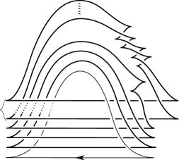
Figure 9: Non–loose Legendrian torus knot $T_{(2,2n+1)}$ in $S^{3}$ ($n\geq 1$).

The meaning of the picture is that we perform contact $(\pm 1)$–surgeries along the given Legendrian knots, the result being a contact 3–manifold containing the unframed knot $L(n)$ as a Legendrian knot. (For contact $(\pm 1)$–surgeries and surgery presentations see [3, 30].)

Lemma 6.1.

The contact structure $\xi_{n}$ defined by the surgery diagram of Figure 9 is the overtwisted contact structure on $S^{3}$ with Hopf invariant $d_{3}(\xi_{n})=1-2n$. The Legendrian knot $L(n)$ is smoothly isotopic to the torus knot $T_{2,2n+1}$ and is non–loose.

Proof.

Figure 10 gives a smooth surgery diagram corresponding to Figure 9.

2pt $-2$ at 28 52 $-1$ at 139 53 $-3$ [l] at 75 55 $-4$ [lt] at 51 80 $-4$ [rb] at 35 96 $0$ [r] at 203 53 $0$ [r] at 232 53 $L(n)$ [l] at 266 56 $(n)$ at 37 81

Figure 10: A smooth version of Figure 9.

The knot type of $L(n)$ and the underlying 3–manifold can be easily identified. The Kirby calculus moves of Figure 11 show that Figure 10 is equivalent to the left–hand side of Figure 12.

2pt $-1$ at 97 214 $-2$ at 20 213 $-4$ at 44 233 $-4$ at 22 252 $-3$ at 58 214 $0$ at 139 214 $0$ at 159 214 $(n)$ at 27 234 $L(n)$ at 190 239 $+1$ at 397 178 $L(n)$ at 434 225 $(n)$ at 263 236 $+1$ at 392 243 $+1$ at 379 229 $-1$ at 284 235 $-1$ at 261 255 $+1$ at 236 232 $+1$ at 234 216 $-2$ at 308 231 $-1$ at 367 27 $L(n)$ at 428 83 $+1$ at 235 85 $+1$ at 231 66 $(n)$ at 263 89 $-1$ at 288 91 $-1$ at 267 111 $-2$ at 371 88 $-2$ at 39 71 $-3$ at 82 68 $-2$ at 83 84 $-2$ at 81 150 $n-1$ at 152 114 $L(n)$ at 168 70 $-1$ at 97 14

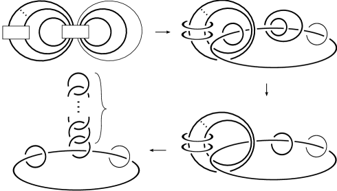
Figure 11: Kirby moves on Figure 10.

2pt $-1$ [b] at 76 6 $-2$ [rb] at 29 61 $-3$ [r] at 70 61 $-2$ [r] at 70 77 $-2$ [r] at 70 141 $n-1$ [l] at 125 107 $L(n)$ [b] at 139 61 $n$ at 285 55 $L(n)$ [b] at 286 102

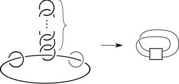
Figure 12: $L(n)$ is the torus knot $T_{2,2n+1}$.

Applying a number of “blow–downs” yields the right–hand side of Figure 12, veryfing that $L(n)$ is isotopic to the positive torus knot $T_{(2,2n+1)}$ in $S^{3}$.

Figures 9 and 10 can be used to determine the signature $\sigma(X)$ and the Euler characteristic $\chi(X)$ of the 4–manifold obtained by viewing the integral surgeries as 4–dimensional 2–handle attachments to $S^{3}\times[0,1]$. (As it is customary in Heegaard Floer theory, the 4-manifold $X$ denotes the cobordism between $S^{3}$ and the 3–manifold we get after performing the prescribed surgeries.) In addition, the rotation numbers define a second cohomology class $c\in H^{2}(X;{\mathbb{Z}})$, and a simple computation shows

$$\sigma(X)=-n-1,\ \ \chi(X)=n+3,\ \ c^{2}=-9n-1.$$

Since we apply two $(+1)$–surgeries, the formula

$$d_{3}(\xi)=\frac{1}{4}(c^{2}-3\sigma(X)-2\chi(X))+q$$

(with $q$ denoting the number of contact $(+1)$–surgeries) computes $d_{3}(\xi_{n})$ of the contact structure, providing $1-2n<0$ for all $n\in{\mathbb{N}}$. Since the unique tight contact structure $\xi_{st}$ on $S^{3}$ has vanishing Hopf invariant $d_{3}(\xi_{st})$, we get that $\xi_{n}$ is overtwisted. Applying contact $(-1)$–surgery along $L(n)$ we get a tight contact structure, since this $(-1)$–surgery cancels one of the $(+1)$–surgeries, and a single contact $(+1)$–surgery along the Legendrian unknot provides the Stein fillable contact structure on $S^{1}\times S^{2}$. Therefore there is no overtwisted disk in the complement of $L(n)$ (since such a disk would persist after the surgery), consequently $L(n)$ is non–loose. ∎

As it is explained in [25, Section 6], the Legendrian link underlying the surgery diagram for $\xi_{n}$ (together with the Legendrian knot $L(n)$) can be put on a page of an open book decomposition with planar pages, which is compatible with the standard contact structure $\xi_{st}$ on $S^{3}$. This can be seen by considering the annular open book decomposition containing the Legendrian unknot (and its Legendrian push–offs), and then applying the stabilization method described in [11] for the stabilized knots. The monodromy of this open book decomposition can be computed from the Dehn twists resulting from the stabilizations, together with the Dehn twists (right–handed for $(-1)$ and left–handed for $(+1)$) defined by the surgery curves. Notice that one of the left–handed Dehn twists is cancelled by the monodromy of the annular open book decomposition we started our procedure with. This procedure results in the monodromies given by the curves of Figure 13. We perform right–handed Dehn twists along solid curves and a left–handed Dehn twist along the dashed one.

2pt $L(n)$ [l] at 187 159 $(n)$ at 95 243

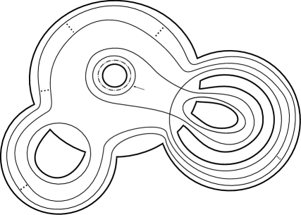
Figure 13: Monodromy of the open book decomposition compatible with $L(n)$. Solid curves represent right–handed Dehn twists, while the dashed one (parallel to $L(n)$) represents a left–handed Dehn twist.

The application of the lantern relation simplifies the monodromy factorization to the one shown in Figure 14.

2pt $L(n)$ at 149 137 $(n)$ [b] at 30 118

Figure 14: Simplified monodromy.

Notice that in the monodromy factorization given by Figure 13 there are Dehn twists along intersecting curves, hence these elements of the mapping class group do not commute. Therefore, strictly speaking, an order of the Dehn twists should be specified. Observe, however, that although the elements do not commute, the fact that there is only one such pair of intersecting curves implies that the two possible products are conjugate, and therefore give the same open book decomposition, allowing us to suppress the specification of the order.

Figure 15 helps to visualize the curves on ‘half’ of the Heegaard surface, and also indicates the chosen basis.

2pt $L(n)$ at 58 77 $a_{4}$ at 75 90 $a_{3}$ at 174 90 $a_{2}$ at 270 90 $a_{1}$ at 370 90 $(n)$ at 408 102

Figure 15: Another view of the monodromy. The diagram also indicates the chosen basis. (Notice that here $a_{4}$ intersects $L(n)$ in a unique point and not $a_{1}$.)

The open book decomposition found above equips $S^{3}$ with a Heegaard decomposition compatible with $L(n)$. The $\alpha$– and $\beta$–curves of this decomposition are given in Figure 16.

0pt $L(n)$ at 79 39 $\alpha_{4}$ at 227 58 $\alpha_{3}$ at 218 193 $\alpha_{2}$ at 222 236 $\alpha_{1}$ at 223 372 $\beta_{1}$ at 109 406 $\beta_{2}$ at 90 299 $\beta_{3}$ at 93 202 $\beta_{4}$ at 88 100 $n$ at 161 434 $w$ at 128 18 $z$ at 50 211 $L$ at 141 116 $M$ at 155 98 $B_{3}$ at 205 211 $X_{1}$ at 137 200 $C_{2}$ at 157 199 $X_{2}$ at 194 199 $Y_{2}$ at 167 218 $B_{4}$ at 149 218 $Y_{1}$ at 121 217 $B_{1}$ at 86 257 $P$ at 166 303 $B_{2}$ at 218 277 $Q$ at 124 311 $A_{1}$ at 88 381 $A_{2}$ at 133 392 $A_{n}$ at 176 405 $A_{n+1}$ [l] at 218 329 $C_{1}$ at 87 167 $D=D_{1}$ [r] at 91 68

Figure 16: The Heegaard decomposition compatible with $L(n)$.

Recall that we get the $b_{i}$ arcs by the usual perturbation of the $a_{i}$’s and the action of the monodromy yields a Heegaard decomposition for $S^{3}$ with the distinguished point ${\bf{x}}$ in ${\mathbb{T}}_{\alpha}\cap{\mathbb{T}}_{\beta}$ determining the Legendrian invariant $\widehat{\mathfrak{L}}(L(n))$. A warning about orientations is in place. We illustrated the monodromy curves on the page $S_{+1}$ containing the Legendrian knot $L(n)$, but their action must be taken into account on the page $S_{-1}$, which comes in the Heegaard surface with its opposite orientation; hence right–handed Dehn twists take curves to the left on the Heegaard surface and vice versa. The basepoint $z$ is placed in the ‘large’ region of the page $S_{+1}$, while the point $w$ is in the strip between $a_{1}$ and $b_{1}$ shown in Figure 16. This choice determines the orientation on $L(n)$.

Recall that since $L(n)$ is isotopic to the positive torus knot $T_{(2,2n+1)}$, the Legendrian invariant is given by an element of $\widehat{\mathrm{HFK}}(-S^{3},T_{(2,2n+1)})$, which is isomorphic to $\widehat{\mathrm{HFK}}(S^{3},T_{(2,-(2n+1))})$. This latter group is determined readily from the Alexander polynomial and the signature of the knot (since it is alternating), cf. [36, 39]. In fact, we have

$$\widehat{\mathrm{HFK}}_{n+s}(S^{3},T_{(2,-(2n+1))},s)\cong\left\{\begin{array}[]{ll}\mathbb{F}&{\text{if $|s|\leq n$}}\\ 0&{\text{otherwise.}}\end{array}\right.$$ (6.1)

After these preparations we are ready to determine the invariants of the Legendrian knots discussed above.

Proposition 6.2.

The homology class $\widehat{\mathfrak{L}}(L(n))$ is determined by the unique nontrivial homology class in Alexander grading $1-n$ in $\widehat{\mathrm{HFK}}(S^{3},T_{(2,-2n-1)})$.

Proof.

We claim that in the Heegaard diagram of Figure 16 the point $A_{1}B_{1}C_{1}D_{1}$ (representing the Legendrian invariant $\widehat{\mathfrak{L}}(L(n))$) is the only intersection point in Alexander grading $1-n$.

We sketch the argument establishing this. We can orient every $\alpha$– and $\beta$–curve in the diagram so that their intersection matrix (whose $(i,j)^{th}$ entry is the algebraic intersection of $\alpha_{i}$ with $\beta_{j}$) is

$$M=\left(\begin{array}[]{rrrr}n+1&-1&0&0\\ -1&4&-2&0\\ 0&-2&2&-1\\ 0&0&-1&1\end{array}\right).$$

Note that for this particular diagram, the absolute values of the algebraic intersection number and the geometric intersection numbers coincide.

A simple calculation shows that there are $16n+19$ intersecton points in ${\mathbb{T}}_{\alpha}\cap{\mathbb{T}}_{\beta}$. To calculate the relative Alexander gradings of intersection points, it is convenient to organize them into types: specifically, the intersection points of $\mathbb{T}_{\alpha}$ and $\mathbb{T}_{\beta}$ correspond to permutations $\sigma$ and then $4$-tuples in $\prod\alpha_{i}\cap\beta_{\sigma(i)}$, which in terms of the notation of Figure 16 are given by quadruples of letters; specifically, intersection points all have one of the following five types

$$\begin{array}[]{lllll}ABCD&PQCD&AXYD&ABLM&PQLM.\end{array}$$

We begin by calculating relative Alexander gradings of intersection points of the same type. Consider first the relative gradings between points of the form $A_{i}\mbox{$\star\star\star$}$ and $A_{i+1}\mbox{$\star\star\star$}$, where now $\star\star\star$ is a fixed triple of intersection points. Start from an initial path $\delta$ which travels from $A_{i}$ to $A_{i+1}$ along $\alpha_{1}$, then back from $A_{i+1}$ to $A_{i}$ along $\beta_{1}$. We add to this cycle copies of $\alpha_{i}$ and $\beta_{j}$ to obtain a null-homologous cycle. This can be done since the $\alpha_{i}$’s and $\beta_{j}$’s span $H_{1}(\Sigma)$, which follows from the fact that the ambient 3–manifold is $S^{3}$. Concretely, we need to solve the expression

$$\sum n_{i}[\alpha_{i}]+\sum m_{j}[\beta_{j}]+[\delta]=0$$

for $n_{i}$ and $m_{j}$. In fact, all we are concerned about is the difference in local multiplicities at $z$ and $w$ in the null-homology of the above expression. Since $z$ and $w$ are separated by $\alpha_{4}$, and our initial curve $\delta$ is supported on $\alpha_{1}$ and $\beta_{1}$, this difference is given by the multiplicity $n_{4}$ of $\alpha_{4}$ in the above expression. In view of the fact that $\#\beta_{i}\cap\beta_{j}=0$, $n_{4}$ can be obtained as the last coefficient of $M^{-1}v$, where $v$ is the vector whose $i^{th}$ coordinate is $\#\delta\cap\beta_{j}$ and $M$ is the incidence matrix. We can find paths of the above type $\delta$ connecting $A_{i}$ and $A_{i+1}$ whose intersection numbers with the $\beta_{j}$’s are given by the vector $(1,0,0,0)$, hence giving that the Alexander grading of $A_{i}\mbox{$\star\star\star$}$ is two smaller than the Alexander grading of $A_{i+1}\mbox{$\star\star\star$}$. We express this by saying that the relative gradings of the $A_{i}$ are given by $2i$. Repeating this procedure for the other curves, we find that relative gradings of $B_{1},...,B_{4}$ (completed by a fixed triple to quadruples of intersection points) are given by $0$, $2n$, $4n+2$, and $2n+1$ respectively; for $C_{1}$ and $C_{2}$ the relative gradings are $0$ and $2n+1$ respectively, for $X_{1}$ and $X_{2}$ they are $0$ and $2n+1$, and they are also $0$ and $2n+1$ for $Y_{1}$ and $Y_{2}$. Putting these together, we can calculate the relative Alexander gradings of any two intersection points of the same type.

To calculate the relative Alexander gradings of points of different types, we use three rectangles. Specifically, intersection points of the form $PQ\mbox{$\star\star$}$ and $A_{n+1}B_{1}\mbox{$\star\star$}$ (where here $\star\star$ denotes some fixed pair of intersection points) have equal Alexander gradings, shown by the rectangle with vertices $PB_{1}QA_{n+1}$, avoiding both $w$ and $z$. Similar argument relates points of type $X_{1}Y_{1}\mbox{$\star\star$}$ to the ones of type $B_{4}C_{1}\mbox{$\star\star$}$. The rectangle $LDMC_{1}$ contains $w$ once, showing that the Alexander gradings of elements of the form $LM\mbox{$\star\star$}$ are one less than the Alexander gradings of elements of the form $C_{1}D\mbox{$\star\star$}$. This allows us to calculate the relative Alexander gradings of any two intersection points.

Given this information, it is now straightforward to see that there are no other intersection points in the same Alexander grading as $A_{1}B_{1}C_{1}D_{1}$, and hence that it represents a homologically nontrivial cycle in $\widehat{\mathrm{HFK}}(S^{3},T_{(2,-(2n+1))})$. Thus, we have shown that for all $n\in{\mathbb{N}}$, the class $\widehat{\mathfrak{L}}(L(n))$ is a nontrivial generator in $\widehat{\mathrm{HFK}}(S^{3},T_{(2,-(2n+1))})$.

In fact, the absolute Alexander grading of generators is pinned down by the following symmetry property: the Alexander grading is normalized so that the parity of the number of points of Alexander grading $i$ coincides with the parity of the number of points of Alexander grading $-i$. Using this property, one finds that $A_{1}B_{1}C_{1}D_{1}$ is supported in Alexander grading $1-n$. ∎

Remark 6.3.

Recall (cf. [36, 39]) that

$$\mathrm{HFK}^{-}(S^{3},T_{(2,-(2n+1))})\cong\mathbb{F}^{n}\oplus\mathbb{F}[U],$$ (6.2)

where the top generator of the free $\mathbb{F}[U]$–module is at $(A=n,M=2n)$ while the $n$ generators of the $\mathbb{F}^{n}$ summand are of bi–degrees

$$(A=n-1-2i,\quad M=2n-1-2i),\quad i=0,\ldots,n-1.$$

It is not hard to show that the above computation implies that ${\mathfrak{L}}(L(n))$ is determined by the unique nonzero $U$–torsion element of $\mathrm{HFK}^{-}(S^{3},T_{(2,-(2n+1))})$ in Alexander grading $1-n$.

Negative Legendrian torus knots $T_{(2,-(2n-1))}$ in overtwisted contact $S^{3}$’s

For $k,l\geq 0$ let us consider the knot $L_{k,l}$ in the contact 3–manifold $(Y_{k,l},\xi_{k,l})$ given by the surgery presentation of Figure 17. Let $n=k+l+2$.

2pt $L_{k,l}$ [l] at 453 55 $+1$ [l] at 458 82 $+1$ [l] at 454 107 $-1$ [l] at 453 131 $-1$ [l] at 514 154 $-1$ [l] at 513 201 $l$ at 469 391 $k$ at 46 343

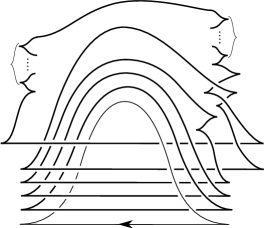
Figure 17: Non–loose Legendrian $T_{(2,-(2n-1))}$ torus knot in $S^{3}$.

Proposition 6.4.

The contact 3–manifold specified by the surgery diagram of Figure 17 is $(S^{3},\xi_{k,l})$ with $d_{3}(\xi_{k,l})=2l+2$, hence $\xi_{k,l}$ is overtwisted. The Legendrian knot $L_{k,l}$ as a smooth knot is isotopic to the negative $(2,2n-1)$ torus knot $T_{(2,-(2n-1))}$, and it is non–loose in $(S^{3},\xi_{k,l})$.

Proof.

The simple Kirby calculus argument illustrated in Figure 18

2pt $L_{k,l}$ at 187 255 $-1$ at 106 227 $0$ at 142 226 $0$ at 161 226 $-3$ at 15 200 $-3$ at 38 209 $-n$ at 29 232

$-n$ at 230 258 $-2$ at 265 253 $L_{k,l}$ at 399 249 $-2$ at 295 214 $1$ at 323 196 $1$ at 361 258 $1$ at 343 253

$-n$ at 38 158 $-2$ at 86 167 $-1$ at 115 107 $L_{k,l}$ at 194 157 $-2$ at 133 168

$-n$ at 257 150 $-1$ at 294 108 $1$ at 328 125 $L_{k,l}$ at 381 147 $-1$ at 375 110

$-n$ at 84 68 $0$ at 63 25 $L_{k,l}$ at 182 68 $T_{2,-(2n-1)}\subset S^{3}$ (after two slides) [l] at 233 39

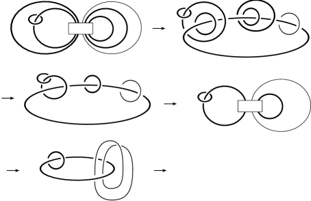
Figure 18: Kirby moves on the diagrams of Figure 17.

shows that the 3–manifold $Y_{k,l}$ is $S^{3}$, while the formula

$$d_{3}(\xi_{k,l})=\frac{1}{4}(c^{2}-3\sigma-2b_{2})+q$$

of [4] computes the Hopf invariant of $\xi_{k,l}$. As always, $\sigma$ and $b_{2}$ denote the signature and the second Betti number of the 4–manifold $X$ specified by the underlying smooth surgery diagram, while $c\in H^{2}(X;{\mathbb{Z}})$ is specified by the rotation numbers of the contact surgery curves, and $q$ is the number of $(+1)$–surgeries. Simple algebra verifies that

$$d_{3}(\xi_{k,l})=2l+2\geq 2,$$

and since the unique tight structure on $S^{3}$ has vanishing Hopf invariant, we get that $\xi_{k,l}$ is overtwisted. Following the Kirby moves of Figure 18 with the knot $L_{k,l}$ we arrive to the last surgery picture of Figure 18, and by sliding $L_{k,l}$ twice over the $(-n)$–framed unknot and cancelling the pair we see that $L_{k,l}$ is, in fact, isotopic to the negative $(2,2n-1)$ torus knot $T_{(2,-(2n-1))}\subset S^{3}$.

If contact $(-1)$–surgery on $L_{k,l}$ provides a tight contact structure, then $L_{k,l}$ is obviously non–loose, since any overtwisted disk in its complement would give an overtwisted disk in the surgered manifold. In our case, however, contact $(-1)$–surgery simply cancels one of the $(+1)$–surgeries defining $\xi_{k,l}$, and since a single contact $(+1)$–surgery on the Legendrian unknot provides the contact boundary of the Stein 1–handle (cf. [23]), we get that $(-1)$–surgery along $L$ provides a Stein fillable contact structure. ∎

Remark 6.5.

In fact, by stabilizing $L_{k,l}$ on the left and then performing a contact $(-1)$–surgery we still get a tight contact 3–manifold: it will be Stein fillable if we perform only one stabilization, and not Stein fillable but tight for more stabilizations. The tightness of the result of these latter surgeries were verified in [17] by computing the contact Ozsváth–Szabó invariants of the resulting contact structures. Notice that this observation implies that after arbitrary many left stabilizations $L_{k,l}$ remains non–loose, which, in view of Proposition 5.2, is a necessary condition for ${\mathfrak{L}}(L_{k,l})$ to be nonvanishing. (Finally note that performing contact $(-1)$–surgery on $L_{k,l}$ after a single right stabilization provides an overtwisted contact structure (cf. now [17, Section 5])). In contrast, for the non–loose knots $L(n)$ of the previous subsection (also having nontrivial ${\mathfrak{L}}$–invariants) the same intuitive argument does not work, since some negative surgery on the knot $L(n)$ will produce a contact structure on the 3–manifold $S^{3}_{2n-1}(T_{2,2n+1})$ and since this 3–manifold does not admit any tight contact structure [24], the result of the surgery will be overtwisted independently on the chosen stabilizations. Nevertheless, the overtwisted disk in the 3–manifold obtained by only negative stabilizations cannot be in the complement of the knot $L(n)$, since such stabilizations are still non–loose (shown by the nonvanishing of the invariant $\widehat{{\mathfrak{L}}}(L(n))$).

Next we want to determine the classical invariants of $L_{k,l}$. Considering the problem slightly more generally, and let $L\subset Y$ be a null–homologous Legendrian knot in a contact 3–manifold $(Y,\xi)$. Assume furthermore that $Y$ is a rational homology 3–sphere. The knot $L$ has two “classical invariants”: the Thurston–Bennequin and the rotation numbers $\operatorname{tb}(L),\operatorname{rot}(L)$. Recall that the Thurston–Bennequin invariant of a Legendrian knot is defined as the framing induced by the contact 2–plane field distribution on the knot, hence, given an orientation for the knot, it naturally gives rise to a homology class $\operatorname{TB}\in H_{1}(Y-L;\mathbb{Z})$ (supported in a tubular neighborhood of $L$). Fixing a Seifert surface $F$ for $L$, the oriented intersection number of $\operatorname{TB}$ with $F$ provides a numerical invariant, called the Thurston–Bennequin number $\operatorname{tb}(L)\in\mathbb{Z}$. This intersection number is independent of the choice of the Seifert surface; moreover, the Thurston–Bennequin number is independent of the orientation of $L$ since the orientation of $\operatorname{TB}$ and the orientation of $F$ both depend on this choice. Analogously, the rotation $\operatorname{rot}$ of $L$ is the relative Euler class of $\xi$ when restricted to $Y-L$, with the trivialization given by the tangents of $L$. Again, a Seifert surface for $L$ can be used to turn this class uniquely into an integer, also denoted by $\operatorname{rot}(L)$. Note that unlike the Thurston–Bennequin number, the sign of the rotation number does depend on the orientation of $L$.

Suppose that ${\mathbb{S}}={\mathbb{S}}_{+}\cup{\mathbb{S}}_{-}\subset(S^{3},\xi_{st})$ is a contact $(\pm 1)$–surgery presentation of the contact 3–manifold $(Y,\xi)$ and $L$ is a Legendrian knot in $(S^{3},\xi_{st})$ disjoint from ${\mathbb{S}}$, null–homologous in $Y$. The Thurston–Bennequin and rotation numbers of $L$ in $(Y,\xi)$ can be obtained from the Thurston–Bennequin and rotation numbers of the individual components of ${\mathbb{S}}$ and $L$ through the following data. Let $\operatorname{tb}_{0}$ denote the Thurston–Bennequin number of $L$ as a knot in the standard contact 3–sphere (which, in terms of a front projection, is equal to the writhe minus half the number of cusps). Writing ${\mathbb{S}}=\cup_{i=1}^{n}L_{i}$, let $a_{i}$ be the integral surgery coefficient on the link component $L_{i}$; i.e. $a_{i}=\operatorname{tb}(L_{i})\pm 1$ if $L_{i}\in{\mathbb{S}}_{\pm}$. Define the linking matrix

$$M(a_{0},a_{1},...,a_{n})=\left(m_{i,j}\right)_{i,j=0}^{n}$$

where

$$m_{i,j}:=\left\{\begin{array}[]{ll}a_{i}&{\text{if $i=j$}}\\ {\mathrm{lk}}(L_{i},L_{j})&{\text{if $i\neq j$,}}\end{array}\right.$$

with the convention that $L=L_{0}$ and ${\mathbb{S}}=\cup_{i=1}^{n}L_{i}$. Similarly, let $M(a_{1},...,a_{n})$ denote the matrix $\left(m_{i,j}\right)_{i,j=1}^{n}$. Consider the integral rotation numbers $r_{0},...,r_{n}$ obtained from our Legendrian knot $L$ and Legendrian presentation as a link in $S^{3}$.

Lemma 6.6.

Suppose that ${\mathbb{S}}={\mathbb{S}}_{+}\cup{\mathbb{S}}_{-}\subset(S^{3},\xi_{st})$ is a contact $(\pm 1)$–surgery presentation of the contact 3–manifold $(Y,\xi)$ and $L$ is a Legendrian knot in $(S^{3},\xi_{st})$ disjoint from ${\mathbb{S}}$, null–homologous in $Y$. Then the Thurston-Bennequin and rotation numbers $\operatorname{tb}(L)$ and $\operatorname{rot}(L)$ can be extracted from the above data by the formulae:

$$\operatorname{tb}(L)=\operatorname{tb}_{0}+\frac{\det(M(0,a_{1},...,a_{n}))}{\det(M(a_{1},...,a_{n}))}$$ (6.3)

and

$$\operatorname{rot}(L)=r_{0}-\langle\left(\begin{array}[]{c}r_{1}\\ \vdots\\ r_{n}\end{array}\right),M^{-1}\cdot\left(\begin{array}[]{c}\operatorname{lk}(L_{0},L_{1})\\ \vdots\\ \operatorname{lk}(L_{0},L_{n}),\end{array}\right)\rangle,$$ (6.4)

where $M=M(a_{1},...,a_{n})$.

Proof.

We turn to the verification of Equation (6.4), after a few preliminary observations. Let $\mu_{i}\subset S^{3}-(L\cup{\mathbb{S}})$ be a meridian for $L_{i}\subset L\cup{\mathbb{S}}$, and $\lambda_{i}$ be its corresponding longitude. Recall that $H_{1}(S^{3}-(L\cup{\mathbb{S}}))$ is a free $\mathbb{Z}$-module, generated by the meridians $\mu_{i}$ (we continue with the convention that the $i=0$ component of the link $L\cup{\mathbb{S}}$ is $L$). We can express the homology class of $\lambda_{i}$ in terms of the other meridians by the expression

$$\lambda_{i}=\sum_{j\neq i}\operatorname{lk}(L_{i},L_{j})\cdot\mu_{j}.$$

The homology groups of the surgered manifold are gotten from the homology groups of the link complement by dividing out by the relations $a_{i}\mu_{i}+\lambda_{i}=0$ for $i=1,...,n$; more precisely, $H_{1}(S^{3}-(L\cup{\mathbb{S}}))$ is freely generated by $\mu_{0},...,\mu_{n}$, while $H_{1}(Y-L)\cong\mathbb{Z}$ is obtained from this free group by dividing out the $n$ relations

$$a_{i}\cdot\mu_{i}+\sum_{j\neq i}\operatorname{lk}(L_{i},L_{j})\cdot\mu_{j}=0,\quad i=1,\ldots,n.$$

The rotation numbers $r_{i}$ can be thought of as follows. Let $e(\xi,L\cup{\mathbb{S}})\in H^{2}(S^{3},L\cup{\mathbb{S}})$ denote the relative Euler class of $\xi$ relative to the trivialization it inherits along $L\cup{\mathbb{S}}$. Then, the rotation numbers are the coefficients in the expansion of the Poincaré dual $\operatorname{PD}[e(\xi,L\cup{\mathbb{S}})]\in H_{1}(S^{3}-(L\cup{\mathbb{S}}))$ in terms of the basis of meridians $\operatorname{PD}[e(\xi,L\cup{\mathbb{S}})]=\sum_{i=0}^{n}r_{i}\cdot\mu_{i}$. Similarly, $H_{1}(Y-L)\cong\mathbb{Z}$ is generated by $\mu_{0}$, the meridian of $L$, and the rotation number $\operatorname{rot}(L)$ is calculated by $\operatorname{PD}(e(\xi,L))=\operatorname{rot}(L)\cdot\mu_{0}$. Note also that $\operatorname{PD}[e(\xi,L)]$ is the image of $\operatorname{PD}[e(\xi,L\cup{\mathbb{S}})]$ under the inclusion $j\colon S^{3}-(L\cup{\mathbb{S}})\subset Y-L$. Thus, to find $\operatorname{rot}(L)$, it suffices to express $j_{*}(\mu_{i})$ in terms of $\mu_{0}$. Write

$$\Lambda=\left(\begin{array}[]{c}\operatorname{lk}(L_{0},L_{1})\\ \vdots\\ \operatorname{lk}(L_{0},L_{n}),\end{array}\right) R=\left(\begin{array}[]{c}r_{1}\\ \vdots\\ r_{n}\end{array}\right).$$ and

In view of our presentation for $H_{1}(S^{3}-L)$, we see that for all $i>0$ we have $\mu_{i}=c_{i}\cdot\mu_{0}$, where $c_{i}$ is the $i^{th}$ entry in the vector $-M^{-1}\cdot\Lambda$. It follows that

$$\sum_{i=0}^{n}r_{i}\cdot\mu_{i}=(r_{0}-\langle R,M^{-1}\cdot\Lambda\rangle)\cdot\mu_{0},$$

estabilishing Equation (6.4).

We turn now to Equation (6.3). Choose $a_{0}$ so that the curve $\lambda^{\prime}=a_{0}\cdot\mu_{0}+\lambda_{0}$ is null–homologous in $Y-L$. Letting $\operatorname{TB}$ denote the Thurston–Bennequin framing curve of $L=L_{0}$, we have that

$$\operatorname{TB}=\operatorname{tb}_{0}\cdot\mu_{0}+\lambda_{0}=\operatorname{tb}(L)\cdot\mu_{0}+\lambda^{\prime};$$

thus $\operatorname{tb}(L)-\operatorname{tb}_{0}=-a_{0}$. In view of our presentation for this first homology group, we see that $a_{0}$ is determined by the condition that

$$0 = \left|\begin{array}[]{llll}a_{0}&\operatorname{lk}(L_{0},L_{1})&...&\operatorname{lk}(L_{0},L_{n})\\ \operatorname{lk}(L_{0},L_{1})&a_{1}&...&\operatorname{lk}(L_{0},L_{1})\\ \vdots&\vdots&\ddots&\vdots\\ \operatorname{lk}(L_{n},L_{0})&\operatorname{lk}(L_{n},L1)&\ldots&a_{n}\end{array}\right|$$

$$= a_{0}\cdot\det(M(a_{1},...,a_{n}))+\det(M(0,a_{1},...,a_{n})).$$

Equation (6.3) follows. ∎

Lemma 6.7.

With the orientation given by Figure 17, the Thurston–Bennequin and rotation numbers of the knot $L_{k,l}$ are given by

$$\operatorname{tb}(L_{k,l})=-4(k+l)-6\quad{\mbox{and}}\quad\operatorname{rot}(L_{k,l})=-6l-2k-7.$$

Proof.

Applying Formulae (6.3) and (6.4) to the surgery diagrams defining $L_{k,l}$, simple algebra gives the statement of the lemma. ∎

As it is explained in the previous subsection (resting on observations from [25, Section 6]), the surgery diagram for $\xi_{k,l}$ (together with the Legendrian knot $L_{k,l}$) can be put on a page of an open book decomposition with planar pages, which is compatible with the standard contact structure $\xi_{st}$ on $S^{3}$. The diagram for all choices of $k$ and $l$ is less apparent, hence we restrict our attention first to $k=0$. In this case we get the monodromies defined by the curves of Figure 19.

2pt $L_{0,l}$ at 195 158 $l$ at 97 104

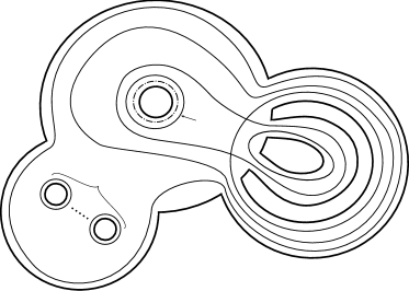
Figure 19: Monodromy of the open book decomposition compatible with $L_{0,l}$.

The application of the lantern relation simplifies the monodromy factorization to the one illustrated in Figure 20.

2pt $L_{0,l}$ at 155 140 $l$ at 389 155

Figure 20: The simplified monodromy of the open book for $L_{0,l}$.

Figure 21 helps in visualizing the curves on ‘half’ of the Heegaard surface. The diagram also indicates the chosen basis.

2pt $L_{0,l}$ at 47 70 $l+1$ at 349 154

Figure 21: Another view of the open book for $L_{0,l}$.

Notice that in the monodromy illustrated in Figure 19 there are Dehn twists with intersecting curves, hence these elements of the mapping class group do not commute. As before, the two products are conjugate, hence there is no need to record the order.

In a similar spirit the general diagrams could be deduced — since we will not use them in our computations, we will be content with working on a further special case when $k=1$ and $l\geq 1$; the result is given by Figure 22.

2pt $L(1,l)$ [lb] at 110 152 $l-1$ at 378 136

Figure 22: The monodromy factorization for $L(1,l)$ with $l\geq 1$.

We just note here that in these cases we need to apply the lantern relation twice to get commuting Dehn twists as illustrated in Figure 22. For this reason, these monodromy factorizations contain two left–handed Dehn twists. In Figure 23 the monodromy for $L(1,l)$ with $l\geq 1$ is represented on ’half’ of the Heegaard surface.

2pt $L(1,l)$ at 39 74 $l-1$ at 185 151

Figure 23: The open book for $L(1,l)$ with $l\geq 1$.

The open book decomposition found above equips $S^{3}$ with a Heegaard decomposition compatible with $L_{k,l}$; the $\alpha$– and $\beta$–curves of this decomposition for $k=0$ are given by Figure 24 when $l=0$ and by Figure 25 when $l>0$.

2pt $L_{0,0}$ at 76 41 $w$ at 130 18 $z$ at 44 161

Figure 24: The Heegaard decomposition for $L(0,0)$.

2pt $z$ at 45 306 $w$ at 145 18 $L_{0,l}$ at 81 43 $A$ at 78 661 $B$ at 153 710 $C$ at 153 622 $C^{\prime}$ at 206 622

Figure 25: The Heegaard decomposition for $L(0,l)$, $l>0$.

Recall that we get the $b_{i}$ curves by the usual perturbation of the $a_{i}$’s and the action of the monodromy yields a Heegaard decomposition for $S^{3}$ with the distinguished point ${\bf{x}}$ in ${\mathbb{T}}_{\alpha}\cap{\mathbb{T}}_{\beta}$ determining the Legendrian invariant. As usual, the basepoint $z$ is placed in the ‘large’ region of the page $S_{+1}$, while the point $w$ giving rise to $\widehat{\mathfrak{L}}$ is in the strip between $a_{1}$ and $b_{1}$, as indicated in the pictures. It is easy to see that moving $w$ to the other domain in the strip gives $\widehat{\mathfrak{L}}=0$, because there is a holomorphic disk running into ${\bf{x}}$.

Recall that $L_{k,l}$ is isotopic to the negative torus knot $T_{(2,-(2n-1))}$. The group $\widehat{\mathrm{HFK}}(-S^{3},T_{(2,-(2n-1))})$ is isomorphic to the Floer homology $\widehat{\mathrm{HFK}}(S^{3},T_{(2,2n-1)})$ of the positive torus knot $T_{(2,2n-1)}$. In this case we have the following (compare Equation (6.1)):

$$\widehat{\mathrm{HFK}}_{s-n+1}(S^{3},T_{(2,2n-1)},s)\cong\left\{\begin{array}[]{ll}\mathbb{F}&{\text{if $|s|\leq n-1$}}\\ 0&{\text{otherwise.}}\end{array}\right.$$ (6.7)

After these preparations we are ready to determine the invariants of some of the Legendrian knots discussed above. The computation admits a relatively simple scheme when $k=0$, so we start with that case.

Theorem 6.8.

Let $L_{0,l}$ be given the orientation specified by the diagram of Figure 24 or Figure 25. Then, $\widehat{\mathfrak{L}}(L_{0,l})\neq 0$.

Proof.

We show that the intersection point ${\bf{x}}_{0}\in\widehat{\mathrm{CFK}}$, which determines $\widehat{\mathfrak{L}}(L_{0,l})$, is alone in its Alexander grading.

Claim: Any other intersection point ${\bf{y}}$ in the Heegaard decomposition given by Figure 24 or 25 has Alexander grading $A({\bf{y}})$ strictly less than $A({\bf{x}}_{0})$.

The claim, in turn, will be proved by induction on $l$. For $l=0$ (which means that we are computing Legendrian invariants of a Legendrian left–handed trefoil knot in an overtwisted $S^{3}$) the explicit determination of the Alexander gradings of each of the 19 intersection points verifies the statement. To do this we only need to find domains connecting any two intersection points, and their relative Alexander grading is the multiplicity of the domain containing the basepoint $w$. A straightforward linear algebra argument similar to the one outlined in the proof of Proposition 6.2 shows that all top three degress contain unique intersection points (giving rise to homology elements), while the remaining 16 intersection points are of strictly smaller Alexander grading.

The argument for the inductive step proceeds as follows: Notice that by deleting the top–most $\alpha$– and $\beta$–curves (containing the point $A$ of Figure 25) in the Heegaard decomposition ${\mathfrak{H}}_{1}$ (and destabilizing the Heegaard surface) we get a Heegaard decomposition ${\mathfrak{H}}_{0}$ adapted to $T_{(2,2n-3)}$. Repeating this procedure one more time we get a Heegaard decomposition ${\mathfrak{H}}_{-1}$, which will be a decomposition adapted to $T_{(2,2n-5)}$.

Note that the intersection matrix of the $\alpha$– and $\beta$–curves has the following form

$$\left(\begin{array}[]{rrrrrrrr}-2&1&0&0&0&0&0\\ 1&-2&1&0&0&0&0\\ 0&1&\ddots&\ddots&0&0&0\\ 0&0&\ddots&-2&1&0&0\\ 0&0&0&1&-4&2&0\\ 0&0&0&0&2&-2&1\\ 0&0&0&0&0&1&-1\end{array}\right)$$

Now let us group the intersection points of the original diagram into types $A,B$ and $C$ depending on their coordinate on the top–most $\beta$–curve. It is easy to see that points in each $A$ and $B$ are in 1-1 correspondence with intersections in ${\mathfrak{H}}_{0}$, while points in $C$ are in 1-1 correspondence with points in ${\mathfrak{H}}_{-1}$. From the form of this matrix it is easy to see that the relative gradings within the groups coincide with the relative gradings in their respective Heegaard diagrams ${\mathfrak{H}}_{0}$ and ${\mathfrak{H}}_{-1}$. As usual, let ${\bf{x}}_{0}$ denote the intersection point representing the Legendrian invariant, $B_{{\bf{x}}_{0}}$ the point with the same coordinates except on the top-most $\alpha$–circle, where $A$ is substituted with $B$. Finally, $C_{{\bf{x}}_{0}}$ will denote the intersection point where on the top–most $\beta$–circle we choose $C$ (and so on the top–most $\alpha$–circle we should take $C^{\prime}$) and otherwise we take the same intersection points as in ${\bf{x}}_{0}$. Our inductive assumption is that ${\bf{x}}_{0}$, $B_{{\bf{x}}_{0}}$ and $C_{{\bf{x}}_{0}}$ are of highest Alexander gradings in the groups $A,B,C$, respectively. Therefore to conclude the argument we only need to compare the gradings of these intersection points. This relative computation can be performed locally near the top–most $\alpha$– and $\beta$–curves and we get that $A({\bf{x}})-A(B_{{\bf{x}}})=2$ and $A({\bf{x}})-A(C_{{\bf{x}}})=2$. By the inductive hypothesis this shows that ${\bf{x}}_{0}$ is the unique cycle in the top Alexander grading, concluding the proof. ∎

Note that the relation found in the proof of Theorem 6.8 amongst the Alexander gradings of the intersection points of the diagrams ${\mathfrak{H}}_{i}$ ($i=\pm 1,0$) is a manifestation of the fact that the symmetrized Alexander polynomial $\Delta_{n}(t):=\Delta_{T_{(2,2n-1)}}(t)$ satisfies the identity

$$\Delta_{n}(t)=(t-t^{-1})\Delta_{n-1}(t)-\Delta_{n-2}(t).$$

We consider two more cases, which can be handled by explicit methods: $L_{1,1}$ and $L_{1,2}$. In these cases the Alexander grading alone is not sufficient to calculate the homology class; we need a little analysis of holomorphic disks. We begin with the first of these:

Theorem 6.9.

Let $L_{1,1}$ be given the orientation specified by the diagram of Figure 26. Then, $\widehat{\mathfrak{L}}(L_{1,1})\neq 0$.

Recall that $L_{1,1}$ represents the negative torus knot $T_{(2,-7)}$.

Proof.

Consider the adapted Heegaard diagram for $L_{1,1}$ exhibited in Figure 26.

2pt $w$ at 141 18 $z$ at 31 258 $L_{1,1}$ at 77 41 $E$ at 82 68 $R$ at 157 99 $S$ at 139 117 $D_{1}$ at 82 165 $V_{1}$ at 142 199 $D_{2}$ at 172 200 $V_{2}$ at 192 198 $C_{1}$ at 78 257 $C_{2}$ at 148 218 $M_{1}$ at 99 210 $M_{2}$ at 166 218 $C_{3}$ at 184 217 $C_{4}$ at 220 261 $C_{5}$ at 218 273 $C_{6}$ at 215 289 $P_{2}$ at 176 304 $C_{7}$ at 159 293 $P_{1}$ at 136 293 $B_{3}$ at 156 314 $B_{2}$ at 134 313 $Q_{1}$ at 113 312 $X$ at 169 399 $Y$ at 131 409 $B_{1}$ at 85 392 $A_{1}$ at 76 449 $A_{2}$ at 148 497

Figure 26: Adapted Heegaard diagram for $L_{1,1}$.

Analyzing this diagram as in the other cases, we see that there are $149$ elements in $\mathbb{T}_{\alpha}\cap\mathbb{T}_{\beta}$, seven of which with the same Alexander grading as the point ${\bf{x}}_{0}$ determining $\widehat{\mathfrak{L}}(L(1,1))$. Indeed, in the notation suggested by that diagram, the seven intersection points in Alexander grading $A=1$ are

$$\begin{array}[]{llll}A_{2}B_{2}C_{7}D_{1}E,&A_{2}D_{1}EP_{2}Q_{1},&A_{2}D_{1}EP_{1}Q_{1},&A_{2}B_{1}C_{6}D_{1}E,\\ XYC_{6}D_{1}E,&A_{1}B_{2}C_{5}D_{1}E,&A_{1}B_{1}C_{1}D_{1}E={\bf{x}}_{0}.&\end{array}$$

Since ${\bf{x}}_{0}$ is a cycle, it can be thought of as determining a subcomplex of $\widehat{\mathrm{CFK}}(L_{1,1},1)$. The quotient complex then is generated by the six remaining generators in the given Alexander gradings. Indeed, it is straightforward to find the positive homotopy classes connecting these six generators with Maslov index one. There are six, and five of these are rectangles, and hence admit holomorphic representatives. The sixth (connecting $XYC_{6}D_{1}E$ to $A_{1}B_{2}C_{5}D_{1}E$) is also a planar surface, and it is not difficult to verify directly that it, too, always has a holomorphic representative. We assemble this information of the chain complex in Figure 27.

Figure 27: Part of the chain complex for $L_{1,1}$. This is the quotient of $\widehat{\mathrm{CFK}}(L_{1,1},1)$ by the generator $A_{1}B_{1}C_{1}D_{1}E$. Arrows indicate differentials.

It is straightforward to verify that this complex is acyclic. It follows at once that ${\bf{x}}_{0}$ represents the nontrivial homology class in $\widehat{\mathrm{HFK}}(L_{1,1},1)$. ∎

In a similar vein, we have the following:

Theorem 6.10.

Let $L_{1,2}$ be given the orientation specified by the diagram of Figure 28. Then, $\widehat{\mathfrak{L}}(L_{1,2})\neq 0$.

Recall that $L_{1,2}$ corresponds to $T_{(2,-9)}$.

Proof.

The adapted Heegaard diagram is pictured in Figure 28.

2pt $w$ at 141 18 $z$ at 31 258 $L_{1,2}$ at 77 41 $F$ at 84 68 $T$ at 160 98 $S$ at 139 117 $E_{1}$ at 86 165 $R_{1}$ at 142 199 $E_{2}$ at 176 199 $R_{2}$ at 194 198 $D_{5}$ at 148 218 $N_{1}$ at 99 210 $N_{2}$ at 169 217 $D_{4}$ at 187 217 $D_{3}$ at 223 260 $D_{2}$ at 213 294 $V$ at 170 294 $M$ at 155 309 $C_{4}$ at 179 310 $D_{1}$ at 85 257 $C_{1}$ at 123 308 $P_{1}$ at 127 396 $C_{2}$ at 162 388 $P_{2}$ at 180 401 $C_{3}$ at 216 382 $B_{1}$ at 104 491 $Q_{1}$ at 107 396 $B_{2}$ at 138 409 $B_{3}$ at 160 409 $X$ at 176 495 $Y$ at 131 494 $A_{1}$ at 79 544 $A_{2}$ at 153 592 $1$ at 251 452 $2$ at 220 529 $3$ at 146 397 $4$ at 94 381 $5$ at 148 413 $6$ at 172 413 $7$ at 113 410 $8$ at 118 502 $9$ at 100 291 $10$ at 191 295

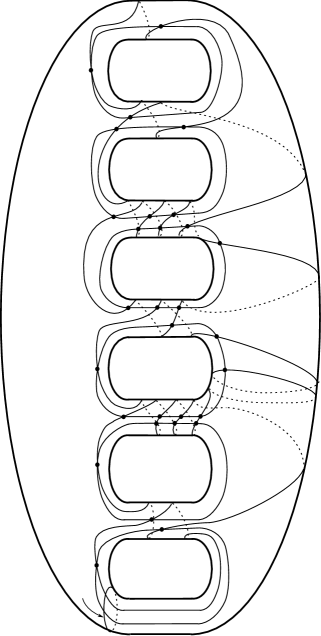
Figure 28: Adapted Heegaard diagram for $L_{1,2}$. The domains (in the complement of the $\alpha$– and $\beta$–circles) labeled by $1,...,10$ play a role in Figure 29.

There are $347$ intersection points, $13$ of which are in the same Alexander grading as ${\bf{x}}_{0}$. In terms of the numbering conventions from Figure 28, these are

$$\begin{array}[]{llll}A_{2}B_{1}C_{3}D_{1}E_{1}F&A_{2}B_{2}C_{2}D_{1}E_{1}F&A_{1}B_{2}C_{4}D_{1}E_{1}F&A_{1}B_{2}C_{1}D_{2}E_{1}F\\ A_{1}B_{1}C_{2}D_{2}E_{1}F&A_{2}B_{2}C_{3}D_{2}E_{1}F&A_{1}B_{2}MVE_{1}F&A_{1}D_{2}E_{1}P_{1}Q_{1}F\\ A_{2}D_{1}E_{1}P_{2}E_{1}F&A_{2}D_{1}E_{1}P_{1}Q_{2}F&A_{2}D_{2}E_{1}P_{2}Q_{2}F&XYC_{3}D_{1}E_{1}F\\ A_{1}B_{1}C_{1}D_{1}E_{1}F={\bf{x}}_{0}.&&&\end{array}$$

We can draw a graph whose vertices consist of these generators, and its arrows denote positive Whitney disks with Maslov index one, as pictured in Figure 29.

Figure 29: Complex for $L_{1,2}$. We have displayed here the $13$ generators in $A=-3$. Arrows represent domains connecting generators. All the thicker arrows actually represent quadrilaterals; there are only four which are not: those containing $1$, and those containing $6+8$.

Those domains are written as sums of the $10$ domains labelled in Figure 28. Note that in that figure, we have abbreviated the names of generators (for example, dropping $F$, which occurs in each). In that picture, all but four of the arrows represent rectangles (and hence, immediately, nontrivial differentials in the chain complex). Inspection of this graph immediately establishes that there are no other non–negative Whitney disks among the given generators with Maslov index one (for example, the domain from $P_{2}Q_{1}=A_{2}D_{1}E_{1}P_{2}Q_{1}F$ to $B_{2}C_{4}=A_{2}B_{2}C_{4}D_{1}E_{1}$ is gotten as $6+3-2+8+6$, which contains $2$ with multiplicity $-1$). To show that $B_{1}C_{1}=A_{1}B_{1}C_{1}D_{1}F$ represents a homologically nontrivial cycle, it suffices to show that the positive domain $6+8$ supports holomorphic representatives, which can be done by direct means. (Note that it is an annulus with an appropriate cut.) ∎

Remark 6.11.

Recall that

$$\mathrm{HFK}^{-}(S^{3},T_{(2,2n-1)})\cong\mathbb{F}^{n-1}\oplus\mathbb{F}[U],$$

where the top generator of the free $\mathbb{F}[U]$–module is at

$$(A=-(n-1),\quad M=-2(n-1)),$$

while the $n-1$ generators of the $\mathbb{F}^{n-1}$ summand are of bi–degrees

$$(A=n-1-2i,\quad M=-2i),\quad i=0,\ldots,n-2.$$

(This follows readily from the calculation of $\widehat{\mathrm{HFK}}$, stated in Equation (6.7).) Once again, the computation above can be adapted to show that the homogeneous $U$–torsion elements ${\mathfrak{L}}(L_{0,l}),{\mathfrak{L}}(L_{1,1})$ and ${\mathfrak{L}}(L_{1,2})$ in $\mathrm{HFK}^{-}(S^{3},T_{(2,2n-1)})$ are also nontrivial.

Notice that there is an obvious bijection between the homogeneous $U$–torsion elements of $\mathrm{HFK}^{-}(S^{3},T_{(2,2n-1)})$ and the Legendrian knots $L_{k,l}$ with $k+l=n-2$ constructed above. Moreover, this bijection can be chosen in such a way that if $L_{k,l}$ corresponds to $x_{k,l}\in\mathrm{HFK}^{-}(S^{3},T_{(2,2n+1)})$ then

$$d_{3}(\xi_{k,l})=2A(x_{k,l})-M(x_{k,l}).$$

It is reasonable to expect that the Legendrian invariants $\widehat{\mathfrak{L}}(L_{k,l})$ and ${\mathfrak{L}}(L_{k,l})$ are nonzero for all $k,l\geq 0$, and hence that ${\mathfrak{L}}(L_{k,l})$ is determined by $x_{k,l}$. We will not address this general computation in the present paper.

7 Connected sums

Suppose that $L_{i}\subset(Y_{i},\xi_{i})$ are oriented Legendrian knots in the contact 3–manifolds $(Y_{i},\xi_{i})$, $i=1,2$. We want to relate the invariants of $L_{1}$ and $L_{2}$ with the invariants of the connected sum $L_{1}\#L_{2}\subset(Y_{1}\#Y_{2},\xi_{1}\#\xi_{2})$ (see [14] for the definition of the connected sum operation in the contact setting).

Fix open book decompositions $(B_{i},\varphi_{i})$ adapted to $L_{i}\subset(Y_{i},\xi_{i})$ (with pages $S_{i}$) for $i=1,2$. We may assume that suitable portions of the open books and the adapted bases appear as in the left–hand picture of Figure 30, where, as usual, the ordered pairs $(z_{i},w_{i})$ determine the orientations of the knots. We can now perform the Legendrian connected sum of $(Y_{1},\xi_{1},L_{1})$ and $(Y_{2},\xi_{2},L_{2})$ in such a way that we glue the open books as well as the contact structures and the knots. Specifically, we take the Murasugi sum of the two open books in the domains containing $z_{2}$ and $w_{1}$, and then we drop these two basepoints. We can make sure that the resulting oriented knot $L_{1}\#L_{2}$ is smoothly determined on a page of the resulting open book by the ordered pair $(z_{1},w_{2})$, as illustrated in the central picture of Figure 30. The bases of arcs can also be arranged to be the same as the ones illustrated.

There is a corresponding map of chain complexes

$$\Phi\colon\mathrm{CFK}^{-}(-Y_{1},L_{1})\otimes_{\mathbb{F}[U]}\mathrm{CFK}^{-}(-Y_{2},L_{2})\to\mathrm{CFK}^{-}(-(Y_{1}\#Y_{2}),L_{1}\#L_{2})$$ (7.1)

which (denoting the intersection point determining ${\mathfrak{L}}(L_{i})$ by ${\bf{x}}(L_{i})$) maps the intersection point ${\bf{x}}(L_{1})\otimes{\bf{x}}(L_{2})$ to the generator $({\bf{x}}(L_{1}),{\bf{x}}(L_{2}))$ of the chain complex of the connected sum. According to [35, Section 7] the above map induces an isomorphism on homology. The union of the two bases is not adapted to the Legendrian knot $L_{1}\#L_{2}$, since each of the two bases contains an arc intersecting it. Nevertheless, as it will be shown in the proof of Theorem 7.1, there is a sequence of arc slides which carries the new basis of curves into an adapted basis for $L_{1}\#L_{2}$, inducing handleslides on the underlying Heegaard diagram for $(-(Y_{1}\#Y_{2}),L_{1}\#L_{2})$. These handleslides induce a map of chain complexes by counting holomorphic triangles (cf. [33, Section 9])

$$\Psi\colon\mathrm{CFK}^{-}(-(Y_{1}\#Y_{2}),L_{1}\#L_{2})\longrightarrow\mathrm{CFK}^{-}(-(Y_{1}\#Y_{2}),L_{1}\#L_{2}),$$

where the second chain complex now denotes the chain complex with respect to the adapted Heegaard diagram.

Theorem 7.1.

Suppose that $L_{1}\#L_{2}\subset(Y_{1}\#Y_{2},\xi_{1}\#\xi_{2})$ is the oriented connected sum of the oriented Legendrian knots $L_{i}\subset(Y_{i},\xi_{i})$, $(i=1,2)$. Then, there is a quasi–isomorphism

$$F\colon\mathrm{CFK}^{-}(-Y_{1},L_{1})\otimes_{\mathbb{F}[U]}\mathrm{CFK}^{-}(-Y_{2},L_{2})\to\mathrm{CFK}^{-}(-(Y_{1}\#Y_{2}),L_{1}\#L_{2})$$

which maps ${\bf{x}}(L_{1})\otimes{\bf{x}}(L_{2})$ to ${\bf{x}}(L_{1}\#L_{2})$.

Proof.

There are three Heegaard diagrams for $(-(Y_{1}\#Y_{2}),L_{1}\#L_{2})$ coming into play: the connected sum diagram (whose $\mathbb{\alpha}$– and $\mathbb{\beta}$–circles are gotten by doubling the initial bases), an intermediate diagram gotten by sliding the $\alpha$-circles as dictated by the arcslides in the middle diagram in Figure 30 (whose attaching circles we denote $\alpha^{\prime}$ and $\beta$), and the final one gotten by performing handleslides on the $\beta$-circles, as dictated by arcslides of the $b_{i}$ as in the rightmost diagram in Figure 30 (whose attaching cicles are $\alpha^{\prime}$ and $\beta^{\prime}$). Recall, that the $a_{i}$ arcs determine the $\alpha$–circles while the $b_{i}$’s give rise to the $\beta$–circles, and we are examining the Heegaard diagrams $(\Sigma,\beta,\alpha),(\Sigma,\beta,\alpha^{\prime})$ and $(\Sigma,\beta^{\prime},\alpha^{\prime})$.

2pt $z_{1}$ at 20 40 $z_{2}$ at 20 114 $a_{2}$ at 35 15 $b_{2}$ at 61 14 $w_{1}$ at 47 51 $w_{2}$ at 43 105 $b_{1}$ at 32 142 $a_{1}$ at 56 143

$b_{2}$ at 184 12 $a_{2}$ at 135 10 $a^{\prime}_{2}$ at 146 11 $b_{1}$ at 180 115 $a_{1}$ at 205 124 $a^{\prime}_{1}$ at 192 119 $z_{1}$ at 121 34 $w_{2}$ at 208 77

$b_{2}$ at 319 9 $b^{\prime}_{2}$ at 299 8 $a^{\prime}_{2}$ at 282 8 $b_{1}$ at 315 110 $b^{\prime}_{1}$ at 329 116 $a^{\prime}_{1}$ at 340 120 $z_{1}$ at 260 28 $w_{2}$ at 341 71

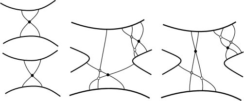
Figure 30: Connected sums. Starting from two knots as pictured on the left, we form their connected sum to obtain a Heegaard diagram as in the middle, where we have three sets of arcs, two sets of which are isotopic to one another, and the third is obtained as an arcslide. In the middle picture, the dark dots represent the initial generator ${\bf{x}}$ (which represents the product of the two Legendrian invariants), the white dots represent the canonical generator for $\mathbb{T}_{\alpha}\cap{\mathbb{T}}_{\alpha^{\prime}}$, and the grey dots represent the intermediate generator ${\bf{x}}^{\prime}$; whereas on the picture on the right, the dark dots represent ${\bf{x}}^{\prime}$, the white dots represent the canonical generator of $\mathbb{T}_{\beta}\cap{\mathbb{T}}_{\beta^{\prime}}$, and the grey dots represent the final intersection point ${\bf{x}}^{\prime\prime}$ (which represents the Legendrian invariant for the connected sum).

In all three of these diagrams there is a unique intersection point of the $\alpha$– and $\beta$–tori which is supported in $S_{+1}$: the first, ${\bf{x}}$, represents the product of ${\bf{x}}(L_{1})$ and ${\bf{x}}(L_{2})$ under the connected sum map (denoted above by $\Phi$), the second is denoted ${\bf{x}}^{\prime}$, and the third, ${\bf{x}}^{\prime\prime}$, clearly determines the Legendrian invariant for $L_{1}\#L_{2}$. We claim that the three generators are mapped to one another under the maps induced by handleslides.

As a warm-up, we argue first that ${\bf{x}}^{\prime}$ is, indeed, a cycle. As for the contact class, we argue that for any ${\bf{y}}\in{\mathbb{T}}_{\beta^{\prime}}\cap\mathbb{T}_{\alpha}$, if $\phi\in\pi_{2}({\bf{x}}^{\prime},{\bf{y}})$ is any Whitney disk with all non–negative local multiplicities, then ${\bf{x}}^{\prime}={\bf{y}}$ and $\phi$ is the constant disk. The argument is similar to the argument from [19] recalled in the proof of Theorem 2.11 with one slight difference: now the arcs in the basis disconnect $S_{+1}$ into two regions, only one of which contains $z$. However, it is still easy to see (by another look at Figure 30) that any postive domain flowing out of ${\bf{x}}^{\prime}$ which has positive multiplicity on the other region (not containing $z$) must also have positive multiplicity at $z$.

We now turn to the verification of the claim about the triangle maps. The Heegaard triple in this case is $(\Sigma,\beta,\alpha,\alpha^{\prime},w,z)$, and the diagram $(\Sigma,\alpha,\alpha^{\prime},w,z)$ represents an unknot in the $g$–fold connected sum of $S^{2}\times S^{1}$. Moreover, in that diagram there is a unique intersection point $\Theta\in\mathbb{T}_{\alpha}\cap{\mathbb{T}}_{\alpha^{\prime}}$ representing the top–dimensional Floer homology class. The handleslide map

$$\Psi_{1}\colon\mathrm{CFK}^{-}(\Sigma,\beta,\alpha,w,z)\longrightarrow\mathrm{CFK}^{-}(\Sigma,\beta,\alpha^{\prime},w,z)$$

is defined by

$$\Psi_{1}({\mathbf{u}})=\sum_{{\bf{y}}\in\mathbb{T}_{\beta}\cap{\mathbb{T}}_{\alpha^{\prime}}}\sum_{\{\psi\in\pi_{2}({\mathbf{u}},\Theta,{\bf{y}})\big{|}\mu(\psi)=0,n_{z}(\psi)=0\}}\#{\mathfrak{M}}(\psi)\cdot U^{n_{w}(\psi)}{\bf{y}},$$

where, as usual, $\pi_{2}({\mathbf{u}},\Theta,{\bf{y}})$ denotes the space of homology classes of Whitney triangles at ${\mathbf{u}}$, $\Theta$, and ${\bf{y}}$.

The claim that $\Psi_{1}({\bf{x}})={\bf{x}}^{\prime}$ follows from the facts that

• there is a triangle $\psi_{0}\in\pi_{2}({\bf{x}},\Theta,{\bf{x}}^{\prime})$, gotten as a disjoint union of the obvious small triangles in $S_{+1}$, and

• any other triangle $\psi\in\pi_{2}({\bf{x}},\Theta,{\bf{y}})$ with $n_{z}(\psi)=0$ has a negative local multiplicity somewhere.

The first is gotten by glancing at Figure 30. To see the second, notice that any homology class $\psi\in\pi_{2}({\bf{x}}^{\prime},\Theta,{\bf{y}})$ can be decomposed as $\psi_{0}*\phi$, where $\phi\in\pi_{2}({\bf{x}}^{\prime},{\bf{y}})$. Moreover, if $\psi$ has only positive local multiplicities, then the same follows for $\phi$; also, since $n_{z}(\psi)=0=n_{z}(\psi_{0})$, it follows that $n_{z}(\phi)=0$, as well. But by our above argument that ${\bf{x}}^{\prime}$ is a cycle, it now follows that $\phi$ is constant.

Consider next the handleslide map

$$\Psi_{2}\colon(\Sigma,\beta,\alpha^{\prime},w,z)\longrightarrow(\Sigma,\beta^{\prime},\alpha^{\prime},w,z).$$

This is defined by pairing with an intersection point ${\Theta^{\prime}}\in{\mathbb{T}}_{\beta^{\prime}}\cap\mathbb{T}_{\beta}$ representing the top–dimensional nontrivial homology. The argument that $\Psi_{2}({\bf{x}}^{\prime})={\bf{x}}^{\prime\prime}$, where ${\bf{x}}^{\prime\prime}$ determines the Legendrian invariant for the connected sum, follows through a similar argument.

The composition $\Psi_{2}\circ\Psi_{1}\circ\Phi$ now induces an isomorphism on homology, carrying ${\bf{x}}(L_{1})\otimes{\bf{x}}(L_{2})$ to ${\bf{x}}(L_{1}\#L_{2})$, which completes the proof of the theorem. ∎

The above result quickly leads to the following observation, providing

Proof of Theorem 1.6.

Interpret stabilization as the connected sum with the stabilized Legendrian unknot in the standard contact 3–sphere, use the connected sum formula and the model calculation given in Section 4. This gives quasi–isomorphisms

$$\Psi^{-}\colon\thinspace\mathrm{CFK}^{-}(-Y,L)\to\mathrm{CFK}^{-}(-Y,L^{-})$$

and

$$\Psi^{+}\colon\thinspace\mathrm{CFK}^{-}(-Y,L)\to\mathrm{CFK}^{-}(-Y,L^{+})$$

such that

$$\Psi^{-}({\bf{x}}(L))={\bf{x}}((L^{-})\quad\text{and}\quad U\cdot\Psi^{+}({\bf{x}}(L))={\bf{x}}(L^{+}),$$

concluding the proof of the theorem. ∎

Note that Proposition 5.2 is a special case of Theorem 1.6; we gave a separate proof of it earlier, since that proof is somewhat more direct. As an application of our previous computations we can now prove the following result:

Theorem 7.2.

Let $\xi_{i}$ denote the overtwisted contact structure on $S^{3}$ with Hopf invariant $d_{3}(\xi_{i})=i\in{\mathbb{Z}}$. Then, $\xi_{i}$ contains non–loose Legendrian knots with non–vanishing Legendrian invariants $\widehat{\mathfrak{L}}$ for each $i\in{\mathbb{Z}}$.

Proof.

By Proposition 6.4 and Lemma 6.1, for $i>0$ even the Legendrian knot $L_{0,i-1}$, while for $i<0$ odd the knot $L(i)$ satisfies the claim. If $i=2j-1>0$ is odd then by the connected sum formula $L_{0,j-1}\#L(1)$ is a good choice. For $i=2j<0$ even take $L(j)\#L(1)$ and finally for $i=0$ the knot $L_{0,0}\#L(1)\#L(1)$ will do. ∎

Corollary 7.3.

Suppose that $(Y,\xi)$ is a contact 3–manifold with nonvanishing contact invariant $c(Y,\xi)$ and $\zeta$ is an overtwisted contact structure on $Y$ with $\mathbf{t}_{\zeta}=\mathbf{t}_{\xi}$. Then $(Y,\zeta)$ contains Legendrian (transverse) knots with nonvanishing Legendrian (resp. transverse) invariants.

Proof.

Consider a Legendrian unknot $L$ (in a Darboux chart) in $(Y,\xi)$ with $c(Y,\xi)\neq 0$. It is not difficult to find, possibly after stabilization, an open book decomposition compatible with $(Y,\xi,L)$ together with an adapted basis, in such a way that the two basepoints $z$ and $w$ determining $L$ are, in fact, in the same domain. This observation immediately implies $\widehat{\mathrm{HFK}}(-Y,L)=\widehat{\mathrm{HF}}(-Y)$, and the Legendrian invariant $\widehat{\mathfrak{L}}$ of $L$ is easily seen to be nonzero in $\widehat{\mathrm{HFK}}(-Y,L)$, being equal to $c(Y,\xi)$. Any overtwisted contact structure $\zeta$ on $Y$ with $\mathbf{t}_{\zeta}=\mathbf{t}_{\xi}$ can be given as $\xi\#\xi_{i}$, where $\xi_{i}$ is the overtwisted contact structure on $S^{3}$ with $d_{3}(\xi_{i})=i$. This fact easily follows from Eliashberg’s classification of overtwisted contact structures, together with the classification of homotopy types of 2–plane fields. Now the connected sum of the Legendrian unknot with the Legendrian knot having nontrivial Legendrian knot invariant in $\xi_{i}$ (provided by Theorem 7.2) has nontrivial Legendrian invariant by the connected sum formula. This knot, and each of its negative stabilizations are non–loose, and hence its transverse push–off is non–loose and has nontrivial transverse invariant. ∎

8 Transversely non–simple knots

A knot type $\mathcal{K}$ in $S^{3}$ is traditionally called transversely simple if two transverse knots $T_{1},T_{2}$ in the standard contact structure $\xi_{st}$ both of knot type $\mathcal{K}$ and equal self–linking number are transversely isotopic. Transversely non–simple knot types were recently found by Etnyre-Honda, Birman-Menasco [15, 1], cf. also [29, 44].

The notion of transverse simplicity obviously generalizes to any null–homologous knot type (for the self–linking number to be well–defined) in any contact 3–manifold $(Y,\xi)$. In this form of the definition, however, it is easy to find transversely non–simple knot types provided $\xi$ is overtwisted: The binding of any open book decomposition compatible with $\xi$ is a null–homologous, non–loose transverse knot, while the same binding in $(Y\#S^{3},\xi\#\xi_{0})$ (where $\xi_{0}$ is the overtwisted contact structure on $S^{3}$ homotopic to $\xi_{st}$ and the connected sum is taken away from the binding) is loose. Since $\xi$ and $\xi\#\xi_{0}$ are homotopic as 2–plane fields, hence isotopic as contact structures, the binding gives rise to two transverse knots in $\xi$. The self–linking numbers of these two representatives are clearly equal, while one has tight, the other overtwisted complement; consequently the two knots cannot be transversely isotopic. In conclusion, for overtwisted contact structures in the definition of transverse simplicity we should require that the two knots are either both non–loose or both loose (besides being smoothly isotopic and having identical self–linking). Two transverse loose knots with equal knot type and self–linking number, and with a common overtwisted disk in their complement can be shown to be isotopic. Without the existence of the common overtwisted disk, however, this question is surprisingly subtle.

With the aid of the transverse invariant $\mathfrak{T}$ and the model calculations for $L_{1,1}$ and $L_{1,2}$ discussed in the previous section (together with a refinement of the gradings on Heegaard Floer homology, deferred to Section 9) we get

Theorem 8.1.

Let ${\mathcal{K}}$ denote the knot type obtained by the connected sum of the negative torus knots $T_{(2,-7)}$ and $T_{(2,-9)}$. Then, in the overtwisted contact 3–manifold $(S^{3},\xi_{12})$ with Hopf invariant $d_{3}(\xi_{12})=12$ there are two non–loose Legendrian knots representing ${\mathcal{K}}$, with equal Thurston–Bennequin and rotation numbers, which are not Legendrian isotopic and stay nonisotopic after arbitrarily many negative stabilizations.

The proof of Theorem 8.1 proceeds by considering a pair of appropriate Legendrian representatives of ${\mathcal{K}}$, the computation of their invariants, and finally the distinction of these elements. Our candidate Legendrian knots are

$$L_{1}=L_{0,2}\#L_{1,2}\quad{\mbox{and}}\quad L_{2}=L_{1,1}\#L_{0,3}.$$

The knots $L_{1}$ and $L_{2}$ are obviously smoothly isotopic to $T_{(2,-7)}\#T_{(2,-9)}$, and their Thurston–Bennequin and rotation numbers can be easily deduced from their definition:

Lemma 8.2.

The Thurston–Bennequin and rotation numbers of $L_{1}$ and $L_{2}$ are

$$\operatorname{tb}(L_{1})=\operatorname{tb}(L_{2})=-31\quad{\mbox{and}}\quad\operatorname{rot}(L_{1})=\operatorname{rot}(L_{2})=-40,$$

with the orientations specified by Figure 17.

Proof.

The formulae follow from the additivity of rotation numbers and the identity

$$\operatorname{tb}(L\#L^{\prime})=\operatorname{tb}(L)+\operatorname{tb}(L^{\prime})+1$$

(cf. [14, Lemma 3.3]), together with the computations of Lemma 6.7. ∎

Since $L_{1}$ and $L_{2}$ are knots in the connected sums of the corresponding overtwisted contact structures, the claim about the resulting contact structure follows. (Recall that on $S^{3}$ an overtwisted contact structure is determined up to isotopy by its Hopf invariant, which is additive under connected sum.) The connected sum formula of Theorem 7.1 implies that the Legendrian invariant of both knots is determined by the tensor product of the invariants of the summands. This argument shows that $\widehat{\mathfrak{L}}(L_{1})$ and $\widehat{\mathfrak{L}}(L_{2})$ are non–vanishing, hence the knots $L_{1},L_{2}$ are both non–loose. (Notice that, in general, the connected sum of two non–loose knots might become loose.) The connected sum formula for knot Floer homology shows that in the Alexander and Maslov grading $(A=5,M=-2)$ of the elements $\widehat{\mathfrak{L}}(L_{i})$ the knot Floer homology group $\widehat{\mathrm{HFK}}(S^{3},T_{(2,7)}\#T_{(2,9)})$ is isomorphic to $\mathbb{F}\oplus\mathbb{F}\oplus\mathbb{F}$. (Only $\mathbb{F}\oplus\mathbb{F}$ comes from the $\mathrm{HFK}^{-}$–theory, hence capable of containing $\widehat{\mathfrak{L}}$.) Therefore to conclude our proof for Theorem 8.1 we need to show that the knots $L_{1}$ and $L_{2}$ are not isotopic. This step requires an auxiliary result from knot Floer homology, showing that elements of the knot Floer group of a connected sum do remember the Alexander and Maslov gradings of their components in the summands. This leads to a refinement of the invariant, which we explain now. (The necessary Heegaard Floer theoretic result will be given in Section 9.)

Recall that the invariant ${\mathfrak{L}}(L)$ was defined as an element of $\mathrm{HFK}^{-}(-Y,L)$, determined up to any $\mathbb{F}[U]$–module isomorphism of this module. The ambiguity stems from the fact that for (oriented) Legendrian isotopic knots $L_{1},L_{2}$ the isotopy is not canonical, therefore the isomorphism between the knot Floer homologies $\mathrm{HFK}^{-}(-Y,L_{1})$ and $\mathrm{HFK}^{-}(-Y,L_{2})$ will depend on the chosen isotopy. To prove vanishing and non–vanishing results, it was sufficient to mod out by all the module automorphisms. When we want to distinguish knots based on their invariants, however, we might need to understand the necessary equivalence relations a little better. Notice that an isotopy between $L_{1}$ and $L_{2}$ induces a filtered chain homotopy between the filtered chain complexes $\mathrm{CFK}^{-}(-Y,L_{i})$ (where the filtration comes from the second basepoint), hence any algebraic structure of the filtered chain complex provides further restrictions on the automorphisms of $\mathrm{HFK}^{-}(-Y,L)$ we need to take into account for the invariance property to hold. For example, the length of a homogeneous element $x$ (that is, the minimal $n$ for which $d_{n}(x)$ vanishes, where $d_{n}$ is the $n^{th}$ higher derivative on the spectral sequence associated to the filtered chain complex $\mathrm{CFK}^{-}(-Y,L)$) is such a further structure, as it is exploited in [29]. In a slightly different direction, in [31] two of the authors of the present paper have shown that the mapping class group

$${\rm{MCG}}(Y,L)={\rm{Diff}}^{+}(Y,L)/{\rm{Diff}}^{+}_{0}(Y,L)$$

of the complement of the knot admits a natural action on $\mathrm{HFK}^{-}(-Y,L)$, and it is not hard to see that the Legendrian invariant can be defined as an orbit of the action of ${\rm{MCG}}(Y,L)$ rather than of the full automorphism group. In many cases the mapping class group of a knot is relatively small, hence this refinement provides a significant sharpening of the invariant — without even understanding the explicit action of the mapping class group on the knot Floer homologies. In some cases, however, the mapping class group can be large (although might admit a fairly trivial representation on the Floer homology), in which case the description of the action cannot be avoided. For example, connected sums of knots have infinite mapping class groups.

For connected sums, therefore, we describe a slightly different refinement of the invariant. For the sake of simplicity, we will be content with formulating the relevant results for the $\widehat{\mathrm{HFK}}$–theory only.

Definition 8.3.

The $\mathbb{F}$–vector space $M=\oplus_{s}M_{*}(s)$ is Alexander bigraded if it admits a splitting

$$M=\oplus_{s}(\oplus_{\{s_{1},s_{2}\mid s_{1}+s_{2}=s\}}M_{*}(s_{1},s_{2})).$$

The pair $(M,m)$ of an Alexander bigraded vector space $M$ and an element $m\in M$ defines an equivalence class $[[M,m]]$ of such objects by saying that $(M,m)$ and $(N,n)$ are equivalent if there is an isomorphism $f\colon M\to N$ with the property that $f(m)=n$ and $f(M_{*}(s_{1},s_{2}))=N(s_{1},s_{2})$. In other words, we require the isomorphisms to respect the Alexander bigrading of the vector space.

For a null–homologous Legendrian knot $L$ in the contact 3–manifold $(Y,\xi)$ consider the homology class $\alpha_{\widehat{\mathfrak{L}}}(L)\in\widehat{\mathrm{HFK}}(-Y,L,\mathbf{t}_{\xi})$ given by the cycle ${\bf{x}}(B,\varphi,A)$ as in Definition 3.4. By slightly modifying the definition of Theorem 1.1, consider

$${\widetilde{{\mathfrak{L}}}}(L):=[[\widehat{\mathrm{HFK}}(-Y,L,\mathbf{t}_{\xi}),\alpha_{\widehat{\mathfrak{L}}}(L)]].$$

Theorem 8.4.

Suppose that $L$ is a given null–homologous Legendrian knot in the contact 3–manifold $(Y,\xi)$ representing the knot type ${\mathcal{K}}$, which is the connected sum of two knot types ${\mathcal{K}}_{1}$ and ${\mathcal{K}}_{2}$. Then for any knot $K$ of type ${\mathcal{K}}$ the knot Floer homology $\widehat{\mathrm{HFK}}(-Y,K)$ naturally admits an Alexander bigrading and ${\widetilde{{\mathfrak{L}}}}(L)$ is an invariant of its oriented Legendrian isotopy class. In particular, if $L,L^{\prime}$ are two Legendrian representatives of ${\mathcal{K}}$ and ${\widetilde{{\mathfrak{L}}}}(L)\neq{\widetilde{{\mathfrak{L}}}}(L^{\prime})$ then $L$ and $L^{\prime}$ are not Legendrian isotopic.

Proof.

The Künneth formula [35] provides an Alexander bigrading for the knot Floer homology of $K=K_{1}\#K_{2}$ by using the Alexander gradings of the knot Floer groups of $K_{1}$ and $K_{2}$. Theorem 9.1 now shows that the map $f_{1}$ appearing in the proof of Corollary 3.6 induces an isomorphism on the knot Floer homology which respects this Alexander bigrading. Therefore the proof of the corollary, in fact, shows that for connected sums the refined equivalence class ${\widetilde{{\mathfrak{L}}}}(L)$ is an invariant of the Legendrian isotopy class of $L$. ∎

Proof of Theorem 8.1.

As we saw above, the Legendrian knots $L_{1}$ and $L_{2}$ both represent the knot type of ${\mathcal{K}}$, and have equal Thurston–Bennequin invariants and rotation numbers. Now

$$\widehat{\mathrm{HFK}}(S^{3},m(K),5)=\widehat{\mathrm{HFK}}(S^{3},T_{(2,7)},3)\otimes\widehat{\mathrm{HFK}}(S^{3},T_{(2,9)},2)\oplus$$

$$\widehat{\mathrm{HFK}}(S^{3},T_{(2,7)},2)\otimes\widehat{\mathrm{HFK}}(S^{3},T_{(2,9)},3)\oplus\widehat{\mathrm{HFK}}(S^{3},T_{(2,7)},1)\otimes\widehat{\mathrm{HFK}}(S^{3},T_{(2,9)},4),$$

and the cycle which determines $\widehat{\mathfrak{L}}(L_{1})$ is in the first summand, while the cycle which determines $\widehat{\mathfrak{L}}(L_{2})$ is in the last. (The image of the quotient map from $\mathrm{HFK}^{-}$ to $\widehat{\mathrm{HFK}}$, which contains ${\widehat{\mathfrak{L}}}$, is disjoint from the middle summand.) In other words, the Alexander bigrading of $\widehat{\mathfrak{L}}(L_{1})$ is $(3,2)$, while for $\widehat{\mathfrak{L}}(L_{2})$ this quantity is $(1,4)$. This readily implies that the refined invariants ${\widetilde{{\mathfrak{L}}}}(L_{1})$ and ${\widetilde{{\mathfrak{L}}}}(L_{2})$ are distinct, and so by Theorem 8.4 the knots $L_{1}$ and $L_{2}$ are not Legendrian isotopic. ∎

Proof of Theorem 1.7.

Let $K$ denote the connected sum $T_{(2,-7)}\#T_{(2,-9)}$. Consider the positive transverse push–offs $T_{1}$ and $T_{2}$ of the Legendrian knots $L_{1}$ and $L_{2}$. By defining the refined transverse invariant ${\tilde{\mathfrak{T}}}(T_{i})$ as ${\tilde{{\mathfrak{L}}}}(L_{i})$, the proof of Theorem 8.1 implies that $T_{1}$ and $T_{2}$ are transversely nonisotopic. Since their self–linking numbers $s\ell(T_{i})$ can be easily computed from the Thurston–Bennequin and rotation numbers of the Legendrian knots $L_{i}$, we get that $s\ell(T_{1})=s\ell(T_{2})$. Therefore $K$ as defined above is a transversely non–simple knot type in the overtwisted contact structure $\xi_{12}$, concluding the proof. ∎

Notice that if the nontriviality of the Legendrian invariants of all Legendrian knots $L_{i,j}$ can be established, the argument used in the proof of Theorem 1.7 actually provides arbitrarily many transversely distinct transverse knots with the same classical invariants: consider the connected sums

$$L_{i,j}\#L_{k,l}$$

with $i+j=n-2$ and $k+l=m-2\geq n-2$ fixed (hence fixing the knot type and the Thurston–Bennequin numbers of the knots) and take only those knots which satisfy $i+k=n-2$. It is not hard to see that these knots will have the same rotation numbers, but the argument given in the proof of Theorem 1.7, assuming that the invariants for the $L_{i,j}$ are nontrivial, shows that the transverse invariants of their positive transverse push–offs do not agree. This would be a way of constructing arbitrarily many distinct transverse knots with the same classical invariants in some overtwisted contact $S^{3}$.

Proof of Corollary 1.8..

Consider the overtwisted contact structure $\zeta$ on $Y$ with $\mathbf{t}_{\zeta}=\mathbf{t}_{\xi}$ and write it as $\zeta^{\prime}\#\xi_{12}$, where $\zeta^{\prime}$ is an overtwisted contact structure on $Y$ with $\mathbf{t}_{\zeta^{\prime}}=\mathbf{t}_{\xi}$. (Again, by simple homotopy theoretic reasons and the classification of overtwisted contact structures, the above decomposition is possible.) The connected sum of the Legendrian knot $L$ in $\zeta^{\prime}$ having nontrivial invariant ${\tilde{{\mathfrak{L}}}}(L)$ with $L_{1}$ and $L_{2}$ of Theorem 1.7 obviously gives a pair of Legendrian knots with equal classical invariants in $\zeta$, but with the property that their transverse push–offs have distinct transverse invariants. The distinction of these elements relies on a straightforward modification of Theorem 9.1, where the components in a fixed connected sum decomposition are not necessarily prime knots, but we fix the isotopy class of the embedded sphere separating the knot into two connected components. This construction concludes the proof. ∎

9 Appendix: On knot Floer homology of connected sums

Recall from [35] that if $(Y_{1},K_{1})$ and $(Y_{2},K_{2})$ are two three–manifolds equipped with knots, then we can form their connected sum $(Y_{1}\#Y_{2},K_{1}\#K_{2})$. In this case, the knot Floer homology for the connected sum can be determined by the knot Floer homology of its summands by a Künneth formula. Our aim here is to investigate naturality properties of this decomposition. Specifically, we prove the following

Theorem 9.1.

Let $K$ be a knot obtained as a connected sum of two distinct prime knots $K_{1}$ and $K_{2}$. Then there is an additional intrinsic grading on the knot Floer homology of $K$ with the property that

$$\widehat{\mathrm{HFK}}(K,s)=\bigoplus_{\{s_{1},s_{2}\big{|}s_{1}+s_{2}=s\}}\widehat{\mathrm{HFK}}(K,s_{1},s_{2}),$$

where $\widehat{\mathrm{HFK}}(K,s_{1},s_{2})=\widehat{\mathrm{HFK}}(K_{1},s_{1})\otimes\widehat{\mathrm{HFK}}(K_{2},s_{2})$. More precisely, if $D(K_{1})$ and $D(K_{2})$ are diagrams for $K_{1}$ and $K_{2}$ respectively, then there is an induced diagram $D(K_{1})\#D(K_{2})$ for $K_{1}\#K_{2}$, together with an isomorphism

$$\Phi\colon H_{*}(\widehat{\mathrm{CFK}}(D(K_{1})))\otimes H_{*}(\widehat{\mathrm{CFK}}(D(K_{2})))\longrightarrow H_{*}(\widehat{\mathrm{CFK}}(D(K_{1})\#D(K_{2}))).$$

If $D^{\prime}(K_{1})$ and $D^{\prime}(K_{2})$ are a pair of different diagrams for $K_{1}$ and $K_{2}$, and $D^{\prime}(K_{1})\#D^{\prime}(K_{2})$ denotes the induced sum of diagrams for $K_{1}\#K_{2}$, then there is an isomorphism $\Psi\colon H_{*}(\widehat{\mathrm{CFK}}(D(K_{1})\#D(K_{2})))\longrightarrow H_{*}(\widehat{\mathrm{CFK}}(D^{\prime}(K_{1})\#D^{\prime}(K_{2})))$ such that the diagram

$$\begin{CD}H_{*}(\widehat{\mathrm{CFK}}(D(K_{1})))\otimes H_{*}(\widehat{\mathrm{CFK}}(D(K_{2})))@>{\Phi}>{}>H_{*}(\widehat{\mathrm{CFK}}(D(K_{1})\#D(K_{2})))\\ @V{\psi_{1}\otimes\psi_{2}}V{}V@V{\Psi}V{}V\\ H_{*}(\widehat{\mathrm{CFK}}(D^{\prime}(K_{1})))\otimes H_{*}(\widehat{\mathrm{CFK}}(D^{\prime}(K_{2})))@>{\Phi^{\prime}}>{}>H_{*}(\widehat{\mathrm{CFK}}(D^{\prime}(K_{1})\#D^{\prime}(K_{2})))\end{CD}$$ (9.1)

commutes.

Let $Y$ be a closed, oriented three–manifold, $K\subset Y$ be an oriented knot, and $S\subset Y$ meeting $K$ transversely in exactly two points. Call $S$ a splitting sphere for $K$. A splitting sphere expresses $K$ as a connected sum of two knots $K_{1}$ and $K_{2}$. In the case where one of the two summands is unknotted, we call the splitting sphere trivial. In this language, a knot $K$ is prime if every splitting sphere for $K$ is trivial. Recall the following classical result [22].

Theorem 9.2.

If $K$ is the connected sum of two prime knots $K_{1}$ and $K_{2}$, then there is, up to isotopy, a unique nontrivial splitting sphere $S$ for $K$. ∎

Let $(\Sigma,\mathbb{\alpha},\mathbb{\beta},w,z,\gamma)$ be a doubly-pointed Heegaard diagram equipped with a curve $\gamma\subset\Sigma$ which is disjoint from all $\alpha_{i}$, $\beta_{j}$, $w$, and $z$. Suppose moreover that $\gamma$ is a separating curve, dividing $\Sigma$ into two components $F_{1}$ and $F_{2}$, so that $w\in F_{1}$ and $z\in F_{2}$. This decorated Heegaard diagram determines the following data:

• a three–manifold $Y$ (gotten from the Heegaard diagram)

• an oriented knot $K\subset Y$ (determined by $w$ and $z$)

• an embedded two–sphere $S$ meeting the Heegaard surface along $\gamma$ (consisting of all Morse flows between index zero and index three critical points passing through $\gamma$);

i.e. a decorated Heegaard diagram determines a knot $K$ in $Y$ together with a splitting sphere $S$. We call $(\Sigma,\mathbb{\alpha},\mathbb{\beta},w,z,\gamma)$ a decorated Heegaard diagram compatible with $(Y,K,S)$.

Definition 9.3.

A decorated Heegaard move on $(\Sigma,\mathbb{\alpha},\mathbb{\beta},w,z,\gamma)$ is a move of one of the following types:

• Isotopies. Isotopies of $\mathbb{\alpha}$ and $\mathbb{\beta}$, preserving the conditions that all curves among the $\mathbb{\alpha}$ and $\mathbb{\beta}$ are disjoint, and disjoint from $w$, $z$, and $\gamma$; isotopy of $\gamma$, preserving the condition that it is disjoint from $\mathbb{\alpha}$, $\mathbb{\beta}$, $w$, and $z$.

• Handleslides. Handleslides among the $\mathbb{\alpha}$ or $\mathbb{\beta}$, supported in the complement of $w$, $z$, and away from $\gamma$.

• Stabilizations/destabilizations. Stabilization is obtained by forming the connected sum of $(\Sigma,\mathbb{\alpha},\mathbb{\beta},w,z,\gamma)$ with a genus one surface equipped with a pair of curves $\alpha_{g+1}$ and $\beta_{g+1}$ meeting transversely in a single point; destabilization is the inverse operation.

Proposition 9.4.

Suppose that $(\Sigma,\mathbb{\alpha},\mathbb{\beta},w,z,\gamma)$ and $(\Sigma^{\prime},\mathbb{\alpha}^{\prime},\mathbb{\beta}^{\prime},w^{\prime},z^{\prime},\gamma^{\prime})$ are two decorated Heegaard diagrams compatible with $(Y,K,S)$ and $(Y^{\prime},K^{\prime},S^{\prime})$ respectively. If $(Y,K,S)$ is diffeomorphic to $(Y^{\prime},K^{\prime},S^{\prime})$, then the decorated Heegaard diagram $(\Sigma^{\prime},\mathbb{\alpha}^{\prime},\mathbb{\beta}^{\prime},w^{\prime},z^{\prime},\gamma^{\prime})$ is diffeomorphic to one obtained from $(\Sigma,\mathbb{\alpha},\mathbb{\beta},w,z,\gamma)$ after a finite sequence of decorated Heegaard moves.

Proof.

Fix a Morse function $f_{0}$ compatible with $(\Sigma,\mathbb{\alpha},\mathbb{\beta},w,z,\gamma)$. Let $f_{1}$ be a different Morse function compatible with $(\Sigma,\mathbb{\alpha},\mathbb{\beta},w,z,\gamma)$, which agrees with $f_{0}$ in a neighborhood of $S\cup K$. Then we can connect them by a generic one-parameter family $f_{t}$, wherein they undergo isotopies, handleslides and stabilizations/destabilizations. Since all functions have the prescribed behavior at $w$, $z$, and $\gamma$, the Heegaard moves will be supported away from $w$, $z$, and $\gamma$. Changing $f$ near $S\cup K$ has the effect of isotopies of $\Sigma$ supported near $w$, $z$, and $\gamma$. ∎

Proof of Theorem 9.1.

Let $(\Sigma,\mathbb{\alpha},\mathbb{\beta},w,z,\gamma)$ be a Heegaard diagram for $K=K_{1}\#K_{2}$. Then, our additional grading is defined (up to an additive constant) as follows. Fix a point $m$ near $\gamma$. We define $\mathfrak{s}_{1}^{\prime}({\bf{x}})-\mathfrak{s}_{1}^{\prime}({\bf{y}})=n_{m}(\phi)-n_{w}(\phi)$ where $\phi\in\pi_{2}({\bf{x}},{\bf{y}})$ is any homotopy class; similarly, $\mathfrak{s}_{2}^{\prime}({\bf{x}})-\mathfrak{s}_{2}^{\prime}({\bf{y}})=n_{z}(\phi)-n_{m}(\phi)$. Since the handleslides between compatible decorated projections cannot cross $\gamma$ (or $w$ or $z$), clearly, the triangle maps induced by handleslides preserve these gradings (at least in the relative sense).

In fact, if $D(K_{1})$ and $D(K_{2})$ are diagrams for $K_{1}$ and $K_{2}$, we can form the connected sum diagram by connecting $z_{1}\in D(K_{1})$ with $w_{2}\in D(K_{2})$, dropping these two basepoints, and using only $w_{1}$ and $z_{2}$ in $D(K_{1})\#D(K_{2})$. This is the doubly-pointed Heegaard diagram for the connected sum, and if we draw $\gamma$ around the connected sum annulus, then it is decorated so as to be compatible with the nontrivial sphere $S$ splitting $K$. Indeed, the usual proof of the Künneth principle shows that the map

$$\widehat{\mathrm{CFK}}(D(K_{1}))\otimes\widehat{\mathrm{CFK}}(D(K_{2}))\longrightarrow\widehat{\mathrm{CFK}}(D(K_{1})\#D(K_{2}))$$

is a quasi-isomorphism. It is also easy to see that

$$(\mathfrak{s}_{1}({\bf{x}}),\mathfrak{s}_{2}({\bf{x}}))=(\mathfrak{s}_{1}^{\prime}({\bf{x}}),\mathfrak{s}_{2}^{\prime}({\bf{x}})),$$

at least up to an overall additive constant. Indeed, we can now define $\mathfrak{s}_{1}^{\prime}$ and $\mathfrak{s}_{2}^{\prime}$ to be normalized so that they agree with $\mathfrak{s}_{1}$ and $\mathfrak{s}_{2}$. Finally, if we have two diagrams which differ by decorated Heegaard moves, then the triangle maps clearly induce isomorphisms required in Equation (9.1). The statement follows at once since $\Psi$ preserves the bigrading (in an absolute sense). ∎

References

- [1] J. Birman and W. Menasco, A note on transversal knots which are closed 3–braids, arXiv:math/0703669.
- [2] V. Colin, Livres Ouverts en Géométrie de Contact [d’après Emmanuel Giroux], Séminaire Bourbaki, 59ème année, 2006–2007, no 969, to appear in Asterisque.
- [3] F. Ding and H. Geiges, A Legendrian surgery presentation of contact 3-manifolds, Math. Proc. Cambridge Philos. Soc. 136 (2004) 583–598.
- [4] F. Ding, H. Geiges and A. Stipsicz, Surgery diagrams for contact 3–manifolds, Turkish J. Math. 28 (2004) 41–74.
- [5] K. Dymara, Legendrian knots in overtwisted contact structures on , Ann. Global Anal. Geom. 19 (2001) 293–305.
- [6] K. Dymara, Legendrian knots in overtwisted contact structures, arXiv:math/0410122.
- [7] Y. Eliashberg, Classification of overtwisted contact structures on 3–manifolds, Invent. Math. 98 (1989) 623–637.
- [8] Y. Eliashberg and M. Fraser, Topologically trivial Legendrian knots, arXiv:0801.2553
- [9] J. Epstein, D. Fuchs and M. Meyer, Chekanov–Eliashberg invariants and transverse approximations of Legendrian knots, Pacific J. Math. 201 (2001) 89–106.
- [10] J. Etnyre, Legendrian and transverse knots, in Handbook of knot theory, pages 105–185. Elsevier B. V., Amsterdam, 2005.
- [11] J. Etnyre, Lectures on open book decompositions and contact structures, in Floer homology, gauge theory, and low-dimensional topology, 103–141, Clay Math. Proc. 5, Amer. Math. Soc., Providence, RI, 2006.
- [12] J. Etnyre, On contact surgery, Proc. Amer. Math. Soc. 136 (2008) 3355–3362.
- [13] J. Etnyre and K. Honda, Knots and contact geometry, I. Torus knots and the figure eight knot, J. Symplectic Geom. 1 (2001) 63–120.
- [14] J. Etnyre and K. Honda, On connected sums and Legendrian knots, Adv. Math. 179 (2003) 59–74.
- [15] J. Etnyre and K. Honda, Cabling and transverse simplicity, Ann. Math. 162 (2005) 1305–1333.
- [16] J. Etnyre and T. Vogel, in preparation
- [17] P. Ghiggini, P. Lisca and A. Stipsicz, Classification of tight contact structures on some small Seifert fibered 3–manifolds, Amer. J. Math. 129 (2007) 1403–1447.
- [18] E. Giroux, Géométrie de contact: de la dimension trois vers les dimensions supérieures, Proceedings of the International Congress of Mathematicians, Vol. II (Beijing, 2002) 405–414.
- [19] K. Honda, W. Kazez and G. Matić, On the contact class in Heegaard Floer homology, arXiv:math.GT/0609734.
- [20] K. Honda, W. Kazez and G. Matić, The contact invariant in sutured Floer homology, arXiv:0705.2828
- [21] A. Juhász, Holomorphic disks and sutured manifolds, Algebr. Geom. Topol. 6 (2006) 1429-1457.
- [22] R. Lickorish, An introduction to knot theory, Graduate Texts in Math. 175, Springer–Verlag, 1997.
- [23] P. Lisca and A. Stipsicz, Seifert fibered contact three–manifolds via surgery, Algebr. Geom. Topol. 4 (2004) 199–217.
- [24] P. Lisca and A. Stipsicz, Ozsváth–Szabó invariants and tight contact 3–manifolds, II, J. Differential Geom. 75 (2007) 109–141.
- [25] P. Lisca and A. Stipsicz, Ozsváth–Szabó invariants and tight contact 3–manifolds, III, J. Symplectic Geometry 5 (2007) 357–384.
- [26] C. Manolescu, P. Ozsváth and S. Sarkar, A combinatorial description of knot Floer homology, arXiv:math.GT/0607691.
- [27] C. Manolescu, P. Ozsváth, Z. Szabó and D. Thurston, On combinatorial link Floer homology, Geom. Topol. 11 (2007) 2339–2412.
- [28] W. Menasco, On iterated torus knots and transversal knots, Geom. Topol. 5 (2001) 651–682.
- [29] L. Ng, P. Ozsváth and D. Thurston, Transverse knots distinguished by knot Floer homology, J. Symplectic Geom. 6 (2008) 461–490.
- [30] B. Ozbagci and A. Stipsicz, Surgery on contact 3–manifolds and Stein surfaces, Bolyai Society Mathematical Studies 13, Springer Verlag 2004.
- [31] P. Ozsváth and A. Stipsicz, Contact surgeries and the transverse invariant in knot Floer homology, arXiv:0803.1252
- [32] P. Ozsváth and Z. Szabó, Absolutely graded Floer homologies and intersection forms for four-manifolds, Adv. Math. 173 (2003) 179–261.
- [33] P. Ozsváth and Z. Szabó, Holomorphic disks and topological invariants of closed three–manifolds, Ann. of Math. 159 (2004) 1159–1245.
- [34] P. Ozsváth and Z. Szabó, Heegaard Floer homology and contact structures, Duke Math. J. 129 (2005) 39–61.
- [35] P. Ozsváth and Z. Szabó, Holomorphic disks and knot invariants, Adv. Math. 186 (2004) 58–116.
- [36] P. Ozsváth and Z. Szabó, Heegaard Floer homology and alternating knots, Geom. Topol. 7 (2003) 225–254.
- [37] P. Ozsváth, Z. Szabó and D. Thurston, Legendrian knots, transverse knots and combinatorial Floer homology, Geom. Topol. 12 (2008) 941–980.
- [38] O. Plamenevskaya, A combinatorial description of the Heegaard Floer contact invariant, Algebr. Geom. Topol. 7 (2007) 1201–1209.
- [39] J. Rasmussen, Floer homology of surgeries on two-bridge knots, Algebr. Geom. Topol. 2 (2002) 757–789.
- [40] J. Rasmussen, Floer homology and knot complements, Ph.D Thesis, Harvard (2003), arXiv:math/0306378.
- [41] J. Stallings, Construction of fibered knots and links, Algebraic and Geometric Topology (Stanford 1976), Part 2, 55 60, Proc. Sympos. Pure Math. 32, Amer. Math. Soc. 1978.
- [42] A. Stipsicz and V. Vértesi, On invariants for Legendrian knots, Pacific J. Math. 239 (2009) 157–177.
- [43] W. Thurston and H. Winkelnkemper, On the existence of contact forms, Proc. Amer. Math. Soc. 52 (1975) 345–347.
- [44] V. Vértesi, Transversely non simple knots, Algebr. Geom. Topol. 8 (2008) 1481–1498.