Formalism of Nonequilibrium Perturbation Theory
and Kondo Effect   
  
  
  
  
  

Abstract

The formalism of nonequilibrium perturbation theory was constructed by Schwinger and Keldysh and then was developed with the diagrammatical technique by Lifshitz and Pitaevskii. Until now there has been widespread application to various researches in physics, condensed matter, plasmas, atoms and molecules, nuclear matter etc.. In spite of this, the formalism has not been established as perturbation theory. For example, there is no perturbative method to derive arbitrary self-energy properly. In addition, the connection with other formalism, e.g., the Matsubara imaginary-time perturbative formalism is uncertain. Although there must be the relationship between self-energies in the perturbative formalism, such basic problems remain to be solved. The solution is given by the present work. The real-time perturbative expansion is performed on the basis of the adiabatic theorem. As the results, the requirements of self-energies as functions in time are demonstrated and the formulated self-energies meet the known relations. Besides, it gives exact agreement with functions derived by perturbative expansion in imaginary-time and analytical continuity. As a consequence, it implies that the present formalism can be generalized.

Next, using the formulated self-energies, the behavior of the Kondo resonance is investigated for nonequilibrium states caused by bias voltage. As numerical results, the Kondo peak disappears when voltage exceeds the Kondo temperatures; it is supported by experiments for two terminal systems. Over ten years, it has been being waited in expectation that the Kondo peak splits owing to bias voltage as a candidate for two channel Kondo effect. Nevertheless, it has not been observed in two terminal systems by experiments. Here, it is discussed why the Kondo peak splitting may not arise in normal two terminal systems.

Chapter 1 Introduction

1.1 Nonequilibrium Perturbative Formalism
( Schwinger-Keldysh Formalism )

The basic idea on the nonequilibrium perturbation theory was proposed by Schwinger in 1961.[1] That included the essentials for the nonequilibrium perturbation theory. The idea of time reversal is the basis of the theory. The real time-contour has the positive and reverse time directions, so that it starts and ends at $t=-\infty$ by way of $t=\infty$. In addition, the matrix form in the nonequilibrium Green’s functions is written after the real time-contour. After that, there are two main developments in the nonequilibrium perturbation theory. One is the expansion of the formalism by means of the equation of motion in the Green’s function by Kadanoff and Baym[2]; there their time-contour includes imaginary-time path. Another is that the formalism was extended as the frame of the nonequilibrium perturbation theory by Keldysh in 1965.[3] The formalism is constructed using density matrix and S-matrix after the time-contour and the Dyson’s equation in the matrix form of the nonequilibrium Green’s functions on the basis of the idea of Schwinger. The Dyson’s equation for the Keldysh formalism is given by

$${\bf G} = \ \ {\bf g}\ \ +\ \ {\bf g}\ \ {\bf{\Sigma}}\ \ {\bf G},$$ (1.1)

where

$${\bf G}=\left[\begin{array}[]{ll}G^{--}&G^{<}\\ G^{>}&G^{++}\\ \end{array}\right],\ \ {\bf{\Sigma}}=\left[\begin{array}[]{ll}{\Sigma}^{--}&{\Sigma}^{<}\\ {\Sigma}^{>}&{\Sigma}^{++}\\ \end{array}\right].$$ (1.6)

Then the Keldysh formalism was studied in further detail and generalized as the formalism of the nonequilibrium Green’s functions and the perturbative method with the help of the diagrammatic technique by Lifshitz and Pitaevskii.[4]

The main progress in the formalism of the nonequilibrium Green’s functions and the nonequilibrium perturbation theory is summarized with the aid of chart as follows:

Basic idea on the nonequilibrium perturbation theory ( the real time-contour and the matrix form ) was proposed by Schwinger in 1961

${\downarrow}$                                                                ${\downarrow}$

Formalism was constructed after the time-contour and the matrix form by Keldysh in 1965             Formalism was expanded using the equation of motion by Kadanoff and Baym (1961-62)

${\downarrow}$                                                                ${\downarrow}$

to be continued!

Formalism was developed with the diagrammatical technique by Lifshitz and Pitaevskii

${\downarrow}$

${\downarrow}$

${\downarrow}$

the present work

${\downarrow}$

to be continued!

The connections between these ways have also been investigated and those have been confirmed in accordance together.

Recently, the formalism of the nonequilibrium Green’s functions and the nonequilibrium perturbative method have been applied widely to the various fields: condensed matter, plasmas, atoms and molecules, nuclear matter etc..[5] Especially, the application to the problems of mesoscopic systems: the transports in quantum dots and quantum wire, has worked with great success[6-8]; for instance, electrical current and current noise are expressed in terms of the nonequilibrium Green’s functions. For current,

$$2{\langle}{\hat{J}}_{\sigma}(i-1,i){\rangle}\,={\frac{2eW}{h}}\int{dE}\bigl{[}\,G^{<}_{i-1,i{\sigma}}(E)-G^{<}_{i,i-1{\sigma}}(E)\,\bigr{]},$$ (1.7)

where $W$ denotes the hopping matrix element. This reduces to the Landauer formula:[9]

$$2{\langle}\hat{J}{\rangle}={\frac{2e}{h}}\int dE[f_{L}(E)-f_{R}(E)]{\cal T}(E),$$ (1.8)

where $f_{L}$ and $f_{R}$ are the Fermi distribution functions in the isolated left and right leads, respectively. For the current noise at zero-frequency from the autocorrelation function of the current[10]:

$$2S^{0}_{{\sigma}{\sigma}}(i-1,i)=-2\left({\frac{2e^{2}W^{2}}{h}}\right)\int dE[G^{<}_{i,i-1{\sigma}}(E)\,G^{>}_{i,i-1{\sigma}}(E)$$

$$-G^{<}_{i-1,i-1{\sigma}}(E)\,G^{>}_{i,i{\sigma}}(E)$$

$$-G^{<}_{i,i{\sigma}}(E)\,G^{>}_{i-1,i-1{\sigma}}(E)$$

$$+G^{<}_{i-1,i{\sigma}}(E)\,G^{>}_{i-1,i{\sigma}}(E) ].$$ (1.9)

It reduces to the Khlus-Lesovik formula for one channel at zero-frequency for shot noise:[11]

$$S^{KL}=2\left({\frac{2e^{2}}{h}}\right)\int dE [ f_{R}(E)\{1-f_{R}(E){\}}{\cal T}(E)$$ (1.10)

$$+ f_{L}(E)\{1-f_{L}(E)\}{\cal T}(E)$$

$$+ \{f_{L}(E)-f_{R}(E)\}^{2}{\cal T}(E)\{1-{\cal T}(E)\}].$$

Here, the transmission probability through a noninteracting system in Eqs. ( 1.3 ) and ( 1.5 ) is written by

$${\cal T}(E) = {\Gamma}_{L}(E)G^{r}_{1n{\sigma}}(E){\Gamma}_{R}(E){G}^{a}_{n1{\sigma}}(E).$$ (1.11)

${\Gamma}_{L}$ and ${\Gamma}_{R}$ mean the coupling functions with the left and the right leads, respectively, and $G^{r}$ and ${G}^{a}$ are retarded and advanced Green’s functions, severally, as described in detail later. The expression for current noise also reduces to the Johnson-Nyquist noise for thermal noise: $4{\cal G}k_{B}T$ ( here, ${\cal G}$ signifies conductance, and $k_{B}$ is the Boltzmann’s constant and $T$ denotes temperature ).[12] These are excellently compatible with the values observed by experiments.

Nonetheless, the formalism of the nonequilibrium perturbation theory has not been completed yet; the perturbative methods with the diagrammatic technique remain to be clarified well. In particular, despite of that the definition of the nonequilibrium Green’s functions is given in time, the real-time perturbative expansion on the adiabatic theorem[13]$-$the basics of method of the perturbative expansion$-$is almost unknown. The general formalism to formulate arbitrary self-energy has still not been established and the connection with other formalism, for instance, the Matsubara imaginary-time perturbative formalism[14] is obscure. For this reason, the present work succeeds to the Keldysh formalism and the diagrammatical method of Lifshitz and Pitaevskii to make progress in the formalism of the real-time perturbative expansion based on the adiabatic theorem. If this matrix form equation Eq. ( 1.1 ) works exactly as the Dyson’s equation, this equation must be convertible into the Dyson’s equations for retarded and advanced Green’s functions. Accordingly, there must be the relations between self-energies. However, since the definition of the self-energies for this Dyson’s equation in matrix form is not given, the self-energies drawn from perturbative expansion have not been made clear.

In the present work, thus, the solution on the relations between self-energies is given. Using the solution, the retarded and advanced self-energies are derived from the self-energies in matrix form. Then, the derived retarded and advanced self-energies meet the conditions required as functions in time and the generally known relations on nonequilibrium Green’s functions are fulfilled. Additionally, the formulated self-energies are in agreement with those derived by perturbative expansion in imaginary-time and analytical continuity. Thereby, the solution is in accordance with the generally known formation. As a result, it infers that the formalism of the nonequilibrium perturbation theory can be generalized.

1.2 Kondo Effect

The Kondo effect was discovered forty years ago[15]; the phenomenon of the minimum of the electrical resistivity in metals was explained in view of the interaction between conduction electrons and impurity by Kondo. After that, the Kondo physics was clarified from Landau’s Fermi liquid theory[16], the renormalization group[17] and scaling[18]. Besides, the generalized Kondo problem with more than one channel or one impurity was proposed.[19] It has then been investigated in further detail.[20-23] Especially, the resistivity has been expressed for the multichannel Kondo effect by the conformal field theoretical work,[20-22] in agreement with experiments, as mentioned in Chapter 4.

Moreover, the Kondo effect in electron transport through a quantum dot was predicted theoretically at the end of 1980s[24-26]. After a decade, finally, this phenomenon was observed.[27] The Kondo effect was studied theoretically by use of the Anderson model. From scaling theory[18], the Kondo temperatures

$$k_{B}T_{K}{\sim}De^{-{\pi}U/8{\Gamma}}.$$ (1.12)

Here $D$ means the band-width and the Coulomb interaction $U$, and ${\Gamma}$ is the coupling function with leads, corresponding to the density of states for conduction electron. The Kondo temperatures correspondent to the strength of the Kondo coupling decrease with increasing $U$, as found from Eq. ( 1.7 ). The predictions from theoretical work using Anderson model were confirmed experimentally. In the Kondo regime, the conductance was observed to reach the unitarity limit and the Kondo temperatures estimated from observation[28] are in excellent agreement with the expression derived by the use of scaling theory for the asymmetric Anderson model[29]:

$$T_{K}={\frac{\sqrt{{\Gamma}U}}{2}}e^{{\pi}E_{0}(E_{0}+U)/{\Gamma}U}$$ (1.13)

where on-site energy is $E_{0}$. The perturbative approach, the Yamada-Yosida theory[30]$-$the perturbation theory for equilibrium based on the Fermi liquid theory[16] with the Matsubara imaginary-time perturbative method[14] is quite successful.

Furthermore, the Kondo effect in a quantum dot was studied for nonequilibrium system where bias voltage is applied.[31] We have to know not only the Kondo effect but also the nonequilibrium state caused by bias voltage. The Yamada-Yosida theory was extended to nonequilibrium systems with the help of the Keldysh formalism and the Kondo effect in nonequilibrium system was studied. As the results, it was shown that for bias voltage higher than the Kondo temperatures, the Kondo resonance disappears in the spectral function with the second-order self-energy of the Anderson model.[8] This results have been discussed little. After that, on experiments, it has been observed that the Kondo effect is suppressed when source-drain bias voltage is comparable to or exceeds the Kondo temperatures.[32,33] The numerical results of the present work are also consistent with those. For the Kondo effect in nonequilibrium systems, it has been expected that the Kondo peak splits by bias voltage and that the two separated energy levels made in a quantum dot by the Kondo coupling act as two channels for two channel Kondo effect. In order to search that, every efforts have been done for many years. Such the phenomenon has however, never been observed for a quantum dot connected with two normal leads. In the present paper, it is discussed the reason why the Kondo peak is just broken and the Kondo peak splitting may not take place in simple two terminal systems with leads of the continuous energy states.

Chapter 2 Nonequilibrium Perturbation Theory

A thermal average can be gained on the basis of the nonequilibrium perturbation theory.[1,3,4,13,34-37]

The perturbation theory is based on the adiabatic theorem ( called the Gell-Mann and Low’s theorem[13] ). The Hamiltonian is given by

$${\cal H}={\cal H_{\rm 0}}+{\cal H_{\rm I}}.$$ (2.1)

${\cal H_{\rm 0}}$ and ${\cal H_{\rm I}}$ are unperturbed and perturbed terms, respectively. Here, assuming that we can know only the state of ${\cal H_{\rm 0}}$ at $t=-{\infty}$, thereby, initially ${\cal H_{\rm I}}=0$ at $t=-{\infty}$, so that the system is equilibrium and/or noninteracting state. The perturbation is turned on at $t=-{\infty}$ and introduced adiabatically. Then the perturbation is brought wholly into the system at $t=0$; around $t=0$, the system is regarded as stationary nonequilibrium and/or interacting state. After that, the perturbation is taken away adiabatically and disappears at $t={\infty}$. When the time evolution of the state is reversible, the state at $t={\infty}$ can be expressed using the state at $t=-{\infty}$ by adding the phase factor.

Now, let us consider the nonequilibrium state. If the time evolution of the state is irreversible for the nonequilibrium state, then, the state at $t={\infty}$ is not well-defined; when the perturbation is removed entirely at $t={\infty}$, the state does not come back to the same state as at $t=-{\infty}$. In this case, the ordinary perturbative method should be improved; the time evolution should return to the well-defined state at $t=-{\infty}$. Accordingly, the time evolution is performed along the real-time contour which starts and ends at $t=-{\infty}$ as illustrated in Fig. 2.1. It is the extension of the Gell-Mann and Low’s theorem.[13]

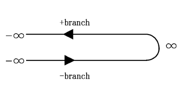
Figure 2.1: time contour which starts and ends at $t=-\infty$ through $t=\infty$

2.1 S-matrix (S-operator)

The Hamiltonian is given by Eq. ( 2.1 ). The time evolution in the interaction representation is expressed in terms of S-matrix by

$${\tilde{\psi}}(t)={S(t,t_{\rm 0})}{\tilde{\psi}}(t_{\rm 0}).$$ (2.2)

S-matrix ${S(t,t_{\rm 0})}$ is defined by

$${S(t,t_{\rm 0})}=e^{i{\cal{H}_{\rm 0}}t/{\hbar}}e^{-i{\cal{H}}(t-t_{0})/{\hbar}}e^{-i{\cal{H}_{\rm 0}}t_{\rm 0}/{\hbar}},$$ (2.3)

and has the following properties:

$$S(t_{\rm 0},t_{\rm 0}) = 1,$$ (2.4)

$$S(t,t_{\rm 0})^{{\dagger}} = S(t_{\rm 0},t),$$ (2.5)

$$S(t_{1},t_{2})S(t_{2},t_{3}) = S(t_{1},t_{3}),$$ (2.6)

$$i{\hbar}{\frac{{\partial}S(t,t_{\rm 0})}{{\partial}t}} = {\tilde{\cal{H}}_{\rm I}}S(t,t_{\rm 0}).$$ (2.7)

Equation ( 2.7 ) can be solved formally by

$${\cal S}(t,t_{\rm 0}) = 1+\sum_{n=1}^{\infty}{\frac{1}{n!}}\left({\frac{-i}{\hbar}}\right)^{n}\int_{t_{\rm 0}}^{t}dt_{1}{\ldots}\int_{t_{\rm 0}}^{t}dt_{n}{\rm T}\left[{\tilde{\cal{H}}_{\rm I}}(t_{1}){\ldots}{\tilde{\cal{H}}_{\rm I}}(t_{n})\right]$$ (2.8)

$$= {\rm T}\left[{\exp}\left\{{\frac{-i}{\hbar}}\int_{t_{\rm 0}}^{t}dt^{{}^{\prime}}{\tilde{\cal{H}}_{\rm I}}(t^{{}^{\prime}})\right\}\right],$$

$${\cal S}(t,t_{\rm 0})^{{\dagger}} = {\cal S}(t_{\rm 0},t)={\tilde{\rm T}}\left[{\exp}\left\{{\frac{i}{\hbar}}\int_{t_{\rm 0}}^{t}dt^{{}^{\prime}}{\tilde{\cal{H}}_{\rm I}}(t^{{}^{\prime}})\right\}\right].$$ (2.9)

Here, the time ordering operator ${\rm T}$ arranges in chronological order and ${\rm\tilde{T}}$ is the anti time ordering operator which arranges in the reverse of chronological order. For the time evolution along the time contour as in Fig. 2.1, S-matrices, Eqs. (2.8) and (2.9) are required for paths on the $(-)$ branch from $t=-{\infty}$ to $t={\infty}$ and on the $(+)$ branch from $t={\infty}$ to $t=-{\infty}$, respectively.

In the same way, S-matrix for imaginary-time perturbative formalism is defined by

$${S_{\tau}({\tau},{\tau}_{\rm 0})}=e^{{\cal{H}_{\rm 0}}{\tau}/{\hbar}}e^{-{\cal{H}}({\tau}-{\tau}_{0})/{\hbar}}e^{-{\cal{H}_{\rm 0}}{\tau}_{\rm 0}/{\hbar}}$$ (2.10)

and is also written by

$${\cal S}_{\tau}({\tau},{\tau}_{\rm 0}) = 1+\sum_{n=1}^{\infty}{\frac{1}{n!}}\left({\frac{-1}{\hbar}}\right)^{n}\int_{{\tau}_{\rm 0}}^{\tau}d{\tau}_{1}{\ldots}\int_{{\tau}_{\rm 0}}^{\tau}d{\tau}_{n}{\rm T_{\tau}}\left[{\tilde{\cal{H}}_{\rm I}}({\tau}_{1}){\ldots}{\tilde{\cal{H}}_{\rm I}}({\tau}_{n})\right]$$ (2.11)

$$= {\rm T}_{\tau}\left[{\exp}\left\{{\frac{-1}{\hbar}}\int_{{\tau}_{\rm 0}}^{\tau}d{\tau}^{{}^{\prime}}{\tilde{\cal{H}}_{\rm I}}({\tau}^{{}^{\prime}})\right\}\right].$$

These are the requisites for the Matsubara imaginary-time perturbative formalism.[14]

2.2 Matsubara Imaginary-Time Perturbative Formalism

For thermal equilibrium, the statistical operator ( density matrix ) is written in Gibbs form for the grand canonical ensemble by

$${\varrho}_{G}={\frac{e^{-{\beta}({\cal H}-{\mu}N)}}{{\rm Tr}e^{-{\beta}({\cal H}-{\mu}N)}}}=e^{{\beta}({\Omega}-{\cal H}+{\mu}N)}.$$ (2.12)

${\beta}=1/k_{B}T.$ By rearranging Eq. ( 2.10 ), we have

$$e^{-{\beta}({\cal H}-{\mu}N)}=e^{-{\beta}({\cal H_{\rm 0}}-{\mu}N)}{S_{\tau}({\beta}{\hbar},0)}.$$ (2.13)

By substitution of Eq. ( 2.13 ) into Eq. ( 2.12 ), the thermal average for equilibrium is obtained by

$${\langle}{\ldots}{\rangle}={\frac{{\rm Tr}[e^{-{\beta}({\cal H}-{\mu}N)}{\ldots}]}{{\rm Tr}[e^{-{\beta}({\cal H}-{\mu}N)}]}}={\frac{{\rm Tr}[e^{-{\beta}({\cal H_{\rm 0}}-{\mu}N)}{S_{\tau}({\beta}{\hbar},0)}{\ldots}]}{{\rm Tr}[e^{-{\beta}({\cal H_{\rm 0}}-{\mu}N)}{S_{\tau}({\beta}{\hbar},0)}].}}$$ (2.14)

By insertion of Eq. ( 2.11 ) in Eq. ( 2.14 ), the perturbative expansion is executed for the Matsubara imaginary-time perturbative formalism[14] using the Bloch and De Dominicis’s theorem[38-41]. The Matsubara Green’s function is defined by

$$G({\tau}){\equiv}-{\langle}{\rm T}_{{\tau}}\hat{d}({\tau})\hat{d}^{{\dagger}}(0){\rangle}.$$ (2.15)

The functions in terms of the Matsubara Green’s function in imaginary-time are converted into those in the Matsubara frequency by the Fourier transformation for the Matsubara Green’s function:

$$G(i{\omega}_{n})=\int_{0}^{{\beta}}d{\tau}e^{i{\omega}_{n}{\tau}}G({\tau}).$$ (2.16)

The Matsubara frequency, ${\omega}_{n}{\equiv}$ $(2n+1){\pi}/{\beta}$ for fermion and ${\omega}_{n}{\equiv}$ $2n{\pi}/{\beta}$ for boson, $(n=0,{\pm}1,$ ${\pm}2,$ ${\pm}3$ ${\ldots}\ \ )$; thereby, the Matsubara Green’s function is periodic.

After that, the analytical continuity is performed. For fermion, when the Taylor expansion for the function ${e^{{\beta}z}+1}$ around poles $z=z^{0}$ on imaginary axis is done, then, ${e^{{\beta}z^{0}}+1}=0$, hence, $z^{0}=(2n+1){\pi}i/{\beta}$, and as approximation, ${e^{{\beta}z}+1}{\approx}{\beta}e^{{\beta}z^{0}}(z-z^{0})$. The residue theorem yields the conversion of sum of the functions in the Matsubara frequency into the contour integral by

$${\frac{1}{\beta}}{\sum_{l}}g(i{\omega}_{l})={\frac{1}{2{\pi}i}}\int_{C}{\frac{g(z)}{e^{{\beta}z}+1.}}$$ (2.17)

It should be noted that the contour $C$ in integral surrounds the poles $z^{0}$ on imaginary axis. After that, for example, when $g(z)=1/(z-{\epsilon}_{d}$), then, the contour integral with contour $C^{\prime}$ enclosing ${\epsilon}_{d}$, a pole on real axis is executed by

$${\frac{1}{2{\pi}i}}\int_{C^{\prime}}{\frac{g(z)}{e^{{\beta}z}+1}}=f({\epsilon}_{d}),$$ (2.18)

where $f({\epsilon}_{d})$ is the Fermi distribution function.

In the same way, in boson case, for poles $z=z^{0}$ on imaginary axis, ${e^{{\beta}z^{0}}-1}=0$, i.e. $z^{0}=2n{\pi}i/{\beta}$, and approximately, ${e^{{\beta}z}-1}{\approx}{\beta}e^{{\beta}z^{0}}(z-z^{0})$, we have

$${\frac{1}{\beta}}{\sum_{l}}g(i{\omega}_{l})=-{\frac{1}{2{\pi}i}}\int_{C}{\frac{g(z)}{e^{{\beta}z}-1.}}$$ (2.19)

Then, by changing the contour integral around poles on imaginary axis into the contour integral parallel with real axis ( e.g. $E{\pm}i{\delta}$ ), we have the functions written in terms of retarded and advanced Green’s functions in energy. For high-order perturbation theory, the analytical continuation is so complicated. As the method of analytical continuation, Éliashberg’s method[42] is known.[4,41]

2.3 Nonequilibrium Perturbative Formalism

2.3.1 Nonequilibrium Real-Time Perturbative Formalism

For nonequilibrium, Equation ( 2.12 ) is not exact. We should note that there are no specific limitations upon the statistical operator. The von Neumann’s statistical operator is expressed independently of whether the states are at thermal equilibrium or nonequilibrium by[35,37]

$${\varrho}_{S}(t)=\sum_{m}|m_{S}(t){\rangle}P_{m}{\langle}m_{S}(t)|$$ (2.20)

in the Schrödinger representation. Here, $P_{m}$ is probability that the system is in state $m$ and $|m_{S}(t){\rangle}$ is the state in the Schrödinger representation. It satisfies the Liouville equation by

$$i{\hbar}{\frac{{\partial}{\varrho}_{S}}{{\partial}t}}=[{\cal{H}},{\varrho}_{S}].$$ (2.21)

The statistical operator in the interaction representation is given by

$${\tilde{\varrho}(t)} = e^{i{\cal{H}_{\rm 0}}t/{\hbar}}{\varrho}_{S}(t)e^{-i{\cal{H}_{\rm 0}}t/{\hbar}},$$ (2.22)

and also obeys the Liouville equation by

$$i{\hbar}{\frac{{\partial}{\tilde{\varrho}}}{{\partial}t}} = [{\tilde{\cal{H}}}_{\rm I},{\tilde{\varrho}}].$$ (2.23)

As a matter of course,

$${\varrho}_{S}(0)={\varrho}_{H}(0)={\tilde{\varrho}(0)},$$ (2.24)

where ${{\varrho}_{H}}(t)$ is statistical operator in the Heisenberg representation. The time evolution is written by means of S-matrix by

$${\tilde{\varrho}}(t)=S(t,t_{\rm 0}){\tilde{\varrho}}(t_{0})S(t_{\rm 0},t).$$ (2.25)

These are the properties of the von Neumann’s statistical operator. Although the von Neumann’s statistical operator Eq. ( 2.20 ) is not an explicit expression, it is still considered to be the same type as Eq. ( 2.14 ) so as to execute the perturbative expansion.

The thermal average for nonequilibrium is drawn in view of the analogy with the imaginary-time perturbative method for the Matsubara Green’s function using S-matrix and the time evolution of the statistical operator, Eq.( 2.25 ). Thus the thermal average of the operators in the Heisenberg representation at $t=0$ can be brought, for example by[3,4,34,37]

$${\langle}{\rm T}A(t)B(t^{{}^{\prime}}){\rangle}$$

$${\equiv} {\rm Tr}\left[{\varrho}_{H}(0){\rm T}A(t)B(t^{{}^{\prime}})\right]$$

$$= {\rm Tr}\left[{\tilde{\varrho}}(-\infty){\cal S}(-\infty,0){\rm T}A(t)B(t^{{}^{\prime}}){\cal S}(0,-\infty)\right]$$

$$= {\rm Tr}\left[{\tilde{\varrho}}(-\infty){\cal S}(-\infty,\infty)\left\{{\rm T}{\cal S}(\infty,-\infty){\tilde{A}(t^{-})}{\tilde{B}(t^{{}^{\prime}-})}\right\}\right]$$

$$= \sum_{n=1}^{\infty}\sum_{m=1}^{\infty}{\frac{1}{n!}}{\frac{1}{m!}}\left({\frac{i}{\hbar}}\right)^{n}\left({\frac{-i}{\hbar}}\right)^{m}\int_{-\infty}^{\infty}dt_{1}{\ldots}\int_{-\infty}^{\infty}dt_{n}\int_{-\infty}^{\infty}dt_{1}^{{}^{\prime}}{\ldots}\int_{-\infty}^{\infty}dt_{m}^{{}^{\prime}}$$

$${\times}{\langle}\left\{{\tilde{\rm T}}{\tilde{\cal{H}}}_{\rm I}(t_{1}^{+}){\ldots}{\tilde{\cal{H}}}_{\rm I}(t_{n}^{+})\right\}\left\{{\rm T}{\tilde{\cal{H}}}_{\rm I}(t_{1}^{{}^{\prime}-}){\ldots}{\tilde{\cal{H}}}_{\rm I}(t_{m}^{{}^{\prime}-}){\tilde{A}(t^{-})}{\tilde{B}(t^{{}^{\prime}-})}\right\}{\rangle}_{av},$$

where ${\langle}{\ldots}{\rangle}_{av}$ means ${\rm Tr}[{\tilde{\varrho}}(-\infty){\ldots}]$. $\tilde{A}$ denotes an arbitrary operator in the interaction representation. Here, $A(t)$$=S(0,t)\tilde{A}(t)S(t,0)$ and ${\varrho}_{H}(0)$$={\tilde{\varrho}}(0)$ $=S(0,-{\infty}){\tilde{\varrho}}$$(-{\infty})S(-{\infty},0)$. In this case, the operators ${\tilde{A}(t^{-})}$ and ${\tilde{B}(t^{{}^{\prime}-})}$ in Eq.( 2.26 ) both are on the $(-)$ branch from $t=-{\infty}$ to $t={\infty}$ of the time contour in Fig. 2.1.

Using the last expression in Eq.( 2.26 ), the real-time perturbative expansion is executed diagrammatically by the help of the Wick’s theorem. On the diagrammatical perturbative expansion, the diagrammatical methods written by Lifshitz and Pitaevskii.[4] are extended.

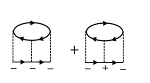
Figure 2.2: The extension of the diagrammatic technique of Lifshitz and Pitaevskii. ${\Sigma}^{--(3)}_{ph}$ brought as the sum over terms going from time $(-)$ to time $(-)$ by way of times $(-)$ and $(+)$.

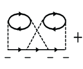
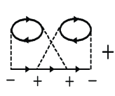
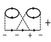
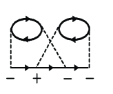
Figure 2.3: ${\Sigma}^{--(4)}_{d}$ brought as the sum of terms passing by way of times, $(-)(-),$ $(+)(+),$ $(-)(+)$ and $(+)(-)$.

There the summation over terms in all times is taken. For example, the third-order self-energy ${\Sigma}^{--(3)}_{ph}$ is brought as the sum over terms going from time $(-)$ to time $(-)$ by way of times $(-)$ and $(+)$ as illustrated in Fig. 2.2. See Fig.2.1 again. It should be noted that the times $(-)$ are on the $(-)$ branch from $t=-{\infty}$ to $t={\infty}$ of the time contour in Fig. 2.1 and the times $(+)$ are on the $(+)$ branch from $t={\infty}$ to $t=-{\infty}$ of the time contour. In addition, for the fourth-order self-energy, ${\Sigma}^{--(4)}_{d},$ the sum of terms passing through times, $(-)(-),$ $(+)(+),$ $(-)(+)$ and $(+)(-)$ is taken, as shown in Fig. 2.3.

2.3.2 Schwinger-Keldysh Formalism

The Dyson’s equation for the Keldysh formalism is given by

$${\bf G} = \ \ {\bf g}\ \ +\ \ {\bf g}\ \ {\bf{\Sigma}}\ \ {\bf G},$$ (2.27)

where

$${\bf G}=\left[\begin{array}[]{ll}G^{--}&G^{<}\\ G^{>}&G^{++}\\ \end{array}\right],\ \ {\bf{\Sigma}}=\left[\begin{array}[]{ll}{\Sigma}^{--}&{\Sigma}^{<}\\ {\Sigma}^{>}&{\Sigma}^{++}\\ \end{array}\right].$$ (2.32)

The nonequilibrium Green’s functions are defined by

$$G^{--}(t_{1},t_{2})\,{\equiv}\,-i{\langle}{\rm T}\hat{d}(t_{1})\hat{d}^{{\dagger}}(t_{2}){\rangle},$$ (2.33)

$$G^{++}(t_{1},t_{2})\,{\equiv}\,-i{\langle}{\rm\tilde{T}}\hat{d}(t_{1})\hat{d}^{{\dagger}}(t_{2}){\rangle},$$ (2.34)

$$G^{>}(t_{1},t_{2})\,{\equiv}\,-i{\langle}\hat{d}(t_{1})\hat{d}^{{\dagger}}(t_{2}){\rangle},$$ (2.35)

$$G^{<}(t_{1},t_{2})\,{\equiv}\,i{\langle}\hat{d}^{{\dagger}}(t_{2})\hat{d}(t_{1}){\rangle}.$$ (2.36)

As shown in Eq. ( 2.26 ), the operators in Eq. ( 2.28 ) both are on the $(-)$ branch from $t=-{\infty}$ to $t={\infty}$ of the time contour in Fig. 2.1. In the same way, those in Eq. ( 2.29 ) both are on the $(+)$ branch from $t={\infty}$ to $t=-{\infty}$ of the time contour, and those in Eq. ( 2.30 ) are on the $(+)$ branch and on the $(-)$ branch, respectively. In Eq. ( 2.31 ), they are on the $(-)$ branch and on the $(+)$ branch, respectively.

Additionally, retarded and advanced Green’s functions are defined by

$$G^{r}(t_{1},t_{2})\,{\equiv}\,-i{\theta}(t_{1}-t_{2}){\langle}\{\hat{d}(t_{1}),\hat{d}^{{\dagger}}(t_{2})\}{\rangle},$$ (2.37)

$$G^{a}(t_{1},t_{2})\,{\equiv}\,i{\theta}(t_{2}-t_{1}){\langle}\{\hat{d}(t_{1}),\hat{d}^{{\dagger}}(t_{2})\}{\rangle}.$$ (2.38)

Here, the curly brackets signifies anticommutator. The Dyson’s equations for retarded and advanced Green’s functions are given by

$$G^{r} = \ \ g^{r}\ \ +\ \ g^{r}\ \ {\Sigma}^{r}\ \ G^{r},$$ (2.39)

$$G^{a} = \ \ g^{a}\ \ +\ \ g^{a}\ \ {\Sigma}^{a}\ \ G^{a}.$$ (2.40)

As the necessity to Eqs. ( 2.34 ) and ( 2.35 ), the self-energies ${\Sigma}^{r}$ and ${\Sigma}^{a}$ must be retarded and advanced functions in time, respectively.

In accordance with the ordinary procedure of nonequilibrium perturbative formalism,[3,4, 34,35,37] for the Dyson’s equation for the Keldysh formalism, Eq. ( 2.27 ), the transformation is carried out: by use of

$${\bf L}=[{\bf L^{{\dagger}}}]^{-1}={\frac{1}{\sqrt{2}}}\left[\begin{array}[]{ll}1&-1\\ 1&1\\ \end{array}\right],$$ (2.43)

$${\bf{G}}=\left[\begin{array}[]{ll}{G}^{--}&{G}^{<}\\ {G}^{>}&{G}^{++}\\ \end{array}\right]\ \ {\longrightarrow}\ \ {\bf L}{\bf{G}}{\bf L^{{\dagger}}}=\left[\begin{array}[]{ll}{0}&{G}^{a}\\ {G}^{r}&{G}^{K}\\ \end{array}\right],$$ (2.48)

and

$${\bf{\Sigma}}=\left[\begin{array}[]{ll}{\Sigma}^{--}&{\Sigma}^{<}\\ {\Sigma}^{>}&{\Sigma}^{++}\\ \end{array}\right]\ \ {\longrightarrow}\ \ {\bf L}{\bf{\Sigma}}{\bf L^{{\dagger}}}=\left[\begin{array}[]{ll}{\Omega}&{\Sigma}^{r}\\ {\Sigma}^{a}&0\\ \end{array}\right].$$ (2.53)

From the definition of Green’s functions,

$${G}^{r} = {G}^{--}-{G}^{<}={G}^{>}-{G}^{++},$$

$${G}^{a} = {G}^{--}-{G}^{>}={G}^{<}-{G}^{++},$$

in other words,

$${G}^{r}(t) = [{G}^{>}(t)-{G}^{<}(t)]{\theta}(t),$$

$${G}^{a}(t) = [{G}^{<}(t)-{G}^{>}(t)]{\theta}(-t).$$

${G}^{K}$ is called the Keldysh Green’s function. For the self-energies part, the following relationship is required:

$${\Sigma}^{r}(t) = {\Sigma}^{--}(t)+{\Sigma}^{<}(t)=-{\Sigma}^{++}(t)-{\Sigma}^{>}(t),$$ (2.54)

$${\Sigma}^{a}(t) = {\Sigma}^{--}(t)+{\Sigma}^{>}(t)=-{\Sigma}^{++}(t)-{\Sigma}^{<}(t),$$ (2.55)

$${\Omega}(t) = {\Sigma}^{--}(t)+{\Sigma}^{++}(t)=-{\Sigma}^{<}(t)-{\Sigma}^{>}(t).$$ (2.56)

The above is known in general. Here, it is uncertain whether or not the requirements of self-energies as functions in time are fulfilled. It is because the definition of the self-energies in matrix form is not given, as mentioned earlier.

The solution is given from the present work.[43] That is explained as follows: in the right-hand sides of Eqs. ( 2.36 ), ( 2.37 ) and ( 2.38 ), the functions, ${\Sigma}^{--}(t),$ ${\Sigma}^{<}(t),$ ${\Sigma}^{++}(t)$ and ${\Sigma}^{>}(t)$ are deduced from perturbative expansion with the Wick’s theorem. At this time, the directions in time are not defined in the functions ${\Sigma}^{--}(t),$ ${\Sigma}^{<}(t),$ ${\Sigma}^{++}(t)$ and ${\Sigma}^{>}(t)$. This is due to the following functions in dependence upon time:

$$g^{--}(t)={\theta}(t)g^{>}(t)+{\theta}(-t)g^{<}(t),$$ (2.57)

$$g^{++}(t)={\theta}(t)g^{<}(t)+{\theta}(-t)g^{>}(t).$$ (2.58)

For this reason, for the right-hand sides of Eqs. ( 2.36 ), ( 2.37 ) and ( 2.38 ), the directions in time must necessarily be taken into consideration.

As the main point, the terms in the right-hand sides are taken for sum of retarded and advanced terms:

$${\Sigma}^{r}(t) = [{\Sigma}^{--}(t)+{\Sigma}^{<}(t)]{\theta}(t)+[{\Sigma}^{--}(t)+{\Sigma}^{<}(t)]{\theta}(-t)$$ (2.59)

$$= -[{\Sigma}^{++}(t)+{\Sigma}^{>}(t)]{\theta}(t)-[{\Sigma}^{++}(t)+{\Sigma}^{>}(t)]{\theta}(-t),$$

$${\Sigma}^{a}(t) = [{\Sigma}^{--}(t)+{\Sigma}^{>}(t)]{\theta}(t)+[{\Sigma}^{--}(t)+{\Sigma}^{>}(t)]{\theta}(-t)$$ (2.60)

$$= -[{\Sigma}^{++}(t)+{\Sigma}^{<}(t)]{\theta}(t)-[{\Sigma}^{++}(t)+{\Sigma}^{<}(t)]{\theta}(-t),$$

$${\Omega}(t) = [{\Sigma}^{--}(t)+{\Sigma}^{++}(t)]{\theta}(t)+[{\Sigma}^{--}(t)+{\Sigma}^{++}(t)]{\theta}(-t)$$ (2.61)

$$= -[{\Sigma}^{<}(t)+{\Sigma}^{>}(t)]{\theta}(t)-[{\Sigma}^{<}(t)+{\Sigma}^{>}(t)]{\theta}(-t).$$

For self-energy functions derived by the present perturbative expansion via the Wick’s theorem, the following relations are found:

$${\Sigma}^{--}(t){\theta}(t)=-{\Sigma}^{>}(t){\theta}(t),$$ (2.62)

$${\Sigma}^{++}(t){\theta}(t)=-{\Sigma}^{<}(t){\theta}(t),$$ (2.63)

$${\Sigma}^{--}(t){\theta}(-t)=-{\Sigma}^{<}(t){\theta}(-t),$$ (2.64)

$${\Sigma}^{++}(t){\theta}(-t)=-{\Sigma}^{>}(t){\theta}(-t);$$ (2.65)

these relations have never been known in general. When these are substituted into Eqs. ( 2.41 ), ( 2.42 ) and ( 2.43 ), then, the advanced term of Eq. ( 2.41 ) and the retarded term of Eq. ( 2.42 ) are canceled:

$$[{\Sigma}^{--}(t)+{\Sigma}^{<}(t)]{\theta}(-t)=-[{\Sigma}^{++}(t)+{\Sigma}^{>}(t)]{\theta}(-t)=0,$$ (2.66)

$$[{\Sigma}^{--}(t)+{\Sigma}^{>}(t)]{\theta}(t)=-[{\Sigma}^{++}(t)+{\Sigma}^{<}(t)]{\theta}(t)=0,$$ (2.67)

so that Equations ( 2.41 ) and ( 2.42 ) reduce to

$${\Sigma}^{r}(t) = [{\Sigma}^{--}(t)+{\Sigma}^{<}(t)]{\theta}(t)=-[{\Sigma}^{++}(t)+{\Sigma}^{>}(t)]{\theta}(t),$$ (2.68)

$${\Sigma}^{a}(t) = [{\Sigma}^{--}(t)+{\Sigma}^{>}(t)]{\theta}(-t)=-[{\Sigma}^{++}(t)+{\Sigma}^{<}(t)]{\theta}(-t).$$ (2.69)

The retarded and advanced self-energies are acquired as retarded and advanced functions in time, respectively; they are the requirements. In addition, Equation ( 2.43 ) is certainly reproduced.

Then, it leads to

$${\Sigma}^{r}(t) = [{\Sigma}^{<}(t)-{\Sigma}^{>}(t)]{\theta}(t),$$ (2.70)

$${\Sigma}^{a}(t) = [{\Sigma}^{>}(t)-{\Sigma}^{<}(t)]{\theta}(-t);$$ (2.71)

they consist with the expressions in the review by Rammer and Smith.[44] The formalism in the review of Rammer and Smith is different from the nonequilibrium perturbative expansion, so that the present method is confirmed to connect with the other formalism. By performing the Fourier transformation for Eqs. ( 2.52 ) and ( 2.53 ), we have

$${\Sigma}^{r}(E)-{\Sigma}^{a}(E)={\Sigma}^{<}(E)-{\Sigma}^{>}(E);$$ (2.72)

it proves that the relation stands. Since Equation ( 2.54 ) is widely known, Equations ( 2.52 ) and ( 2.53 ) should generally hold as functions in time.

Besides,

$$G^{<} = (1+G^{r}{\Sigma}^{r})g^{<}(1+G^{a}{\Sigma}^{a})-G^{r}{\Sigma}^{<}G^{a},$$ (2.73)

$$G^{>} = (1+G^{r}{\Sigma}^{r})g^{>}(1+G^{a}{\Sigma}^{a})-G^{r}{\Sigma}^{>}G^{a}$$ (2.74)

and

$$G^{K} = (1+G^{r}{\Sigma}^{r})g^{K}(1+G^{a}{\Sigma}^{a})+G^{r}{\Omega}G^{a}$$ (2.75)

still work.

As mentioned above, the present solution is in accordance with the generally known relations. It indicates that the present solution has validity.

Chapter 3 Expressions of Self-Energy for Anderson model

3.1 Anderson model

We consider equilibrium and nonequilibrium stationary states. Nonequilibrium state is caused by finite bias voltage, that is, the difference of chemical potentials; after bias voltage was turned on, long time has passed enough to reach stationary states. Since the states are stationary, the Hamiltonian has no time dependence. The system is described by the Anderson model linking to leads. The impurity ( the quantum dot ) with on-site energy $E_{0}$ and the Coulomb interaction $U$ is connected to the left and right leads by the mixing matrix elements, $v_{L}$ and $v_{R}$. The system is illustrated below.

U=0

Left Lead

    $v_{L}$      U${\neq}$0 Quantum Dot     $v_{R}$      U=0 Right Lead

The Anderson Hamiltonian is given by

$${\cal H}= E_{0}\sum_{\sigma}\hat{n}_{d{\sigma}}+{\mu}_{L}\sum_{\sigma}\hat{n}_{L{\sigma}}+{\mu}_{R}\sum_{\sigma}\hat{n}_{R{\sigma}}+U\bigl{(}\hat{n}_{d\uparrow}-{\langle}\hat{n}_{d\uparrow}{\rangle}\bigr{)}\bigl{(}\hat{n}_{d\downarrow}-{\langle}\hat{n}_{d\downarrow}{\rangle}\bigr{)}$$ (3.1)

$$-\sum_{{\sigma}}v_{L}\bigl{(}\hat{d}_{{\sigma}}^{{\dagger}}\hat{c}_{L{\sigma}}+{\rm H.c.}\bigr{)}-\sum_{{\sigma}}v_{R}\bigl{(}\hat{d}_{{\sigma}}^{{\dagger}}\hat{c}_{R{\sigma}}+{\rm H.c.}\bigr{)}.$$

$\hat{d}^{{\dagger}}$ ($\hat{d}$) is creation (annihilation) operator for electron on the impurity, and $\hat{c}_{L}^{{\dagger}}$ and $\hat{c}_{R}^{{\dagger}}$ ($\hat{c}_{L}$ and $\hat{c}_{R}$) are creation (annihilation) operators in the left and right leads, respectively. ${\sigma}$ is index for spin. The chemical potentials in the isolated left and right leads are ${\mu}_{L}$ and ${\mu}_{R},$ respectively. The applied voltage is, therefore defined by $eV\,{\equiv}\,{\mu}_{L}-{\mu}_{R}$.

We consider that the band-width of left and right leads is large infinitely, so that the coupling functions, ${\Gamma}_{L}$ and ${\Gamma}_{R}$ can be taken to be independent of energy, $E$. On-site energy $E_{0}$ is set being canceled with the Hartree term, i.e. the first-order contribution to self-energy for electron correlation, as mentioned later.

Accordingly, the Fourier components of the noninteracting ( unperturbed ) Green’s functions reduce to

$$g^{r}(E) = {\frac{1}{E+i{\Gamma},}}$$ (3.2)

$$g^{a}(E) = {\frac{1}{E-i{\Gamma}.}}$$ (3.3)

where ${\Gamma}=({\Gamma}_{L}+{\Gamma}_{R})/2$. Hence, the inverse Fourier components can be written by

$$g^{r}(t)=-i{\theta}(t)e^{-{\Gamma}t},$$ (3.4)

$$g^{a}(t)=i{\theta}(-t)e^{{\Gamma}t}.$$ (3.5)

In addition, by solving the Dyson’s equation Eq. ( 2.27 ), we have

$$g^{<}(E)=g^{r}(E)\,\bigl{[}\,if_{L}(E){\Gamma}_{L}+if_{R}(E){\Gamma}_{R}\,\bigr{]}\,g^{a}(E),$$ (3.6)

$$g^{>}(E)=g^{r}(E)\,\bigl{[}\,i(f_{L}(E)-1){\Gamma}_{L}+i(f_{R}(E)-1){\Gamma}_{R}\,\bigr{]}\,g^{a}(E).$$ (3.7)

$f_{L}$ and $f_{R}$ are the Fermi distribution functions in the isolated left and right leads, respectively. By Eqs. ( 3.6 ) and ( 3.7 ), the nonequilibrium state is introduced effectively as the superposition of the left and right leads. In this case, the effective Fermi distribution function can be expressed by[8]

$$f_{\rm eff}(E)={\frac{f_{L}(E){\Gamma}_{L}+f_{R}(E){\Gamma}_{R}}{{\Gamma}_{L}+{\Gamma}_{R}}}.$$ (3.8)

This effective Fermi distribution function is reasonable because it is considered that leads have the continuous energy states and the two chemical potentials are not two localized states.

3.2 Self-Energy

The expressions for self-energies of the Coulomb interaction of the Anderson model are formulated by the method of the nonequilibrium perturbation theory based on the adiabatic theorem, explained in Chapter 2. Practically, the perturbative expansion is done with respect to the Coulomb interaction term of Eq. ( 3.1 ) using the last expression of Eq. ( 2.26 ) in view of the Dyson’s equation Eq. ( 2.27 ) and each diagram. In ${\Sigma}^{--}(t),$ ${\Sigma}^{<}(t),$ ${\Sigma}^{++}(t)$ and ${\Sigma}^{>}(t)$ obtained by the present solution, Equations (2.44)-(2.47) are satisfied. Every formulated ${\Sigma}^{r}(E)$ and ${\Sigma}^{a}(E)$ are in the relation of the complex conjugate each other.

3.2.1 First-Order Contribution

For the Anderson model, the first-order contribution, the Hartree term can be written by

$${\Sigma}^{r(1)}(E)={\Sigma}^{a(1)}(E) = U{\langle}n{\rangle}=U\int{\frac{dE}{2{\pi}i}}G^{<}(E),$$ (3.9)

where ${\langle}n{\rangle}$ is charge density.

3.2.2 Second-Order Contribution

The second-order self-energies are expressed by

$${\Sigma}^{r(2)}(E)=U^{2}\int^{\infty}_{0}{dt_{1}}e^{iEt_{1}}\left[\begin{array}[]{llll}\ \ g^{>}(t_{1})g^{>}(t_{1})g^{<}(-t_{1})\\ -g^{<}(t_{1})g^{<}(t_{1})g^{>}(-t_{1})\end{array}\right]$$ (3.12)

$$=U^{2}\int^{\infty}_{0}{dt_{1}}e^{iEt_{1}}\left[\begin{array}[]{llll}\ \ g^{\pm}(t_{1})g^{>}(t_{1})g^{<}(-t_{1})\\ +g^{<}(t_{1})g^{\pm}(t_{1})g^{>}(-t_{1})\\ +g^{<}(t_{1})g^{>}(t_{1})g^{\pm}(-t_{1})\end{array}\right],$$ (3.16)

$${\Sigma}^{a(2)}(E)=U^{2}\int^{0}_{-\infty}{dt_{1}}e^{iEt_{1}}\left[\begin{array}[]{llll}\ \ g^{<}(t_{1})g^{<}(t_{1})g^{>}(-t_{1})\\ -g^{>}(t_{1})g^{>}(t_{1})g^{<}(-t_{1})\end{array}\right]$$ (3.19)

$$=U^{2}\int^{0}_{-\infty}{dt_{1}}e^{iEt_{1}}\left[\begin{array}[]{llll}\ \ g^{\pm}(t_{1})g^{>}(t_{1})g^{<}(-t_{1})\\ +g^{<}(t_{1})g^{\pm}(t_{1})g^{>}(-t_{1})\\ +g^{<}(t_{1})g^{>}(t_{1})g^{\pm}(-t_{1})\end{array}\right].$$ (3.23)

Here $g^{\pm}(t)=g^{r}(t)+g^{a}(t),$ that is, $g^{+}(t)=g^{r}(t)=-i{\theta}(t)e^{-{\Gamma}t}$ for $t{\geq}0$ and $g^{-}(t)=g^{a}(t)=i{\theta}(-t)e^{{\Gamma}t}$ for $t<0$. Additionally, $g^{<}(t)$ and $g^{>}(t)$ are the inverse Fourier components of Eqs. ( 3.6 ) and ( 3.7 ). Figure 3.1 shows the diagram for the second-order self-energy. These expressions for equilibrium agree exactly with those deduced from the Matsubara imaginary-time perturbative expansion for equilibrium and analytical continuity by Zlatić et al.[45]. As shown numerically later, the second-order contribution coincide with those brought out by Hershfield et al.[8].

In the symmetric equilibrium case, the asymptotic behavior at low energy is expressed by

$${\Sigma}^{r(2)}(E){\simeq}-{\Gamma}\left(3-{\frac{{\pi}^{2}}{4}}\right)\left(\frac{U}{{\pi}{\Gamma}}\right)^{2}\frac{E}{\Gamma}-i\frac{\Gamma}{2}\left(\frac{U}{{\pi}{\Gamma}}\right)^{2}\left(\frac{E}{\Gamma}\right)^{2},$$ (3.24)

the exact results based on the Bethe ansatz method.[46,47]

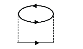
Figure 3.1: The second-order self-energy

3.2.3 Third-Order and Fourth-Order Contributions

There are two kinds of the third-order contributions as illustrated in Fig. 3.2.

$${\Sigma}^{r(3)}_{pp}(E) = U^{3}\int^{\infty}_{0}{dt_{1}}\int^{\infty}_{-\infty}{dt_{2}}e^{iEt_{1}}\,\left[\begin{array}[]{llll}g^{<}(-t_{1})g^{>}(t_{1}-t_{2})g^{>}(t_{1}-t_{2})\\ -g^{>}(-t_{1})g^{<}(t_{1}-t_{2})g^{<}(t_{1}-t_{2})\\ \end{array}\right]$$ (3.27)

$${\times}\left[\begin{array}[]{llll}g^{\pm}(t_{2})g^{>}(t_{2})+g^{<}(t_{2})g^{\pm}(t_{2})\end{array}\right],$$

$${\Sigma}^{a(3)}_{pp}(E) = U^{3}\int^{0}_{-\infty}{dt_{1}}\int^{\infty}_{-\infty}{dt_{2}}e^{iEt_{1}}\,\left[\begin{array}[]{llll}g^{>}(-t_{1})g^{<}(t_{1}-t_{2})g^{<}(t_{1}-t_{2})\\ -g^{<}(-t_{1})g^{>}(t_{1}-t_{2})g^{>}(t_{1}-t_{2})\\ \end{array}\right]$$ (3.30)

$${\times}\left[\begin{array}[]{llll}g^{\pm}(t_{2})g^{>}(t_{2})+g^{<}(t_{2})g^{\pm}(t_{2})\end{array}\right].$$

$${\Sigma}^{r(3)}_{ph}(E) = U^{3}\int^{\infty}_{0}{dt_{1}}\int^{\infty}_{-\infty}{dt_{2}}e^{iEt_{1}}\,\left[\begin{array}[]{llll}g^{>}(t_{1})g^{>}(t_{1}-t_{2})g^{<}(t_{2}-t_{1})\\ -g^{<}(t_{1})g^{<}(t_{1}-t_{2})g^{>}(t_{2}-t_{1})\\ \end{array}\right]$$ (3.33)

$${\times}\left[\begin{array}[]{llll}g^{\pm}(t_{2})g^{<}(-t_{2})+g^{<}(t_{2})g^{\pm}(-t_{2})\end{array}\right],$$

$${\Sigma}^{a(3)}_{ph}(E) = U^{3}\int^{0}_{-\infty}{dt_{1}}\int^{\infty}_{-\infty}{dt_{2}}e^{iEt_{1}}\,\left[\begin{array}[]{llll}g^{<}(t_{1})g^{<}(t_{1}-t_{2})g^{>}(t_{2}-t_{1})\\ -g^{>}(t_{1})g^{>}(t_{1}-t_{2})g^{<}(t_{2}-t_{1})\\ \end{array}\right]$$ (3.36)

$${\times}\left[\begin{array}[]{llll}g^{\pm}(t_{2})g^{<}(-t_{2})+g^{<}(t_{2})g^{\pm}(-t_{2})\end{array}\right].$$

Equations (3.13)-(3.16) for equilibrium state agree exactly with those derived from the Matsubara imaginary-time perturbative expansion for equilibrium and analytical continuity by Zlatić et al.[45]. As mentioned later, it is numerically confirmed that the third-order contribution is canceled for the symmetric Anderson model; this is compatible with both the results deduced from the Yamada-Yosida theory[30,47,48] and gained on the basis of the Bethe ansatz method[46].

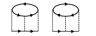
Figure 3.2: Two kinds of the third-order self-energies: ${\Sigma}^{(3)}_{pp}$(Left) and ${\Sigma}^{(3)}_{ph}$

Furthermore, the fourth-order contribution to the self-energy is formulated. ( See Appendix. ) The twelve terms for the proper fourth-order self-energy can be divided into four groups, each of which comprises three terms, corresponding diagrams Fig. 3.3 (a)-(c), (d)-(f), (g)-(i) and (j)-(l), respectively.

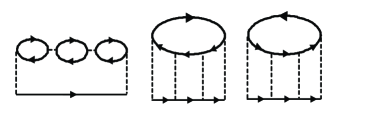
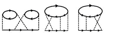
Figure 3.3: The twelve terms for the proper fourth-order self-energy divided into four groups: (a)-(c), (d)-(f), (g)-(i), and (j)-(l).

For symmetric Anderson model at equilibrium, the asymptotic behavior at low energy is approximately in agreement with those based on the Bethe ansatz method[46]:

$${\Sigma}^{r(4)}(E){\simeq}-{\Gamma}\left(105-{\frac{45{\pi}^{2}}{4}}+{\frac{{\pi}^{4}}{16}}\right)\left(\frac{U}{{\pi}{\Gamma}}\right)^{4}\frac{E}{\Gamma}-i\frac{\Gamma}{2}\left(30-3{\pi}^{2}\right)\left(\frac{U}{{\pi}{\Gamma}}\right)^{4}\left(\frac{E}{\Gamma}\right)^{2}.$$

The fourth-order contribution has not been clarified well. In particular, the behavior for nonequilibrium state has almost been unknown. In Chapter 4, the numerical results are shown and discussed.

Chapter 4 Numerical Results and Discussion

4.1 Self-Energy

The third-order terms, Eqs. ( 3.13 )-( 3.16 ) are canceled under electron-hole symmetry not only at equilibrium but also at nonequilibrium:

$${\Sigma}^{r(3)}_{ph}(E) = -{\Sigma}^{r(3)}_{pp}(E),$$

$${\Sigma}^{a(3)}_{ph}(E) = -{\Sigma}^{a(3)}_{pp}(E).$$

As a consequence, the third-order contribution to self-energy vanishes in the symmetric case. It is consistent with the results of Refs. [30, 47, 48] based on the Yamada-Yosida theory that all odd-order contributions except the Hartree term become null for equilibrium in the symmetric single-impurity Anderson model; probably, it is just the same with nonequilibrium state. On the other hand, the third-order terms contribute to the asymmetric system where electron-hole symmetry breaks and furthermore, the third-order terms for spin-up and for spin-down contribute respectively when the spin degeneracy is lifted for example, by magnetic field.

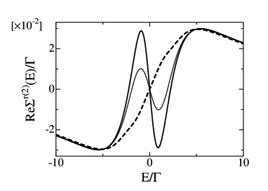
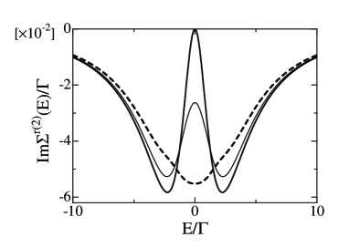
Figure 4.1: The second-order self-energy for the symmetric Anderson model at $U/{\Gamma}=1.0$ and zero temperature. Left:real part and Right:imaginary part at equilibrium ( solid line ), $eV/{\Gamma}=1.0$ ( thin solid line ) and $eV/{\Gamma}=2.0$ ( dashed line ).

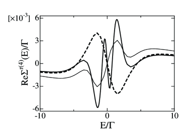
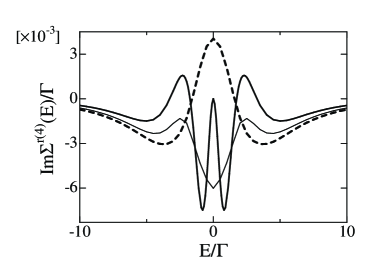
Figure 4.2: The fourth-order self-energy for the symmetric Anderson model at $U/{\Gamma}=1.0$ and zero temperature. Left:real part and Right:imaginary part at equilibrium ( solid line ), $eV/{\Gamma}=1.0$ ( thin solid line ), and $eV/{\Gamma}=2.0$ ( dashed line ). The fourth-order contribution for equilibrium has the same but narrow curves at low energy with those of the second-order contribution.

For the fourth-order contribution, three terms which constitute each of four groups contribute equivalently under electron-hole symmetry. Moreover, to the asymmetric system, the terms brought by the diagrams of Fig. 3.3(a) and (b) contribute equivalently and the terms by the diagrams of Fig. 3.3(j) and (k) make equivalent contribution, and the rest, the eight terms contribute respectively. Further, the twenty-four terms for spin-up and spin-down take effect severally in the presence of magnetic field.

The second-order and the fourth-order contributions to self-energy for zero temperature symmetric Anderson model are plotted in Fig. 4.1 and in Fig. 4.2, respectively. Equation ( 3.12 ) represents the curves around $E=0$ denoted by solid line in Fig. 4.1, and Equation ( 3.17 ) represents approximately those shown in Fig. 4.2. The curves of the second-order self-energy shown in Fig. 4.1 are identical with those of expressions derived by Hershfield et al.[8]. In comparison of Fig. 4.2 with Fig. 4.1, it is found that the fourth-order contribution for equilibrium has the same but narrow curves at low energy with those of the second-order contribution. In addition, the broad curves are attached at high energy for the fourth-order self-energy. ( The higher contribution is, the more should the curves oscillate as a function of energy. ) When the voltage, $eV/{\Gamma}$ exceeds ${\sim}2.0,$ the behavior of curves of self-energy changes distinctly and comes to present a striking contrast to that for the second-order contribution. Especially, the curve for the imaginary part of the fourth-order contribution rises up with maximum at $E=0$. On the other hand, for the second-order contribution, a valley appears with minimum at energy of zero$-$it is quite the contrary. Moreover, from these results, it is expected that the sixth-order contribution to imaginary part of self-energy has minimum at $E=0$. By reason of these, the perturbative expansion is hard to converge for $eV/{\Gamma}>{\sim}2.0,$ as mentioned later.

4.2 Current Conservation

In this section, the problem on the current conservation is described below. In Ref. [8], it is shown that the continuity of current entering and leaving the impurity stands exactly at any strength of $U$ within the approximation up to the second-order for the symmetric single-impurity Anderson model. In comparison of Fig. 4.2 with Fig. 4.1, it is found that curves of fourth-order self-energy have the symmetry similar to those of the second-order. From this, it is anticipated that the current conservation are kept perfectly with approximation up to the fourth-order in the single-impurity system where electron-hole symmetry holds. The continuity of current can be maintained perfectly in single-impurity system as far as electron-hole symmetry stands. On the other hand, current comes to fail to be conserved with increasing $U$ in asymmetric single-impurity case and in two-impurity case.

4.3 Spectral Function

4.3.1 For Second-Order Self-Energy

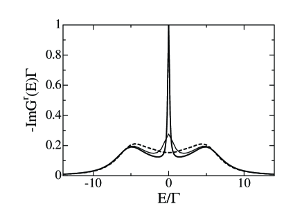
Figure 4.3: The spectral function with the second-order self-energy at $U/{\Gamma}=10.0$ for the symmetric Anderson model at equilibrium ( solid line ), $eV/{\Gamma}=1.0$ ( thin solid line ) and $eV/{\Gamma}=2.0$ ( dashed line ).

The spectral function with the second-order self-energy is widely known. [8][47] It is plotted for $U/{\Gamma}=10.0$ and zero temperature in Fig. 4.3. For equilibrium, the Kondo peak at energy of zero is very sharp and the two-side broad peaks appear at $E{\simeq}$ ${\pm}U/2$. The curve for $eV=0$ is identical with that shown in Ref. [47]. As $eV$ becomes higher than the Kondo temperatures, $k_{B}T_{K}$[49], the Kondo peak becomes lower and is lost finally, while the two-side broad peaks rise at $E{\simeq}$ ${\pm}U/2$.[8]

4.3.2 For Self-Energy up to Fourth-Order for Equilibrium

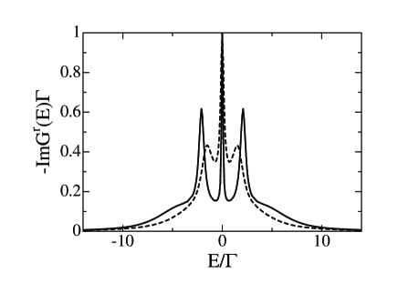
Figure 4.4: The spectral function with self-energy up to the fourth-order at equilibrium for the symmetric Anderson model at $U/{\Gamma}=3.5$ ( dashed line ) and $U/{\Gamma}=5.0$ ( solid line ).

Figure 4.4 shows the spectral function with the self-energy up to the fourth-order for equilibrium and zero temperature. With strengthening $U,$ two-side narrow peaks come to occur in the vicinity of $E=$ ${\pm}U/2$ in addition to the Kondo peak. At $U$ large enough, the Kondo peak becomes very acute and two-side narrow peaks rise higher and sharpen; the energy levels for the atomic limit are produced distinctly. As before, the fourth-order self-energy has the same but narrow curves as functions of energy with those of the second-order and those curves make the peaks at $E=$ ${\pm}U/2$.

For the present approximation up to the fourth-order, the Kondo peak at $E=0$ reaches the unitarity limit and the charge, ${\langle}n{\rangle}$ corresponds to $1/2,$ that is, the Friedel sum rule is correctly satisfied[50]:

$${\rho}(E_{f})={\sin}^{2}({\pi}{\langle}n{\rangle})/{\pi}{\Gamma}.$$ (4.1)

where ${\rho}(E_{f})$ is the local density of states at the Fermi energy.

Here, the discussions should be made on the ranges of $U$ in which the present approximation up to the fourth-order stands. From the results, it is found that the approximation within the fourth-order holds up to $U/{\Gamma}$ ${\sim}5.0$ and is beyond the validity for $U/{\Gamma}$$>{\sim}6.0$. In such a case, the higher-order terms are required.

4.3.3 For Self-Energy up to Fourth-Order for Nonequilibrium

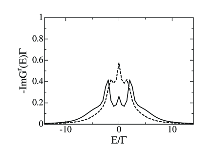
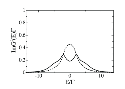
Figure 4.5: The spectral functions with self-energy up to the fourth-order at $eV/{\Gamma}=0.5$ ( Left ) and $eV/{\Gamma}=1.0$ ( Right ) for the symmetric Anderson model. $U/{\Gamma}=3.5$ ( dashed line ) and $U/{\Gamma}=5.0$ ( solid line ).

Next, the results for nonequilibrium and zero temperature are shown. The expression for the Friedel sum rule, Eq. ( 4.1 ) does not stand for nonequilibrium, since the charge cannot be expressed with respect to the local density of states. All the same, the Kondo peak reaches the unitarity limit and ${\langle}n{\rangle}=1/2$ in the symmetric and noninteracting case.

The spectral functions with the self-energy up to the fourth-order are plotted for $eV/{\Gamma}=0.5$ and $eV/{\Gamma}=1.0$ in Fig. 4.5, respectively. The Kondo temperatures lessen with the rise of $U$, as in general known. Approximately[49],

$$k_{B}T_{K}{\sim}\sqrt{\frac{U{\Gamma}}{2}}e^{-{\pi}U/8{\Gamma}+{\pi}{\Gamma}/2U},$$ (4.2)

As the estimation from Eq. ( 4.2 ), $k_{B}T_{K}/$${\Gamma}$ ${\sim}$$0.5$ for $U/$${\Gamma}$ $=3.5$ and $k_{B}T_{K}/$${\Gamma}$ ${\sim}$$0.3$ for $U/$${\Gamma}$$=5.0$. When $U$ is strengthened and $eV$ exceeds $k_{B}T_{K}$, the Kondo peak for $eV/{\Gamma}=0.5$ falls in and instead, the two-side narrow peaks remain to sharpen in the vicinity of $E=$ ${\pm}U/2$. For $eV/{\Gamma}=1.0,$ the Kondo peak becomes broad and disappears for $U$ large enough. The two-side peaks is generated small in the vicinity of $E=$ ${\pm}U/2$. The Kondo resonance is quite broken for bias voltage exceeding the Kondo temperatures; this accords with the experimental results of two terminal systems that the Kondo effect is suppressed when source-drain bias voltage is comparable to or exceeds the Kondo temperatures, $eV{\geq}k_{B}T_{K}$.[32,33]

For $eV/{\Gamma}>{\sim}2.0,$ the Kondo peak does not lower even when $eV$ is much larger than $k_{B}T_{K}$. The perturbative expansion is hard to converge on account of the imaginary part of the self-energy for $eV/{\Gamma}>{\sim}2.0,$ as described before; thereby, the higher-order contribution is probably needed for high voltage. Additionally, for high bias voltage, the picture of the nonequilibrium state represented as the superposition of the two leads is hard to stand.

We have to consider not only the Kondo effect but also the nonequilibrium state caused by bias voltage. In the present work, nonequilibrium state is represented as the superposition of the two leads. As is known, this works well as expression of nonequilibrium state. In this connection, the Khlus-Lesovik formula[11], the expression for current noise is drawn from the present picture[10] and is quantitatively consistent with experiments in ballistic systems. Thereby, the present picture can be valid as description of nonequilibrium state. The effective Fermi distribution function, Eq. ( 3.8 ) is found qualitatively similar to that for finite temperatures $f_{T}(E)$. For example, for finite temperatures $T{\neq}0$,

$$f_{T}(E)[1-f_{T}(E)]{\neq}0,$$

it is indicated that there are thermal charge fluctuations. In case of the effective Fermi distribution function,

$$f_{\rm eff}(E)[1-f_{\rm eff}(E)]{\neq}0$$

for finite voltage $eV{\neq}0$. From this analogy in the Fermi distribution function, it is inferred that there are nonequilibrium fluctuations similar to thermal fluctuations. Because of the effective Fermi distribution function, not only for the second-order but also for the fourth-order, the Kondo resonance is destroyed, qualitatively the same as for finite temperatures,[51] as is observed in experiments of two terminal systems. This is because the energy states in the leads are not discrete but continuous. The present results indicate that the Kondo resonance splitting due to bias voltage does not take place for simple two terminal systems.

Over a decade, it has been expected that the Kondo resonance splits by bias voltage and work as two channels for two channel Kondo effect, so that many endeavours have been made to seek the Kondo peak splitting. Recently, it has been reported that the two channel Kondo effect is observed in quantum dots system.[52] On the experiment, it is not observed for two infinite leads system which has continuous energy state. That occurs for the system that a large dot with closely discrete energy levels is added to two infinite leads system where a large dot works as finite size reservoir and two infinite leads system acts as an infinite reservoir. The observed differential conductance depends on bias voltage and temperatures; this characteristic shows the functions of bias voltage and temperatures for two channel Kondo effect, derived by the theoretical work with conformal field theory.[20-22]

Chapter 5 Summary

In the present work, the solution is proposed so as to make progress in the Schwinger-Keldysh formalism of nonequilibrium perturbation theory. Using the solution, the expressions for self-energies are derived from the perturbative expansion in real-time through the Wick’s theorem. On derivation, the expressions drawn via perturbative expansions can be taken for sum of retarded and advanced terms, and it is demonstrated that the advanced term in the retarded self-energy and the retarded term in the advanced self-energy vanish. As the consequence, the retarded self-energy is obtained as retarded function in time and the advanced self-energy is expressed as advanced function. These expressions for self-energies agree with those acquired by executing perturbative expansion in imaginary-time and analytical continuity; it is proven that the method of nonequilibrium perturbation theory can be linked with that of perturbation theory of thermal Green’s functions. It is indicated that the Schwinger-Keldysh formalism works appropriately and that the formalism can be united with the other valid methods. The Schwinger-Keldysh formalism should be clarified and generalized furthermore.

As the numerical results, the Kondo peak disappears as bias voltage exceeding the Kondo temperatures. Because of the analogy of the effective Fermi distribution function for nonequilibrium with that for finite temperatures, the present result is qualitatively similar to that for finite temperatures. This characteristic appears in the experiments of two terminal systems. Consequently, the split of the Kondo peak by finite bias voltage may not occur in simple two terminal systems by reason of that the leads have continuous energy state.

The nonequilibrium systems in the presence of bias voltage are too complicated and of difficult access. Apart from the nonequilibrum perturbation theory as the present work, the statistical physics approach to the nonequilibrium systems is well-known as nonequilibrium statistical mechanics and nonequilibrium statistical thermodynamics by Zubarev; nonequilibrium statistical operator has also been studied as the generalized Gibbs operator ( Gibbs operator is given by Eq. ( 2.12 ) ).[53] To the problem on the nonequilibrium systems by bias voltage, various approaches of both the statistical physics and phenomenology are also required. As for the Kondo physics, the various problems about the Kondo effect in nonequilibrium systems and the multichannel Kondo effect remain to be clarified more.

Chapter 6 Appendix

6.1 Appendix A
Fourth-Order Contribution to Self-Energy

The twelve terms for the fourth-order contribution can be divided into four groups, each of which is composed of three terms. The four groups are brought from diagrams denoted in Fig. 3.3 (a)-(c), (d)-(f), (g)-(i), and (j)-(l), respectively. The terms for the diagrams illustrated in Fig3.3 (a) and (b) are equivalent except for the spin indices and expressed by

$${\Sigma}^{r(4)}_{a,b}(E) = U^{4}\int^{\infty}_{0}{dt_{1}}\int^{\infty}_{-\infty}{dt_{2}}\int^{\infty}_{-\infty}{dt_{3}}\,e^{iEt_{1}}$$

$${\times}\left[\begin{array}[]{llll}g^{<}(t_{1})g^{<}(t_{1}-t_{2}-t_{3})g^{>}(-t_{1}+t_{2}+t_{3})\\ -g^{>}(t_{1})g^{>}(t_{1}-t_{2}-t_{3})g^{<}(-t_{1}+t_{2}+t_{3})\\ \end{array}\right]$$

$${\times}\left[\begin{array}[]{llll}g^{\pm}(t_{2})g^{<}(-t_{2})+g^{<}(t_{2})g^{\pm}(-t_{2})\end{array}\right]$$ (A.3)

$${\times}\left[\begin{array}[]{llll}g^{\pm}(t_{3})g^{<}(-t_{3})+g^{<}(t_{3})g^{\pm}(-t_{3})\end{array}\right],$$ (A.5)

$${\Sigma}^{a(4)}_{a,b}(E) = U^{4}\int^{0}_{-\infty}{dt_{1}}\int^{\infty}_{-\infty}{dt_{2}}\int^{\infty}_{-\infty}{dt_{3}}\,e^{iEt_{1}}$$

$${\times}\left[\begin{array}[]{llll}g^{>}(t_{1})g^{>}(t_{1}-t_{2}-t_{3})g^{<}(-t_{1}+t_{2}+t_{3})\\ -g^{<}(t_{1})g^{<}(t_{1}-t_{2}-t_{3})g^{>}(-t_{1}+t_{2}+t_{3})\\ \end{array}\right]$$

$${\times}\left[\begin{array}[]{llll}g^{\pm}(t_{2})g^{<}(-t_{2})+g^{<}(t_{2})g^{\pm}(-t_{2})\end{array}\right]$$ (A.8)

$${\times}\left[\begin{array}[]{llll}g^{\pm}(t_{3})g^{<}(-t_{3})+g^{<}(t_{3})g^{\pm}(-t_{3})\end{array}\right].$$ (A.10)

Additionally, Figure 3.3(c) shows the diagram for the following terms:

$${\Sigma}^{r(4)}_{c}(E) = U^{4}\int^{\infty}_{0}{dt_{1}}\int^{\infty}_{-\infty}{dt_{2}}\int^{\infty}_{-\infty}{dt_{3}}\,e^{iEt_{1}}$$

$${\times}\left[\begin{array}[]{llll}g^{>}(-t_{1})g^{<}(t_{1}-t_{2}-t_{3})g^{<}(t_{1}-t_{2}-t_{3})\\ -g^{<}(-t_{1})g^{>}(t_{1}-t_{2}-t_{3})g^{>}(t_{1}-t_{2}-t_{3})\\ \end{array}\right]$$

$${\times}\left[\begin{array}[]{llll}g^{\pm}(t_{2})g^{>}(t_{2})+g^{<}(t_{2})g^{\pm}(t_{2})\end{array}\right]$$ (A.13)

$${\times}\left[\begin{array}[]{llll}g^{\pm}(t_{3})g^{>}(t_{3})+g^{<}(t_{3})g^{\pm}(t_{3})\end{array}\right],$$ (A.15)

$${\Sigma}^{a(4)}_{c}(E) = U^{4}\int^{0}_{-\infty}{dt_{1}}\int^{\infty}_{-\infty}{dt_{2}}\int^{\infty}_{-\infty}{dt_{3}}\,e^{iEt_{1}}$$

$${\times}\left[\begin{array}[]{llll}g^{<}(-t_{1})g^{>}(t_{1}-t_{2}-t_{3})g^{>}(t_{1}-t_{2}-t_{3})\\ -g^{>}(-t_{1})g^{<}(t_{1}-t_{2}-t_{3})g^{<}(t_{1}-t_{2}-t_{3})\\ \end{array}\right]$$

$${\times}\left[\begin{array}[]{llll}g^{\pm}(t_{2})g^{>}(t_{2})+g^{<}(t_{2})g^{\pm}(t_{2})\end{array}\right]$$ (A.18)

$${\times}\left[\begin{array}[]{llll}g^{\pm}(t_{3})g^{>}(t_{3})+g^{<}(t_{3})g^{\pm}(t_{3})\end{array}\right].$$ (A.20)

Next, the terms brought from diagram in Fig. 3.3(d) are expressed by

$${\Sigma}^{r(4)}_{d}(E) = U^{4}\int^{\infty}_{0}{dt_{1}}\int^{\infty}_{-\infty}{dt_{2}}\int^{\infty}_{-\infty}{dt_{3}}\,e^{iEt_{1}}$$ (A.24)

$$\ \ {\times}\left[\begin{array}[]{llll}g^{>}(t_{1}-t_{3})g^{>}(t_{1}-t_{2})g^{<}(t_{2}-t_{1})\\ -g^{<}(t_{1}-t_{3})g^{<}(t_{1}-t_{2})g^{>}(t_{2}-t_{1})\\ \end{array}\right]$$

$$\ \ {\times}\,g^{\pm}(t_{2})\,{\rm sgn}(t_{3})\left[\begin{array}[]{llll}g^{>}(-t_{2}+t_{3})g^{>}(t_{3})g^{<}(-t_{3})\\ -g^{<}(-t_{2}+t_{3})g^{<}(t_{3})g^{>}(-t_{3})\end{array}\right],$$

$${\Sigma}^{a(4)}_{d}(E) = U^{4}\int^{0}_{-\infty}{dt_{1}}\int^{\infty}_{-\infty}{dt_{2}}\int^{\infty}_{-\infty}{dt_{3}}\,e^{iEt_{1}}$$ (A.28)

$${\times}\left[\begin{array}[]{llll}g^{<}(t_{1}-t_{3})g^{<}(t_{1}-t_{2})g^{>}(t_{2}-t_{1})\\ -g^{>}(t_{1}-t_{3})g^{>}(t_{1}-t_{2})g^{<}(t_{2}-t_{1})\\ \end{array}\right]$$

$${\times}\,g^{\pm}(t_{2})\,{\rm sgn}(t_{3})\left[\begin{array}[]{llll}g^{>}(-t_{2}+t_{3})g^{>}(t_{3})g^{<}(-t_{3})\\ -g^{<}(-t_{2}+t_{3})g^{<}(t_{3})g^{>}(-t_{3})\end{array}\right].$$

The terms for diagram in Fig. 3.3(e) are written by

$${\Sigma}^{r(4)}_{e}(E) = U^{4}\int^{\infty}_{0}{dt_{1}}\int^{\infty}_{-\infty}{dt_{2}}\int^{\infty}_{-\infty}{dt_{3}}\,e^{iEt_{1}}$$ (A.32)

$${\times}\left[\begin{array}[]{llll}g^{>}(t_{1}-t_{2})g^{>}(t_{1}-t_{2})g^{<}(t_{3}-t_{1})\\ -g^{<}(t_{1}-t_{2})g^{<}(t_{1}-t_{2})g^{>}(t_{3}-t_{1})\\ \end{array}\right]$$

$${\times}\,g^{\pm}(t_{2})\,{\rm sgn}(t_{3})\left[\begin{array}[]{llll}g^{>}(t_{2}-t_{3})g^{>}(-t_{3})g^{<}(t_{3})\\ -g^{<}(t_{2}-t_{3})g^{<}(-t_{3})g^{>}(t_{3})\\ \end{array}\right],$$

$${\Sigma}^{a(4)}_{e}(E) = U^{4}\int^{0}_{-\infty}{dt_{1}}\int^{\infty}_{-\infty}{dt_{2}}\int^{\infty}_{-\infty}{dt_{3}}\,e^{iEt_{1}}$$ (A.36)

$${\times}\left[\begin{array}[]{llll}g^{<}(t_{1}-t_{2})g^{<}(t_{1}-t_{2})g^{>}(t_{3}-t_{1})\\ -g^{>}(t_{1}-t_{2})g^{>}(t_{1}-t_{2})g^{<}(t_{3}-t_{1})\\ \end{array}\right]$$

$${\times}\,g^{\pm}(t_{2})\,{\rm sgn}(t_{3})\left[\begin{array}[]{llll}g^{>}(t_{2}-t_{3})g^{>}(-t_{3})g^{<}(t_{3})\\ -g^{<}(t_{2}-t_{3})g^{<}(-t_{3})g^{>}(t_{3})\\ \end{array}\right].$$

In addition, Figure 3.3(f) denotes the diagram for the following terms:

$${\Sigma}^{r(4)}_{f}(E) = U^{4}\int^{\infty}_{0}{dt_{1}}\int^{\infty}_{-\infty}{dt_{2}}\int^{\infty}_{-\infty}{dt_{3}}\,e^{iEt_{1}}$$ (A.40)

$${\times}\left[\begin{array}[]{llll}g^{>}(t_{1}-t_{3})g^{>}(t_{1}-t_{2})g^{<}(t_{2}-t_{1})\\ -g^{<}(t_{1}-t_{3})g^{<}(t_{1}-t_{2})g^{>}(t_{2}-t_{1})\\ \end{array}\right]$$

$${\times}\,g^{\pm}(-t_{2})\,{\rm sgn}(t_{3})\left[\begin{array}[]{llll}g^{<}(t_{3})g^{<}(t_{3})g^{>}(t_{2}-t_{3})\\ -g^{>}(t_{3})g^{>}(t_{3})g^{<}(t_{2}-t_{3})\end{array}\right],$$

$${\Sigma}^{a(4)}_{f}(E) = U^{4}\int^{0}_{-\infty}{dt_{1}}\int^{\infty}_{-\infty}{dt_{2}}\int^{\infty}_{-\infty}{dt_{3}}\,e^{iEt_{1}}$$ (A.44)

$${\times}\left[\begin{array}[]{llll}g^{<}(t_{1}-t_{3})g^{<}(t_{1}-t_{2})g^{>}(t_{2}-t_{1})\\ -g^{>}(t_{1}-t_{3})g^{>}(t_{1}-t_{2})g^{<}(t_{2}-t_{1})\\ \end{array}\right]$$

$${\times}\,g^{\pm}(-t_{2})\,{\rm sgn}(t_{3})\left[\begin{array}[]{llll}g^{<}(t_{3})g^{<}(t_{3})g^{>}(t_{2}-t_{3})\\ -g^{>}(t_{3})g^{>}(t_{3})g^{<}(t_{2}-t_{3})\end{array}\right].$$

Next, the terms formulated from diagram illustrated in Fig. 3.3(g) are expressed by

$${\Sigma}^{r(4)}_{g}(E) = U^{4}\int^{\infty}_{0}{dt_{1}}\int^{\infty}_{-\infty}{dt_{2}}\int^{\infty}_{-\infty}{dt_{3}}\,e^{iEt_{1}}$$

$${\times}\left[\begin{array}[]{llll}g^{>}(t_{1})g^{>}(t_{1}-t_{2}-t_{3})g^{<}(t_{2}-t_{1})\\ -g^{<}(t_{1})g^{<}(t_{1}-t_{2}-t_{3})g^{>}(t_{2}-t_{1})\\ \end{array}\right]$$

$${\times}\,g^{\pm}(-t_{2})\,{\rm sgn}(t_{3})\left[\begin{array}[]{llll}g^{>}(t_{2}+t_{3})g^{>}(t_{3})g^{<}(-t_{3})\\ -g^{<}(t_{2}+t_{3})g^{<}(t_{3})g^{>}(-t_{3})\end{array}\right],$$ (A.48)

$${\Sigma}^{a(4)}_{g}(E) = U^{4}\int^{0}_{-\infty}{dt_{1}}\int^{\infty}_{-\infty}{dt_{2}}\int^{\infty}_{-\infty}{dt_{3}}\,e^{iEt_{1}}$$

$${\times}\left[\begin{array}[]{llll}g^{<}(t_{1})g^{<}(t_{1}-t_{2}-t_{3})g^{>}(t_{2}-t_{1})\\ -g^{>}(t_{1})g^{>}(t_{1}-t_{2}-t_{3})g^{<}(t_{2}-t_{1})\\ \end{array}\right]$$

$${\times}\,g^{\pm}(-t_{2})\,{\rm sgn}(t_{3})\left[\begin{array}[]{llll}g^{>}(t_{2}+t_{3})g^{>}(t_{3})g^{<}(-t_{3})\\ -g^{<}(t_{2}+t_{3})g^{<}(t_{3})g^{>}(-t_{3})\end{array}\right].$$ (A.53)

Figure 3.3(h) illustrates the diagram for the following terms:

$${\Sigma}^{r(4)}_{h}(E) = U^{4}\int^{\infty}_{0}{dt_{1}}\int^{\infty}_{-\infty}{dt_{2}}\int^{\infty}_{-\infty}{dt_{3}}\,e^{iEt_{1}}$$

$${\times}\left[\begin{array}[]{llll}g^{<}(t_{1})g^{<}(t_{1}-t_{2}-t_{3})g^{>}(t_{2}-t_{1})\\ -g^{>}(t_{1})g^{>}(t_{1}-t_{2}-t_{3})g^{<}(t_{2}-t_{1})\\ \end{array}\right]$$

$${\times}\,g^{\pm}(t_{2})\,{\rm sgn}(t_{3})\left[\begin{array}[]{llll}g^{>}(t_{3})g^{>}(t_{3})g^{<}(-t_{2}-t_{3})\\ -g^{<}(t_{3})g^{<}(t_{3})g^{>}(-t_{2}-t_{3})\end{array}\right],$$ (A.58)

$${\Sigma}^{a(4)}_{h}(E) = U^{4}\int^{0}_{-\infty}{dt_{1}}\int^{\infty}_{-\infty}{dt_{2}}\int^{\infty}_{-\infty}{dt_{3}}\,e^{iEt_{1}}$$

$${\times}\left[\begin{array}[]{llll}g^{>}(t_{1})g^{>}(t_{1}-t_{2}-t_{3})g^{<}(t_{2}-t_{1})\\ -g^{<}(t_{1})g^{<}(t_{1}-t_{2}-t_{3})g^{>}(t_{2}-t_{1})\\ \end{array}\right]$$

$${\times}\,g^{\pm}(t_{2})\,{\rm sgn}(t_{3})\left[\begin{array}[]{llll}g^{>}(t_{3})g^{>}(t_{3})g^{<}(-t_{2}-t_{3})\\ -g^{<}(t_{3})g^{<}(t_{3})g^{>}(-t_{2}-t_{3})\end{array}\right].$$ (A.63)

Besides, the terms formulated from the diagram in Fig. 3.3(i) are written by

$${\Sigma}^{r(4)}_{i}(E) = U^{4}\int^{\infty}_{0}{dt_{1}}\int^{\infty}_{-\infty}{dt_{2}}\int^{\infty}_{-\infty}{dt_{3}}\,e^{iEt_{1}}$$

$${\times}\left[\begin{array}[]{llll}g^{>}(-t_{1})g^{<}(t_{1}-t_{2}-t_{3})g^{<}(t_{1}-t_{2})\\ -g^{<}(-t_{1})g^{>}(t_{1}-t_{2}-t_{3})g^{>}(t_{1}-t_{2})\\ \end{array}\right]$$

$${\times}\,g^{\pm}(t_{2})\,{\rm sgn}(t_{3})\left[\begin{array}[]{llll}g^{>}(t_{2}+t_{3})g^{>}(t_{3})g^{<}(-t_{3})\\ -g^{<}(t_{2}+t_{3})g^{<}(t_{3})g^{>}(-t_{3})\end{array}\right],$$ (A.68)

$${\Sigma}^{a(4)}_{i}(E) = U^{4}\int^{0}_{-\infty}{dt_{1}}\int^{\infty}_{-\infty}{dt_{2}}\int^{\infty}_{-\infty}{dt_{3}}\,e^{iEt_{1}}$$

$${\times}\left[\begin{array}[]{llll}g^{<}(-t_{1})g^{>}(t_{1}-t_{2}-t_{3})g^{>}(t_{1}-t_{2})\\ -g^{>}(-t_{1})g^{<}(t_{1}-t_{2}-t_{3})g^{<}(t_{1}-t_{2})\\ \end{array}\right]$$

$${\times}\,g^{\pm}(t_{2})\,{\rm sgn}(t_{3})\left[\begin{array}[]{llll}g^{>}(t_{2}+t_{3})g^{>}(t_{3})g^{<}(-t_{3})\\ -g^{<}(t_{2}+t_{3})g^{<}(t_{3})g^{>}(-t_{3})\end{array}\right].$$ (A.73)

Next, the terms for diagrams denoted in Figs. 3.3 (j) and (k) are equivalent except for the spin indices and written by

$${\Sigma}^{r(4)}_{j,k}(E) = U^{4}\int^{\infty}_{0}{dt_{1}}\int^{\infty}_{-\infty}{dt_{2}}\int^{\infty}_{-\infty}{dt_{3}}\,e^{iEt_{1}}$$

$${\times}\left[\begin{array}[]{llll}g^{>}(t_{1})g^{<}(-t_{1})g^{>}(t_{1}-t_{2}-t_{3})\\ -g^{<}(t_{1})g^{>}(-t_{1})g^{<}(t_{1}-t_{2}-t_{3})\\ \end{array}\right]$$

$${\times}\,g^{\pm}(t_{2})\left[\begin{array}[]{llll}\ \ g^{\pm}(t_{3})g^{>}(t_{3})g^{<}(-t_{3})\\ +g^{<}(t_{3})g^{\pm}(t_{3})g^{>}(-t_{3})\\ +g^{<}(t_{3})g^{>}(t_{3})g^{\pm}(-t_{3})\\ \end{array}\right],$$ (A.79)

$${\Sigma}^{a(4)}_{j,k}(E) = U^{4}\int^{0}_{-\infty}{dt_{1}}\int^{\infty}_{-\infty}{dt_{2}}\int^{\infty}_{-\infty}{dt_{3}}\,e^{iEt_{1}}$$

$${\times}\left[\begin{array}[]{llll}g^{<}(t_{1})g^{>}(-t_{1})g^{<}(t_{1}-t_{2}-t_{3})\\ -g^{>}(t_{1})g^{<}(-t_{1})g^{>}(t_{1}-t_{2}-t_{3})\\ \end{array}\right]$$

$${\times}\,g^{\pm}(t_{2})\left[\begin{array}[]{llll}\ \ g^{\pm}(t_{3})g^{>}(t_{3})g^{<}(-t_{3})\\ +g^{<}(t_{3})g^{\pm}(t_{3})g^{>}(-t_{3})\\ +g^{<}(t_{3})g^{>}(t_{3})g^{\pm}(-t_{3})\\ \end{array}\right].$$ (A.84)

In addition, the terms for diagram illustrated in Fig. 3.3(l) are expressed by

$${\Sigma}^{r(4)}_{l}(E) = U^{4}\int^{\infty}_{0}{dt_{1}}\int^{\infty}_{-\infty}{dt_{2}}\int^{\infty}_{-\infty}{dt_{3}}\,e^{iEt_{1}}$$

$${\times}\left[\begin{array}[]{llll}g^{>}(t_{1})g^{>}(t_{1})g^{<}(-t_{1}+t_{2}+t_{3})\\ -g^{<}(t_{1})g^{<}(t_{1})g^{>}(-t_{1}+t_{2}+t_{3})\\ \end{array}\right]$$

$${\times}\,g^{\pm}(-t_{2})\left[\begin{array}[]{llll}\ \ g^{\pm}(-t_{3})g^{>}(-t_{3})g^{<}(t_{3})\\ +g^{<}(-t_{3})g^{\pm}(-t_{3})g^{>}(t_{3})\\ +g^{<}(-t_{3})g^{>}(-t_{3})g^{\pm}(t_{3})\end{array}\right],$$ (A.89)

$${\Sigma}^{a(4)}_{l}(E) = U^{4}\int^{0}_{-\infty}{dt_{1}}\int^{\infty}_{-\infty}{dt_{2}}\int^{\infty}_{-\infty}{dt_{3}}\,e^{iEt_{1}}$$

$${\times}\left[\begin{array}[]{llll}g^{<}(t_{1})g^{<}(t_{1})g^{>}(-t_{1}+t_{2}+t_{3})\\ -g^{>}(t_{1})g^{>}(t_{1})g^{<}(-t_{1}+t_{2}+t_{3})\\ \end{array}\right]$$

$${\times}\,g^{\pm}(-t_{2})\left[\begin{array}[]{llll}\ \ g^{\pm}(-t_{3})g^{>}(-t_{3})g^{<}(t_{3})\\ +g^{<}(-t_{3})g^{\pm}(-t_{3})g^{>}(t_{3})\\ +g^{<}(-t_{3})g^{>}(-t_{3})g^{\pm}(t_{3})\end{array}\right].$$ (A.94)

6.2 Appendix B   
Expressions for Magnetization and Susceptibility

In the connection with the nonequilibrium state, the expressions for magnetization and susceptibility are written. Here, we consider the system where the magnetic field is applied to the impurity. There the Zeeman term of the impurity, $-BS_{Z}$ ( $B$ is magnetic field ) is added to the Anderson Hamiltonian. Magnetization for spin $1/2$ is written by

$$M={\langle}S_{Z}{\rangle}={\frac{1}{2}}({\langle}\hat{n}_{d\uparrow}{\rangle}-{\langle}\hat{n}_{d\downarrow}{\rangle})={\frac{1}{4{\pi}i}}\int{dE}[G^{<}_{\uparrow}(E)-G^{<}_{\downarrow}(E)],$$ (B.1)

where

$${\langle}\hat{n}_{d\uparrow}{\rangle}={\frac{1}{2{\pi}i}}\int{dE}G^{<}_{\uparrow}(E).$$

For simplification, it is assumed that the system is noninteracting ( $U=0$ ) and has symmetries: ${\Gamma}_{L}={\Gamma}_{R}$, $({\Gamma}_{L}+{\Gamma}_{R})/2={\Gamma}$, and the applied voltage: ${\mu}_{L}=eV/2$, ${\mu}_{R}=-V/2$.

The Fermi distribution function can be written by

$$f(x)=(e^{x}+1)^{-1}={\frac{1}{2}}+{\frac{i}{2}}\tan\left({\frac{x}{2}}i\right).$$ (B.2)

From the formula of digamma function ${\psi}$,

$$-{\frac{1}{2{\pi}i}}\left\{{\psi}\left[{\frac{1}{2}}+i{\frac{x}{2{\pi}}}\right]-{\psi}\left[{\frac{1}{2}}-i{\frac{x}{2{\pi}}}\right]\right\}={\frac{i}{2}}\tan\left({\frac{x}{2}}i\right).$$ (B.3)

Accordingly, the Fermi distribution function can be written in terms of digamma function ${\psi}$ by

$$f(x)={\frac{1}{2}}-{\frac{1}{2{\pi}i}}\left\{{\psi}\left[{\frac{1}{2}}+i{\frac{x}{2{\pi}}}\right]-{\psi}\left[{\frac{1}{2}}-i{\frac{x}{2{\pi}}}\right]\right\}.$$ (B.4)

The charge is expressed in terms of the Fermi distribution function using the residue theorem for finite magnetic field by

$${\langle}\hat{n}_{d{\uparrow}{\downarrow}}{\rangle}=f\left({\frac{{\pm}B-i{\Gamma}}{T}}\right),$$ (B.5)

where $T$ is temperature. If the right-hand side of Eq. ( B.5 ) is replaced with Eq. ( B.4 ), then,

$${\langle}\hat{n}_{d{\uparrow}{\downarrow}}{\rangle} = {\frac{1}{2}}-{\frac{1}{2{\pi}i}}\left\{{\psi}\left[{\frac{1}{2}}+i{\frac{{\pm}B-i{\Gamma}}{2{\pi}T}}\right]-{\psi}\left[{\frac{1}{2}}-i{\frac{{\pm}B-i{\Gamma}}{2{\pi}T}}\right]\right\}$$ (B.6)

$$= {\frac{1}{2}}-{\frac{1}{\pi}}{\rm Im}{\psi}\left[{\frac{1}{2}}+{\frac{{\pm}B+i{\Gamma}}{2{\pi}iT}}\right].$$

Magnetization at equilibrium state ( $eV=0$ ), therefore, reduces to

$$M(B)={\frac{1}{2}}\left\{-{\frac{1}{\pi}}{\rm Im}{\psi}\left[{\frac{1}{2}}+{\frac{B+i{\Gamma}}{2{\pi}iT}}\right]+{\frac{1}{\pi}}{\rm Im}{\psi}\left[{\frac{1}{2}}+{\frac{-B+i{\Gamma}}{2{\pi}iT}}\right]\right\}.$$ (B.7)

For nonequilibrium state ( $eV{\neq}0$ ), the effective Fermi distribution function is obtained from Eq. ( 3.8 ) by

$$f_{\rm eff}(E)={\frac{f_{L}(E)+f_{R}(E)}{2}},$$ (B.8)

using this, then, magnetization at $eV{\neq}0$ is written by

$$M(B,eV)={\frac{1}{4}}\biggl{\{} - {\frac{1}{\pi}}{\rm Im}{\psi}\left[{\frac{1}{2}}+{\frac{B+eV/2+i{\Gamma}}{2{\pi}iT}}\right]-{\frac{1}{\pi}}{\rm Im}{\psi}\left[{\frac{1}{2}}+{\frac{B-eV/2+i{\Gamma}}{2{\pi}iT}}\right]$$

$$+ {\frac{1}{\pi}}{\rm Im}{\psi}\left[{\frac{1}{2}}+{\frac{-B+eV/2+i{\Gamma}}{2{\pi}iT}}\right]+{\frac{1}{\pi}}{\rm Im}{\psi}\left[{\frac{1}{2}}+{\frac{-B-eV/2+i{\Gamma}}{2{\pi}iT}}\right]\Biggr{\}}.$$

The expression for nonequilibrium state is written as the sum of term of each chemical potential in the leads.

When the limit is taken, the expressions are simplified as follows: in zero temperature limit, the expressions for magnetization $M$ and susceptibility ${\chi}$ at equilibrium state reduce to

$$M(B) = {\frac{1}{2\pi}}\left[{\arctan}\left({\frac{B}{{\Gamma}}}\right)-{\arctan}\left({\frac{-B}{{\Gamma}}}\right)\right]$$ (B.10)

$$= {\frac{1}{\pi}}{\arctan}\left({\frac{B}{{\Gamma}}}\right),$$

$${\chi}(B) = {\frac{dM(B)}{dB}}={\frac{1}{\pi}}{\frac{{\Gamma}}{B^{2}+{\Gamma}^{2}.}}$$ (B.11)

For nonequilibrium state( $eV{\neq}0$ ),

$$M(B,eV) = {\frac{1}{2{\pi}}}\left[{\arctan}\left({\frac{B+eV/2}{{\Gamma}}}\right)+{\arctan}\left({\frac{B-eV/2}{{\Gamma}}}\right)\right],$$

$${\chi}(B,eV) = {\frac{{\Gamma}\left[B^{2}+(eV/2)^{2}+{\Gamma}^{2}\right]}{{\pi}\left[(B+eV/2)^{2}+{\Gamma}^{2}\right]\left[(B-eV/2)^{2}+{\Gamma}^{2}\right].}}$$ (B.13)

In isolated limit ${\Gamma}{\rightarrow}0,$ that the connection of the quantum dot with leads vanishes, the expressions for magnetization for thermal equilibrium reduce to

$$M(B,T) = {\frac{1}{2}}\left[{\frac{1}{e^{-B/T}+1}}-{\frac{1}{e^{B/T}+1}}\right]$$ (B.14)

$$= {\frac{1}{2}}{\rm tanh}\left({\frac{B}{2T}}\right),$$

the Brillouin function as is known. In addition, susceptibility is also obtained by

$${\chi}(B,T)={\frac{1}{4T}}{\rm sech}^{2}\left({\frac{B}{2T}}\right).$$ (B.15)

At nonequilibrium state,

$$M(B,T,eV)={\frac{1}{4}}\left[{\rm tanh}\left({\frac{B+eV/2}{2T}}\right)+{\rm tanh}\left({\frac{B-eV/2}{2T}}\right)\right],$$ (B.16)

$${\chi}(B,T,eV)={\frac{1}{8T}}\left[{\rm sech}^{2}\left({\frac{B+eV/2}{2T}}\right)+{\rm sech}^{2}\left({\frac{B-eV/2}{2T}}\right)\right].$$ (B.17)

In consequence, the expressions at nonequilibrium state are gained as the sum of term of each chemical potential.

Bibliography

- [1] J. Schwinger, J. Math. Phys. ( N. Y. ) 2( 1961 ) 407.
- [2] L. P. Kadanoff anf G. Baym Quantum Statistical Mechanics ( Benjamin, New York. 1962 )
- [3] L. V. Keldysh, Sov. Phys. JETP 20( 1965 ) 1018.
- [4] E. M. Lifshitz and L. P. Pitaevskii, Physical Kinetics ( Pergamon Press, 1981 ).
- [5] Progress in Nonequilibrium Green’s functions edited by M. Bonitz, ( World Scientific, Singapore, 2000 ); Progress in Nonequilibrium Green’s functions II edited by M. Bonitz and D. Semkat, ( World Scientific, Singapore, 2003 ).
- [6] Y. Meir and N. S. Wingreen, Phys. Rev. Lett 68, 2512 (1992).
- [7] A. P. Jauho, N. S. Wingreen and Y. Meir, Phys. Rev. B 50, 5528 (1994).
- [8] S. Hershfield, J. H. Davies and J. W. Wilkins, Phys. Rev. B 46, 7046 (1992).
- [9] R. Landauer, Philos. Mag. 21, 863 (1970).
- [10] M. Hamasaki, Phys. Rev. B 69 ( 2004 ) 115313.
- [11] V. A. Khlus, Sov. Phys. JETP 661243 (1987); G. B. Lesovik, JETP Lett. 49, 592 (1989).
- [12] J. B. Johnson, Phys. Rev. 32, 97 (1928); H. Nyquist, Phys. Rev. 32, 110 (1928).
- [13] M. Gell-Mann and F. Low, Phys. Rev. 84(1951)350.
- [14] T. Matsubara, Prog. Theor. Phys.14,( 1955 )351.
- [15] The original paper on the Kondo effect, J. Kondo, Prog. Theor. Phys.32,( 1964 )37.
- [16] P. Nozières, J. Low Temp. Phys. 17( 1974 ) 31.
- [17] K. G. Wilson, Rev. Mod. Phys. 47 ( 1975 ) 773.
- [18] P. W. Anderson, J. Phys. C 3( 1970 ) 2436.
- [19] P. Nozières and A. Blandin, J. Physique 41 ( 1980 )193.
- [20] I. Affleck, J. Phys. Soc. Jpn., 74( 2005 ) 56.
- [21] I. Affleck, Nucl. Phys. B336 ( 1990 ) 517.
- [22] I. Affleck and A. W. W. Ludwig, Phys. Rev. B 48 ( 1993 ) 7297.
- [23] D. L. Cox and A. Zawadowski, Advances in Physics47(1998)599. As the prediction about the Kondo effect in quantum dot,
- [24] T.-K. Ng and P. A. Lee, Phys. Rev. Lett. 61 ( 1988) 1768.
- [25] L. I. Glazman and M. E. Raikh, JETP Lett. 47 ( 1988 ) 452.
- [26] A. Kawabata, J. Phys. Soc. Jpn., 60( 1991 ) 3222.
- [27] As the first observation of the Kondo effect in quantum dot, D. Goldhaber-Gordon, H. Shtrikman, D. Mahalu, D. Abusch-Magder, U. Meirav and M. A. Kastner, Nature 391 ( 1998 ) 156.
- [28] W. G. van der Wiel, S. De Franceschi, T. Fujisawa, J. M. Elzerman, S. Tarucha, and L. P. Kouwenhoven, Science289 ( 2000 )2105.
- [29] F. D. M. Haldane, Phys. Rev. Lett. 40 ( 1978 ) 416.
- [30] K. Yosida and K. Yamada, Prog. Theor. Phys. Suppl. 46 ( 1970 ) 244.
- [31] S. M. Cronenwett, H. Tjerk, T. H. Oosterkamp and L. P. Kouwenhoven, Science 281 ( 1998 ) 540. The observations that the Kondo effect is suppressed for source-drain voltage comparable to the Kondo temperatures are reported by the following two papers.
- [32] J. Nygard, W. F. Koehl, N. Mason, L. DiCarlo and C. M. Marcus, “Zero-field splitting of Kondo resonances in a carbon nanotube quantum dot ”, arXiv:cond-mat/0410467 ( 2004) .
- [33] S. De Franceschi, R. Hanson, W. G. van der Wiel, J. M. Elzerman, J. J. Wijpkema, T. Fujisawa, S. Tarucha and L. P. Kouwenhoven, Phys. Rev. Lett. 89 ( 2002 )156801.
- [34] C. Caroli, R. Combescot, P. Nozières and D. Saint-James, J. Phys. C 4 ( 1971 ) 916.
- [35] A. Zagoskin, Quantum Theory of Many-Body Systems ( Springer-Verlag, 1998 ).
- [36] K. Huang, Quantum Field Theory ( John Wiley & Sons, Inc.,1998 ).
- [37] A. Oguri, J. Phys. Soc. Jpn. 71 ( 2002 ) 2969.
- [38] C. Bloch and C. De Dominicis, Nucl. Phys. 7 ( 1958 ) 459.
- [39] S. Nakajima, Y. Toyozawa and R.Abe, The Physics of Elementary Excitations (Springer, 1980).
- [40] A. L. Fetter and J. D. Walecka, Quantum theory of many-particle systems ( McGraw-Hill, 1971 ).
- [41] K. Yamada, Electron correlation in metals ( Cambridge University Press, 2004 )
- [42] G. M. Éliashberg, Sov. Phys. JETP 14 886 (1962).
- [43] M. Hamasaki, Condensed Matter Physics 10 No.2(50)(2007)235( Lviv, Ukraine ).
- [44] J. Rammer and H. Smith, Rev. Mod. Phys. 58 ( 1986 )323.
- [45] V. Zlatić, B. Horvatić, B. Dolički, S. Grabowski, P. Entel, and K.-D. Schotte, Phys. Rev. B 63( 2000 ) 35104.
- [46] A. Okiji, Fermi Surface Effects edited by J. Kondo and A. Yoshimori ( Springer, 1988 ).
- [47] K. Yamada, Prog. Theor. Phys. 53 ( 1975 ) 970; Prog. Theor. Phys. 55(1976) 1345.
- [48] B. Horvatić and V. Zlatić, Phys. Stat. Sol. (b) 99 ( 1980) 251.
- [49] V. Zlatić and B. Horvatić, Phys. Rev. B 28 ( 1983) 6904.
- [50] A. C. Hewson, The Kondo Problem to Heavy Fermions ( Cambridge University Press, Cambridge, 1993 ).
- [51] B. Horvatić, D. okević and V. Zlatić, Phys. Rev. B 36 ( 1987 ) 675.
- [52] R.M.Potok, I. G. Rau, Hadas Shtrikman, Yuval Oreg, and D. Goldhaber-Gordon “Observation of the two-channel Kondo effect ” Nature 446 (2007)167-171.
- [53] D. N. Zubarev, Condensed Matter Physics 4 (1994) 3-22 (Lviv, Ukraine).