On the Distribution of the Domination Number of a New Family of Parametrized Random Digraphs^⋆

Abstract

We derive the asymptotic distribution of the domination number of a new family of random digraph called proximity catch digraph (PCD), which has application to statistical testing of spatial point patterns and to pattern recognition. The PCD we use is a parametrized digraph based on two sets of points on the plane, where sample size and locations of the elements of one is held fixed, while the sample size of the other whose elements are randomly distributed over a region of interest goes to infinity. PCDs are constructed based on the relative allocation of the random set of points with respect to the Delaunay triangulation of the other set whose size and locations are fixed. We introduce various auxiliary tools and concepts for the derivation of the asymptotic distribution. We investigate these concepts in one Delaunay triangle on the plane, and then extend them to the multiple triangle case. The methods are illustrated for planar data, but are applicable in higher dimensions also.

Keywords: random graph; domination number; proximity map; Delaunay triangulation; proximity catch digraph

^⋆ This research was supported by the Defense Advanced Research Projects Agency as administered by the Air Force Office of Scientific Research under contract DOD F49620-99-1-0213 and by Office of Naval Research Grant N00014-95-1-0777.
^∗Corresponding author.
E-mail address: elceyhan@ku.edu.tr (E. Ceyhan)

1 Introduction

The proximity catch digraphs (PCDs) are a special type of proximity graphs which were introduced by Toussaint, (1980). A digraph is a directed graph with vertices $V$ and arcs (directed edges) each of which is from one vertex to another based on a binary relation. Then the pair $(p,q)\in V\times V$ is an ordered pair which stands for an arc (directed edge) from vertex $p$ to vertex $q$. For example, the nearest neighbor (di)graph of Paterson and Yao, (1992) is a proximity digraph. The nearest neighbor digraph has the vertex set $V$ and $(p,q)$ as an arc iff $q$ is a nearest neighbor of $p$.

Our PCDs are based on the proximity maps which are defined in a fairly general setting. Let $(\Omega,\mathcal{M})$ be a measurable space. The proximity map $N(\cdot)$ is defined as $N:\Omega\rightarrow 2^{\Omega}$, where $2^{\Omega}$ is the power set of $\Omega$. The proximity region of $x\in\Omega$, denoted $N(x)$, is the image of $x\in\Omega$ under $N(\cdot)$. The points in $N(x)$ are thought of as being “closer” to $x\in\Omega$ than are the points in $\Omega\setminus N(x)$. Hence the term “proximity” in the name proximity catch digraph. Proximity maps are the building blocks of the proximity graphs of Toussaint, (1980); an extensive survey on proximity maps and graphs is available in Jaromczyk and Toussaint, (1992).

The proximity catch digraph $D$ has the vertex set $\mathcal{V}=\bigl{\{}p_{1},\ldots,p_{n}\bigr{\}}$; and the arc set $\mathcal{A}$ is defined by $(p_{i},p_{j})\in\mathcal{A}$ iff $p_{j}\in N(p_{i})$ for $i\not=j$. Notice that the proximity catch digraph $D$ depends on the proximity map $N(\cdot)$ and if $p_{j}\in N(p_{i})$, then we call $N(p_{i})$ (and hence point $p_{i}$) catches $p_{j}$. Hence the term “catch” in the name proximity catch digraph. If arcs of the form $(p_{j},p_{j})$ (i.e., loops) were allowed, $D$ would have been called a pseudodigraph according to some authors (see, e.g., Chartrand and Lesniak, (1996)).

In a digraph $D=(\mathcal{V},\mathcal{A})$, a vertex $v\in\mathcal{V}$ dominates itself and all vertices of the form $\{u:(v,u)\in\mathcal{A}\}$. A dominating set $S_{D}$ for the digraph $D$ is a subset of $\mathcal{V}$ such that each vertex $v\in\mathcal{V}$ is dominated by a vertex in $S_{D}$. A minimum dominating set $S^{*}_{D}$ is a dominating set of minimum cardinality and the domination number $\gamma(D)$ is defined as $\gamma(D):=|S^{*}_{D}|$ (see, e.g., Lee, (1998)) where $|\cdot|$ denotes the set cardinality functional. See Chartrand and Lesniak, (1996) and West, (2001) for more on graphs and digraphs. If a minimum dominating set is of size one, we call it a dominating point.

Note that for $|\mathcal{V}|=n>0$, $1\leq\gamma(D)\leq n$, since $\mathcal{V}$ itself is always a dominating set.

In recent years, a new classification tool based on the relative allocation of points from various classes has been developed. Priebe et al., (2001) introduced the class cover catch digraphs (CCCDs) and gave the exact and the asymptotic distribution of the domination number of the CCCD based on two sets, $\mathcal{X}_{n}$ and $\mathcal{Y}_{m}$, which are of size $n$ and $m$, from classes, $\mathcal{X}$ and $\mathcal{Y}$, respectively, and are sets of iid random variables from uniform distribution on a compact interval in $\mathbb{R}$. DeVinney and Priebe, (2006), DeVinney et al., (2002), Marchette and Priebe, (2003), Priebe et al., 2003a ; Priebe et al., 2003b applied the concept in higher dimensions and demonstrated relatively good performance of CCCD in classification. The methods employed involve data reduction (condensing) by using approximate minimum dominating sets as prototype sets (since finding the exact minimum dominating set is an NP-hard problem in general — e.g., for CCCD in multiple dimensions — (see DeVinney, (2003)). DeVinney and Wierman, (2003) proved a SLLN result for the domination number of CCCDs for one-dimensional data. Although intuitively appealing and easy to extend to higher dimensions, exact and asymptotic distribution of the domination number of the CCCDs are not analytically tractable in $\mathbb{R}^{2}$ or higher dimensions. As alternatives to CCCD, two new families of PCDs are introduced in Ceyhan and Priebe, (2003, 2005) and are applied in testing spatial point patterns (see, Ceyhan et al., (2005, 2006)). These new families are both applicable to pattern classification also. They are designed to have better distributional and mathematical properties. For example, the distribution of the relative density (of arcs) is derived for one family in Ceyhan et al., (2005) and for the other family in Ceyhan et al., (2006). In this article, we derive the asymptotic distribution of the domination number of the latter family called $r$-factor proportional-edge PCD. During the derivation process, we introduce auxiliary tools, such as, proximity region (which is the most crucial concept in defining the PCD), $\Gamma_{1}$-region, superset region, closest edge extrema, asymptotically accurate distribution, and so on. We utilize these special regions, extrema, and asymptotic expansion of the distribution of these extrema. The choice of the change of variables in the asymptotic expansion is also dependent on the type of the extrema used and crucial in finding the limits of the improper integrals we encounter. Our methodology is instructive in finding the distribution of the domination number of similar PCDs in $\mathbb{R}^{2}$ or higher dimensions.

In addition to the mathematical tractability and applicability to testing spatial patterns and classification, this new family of PCDs is more flexible as it allows choosing an optimal parameter for best performance in hypothesis testing or pattern classification.

The domination number of PCDs is first investigated for data in one Delaunay triangle (in $\mathbb{R}^{2}$) and the analysis is generalized to data in multiple Delaunay triangles. Some trivial proofs are omitted, shorter proofs are given in the main body of the article; while longer proofs are deferred to the Appendix.

2 Proximity Maps and the Associated PCDs

We construct the proximity regions using two data sets $\mathcal{X}_{n}$ and $\mathcal{Y}_{m}$ from two classes $\mathcal{X}$ and $\mathcal{Y}$, respectively. Given $\mathcal{Y}_{m}\subseteq\Omega$, the proximity map $N_{\mathcal{Y}}(\cdot):\Omega\rightarrow 2^{\Omega}$ associates a proximity region $N_{\mathcal{Y}}(x)\subseteq\Omega$ with each point $x\in\Omega$. The region $N_{\mathcal{Y}}(x)$ is defined in terms of the distance between $x$ and $\mathcal{Y}_{m}$. More specifically, our $r$-factor proximity maps will be based on the relative position of points from $\mathcal{X}_{n}$ with respect to the Delaunay tessellation of $\mathcal{Y}_{m}$. In this article, a triangle refers to the closed region bounded by its edges. See Figure 1 for an example with $n=200$ $\mathcal{X}$ points iid $\mathcal{U}\bigl{(}(0,1)\times(0,1)\bigr{)}$, the uniform distribution on the unit square and the Delaunay triangulation is based on $m=10$ $\mathcal{Y}$ which are points also iid $\mathcal{U}\bigl{(}(0,1)\times(0,1)\bigr{)}$.

Figure 1: A realization of $200$ $\mathcal{X}$ points (crosses) and the Delaunay triangulation based on 10 $\mathcal{Y}$ points (circles).

If $\mathcal{X}_{n}=\bigl{\{}X_{1},\ldots,X_{n}\bigr{\}}$ is a set of $\Omega$-valued random variables then $N_{\mathcal{Y}}(X_{i})$ are random sets. If $X_{i}$ are iid then so are the random sets $N_{\mathcal{Y}}(X_{i})$. We define the data-random proximity catch digraph $D$ — associated with $N_{\mathcal{Y}}(\cdot)$ — with vertex set $\mathcal{X}_{n}=\{X_{1},\cdots,X_{n}\}$ and arc set $\mathcal{A}$ by

$$(X_{i},X_{j})\in\mathcal{A}\iff X_{j}\in N_{\mathcal{Y}}(X_{i}).$$

Since this relationship is not symmetric, a digraph is used rather than a graph. The random digraph $D$ depends on the (joint) distribution of $X_{i}$ and on the map $N_{\mathcal{Y}}(\cdot)$. For $\mathcal{X}_{n}=\bigl{\{}X_{1},\cdots,X_{n}\bigr{\}}$, a set of iid random variables from $F$, the domination number of the associated data-random proximity catch digraph based on the proximity map $N(\cdot)$, denoted $\gamma(\mathcal{X}_{n},N)$, is the minimum number of point(s) that dominate all points in $\mathcal{X}_{n}$.

The random variable $\gamma(\mathcal{X}_{n},N)$ depends explicitly on $\mathcal{X}_{n}$ and $N(\cdot)$ and implicitly on $F$ . Furthermore, in general, the distribution, hence the expectation $\mathbf{E}\,[\gamma(\mathcal{X}_{n},N)]$, depends on $n$, $F$, and $N$; $1\leq\mathbf{E}\,[\gamma(\mathcal{X}_{n},N)]\leq n.$ In general, the variance of $\gamma(\mathcal{X}_{n},N)$ satisfies, $1\leq\mathbf{Var}\,[\gamma(\mathcal{X}_{n},N)]\leq n^{2}/4$.

For example, the CCCD of Priebe et al., (2001) can be viewed as an example of PCDs and is briefly discussed in the next section. We use many of the properties of CCCD in $\mathbb{R}$ as guidelines in defining PCDs in higher dimensions.

2.1 Spherical Proximity Maps

Let $\mathcal{Y}_{m}=\left\{\mathsf{y}_{1},\ldots,\mathsf{y}_{m}\right\}\subset\mathbb{R}$. Then the proximity map associated with CCCD is defined as the open ball $N_{S}(x):=B(x,r(x))$ for all $x\in\mathbb{R}$, where $r(x):=\min_{\mathsf{y}\in\mathcal{Y}_{m}}d(x,\mathsf{y})$ (see Priebe et al., (2001)) with $d(x,y)$ being the Euclidean distance between $x$ and $y$. That is, there is an arc from $X_{i}$ to $X_{j}$ iff there exists an open ball centered at $X_{i}$ which is “pure” (or contains no elements) of $\mathcal{Y}_{m}$ in its interior, and simultaneously contains (or “catches”) point $X_{j}$. We consider the closed ball, $\overline{B}(x,r(x))$ for $N_{S}(x)$ in this article. Then for $x\in\mathcal{Y}_{m}$, we have $N_{S}(x)=\{x\}$. Notice that a ball is a sphere in higher dimensions, hence the notation $N_{S}$. Furthermore, dependence on $\mathcal{Y}_{m}$ is through $r(x)$. Note that in $\mathbb{R}$ this proximity map is based on the intervals $I_{j}=\left(\mathsf{y}_{(j-1):m},\mathsf{y}_{j:m}\right)$ for $j=0,\ldots,m+1$ with $\mathsf{y}_{0:m}=-\infty$ and $\mathsf{y}_{(m+1):m}=\infty$, where $\mathsf{y}_{j:m}$ is the $j^{th}$ order statistic in $\mathcal{Y}_{m}$. This interval partitioning can be viewed as the Delaunay tessellation of $\mathbb{R}$ based on $\mathcal{Y}_{m}$. So in higher dimensions, we use the Delaunay triangulation based on $\mathcal{Y}_{m}$ to partition the support.

A natural extension of the proximity region $N_{S}(x)$ to $\mathbb{R}^{d}$ with $d>1$ is obtained as $N_{S}(x):=B(x,r(x))$ where $r(x):=\min_{\mathsf{y}\in\mathcal{Y}_{m}}d(x,\mathsf{y})$ which is called the spherical proximity map. The spherical proximity map $N_{S}(x)$ is well-defined for all $x\in\mathbb{R}^{d}$ provided that $\mathcal{Y}_{m}\not=\emptyset$. Extensions to $\mathbb{R}^{2}$ and higher dimensions with the spherical proximity map — with applications in classification — are investigated by DeVinney and Priebe, (2006), DeVinney et al., (2002), Marchette and Priebe, (2003), Priebe et al., 2003a ; Priebe et al., 2003b . However, finding the minimum dominating set of CCCD (i.e., the PCD associated with $N_{S}(\cdot)$) is an NP-hard problem and the distribution of the domination number is not analytically tractable for $d>1$. This drawback has motivated us to define new types of proximity maps. Ceyhan and Priebe, (2005) introduced $r$-factor proportional-edge PCD, where the distribution of the domination number of $r$-factor PCD with $r=3/2$ is used in testing spatial patterns of segregation or association. Ceyhan et al., (2006) computed the asymptotic distribution of the relative density of the $r$-factor PCD and used it for the same purpose. Ceyhan and Priebe, (2003) introduced the central similarity proximity maps and the associated PCDs, and Ceyhan et al., (2005) computed the asymptotic distribution of the relative density of the parametrized version of the central similarity PCDs and applied the method to testing spatial patterns. An extensive treatment of the PCDs based on Delaunay tessellations is available in Ceyhan, (2004).

The following property (which is referred to as Property (1)) of CCCDs in $\mathbb{R}$ plays an important role in defining proximity maps in higher dimensions.

Property (1) For $$x\in I_{j} N_{S}(x) I_{j} x\in I_{j}$$, is a proper subset of for almost all . (1)

In fact, Property (1) holds for all $x\in I_{j}\setminus\{(\mathsf{y}_{(j-1):m}+\mathsf{y}_{j:m})/2\}$ for CCCDs in $\mathbb{R}$. For $x\in I_{j}$, $N_{S}(x)=I_{j}$ iff $x=\left(\mathsf{y}_{(j-1):m}+\mathsf{y}_{j:m}\right)/2$. We define an associated region for such points in the general context. The superset region for any proximity map $N(\cdot)$ in $\Omega$ is defined to be

$$\mathscr{R}_{S}(N):=\bigl{\{}x\in\Omega:N(x)=\Omega\bigr{\}}.$$

For example, for $\Omega=I_{j}\subsetneq\mathbb{R}$, $\mathscr{R}_{S}(N_{S}):=\{x\in I_{j}:N_{S}(x)=I_{j}\}=\left\{\left(\mathsf{y}_{(j-1):m}+\mathsf{y}_{j:m}\right)/2\right\}$ and for $\Omega=\mathcal{T}_{j}\subsetneq\mathbb{R}^{d}$, $\mathscr{R}_{S}(N_{S}):=\{x\in\mathcal{T}_{j}:N_{S}(x)=\mathcal{T}_{j}\},$ where $\mathcal{T}_{j}$ is the $j^{th}$ Delaunay cell in the Delaunay tessellation. Note that for $x\in I_{j}$, $\lambda(N_{S}(x))\leq\lambda(I_{j})$ and $\lambda(N_{S}(x))=\lambda(I_{j})$ iff $x\in\mathscr{R}_{S}(N_{S})$ where $\lambda(\cdot)$ is the Lebesgue measure on $\mathbb{R}$. So the proximity region of a point in $\mathscr{R}_{S}(N_{S})$ has the largest Lebesgue measure. Note also that given $\mathcal{Y}_{m}$, $\mathscr{R}_{S}(N_{S})$ is not a random set, but $\mathbf{I}(X\in\mathscr{R}_{S}(N_{S}))$ is a random variable, where $\mathbf{I}(\cdot)$ stands for the indicator function. Property (1) also implies that $\mathscr{R}_{S}(N_{S})$ has zero $\mathbb{R}$-Lebesgue measure.

Furthermore, given a set $B$ of size $n$ in $[\mathsf{y}_{1:m},\mathsf{y}_{m:m}]\setminus\mathcal{Y}_{m}$, the number of disconnected components in the PCD based on $N_{S}(\cdot)$ is at least the cardinality of the set $\{j\in\{1,2,\ldots,m\}:B\cap I_{j}\not=\emptyset\}$, which is the set of indices of the intervals that contain some point(s) from $B$.

Since the distribution of the domination number of spherical PCD (or CCCD) is tractable in $\mathbb{R}$, but not in $\mathbb{R}^{d}$ with $d>1$, we try to mimic its properties in $\mathbb{R}$ while defining new PCDs in higher dimensions.

3 The $r$-Factor Proportional-Edge Proximity Maps

First, we describe the construction of the $r$-factor proximity maps and regions, then state some of its basic properties and introduce some auxiliary tools.

3.1 Construction of the Proximity Map

Let $\mathcal{Y}_{m}=\left\{\mathsf{y}_{1},\ldots,\mathsf{y}_{m}\right\}$ be $m$ points in general position in $\mathbb{R}^{d}$ and $\mathcal{T}_{j}$ be the $j^{th}$ Delaunay cell for $j=1,\ldots,J_{m}$, where $J_{m}$ is the number of Delaunay cells. Let $\mathcal{X}_{n}$ be a set of iid random variables from distribution $F$ in $\mathbb{R}^{d}$ with support $\mathcal{S}(F)\subseteq\mathcal{C}_{H}(\mathcal{Y}_{m})$.

In particular, for illustrative purposes, we focus on $\mathbb{R}^{2}$ where a Delaunay tessellation is a triangulation, provided that no more than three points in $\mathcal{Y}_{m}$ are cocircular (i.e., lie in the same circle). Furthermore, for simplicity, let $\mathcal{Y}_{3}=\{\mathsf{y}_{1},\mathsf{y}_{2},\mathsf{y}_{3}\}$ be three non-collinear points in $\mathbb{R}^{2}$ and $T(\mathcal{Y}_{3})=T(\mathsf{y}_{1},\mathsf{y}_{2},\mathsf{y}_{3})$ be the triangle with vertices $\mathcal{Y}_{3}$. Let $\mathcal{X}_{n}$ be a set of iid random variables from $F$ with support $\mathcal{S}(F)\subseteq T(\mathcal{Y}_{3})$. If $F=\mathcal{U}(T(\mathcal{Y}_{3}))$, a composition of translation, rotation, reflections, and scaling will take any given triangle $T(\mathcal{Y}_{3})$ to the basic triangle $T_{b}=T((0,0),(1,0),(c_{1},c_{2}))$ with $0<c_{1}\leq 1/2$, $c_{2}>0$, and $(1-c_{1})^{2}+c_{2}^{2}\leq 1$, preserving uniformity. That is, if $X\sim\mathcal{U}(T(\mathcal{Y}_{3}))$ is transformed in the same manner to, say $X^{\prime}$, then we have $X^{\prime}\sim\mathcal{U}(T_{b})$.

For $r\in[1,\infty]$, define $N_{PE}^{r}(\cdot,M):=N(\cdot,M;r,\mathcal{Y}_{3})$ to be the $r$-factor proportional-edge proximity map with $M$-vertex regions as follows (see also Figure 2 with $M=M_{C}$ and $r=2$). For $x\in T(\mathcal{Y}_{3})\setminus\mathcal{Y}_{3}$, let $v(x)\in\mathcal{Y}_{3}$ be the vertex whose region contains $x$; i.e., $x\in R_{M}(v(x))$. In this article $M$-vertex regions are constructed by the lines joining any point $M\in\mathbb{R}^{2}\setminus\mathcal{Y}_{3}$ to a point on each of the edges of $T(\mathcal{Y}_{3})$. Preferably, $M$ is selected to be in the interior of the triangle $T(\mathcal{Y}_{3})^{o}$. For such an $M$, the corresponding vertex regions can be defined using the line segment joining $M$ to $e_{j}$, which lies on the line joining $\mathsf{y}_{j}$ to $M$; e.g. see Figure 3 (left) for vertex regions based on center of mass $M_{C}$, and (right) incenter $M_{I}$. With $M_{C}$, the lines joining $M$ and $\mathcal{Y}_{3}$ are the median lines, that cross edges at $M_{j}$ for $j=1,2,3$. $M$-vertex regions, among many possibilities, can also be defined by the orthogonal projections from $M$ to the edges. See Ceyhan, (2004) for a more general definition. The vertex regions in Figure 2 are center of mass vertex regions or $CM$-vertex regions. If $x$ falls on the boundary of two $M$-vertex regions, we assign $v(x)$ arbitrarily. Let $e(x)$ be the edge of $T(\mathcal{Y}_{3})$ opposite of $v(x)$. Let $\ell(v(x),x)$ be the line parallel to $e(x)$ through $x$. Let $d(v(x),\ell(v(x),x))$ be the Euclidean (perpendicular) distance from $v(x)$ to $\ell(v(x),x)$. For $r\in[1,\infty)$, let $\ell_{r}(v(x),x)$ be the line parallel to $e(x)$ such that

$$d(v(x),\ell_{r}(v(x),x))=r\,d(v(x),\ell(v(x),x))\\ \text{ and }\\ d(\ell(v(x),x),\ell_{r}(v(x),x))<d(v(x),\ell_{r}(v(x),x)).$$

Let $T_{r}(x)$ be the triangle similar to and with the same orientation as $T(\mathcal{Y}_{3})$ having $v(x)$ as a vertex and $\ell_{r}(v(x),x)$ as the opposite edge. Then the r-factor proportional-edge proximity region $N_{PE}^{r}(x,M)$ is defined to be $T_{r}(x)\cap T(\mathcal{Y}_{3})$. Notice that $\ell(v(x),x)$ divides the edges of $T_{r}(x)$ (other than the one lies on $\ell_{r}(v(x),x)$) proportionally with the factor $r$. Hence the name $r$-factor proportional edge proximity region.

Figure 2: Construction of $r$-factor proximity region, $N_{PE}^{r=2}(x)$ (shaded region).

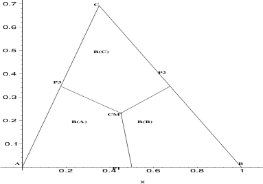
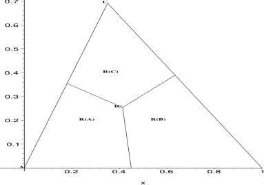
Figure 3: The vertex regions constructed with center of mass $M_{C}$ (left) and incenter $M_{I}$ (right) using the line segments on the line joining $M$ to $\mathcal{Y}_{3}$.

Notice that $r\geq 1$ implies $x\in N_{PE}^{r}(x,M)$ for all $x\in T(\mathcal{Y}_{3})$. Furthermore, $\lim_{r\rightarrow\infty}N_{PE}^{r}(x,M)=T(\mathcal{Y}_{3})$ for all $x\in T(\mathcal{Y}_{3})\setminus\mathcal{Y}_{3}$, so we define $N_{PE}^{\infty}(x,M)=T(\mathcal{Y}_{3})$ for all such $x$. For $x\in\mathcal{Y}_{3}$, we define $N_{PE}^{r}(x,M)=\{x\}$ for all $r\in[1,\infty]$.

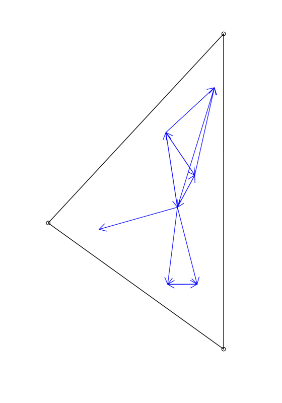
Figure 4: A realization of 7 $\mathcal{X}$ points generated iid $\mathcal{U}(T(\mathcal{Y}_{3}))$ (left) and the corresponding arcs of $r$-factor proportional edge PCD with $r=3/2$ and $M=M_{C}$.

Hence, $r$-factor proportional edge PCD has vertices $\mathcal{X}_{n}$ and arcs $(x_{i},x_{j})$ iff $x_{j}\in N_{PE}^{r}(x_{i},M)$. See Figure 4 for a realization of $\mathcal{X}_{n}$ with $n=7$ and $m=3$. The number of arcs is 12 and $\gamma_{n}(r=2,M_{C})=1$. By construction, note that as $x$ gets closer to $M$ (or equivalently further away from the vertices in vertex regions), $N_{PE}^{r}(x,M)$ increases in area, hence it is more likely for the outdegree of $x$ to increase. So if more $\mathcal{X}$ points are around the center $M$, then it is more likely for $\gamma_{n}$ to decrease, on the other hand, if more $\mathcal{X}$ points are around the vertices $\mathcal{Y}_{3}$, then the regions get smaller, hence it is more likely for the outdegree for such points to be smaller, thereby implying $\gamma_{n}$ to increase. This probabilistic behaviour is utilized in Ceyhan and Priebe, (2005) for testing spatial patterns.

Note also that, $N_{PE}^{r}(x,M)$ is a homothetic transformation (enlargement) with $r\geq 1$ applied on the region $N_{PE}^{r=1}(x,M)$. Furthermore, this transformation is also an affine similarity transformation.

3.2 Some Basic Properties and Auxiliary Concepts

First, notice that $X_{i}\stackrel{{\scriptstyle iid}}{{\sim}}F$, with the additional assumption that the non-degenerate two-dimensional probability density function $f$ exists with support $\mathcal{S}(F)\subseteq T(\mathcal{Y}_{3})$, imply that the special case in the construction of $N_{PE}^{r}$ — $X$ falls on the boundary of two vertex regions — occurs with probability zero. Note that for such an $F$, $N_{PE}^{r}(X)$ is a triangle a.s.

The similarity ratio of $N_{PE}^{r}(x,M)$ to $T(\mathcal{Y}_{3})$ is given by $\frac{\min\Bigl{(}d\bigl{(}v(x),\,e(x)\bigr{)},r\,d\bigl{(}v(x),\,\ell(v(x),x)\bigr{)}\Bigr{)}}{d(v(x),\,e(x))},$ that is, $N_{PE}^{r}(x,M)$ is similar to $T(\mathcal{Y}_{3})$ with the above ratio. Property (1) holds depending on the pair $M$ and $r$. That is, there exists an $r_{0}$ and a corresponding point $M(r_{0})\in T(\mathcal{Y}_{3})^{o}$ so that $N_{PE}^{r_{0}}(x,M)$ satisfies Property (1) for all $r\leq r_{0}$, but fails to satisfy it otherwise. Property (1) fails for all $M$ when $r=\infty$. With $CM$-vertex regions, for all $r\in[1,\infty]$, the area $A\left(N_{PE}^{r}(x,M_{C})\right)$ is a continuous function of $d(\ell_{r}(v(x),x),v(x))$ which is a continuous function of $d(\ell(v(x),x),v(x))$ which is a continuous function of $x$.

Note that if $x$ is close enough to $M$, we might have $N_{PE}^{r}(x,M)=T(\mathcal{Y}_{3})$ for $r=\sqrt{2}$ also.

In $T(\mathcal{Y}_{3})$, drawing the lines $q_{j}(r,x)$ such that $d(\mathsf{y}_{j},e_{j})=r\,d(\mathsf{y}_{j},q_{j}(r,x))$ for $j\in\{1,2,3\}$ yields a triangle, denoted $\mathscr{T}_{r}$, for $r<3/2$ . See Figure 5 for $\mathscr{T}_{r}$ with $r=\sqrt{2}$.

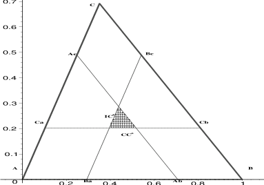
Figure 5: The triangle $\mathscr{T}_{r}$ with $r=\sqrt{2}$ (the hatched region).

The functional form of $\mathscr{T}_{r}$ in the basic triangle $T_{b}$ is given by

$$\mathscr{T}_{r}=T(t_{1}(r),t_{2}(r),t_{3}(r))=\left\{(x,y)\in T_{b}:y\geq\frac{c_{2}\,(r-1)}{r};\;y\leq\frac{c_{2}\,(1-r\,x)}{r\,(1-c_{1})};\;y\leq\frac{c_{2}\,(r\,(x-1)+1)}{r\,c_{1}}\right\}$$ (2)

$$=T\Biggl{(}\left(\frac{(r-1)\,(1+c_{1})}{r},\frac{c_{2}\,(r-1)}{r}\right),\left(\frac{2-r+c_{1}\,(r-1)}{r},\frac{c_{2}\,(r-1)}{r}\right),\left(\frac{c_{1}\,(2-r)+r-1}{r},\frac{c_{2}\,(r-2)}{r}\right)\Biggr{)}.$$

There is a crucial difference between the triangles $\mathscr{T}_{r}$ and $T(M_{1},M_{2},M_{3})$. More specifically $T(M_{1},M_{2},M_{3})\subseteq\mathscr{R}_{S}(r,M)$ for all $M$ and $r\geq 2$, but $(\mathscr{T}_{r})^{o}$ and $\mathscr{R}_{S}(r,M)$ are disjoint for all $M$ and $r$. So if $M\in(\mathscr{T}_{r})^{o}$, then $\mathscr{R}_{S}(r,M)=\emptyset$; if $M\in\partial(\mathscr{T}_{r})$, then $\mathscr{R}_{S}(r,M)=\{M\}$; and if $M\not\in\mathscr{T}_{r}$, then $\mathscr{R}_{S}(r,M)$ has positive area. Thus $N_{PE}^{r}(\cdot,M)$ fails to satisfy Property (1) if $M\not\in\mathscr{T}_{r}$. See Figure 6 for two examples of superset regions with $M$ that corresponds to circumcenter $M_{CC}$ in this triangle and the vertex regions are constructed using orthogonal projections. For $r=2$, note that $\mathscr{T}_{r}=\emptyset$ and the superset region is $T(M_{1},M_{2},M_{3})$ (see Figure 6 (left)), while for $r=\sqrt{2}$, $\mathscr{T}_{r}^{o}$ and $\mathscr{R}_{S}(r=\sqrt{2},M)^{o}$ are disjoint (see Figure 6 (right))

The triangle $\mathscr{T}_{r}$ given in Equation (2) and the superset region $\mathscr{R}_{S}(r,M)$ play a crucial role in computing the distribution of the domination number of the $r$-factor PCD.

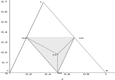
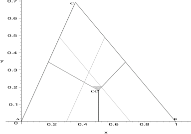
Figure 6: The superset regions (the shaded regions) constructed with circumcenter $M_{CC}$ with $r=\sqrt{2}$ (left) and $r=2$ (right) with vertex regions constructed with orthogonal projections to the edges.

3.3 Main Result

Next, we present the main result of this article. Let $\gamma_{n}(r,M):=\gamma\left(\mathcal{X}_{n},N_{PE}^{r},M\right)$ be the domination number of the PCD based on $N_{PE}^{r}$ with $\mathcal{X}_{n}$, a set of iid random variables from $\mathcal{U}(T(\mathcal{Y}_{3}))$, with $M$-vertex regions.

The domination number $\gamma_{n}(r,M)$ of the PCD has the following asymptotic distribution. As $n\rightarrow\infty$,

$$\gamma_{n}(r,M)\sim\left\{\begin{array}[]{ll}2+\operatorname{BER}(1-p_{r}),&\text{for $r\in[1,3/2]$ and $M\in\{t_{1}(r),t_{2}(r),t_{3}(r)\}$,}\\ 1,&\text{for $r>3/2$,}\\ 3,&\text{for $r\in[1,3/2)$ and $M\in\mathscr{T}_{r}\setminus\{t_{1}(r),t_{2}(r),t_{3}(r)\}$,}\\ \end{array}\right.$$ (3)

where $\operatorname{BER}(p)$ stands for Bernoulli distribution with probability of success $p$, $\mathscr{T}_{r}$ and $t_{j}(r)$ are defined in Equation (2), and for $r\in[1,3/2)$ and $M\in\{t_{1}(r),t_{2}(r),t_{3}(r)\}$,

$$p_{r}=\int_{0}^{\infty}\int_{0}^{\infty}\frac{64\,r^{2}}{9\,(r-1)^{2}}\,w_{1}\,w_{3}\,\exp\left(\frac{4\,r}{3\,(r-1)}\,(w_{1}^{2}+w_{3}^{2}+2\,r\,(r-1)\,w_{1}\,w_{3})\right)\,dw_{3}w_{1};$$ (4)

for example for $r=3/2$ and $M=M_{C}$, $p_{r}\approx.7413$.

In Equation (3), the first line is referred as the non-degenerate case, the second and third lines are referred as degenerate cases with a.s. limits 1 and 3, respectively.

Figure 7: Plotted is the probability $p_{r}=\lim_{n\rightarrow\infty}P\left(\gamma_{n}(r,M)=2\right)$ given in Equation (4) as a function of $r$ for $r\in[1,3/2)$ and $M\in\{t_{1}(r),t_{2}(r),t_{3}(r)\}$.

In the following sections, we define a region associated with $\gamma=1$ case in general. Then we give finite sample and asymptotic upper bounds for $\gamma_{n}(r,M)$. Then we derive the asymptotic distribution of $\gamma_{n}(r,M)$.

4 The $\Gamma_{1}$-Regions for $N_{PE}^{r}$

First, we define $\Gamma_{1}$-regions in general, and describe the construction of $\Gamma_{1}$-region of $N_{PE}^{r}$ for one point and multiple point data sets, and provide some results concerning $\Gamma_{1}$-regions.

4.1 Definition of $\Gamma_{1}$-Regions

Let $(\Omega,\mathcal{M})$ be a measurable space and consider the proximity map $N:\Omega\rightarrow 2^{\Omega}$. For any set $B\subseteq\Omega$, the $\Gamma_{1}$-region of $B$ associated with $N(\cdot)$, is defined to be the region $\Gamma^{N}_{1}(B):=\{z\in\Omega:B\subseteq N(z)\}$. For $x\in\Omega$, we denote $\Gamma^{N}_{1}\bigl{(}\{x\}\bigr{)}$ as $\Gamma^{N}_{1}(x)$.

If $\mathcal{X}_{n}=\bigl{\{}X_{1},X_{2},\cdots,X_{n}\bigr{\}}$ is a set of $\Omega$-valued random variables, then $\Gamma^{N}_{1}(X_{i})$, $i=1,\cdots,n$, and $\Gamma^{N}_{1}(\mathcal{X}_{n})$ are random sets. If the $X_{i}$ are iid, then so are the random sets $\Gamma^{N}_{1}(X_{i})$.

Note that $\gamma(\mathcal{X}_{n},N)=1$ iff $\mathcal{X}_{n}\cap\Gamma^{N}_{1}(\mathcal{X}_{n})\not=\emptyset$. Hence the name $\Gamma_{1}$-region.

It is trivial to see the following.

Proposition 4.1.

For any proximity map $N$ and set $B\subseteq\Omega$, $\mathscr{R}_{S}(N)\subseteq\Gamma^{N}_{1}(B)$.

Lemma 4.2.

For any proximity map $N$ and $B\subseteq\Omega$, $\Gamma^{N}_{1}(B)=\cap_{x\in B}\Gamma^{N}_{1}(x)$.

Proof: Given a particular type of proximity map $N$ and subset $B\subseteq\Omega$, $y\in\Gamma^{N}_{1}(B)$ iff $B\subseteq N(y)$ iff $x\in N(y)$ for all $x\in B$ iff $y\in\Gamma^{N}_{1}(x)$ for all $x\in B$ iff $y\in\cap_{x\in B}\Gamma^{N}_{1}(x)$. Hence the result follows. $\blacksquare$

A problem of interest is finding, if possible, a (proper) subset of $B$, say $G\subsetneq B$, such that $\Gamma^{N}_{1}(B)=\cap_{x\in G}\Gamma^{N}_{1}(x)$. This implies that only the points in $G$ will be active in determining $\Gamma^{N}_{1}(B)$.

For example, in $\mathbb{R}$ with $\mathcal{Y}_{2}=\{0,1\}$, and $\mathcal{X}_{n}$ a set of iid random variables of size $n>1$ from $F$ in $(0,1)$, $\Gamma^{N_{S}}_{1}(\mathcal{X}_{n})=\Bigl{(}X_{n:n}/2,(1+X_{1:n})/2\Bigr{)}$. So the extrema (minimum and maximum) of the set $\mathcal{X}_{n}$ are sufficient to determine the $\Gamma_{1}$-region; i.e., $G=\{X_{1:n},X_{n:n}\}$ for $\mathcal{X}_{n}$ a set of iid random variables from a continuous distribution on $(0,1)$. Unfortunately, in the multi-dimensional case, there is no natural ordering that yields natural extrema such as minimum or maximum.

4.2 Construction of $\Gamma_{1}$-Region of a Point for $N_{PE}^{r}$

For $N_{PE}^{r}(\cdot,M)$, the $\Gamma_{1}$-region, denoted as $\Gamma^{r}_{1}(\cdot,M):=\Gamma^{N_{PE}^{r}}_{1}(\cdot,M)$, is constructed as follows; see also Figure 8. Let $\xi_{j}(r,x)$ be the line parallel to $e_{j}$ such that $\xi_{j}(r,x)\cap T(\mathcal{Y}_{3})\not=\emptyset$ and $r\,d(\mathsf{y}_{j},\xi_{j}(r,x))=d(\mathsf{y}_{j},\ell(\mathsf{y}_{j},x))$ for $j\in\{1,2,3\}$. Then

$$\Gamma^{r}_{1}(x,M)=\cup_{j=1}^{3}\bigl{[}\Gamma^{r}_{1}(x,M)\cap R_{M}(\mathsf{y}_{j})\bigr{]}$$

where $\Gamma^{r}_{1}(x,M)\cap R_{M}(\mathsf{y}_{j})=\{z\in R_{M}(\mathsf{y}_{j}):d(\mathsf{y}_{j},\ell(\mathsf{y}_{j},z))\geq d(\mathsf{y}_{j},\xi_{j}(r,x)\}\text{ for }j\in\{1,2,3\}.$

Notice that $r\geq 1$ implies that $x\in\Gamma^{r}_{1}(x,M)$. Furthermore, $\lim_{r\rightarrow\infty}\Gamma^{r}_{1}(x,M)=T(\mathcal{Y}_{3})$ for all $x\in T(\mathcal{Y}_{3})\setminus\mathcal{Y}_{3}$ and so we define $\Gamma^{r=\infty}_{1}(x,M)=T(\mathcal{Y}_{3})$ for all such $x$. For $x\in\mathcal{Y}_{3}$, $\Gamma^{r}_{1}(x,M)=\{x\}$ for all $r\in[1,\infty]$.

Figure 8: Construction of the $\Gamma_{1}$-region, $\Gamma^{r=2}_{1}(x,M_{C})$ (shaded region).

Notice that $\Gamma^{r}_{1}(x,M_{C})$ is a convex hexagon for all $r\geq 2$ and $x\in T(\mathcal{Y}_{3})\setminus\mathcal{Y}_{3}$, (since for such an $x$, $\Gamma^{r}_{1}(x,M_{C})$ is bounded by $\xi_{j}(r,x)$ and $e_{j}$ for all $j\in\{1,2,3\}$, see also Figure 8,) else it is either a convex hexagon or a non-convex but star-shaped polygon depending on the location of $x$ and the value of $r$.

4.3 The $\Gamma_{1}$-Region of a Multiple Point Data Set for $N_{PE}^{r}$

So far, we have described the $\Gamma_{1}$-region for a point in $x\in T(\mathcal{Y}_{3})$. For a set $\mathcal{X}_{n}$ of size $n$ in $T(\mathcal{Y}_{3})$, the region $\Gamma^{r}_{1}(\mathcal{X}_{n},M)$ can be specified by the edge extrema only. The (closest) edge extrema of a set $B$ in $T(\mathcal{Y}_{3})$ are the points closest to the edges of $T(\mathcal{Y}_{3})$, denoted $x_{e_{j}}$ for $j\in\{1,2,3\}$; that is, $x_{e_{j}}\in\operatorname{arginf}_{x\in B}d(x,e_{j})$. Note that if $B=\mathcal{X}_{n}$ is a set of iid random variables of size $n$ from $F$ then the edge extrema, denoted $X_{e_{j}}(n)$, are random variables. Below, we show that the edge extrema are the active points in defining $\Gamma^{r}_{1}(\mathcal{X}_{n},M)$.

Proposition 4.3.

Let $B$ be any set of $n$ distinct points in $T(\mathcal{Y}_{3})$. For $r$-factor proportional-edge proximity maps with $M$-vertex regions, $\Gamma^{r}_{1}\left(B,M\right)=\cap_{k=1}^{3}\,\Gamma^{r}_{1}\left(x_{e_{k}},M\right)$.

Proof: Given $B=\{x_{1},\ldots,x_{n}\}$ in $T(\mathcal{Y}_{3})$. Note that

$$\Gamma^{r}_{1}(B,M)\cap R_{M}(\mathsf{y}_{j})=\bigl{[}\cap_{i=1}^{n}\,\Gamma^{r}_{1}(x_{i},M)\bigr{]}\cap R_{M}(\mathsf{y}_{j}),$$

but by definition $x_{e_{j}}\in\operatorname{argmax}_{x\in B}d(\mathsf{y}_{j},\xi_{j}(r,x))$, so

$$\Gamma^{r}_{1}(B,M)\cap R_{M}(\mathsf{y}_{j})=\Gamma^{r}_{1}(x_{e_{j}},M)\cap R_{M}(\mathsf{y}_{j})\text{ for }j\in\{1,2,3\}.$$ (5)

Furthermore, $\Gamma^{r}_{1}(B,M)=\cup_{j=1}^{3}\bigl{[}\Gamma^{r}_{1}(x_{e_{j}},M)\cap R_{M}(\mathsf{y}_{j})\bigr{]}$, and

$$\Gamma^{r}_{1}(x_{e_{j}},M)\cap R_{M}(\mathsf{y}_{j})=\cap_{k=1}^{3}\bigl{[}\Gamma^{r}_{1}(x_{e_{k}},M)\cap R_{M}(\mathsf{y}_{j})\bigr{]}\text{ for }j\in\{1,2,3\}.$$ (6)

Combining these two results in Equations (5) and (6), we obtain $\Gamma^{r}_{1}(B,M)=\cap_{k=1}^{3}\,\Gamma^{r}_{1}(x_{e_{k}},M)$. $\blacksquare$

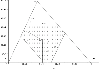
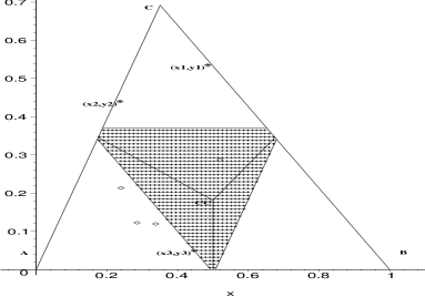
Figure 9: The $\Gamma_{1}$-regions (the hatched regions) for $r=2$ with seven $\mathcal{X}$ points iid $\mathcal{U}(T(\mathcal{Y}_{3}))$ where vertex regions constructed with incenter $M_{I}$ (left) and circumcenter $M_{CC}$ (right) with orthogonal projection.

From the above proposition, we see that the $\Gamma_{1}$-region for $B$ as in proposition can also be written as the union of three regions of the form

$$\Gamma^{r}_{1}(B,M)\cap R_{M}(\mathsf{y}_{j})=\{z\in R_{M}(\mathsf{y}_{j}):\;d(\mathsf{y}_{j},\ell(\mathsf{y}_{j},z))\geq d(\mathsf{y}_{j},\xi_{j}(r,x_{e_{j}}))\}\text{ for }j\in\{1,2,3\}.$$

See Figure 9 for $\Gamma_{1}$-region for $r=2$ with seven $\mathcal{X}$ points iid $\mathcal{U}(T(\mathcal{Y}_{3}))$. In the left figure, vertex regions are based on incenter, while in the right figure, on circumcenter with orthogonal projections to the edges. In either case $\mathcal{X}_{n}\cap\Gamma^{r=2}_{1}(\mathcal{X}_{n},M)$ is nonempty, hence $\gamma_{n}(2,M)=1$.

Below, we demonstrate that edge extrema are distinct with probability 1 as $n\rightarrow\infty$. Hence in the limit three distinct points suffice to determine the $\Gamma_{1}$-region.

Theorem 4.4.

Let $\mathcal{X}_{n}$ be a set of iid random variables from $\mathcal{U}(T(\mathcal{Y}_{3}))$ and let $E_{c,3}(n)$ be the event that (closest) edge extrema are distinct. Then $P(E_{c,3}(n))\rightarrow 1$ as $n\rightarrow\infty$.

We can also define the regions associated with $\gamma(\mathcal{X}_{n},N)=k$ for $k\leq n$ called $\Gamma_{k}$-region for proximity map $N_{\mathcal{Y}_{3}}(\cdot)$ and set $B\subseteq\Omega$ for $k=1,\ldots,n$ (see Ceyhan, (2004)).

5 The Asymptotic Distribution of $\gamma_{n}(r,M)$

In this section, we first present a finite sample upper bound for $\gamma_{n}(r,M)$, then present the degenerate cases, and the nondegenerate case of the asymptotic distribution of $\gamma_{n}(r,M)$ given in Equation (3).

5.1 An Upper Bound for $\gamma_{n}(r,M)$

Recall that by definition, $\gamma(\mathcal{X}_{n},N)\leq n$. We will seek an a.s. least upper bound for $\gamma(\mathcal{X}_{n},N)$. Let $\mathcal{X}_{n}$ be a set of iid random variables from $F$ on $T(\mathcal{Y}_{3})$ and let $\gamma(\mathcal{X}_{n},N)$ be the domination number for the PCD based on a proximity map $N$. Denote the general a.s. least upper bound for $\gamma(\mathcal{X}_{n},N)$ that works for all $n\geq 1$ and is independent of $n$ (which is called $\kappa$-value in Ceyhan, (2004)) as $\kappa(N):=\min\{k:\gamma(\mathcal{X}_{n},N)\leq k\text{ a.s. for all }n\geq 1\}$.

In $\mathbb{R}$ with $\mathcal{Y}_{2}=\{0,1\}$, for $\mathcal{X}_{n}$ a set of iid random variables from $\mathcal{U}(0,1)$, $\gamma(\mathcal{X}_{n},N_{S})\leq 2$ with equality holding with positive probability. Hence $\kappa(N_{S})=2$.

Theorem 5.1.

Let $\mathcal{X}_{n}$ be a set of iid random variables from $\mathcal{U}(T(\mathcal{Y}_{3}))$ and $M\in\mathbb{R}^{2}\setminus\mathcal{Y}_{3}$. Then $\kappa\left(N_{PE}^{r}\right)=3$ for $N_{PE}^{r}(\cdot,M)$.

Proof: For $N_{PE}^{r}(\cdot,M)$, pick the point closest to edge $e_{j}$ in vertex region $R_{M}(\mathsf{y}_{j})$; that is, pick $U_{j}\in\operatorname{argmin}_{X\in\mathcal{X}_{n}\cap R_{M}(\mathsf{y}_{j})}d(X,e_{j})=\operatorname{argmax}_{X\in\mathcal{X}_{n}\cap R_{M}(\mathsf{y}_{j})}d(\ell(\mathsf{y},X),\mathsf{y}_{j})$ in the vertex region for which $X_{n}\cap R_{M}(\mathsf{y}_{j})\not=\emptyset$ for $j\in\{1,2,3\}$ (note that as $n\rightarrow\infty$, $U_{j}$ is unique a.s. for each $j$, since $X$ is from $\mathcal{U}(T(\mathcal{Y}_{3}))$). Then $\mathcal{X}_{n}\cap R_{M}(\mathsf{y}_{j})\subset N_{PE}^{r}(U_{j},M)$. Hence $\mathcal{X}_{n}\subset\cup_{j=1}^{3}N_{PE}^{r}(U_{j},M)$. So $\gamma_{n}(r,M_{C})\leq 3$ with equality holding with positive probability. Thus $\kappa\left(N_{PE}^{r}\right)=3$. $\blacksquare$

Below is a general result for the limiting distribution of $\gamma(\mathcal{X}_{n},N)$ for $\mathcal{X}_{n}$ from a very broad family of distributions and for general $N(\cdot)$.

Lemma 5.2.

Let $\mathscr{R}_{S}(N)$ be the superset region for the proximity map $N(\cdot)$ and $\mathcal{X}_{n}$ be a set of iid random variables from $F$ with $P_{F}(X\in\mathscr{R}_{S}(N))>0$. Then $\lim_{n\rightarrow\infty}P_{F}(\gamma(\mathcal{X}_{n},N)=1)=1$.

Proof: Suppose $P_{F}(X\in\mathscr{R}_{S}(N))>0$. Recall that for any $x\in\mathscr{R}_{S}(N)$, we have $N(x)=\Omega$, so $\mathcal{X}_{n}\subseteq N(x)$, hence if $\mathcal{X}_{n}\cap\mathscr{R}_{S}(N)\not=\emptyset$ then $\gamma(\mathcal{X}_{n},N)=1$. Then $P(\mathcal{X}_{n}\cap\mathscr{R}_{S}(N)\not=\emptyset)\leq P(\gamma(\mathcal{X}_{n},N)=1)$. But $P\bigl{(}\mathcal{X}_{n}\cap\mathscr{R}_{S}(N)\not=\emptyset\bigr{)}=1-P\bigl{(}\mathcal{X}_{n}\cap\mathscr{R}_{S}(N)=\emptyset\bigr{)}=1-\bigl{[}1-P_{F}\bigl{(}X\in\mathscr{R}_{S}(N)\bigr{)}\bigr{]}^{n}\rightarrow 1\text{ as }n\rightarrow\infty,$ since $P_{F}\bigl{(}X\in\mathscr{R}_{S}(N)\bigr{)}>0$. Hence $\lim_{n\rightarrow\infty}P(\gamma(\mathcal{X}_{n},N)=1)=1$. $\blacksquare$

Remark 5.3.

In particular, for $F=\mathcal{U}(T(\mathcal{Y}_{3}))$, the inequality $P_{F}(X\in\mathscr{R}_{S}(N))>0$ holds iff $A(\mathscr{R}_{S}(N))>0$, then $P(\mathcal{X}_{n}\cap\mathscr{R}_{S}(N)\not=\emptyset)\rightarrow 1$. $\square$

For $\mathcal{Y}_{2}=\{0,1\}\subset\mathbb{R}$, $\mathscr{R}_{S}(N_{S})=\{1/2\}$, so Lemma 5.2 does not apply to $N_{S}$ in $\mathbb{R}$.

Recall that $\kappa\left(N_{PE}^{r}\right)=3$, then

$$1\leq\mathbf{E}\,\left[\gamma_{n}(r,M)\right]\leq 3\text{ and }0\leq\mathbf{Var}\,\left[\gamma_{n}(r,M)\right]\leq 9/4.$$

Furthermore, there is a stochastic ordering for $\gamma_{n}(r,M)$.

Theorem 5.4.

Suppose $\mathcal{X}_{n}$ is a set of iid random variables from a continuous distribution $F$ on $T(\mathcal{Y}_{3})$. Then for $r_{1}<r_{2}$, we have $\gamma_{n}(r_{2},M)\leq^{ST}\gamma\left(\mathcal{X}_{n},N_{PE}^{r_{1}},M\right)$.

Proof: Suppose $r_{1}<r_{2}$. Then $P\left(\gamma_{n}(r_{2},M)\leq 1\right)>P\left(\gamma_{n}(r_{1},M)\leq 1\right)$ since $\Gamma^{r_{1}}_{1}(\mathcal{X}_{n},M)\subsetneq\Gamma^{r_{2}}_{1}(\mathcal{X}_{n},M)$ for any realization of $\mathcal{X}_{n}$ and by a similar argument $P\bigl{(}\gamma_{n}(r_{2},M)\leq 2\bigr{)}>P\left(\gamma_{n}(r_{1},M)\leq 2\right)$ so $P\left(\gamma_{n}(r_{2},M)\leq 3\right)=P\left(\gamma_{n}(r_{1},M)\leq 3\right).$ Hence the desired result follows. $\blacksquare$

5.2 Geometry Invariance

We present a “geometry invariance” result for $N_{PE}^{r}(\cdot,M)$ where $M$-vertex regions are constructed using the lines joining $\mathcal{Y}_{3}$ to $M$, rather than the orthogonal projections from $M$ to the edges. This invariance property will simplify the notation in our subsequent analysis by allowing us to consider the special case of the equilateral triangle.

Theorem 5.5.

(Geometry Invariance Property) Suppose $\mathcal{X}_{n}$ is a set of iid random variables from $\mathcal{U}(T(\mathcal{Y}_{3}))$. Then for any $r\in[1,\infty]$ the distribution of $\gamma_{n}(r,M)$ is independent of $\mathcal{Y}_{3}$ and hence the geometry of $T(\mathcal{Y}_{3})$.

Proof: Suppose $X\sim\mathcal{U}(T(\mathcal{Y}))$. A composition of translation, rotation, reflections, and scaling will take any given triangle $T(\mathcal{Y})=T(\mathsf{y}_{1},\mathsf{y}_{2},\mathsf{y}_{3})$ to the basic triangle $T_{b}=T((0,0),(1,0),(c_{1},c_{2}))$ with $0<c_{1}\leq 1/2$, $c_{2}>0$, and $(1-c_{1})^{2}+c_{2}^{2}\leq 1$. Furthermore, when $X$ is also transformed in the same manner, say to $X^{\prime}$, then $X^{\prime}$ is uniform on $T_{b}$, i.e., $X^{\prime}\sim\mathcal{U}(T_{b})$. The transformation $\phi_{e}:\mathbb{R}^{2}\rightarrow\mathbb{R}^{2}$ given by $\phi_{e}(u,v)=\left(u+\frac{1-2\,c_{1}}{\sqrt{3}}\,v,\frac{\sqrt{3}}{2\,c_{2}}\,v\right)$ takes $T_{b}$ to the equilateral triangle $T_{e}=\bigl{(}(0,0),(1,0),(1/2,\sqrt{3}/2)\bigr{)}$. Investigation of the Jacobian shows that $\phi_{e}$ also preserves uniformity. That is, $\phi_{e}(X^{\prime})\sim\mathcal{U}(T_{e})$. Furthermore, the composition of $\phi_{e}$, with the scaling and rigid body transformations, maps the boundary of the original triangle, $T_{o}$, to the boundary of the equilateral triangle, $T_{e}$, the lines joining $M$ to $\mathsf{y}_{j}$ in $T_{b}$ to the lines joining $\phi_{e}(M)$ to $\phi_{e}(\mathsf{y}_{j})$ in $T_{e}$, and lines parallel to the edges of $T_{o}$ to lines parallel to the edges of $T_{e}$. Since the distribution of $\gamma_{n}(r,M)$ involves only probability content of unions and intersections of regions bounded by precisely such lines and the probability content of such regions is preserved since uniformity is preserved; the desired result follows. $\blacksquare$

Note that geometry invariance of $\gamma\left(\mathcal{X}_{n},N_{PE}^{r=\infty},M\right)$ also follows trivially, since for $r=\infty$, we have $\gamma_{n}(r=\infty,M)=1$ a.s. for all $\mathcal{X}_{n}$ from any $F$ with support in $T(\mathcal{Y}_{3})\setminus\mathcal{Y}_{3}$.

Based on Theorem 5.5 we may assume that $T(\mathcal{Y}_{3})$ is a standard equilateral triangle with
$\mathcal{Y}_{3}=\left\{(0,0),(1,0),\left(1/2,\sqrt{3}/2\right)\right\}$ for $N_{PE}^{r}(\cdot,M)$ with $M$-vertex regions.

Notice that, we proved the geometry invariance property for $N_{PE}^{r}$ where $M$-vertex regions are defined with the lines joining $\mathcal{Y}_{3}$ to $M$. On the other hand, if we use the orthogonal projections from $M$ to the edges, the vertex regions, hence $N_{PE}^{r}$ will depend on the geometry of the triangle. That is, the orthogonal projections from $M$ to the edges will not be mapped to the orthogonal projections in the standard equilateral triangle. Hence with the choice of the former type of $M$-vertex regions, it suffices to work on the standard equilateral triangle. On the other hand, with the orthogonal projections, the exact and asymptotic distribution of $\gamma_{n}$ will depend on $c_{1},c_{2}$, so one needs to do the calculations for each possible combination of $c_{1},c_{2}$.

5.3 The Degenerate Case with $\gamma_{n}(r,M)\stackrel{{\scriptstyle p}}{{\rightarrow}}1$

Below, we prove that $\gamma_{n}(r,M)$ is degenerate in the limit for $r>3/2$.

Theorem 5.6.

Suppose $\mathcal{X}_{n}$ is a set of iid random variables from a continuous distribution $F$ on $T(\mathcal{Y}_{3})$. If $M\not\in\mathscr{T}_{r}$ (see Figure 5 and Equation (2) for $\mathscr{T}_{r}$), then $\lim_{n\rightarrow\infty}P\left(\gamma_{n}(r,M)=1\right)=1$ for all $M\in\mathbb{R}^{2}\setminus\mathcal{Y}_{3}$.

Proof: Suppose $M\notin\mathscr{T}_{r}$. Then $\mathscr{R}_{S}\left(N_{PE}^{r},M\right)$ is nonempty with positive area. Hence the result follows by Lemma 5.2. $\blacksquare$

Corollary 5.7.

Suppose $\mathcal{X}_{n}$ is a set of iid random variables from a continuous distribution $F$ on $T(\mathcal{Y}_{3})$. Then for $r>3/2$, $\lim_{n\rightarrow\infty}P\left(\gamma_{n}(r,M)=1\right)=1$ for all $M\in R^{2}\setminus\mathcal{Y}_{3}$.

Proof: For $r>3/2$, $\mathscr{T}_{r}=\emptyset$, so $M\not\in\mathscr{T}_{r}$. Hence the result follows by Theorem 5.6. $\blacksquare$

We estimate the distribution of $\gamma_{n}(r,M)$ with $r=2$ and $M=M_{C}$ for various $n$ empirically. In Table 1 (left), we present the empirical estimates of $\gamma_{n}(r,M)$ with $n=10,\,20,\,30,\,50,\,100$ based on $1000$ Monte Carlo replicates in $T_{e}$. Observe that the empirical estimates are in agreement with the asymptotic distribution given in Corollary 5.7.

$k\diagdown n$ 10 20 30 50 100 1 961 1000 1000 1000 1000 2 34 0 0 0 0 3 5 0 0 0 0

$k\diagdown n$ 10 20 30 50 100 1 9 0 0 0 0 2 293 110 30 8 0 3 698 890 970 992 1000

Table 1: The number of $\gamma_{n}(r,M)=k$ out of $N=1000$ Monte Carlo replicates with $M=M_{C}$ and $r=2$ (left) and $r=5/4$ (right).

The asymptotic distribution of $\gamma_{n}(r,M)$ for $r<3/2$ depends on the relative position of $M$ with respect to the triangle $\mathscr{T}_{r}$.

5.4 The Degenerate Case with $\gamma_{n}(r,M)\stackrel{{\scriptstyle p}}{{\rightarrow}}3$

Theorem 5.8.

Suppose $\mathcal{X}_{n}$ is a set of iid random variables from a continuous distribution $F$ on $T(\mathcal{Y}_{3})$. If $M\in(\mathscr{T}_{r})^{o}$, then $P\left(\gamma_{n}(r,M)=3\right)\rightarrow 1$ as $n\rightarrow\infty$.

We estimate the distribution of $\gamma_{n}(r,M)$ with $r=5/4$ and $M=M_{C}$ for various $n$ values empirically. In Table 1 (right), we present the empirical estimates of $\gamma_{n}(r,M)$ with $n=10,\,20,\,30,\,50,\,100$ based on $1000$ Monte Carlo replicates in $T_{e}$. Observe that the empirical estimates are in agreement with our result in Theorem 5.8.

Theorem 5.9.

Suppose $\mathcal{X}_{n}$ is a set of iid random variables from $\mathcal{U}(T(\mathcal{Y}_{3}))$. If $M\in\partial(\mathscr{T}_{r})$, then $P\left(\gamma_{n}(r,M)>1\right)\rightarrow 1$ as $n\rightarrow\infty$.

For $M\in\partial(\mathscr{T}_{r})$, there are two separate cases:

• $M\in\partial(\mathscr{T}_{r})\setminus\{t_{1}(r),\,t_{2}(r),\,t_{3}(r)\}$ where $t_{j}(r)$ with $j\in\{1,2,3\}$ are the vertices of $\mathscr{T}_{r}$ whose explicit forms are given in Equation (2).

• $M\in\{t_{1}(r),\,t_{2}(r),\,t_{3}(r)\}$.

Theorem 5.10.

Suppose $\mathcal{X}_{n}$ is a set of iid random variables from $\mathcal{U}(T(\mathcal{Y}_{3}))$. If $M\in\partial(\mathscr{T}_{r})\setminus\{t_{1}(r),\,t_{2}(r),\,t_{3}(r)\}$, then $P\left(\gamma_{n}(r,M)=3\right)\rightarrow 1$ as $n\rightarrow\infty$.

We estimate the distribution of $\gamma_{n}(r,M)$ with $r=5/4$ and $M=\left(3/5,\sqrt{3}/10\right)\in\partial(\mathscr{T}_{r})\setminus\{t_{1}(r),\,t_{2}(r),\,t_{3}(r)\}$ for various $n$ empirically. In Table 2 we present empirical estimates of $\gamma_{n}(r,M)$ with $n=10,\,20,\,30,\,50,\,100,\,500,\\ \,1000,\,2000$ based on $1000$ Monte Carlo replicates in $T_{e}$. Observe that the empirical estimates are in agreement with our result in Theorem 5.10.

$k\diagdown n$	10	20	30	50	100	500	1000	2000
1	118	60	51	39	15	1	2	1
2	462	409	361	299	258	100	57	29
3	420	531	588	662	727	899	941	970

Table 2: The number of $\gamma_{n}(r,M)=k$ out of $N=1000$ Monte Carlo replicates with $r=5/4$ and $M=\left(3/5,\sqrt{3}/10\right)$.

5.5 The Nondegenerate Case

Theorem 5.11.

Suppose $\mathcal{X}_{n}$ is a set of iid random variables from $\mathcal{U}(T(\mathcal{Y}_{3}))$. If $M\in\{t_{1}(r),\,t_{2}(r),\,t_{3}(r)\}$, then $P\left(\gamma_{n}(r,M)=2\right)\rightarrow p_{r}$ as $n\rightarrow\infty$ where $p_{r}\in(0,1)$ is provided in Equation (4) but only numerically computable.

For example, $p_{r=5/4}\approx.6514$ and $p_{r=\sqrt{2}}\approx.4826$.

So the asymptotic distribution of $\gamma_{n}(r,M)$ with $r\in[1,3/2)$ and $M\in\{t_{1}(r),t_{2}(r),t_{3}(r)\}$ is given by

$$\gamma_{n}(r,M)\sim 2+\operatorname{BER}(1-p_{r}).$$ (7)

We estimate the distribution of $\gamma_{n}(r,M)$ with $r=5/4$ and $M=\left(7/10,\sqrt{3}/10\right)$ for various $n$ empirically. In Table 3, we present the empirical estimates of $\gamma_{n}(r,M)$ with $n=10,\,20,\,30,\,50,\,100,\,500,\,1000,\,2000$ based on $1000$ Monte Carlo replicates in $T_{e}$. Observe that the empirical estimates are in agreement with our result $p_{r=5/4}\approx.6514$.

$k\diagdown n$	10	20	30	50	100	500	1000	2000
1	174	118	82	61	22	5	1	1
2	532	526	548	561	611	617	633	649
3	294	356	370	378	367	378	366	350

Table 3: The number of $\gamma_{n}(r,M)=k$ out of $N=1000$ Monte Carlo replicates with $r=5/4$ and $M=\left(7/10,\sqrt{3}/10\right)$.

Remark 5.12.

For $r=3/2$, as $n\rightarrow\infty$, $P\left(\gamma_{n}(r,M_{C})>1\right)\rightarrow 1$ at rate $O\left(n^{-1}\right)$. $\square$

Theorem 5.13.

Suppose $\mathcal{X}_{n}$ is a set of iid random variables from $\mathcal{U}(T(\mathcal{Y}_{3}))$. Then for $r=3/2$, as $n\rightarrow\infty$,

$$\gamma_{n}(3/2,M_{C})\sim 2+\operatorname{BER}(p\approx.2487)$$ (8)

For the proof of Theorem 5.13, see Ceyhan and Priebe, (2004, 2005).

Using Theorem 5.13,

$$\lim_{n\rightarrow\infty}\mathbf{E}\,\left[\gamma_{n}(3/2,M_{C})\right]=3-p_{3/2}\approx 2.2587$$ (9)

and

$$\lim_{n\rightarrow\infty}\mathbf{Var}\,\left[\gamma_{n}(3/2,M_{C})\right]=6+p_{3/2}-p_{3/2}^{2}\approx.1917.$$ (10)

Indeed, the finite sample distribution of $\gamma_{n}(3/2,M_{C})$ hence the finite sample mean and variance can also be obtained by numerical methods.

We also estimate the distribution of $\gamma_{n}(3/2,M_{C})$ for various $n$ values empirically. The empirical estimates for $n=10,\,20,30,\,50,\,100,\,500,\,1000,\,2000$ based on $1000$ Monte Carlo replicates are given in Table 4. estimates are in agreement with our result $p_{r=3/2}\approx.7413$.

$k\diagdown n$	10	20	30	50	100	500	1000	2000
1	151	82	61	50	27	2	3	1
2	602	636	688	693	718	753	729	749
3	247	282	251	257	255	245	268	250

Table 4: The number of $\gamma_{n}(3/2,M_{C})=k$ out of $N=1000$ Monte Carlo replicates.

5.6 Distribution of the $\gamma_{n}(r,M)$ in Multiple Triangles

So far we have worked with data in one Delaunay triangle, i.e., $m=3$ or $J_{3}=1$. In this section, we present the asymptotic distribution of the domination number of $r$-factor PCDs in multiple Delaunay triangles. Suppose $\mathcal{Y}_{m}=\{\mathsf{y}_{1},\mathsf{y}_{2},\ldots,\mathsf{y}_{m}\}\subset\mathbb{R}^{2}$ be a set of $m$ points in general position with $m>3$ and no more than 3 points are cocircular. Then there are $J_{m}>1$ Delaunay triangles each of which is denoted as $\mathcal{T}_{j}$. Let $M^{j}$ be the point in $\mathcal{T}_{j}$ that corresponds to $M$ in $T_{e}$, $\mathscr{T}_{r}^{j}$ be the triangle that corresponds to $\mathscr{T}_{r}$ in $T_{e}$, and $t_{i}^{j}(r)$ be the vertices of $\mathscr{T}_{r}^{j}$ that correspond to $t_{i}(r)$ in $T_{e}$ for $i\in\{1,2,3\}$. Moreover, let $n_{j}:=|\mathcal{X}_{n}\cap\mathcal{T}_{j}|$, the number of $X$ points in Delaunay triangle $\mathcal{T}_{j}$. For $\mathcal{X}_{n}\subset\mathcal{C}_{H}(\mathcal{Y}_{m})$, let $\gamma_{n_{j}}(r,M^{j})$ be the domination number of the digraph induced by vertices of $\mathcal{T}_{j}$ and $\mathcal{X}_{n}\cap\mathcal{T}_{j}$. Then the domination number of the $r$-factor PCD in $J_{m}$ triangles is

$$\gamma_{n}(r,M,J_{m})=\sum_{j=1}^{J_{m}}\gamma_{n_{j}}(r,M^{j}).$$

See Figure 10 (left) for the 77 $\mathcal{X}$ points that are in $\mathcal{C}_{H}(\mathcal{Y}_{m})$ out of the 200 $\mathcal{X}$ points plotted in Figure 1. Observe that 10 $\mathcal{Y}$ points yield $J_{10}=13$ Delaunay triangles. In Figure 10 (right) are the corresponding arcs for $M=M_{C}$ and $r=3/2$. The corresponding $\gamma_{n}=22$. Suppose $\mathcal{X}_{n}$ is a set of iid random variables from $\mathcal{U}(\mathcal{C}_{H}(\mathcal{Y}_{m}))$, the uniform distribution on convex hull of $\mathcal{Y}_{m}$ and we construct the $r$-factor PCDs using the points $M^{j}$ that correspond to $M$ in $T_{e}$. Then for fixed $m$ (or fixed $J_{m}$), as $n\rightarrow\infty$, so does each $n_{j}$. Furthermore, as $n\rightarrow\infty$, each component $\gamma_{n_{j}}(r,M^{j})$ become independent. Therefore using Equation (3), we can obtain the asymptotic distribution of $\gamma_{n}(r,M,J_{m})$. As $n\rightarrow\infty$, for fixed $J_{m}$,

$$\gamma_{n}(r,M,J_{m})\sim\left\{\begin{array}[]{ll}2\,J_{m}+\operatorname{BIN}(J_{m},1-p_{r}),&\text{for $M^{j}\in\{t^{j}_{1}(r),t^{j}_{2}(r),t^{j}_{3}(r)\}$ and $r\in[1,3/2]$,}\\ J_{m},&\text{for $r>3/2$,}\\ 3\,J_{m},&\text{for $M\in\mathscr{T}_{r}^{j}\setminus\{t^{j}_{1}(r),t^{j}_{2}(r),t^{j}_{3}(r)\}$ and $r\in[1,3/2)$,}\\ \end{array}\right.$$ (11)

where $\operatorname{BIN}(n,p)$ stands for binomial distribution with $n$ trials and probability of success $p$, for $r\in[1,3/2)$ and $M\in\{t_{1}(r),t_{2}(r),t_{3}(r)\}$, $p_{r}$ is given in Equation 3 and for $r=3/2$ and $M=M_{C}$, $p_{r}\approx.7413$ (see Equation (8)).

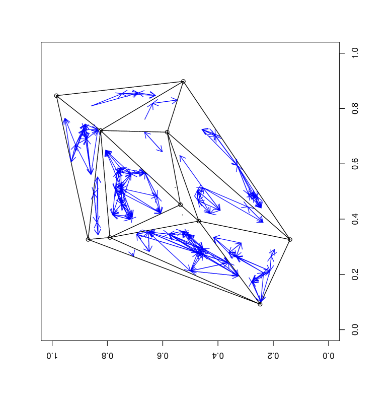
Figure 10: The 77 $\mathcal{X}$ points (crosses) in the convex hull of $\mathcal{Y}$ points (circles) given in Figure 1 (left) and the corresponding arcs (right) of $r$-factor proportional edge PCD with $r=3/2$ and $M=M_{C}$.

5.7 Extension of $N_{PE}^{r}$ to Higher Dimensions

The extension to $\mathbb{R}^{d}$ for $d>2$ with $M=M_{C}$ is provided in Ceyhan and Priebe, (2005), but the extension for general $M$ is similar.

Let $\gamma_{n}(r,M,d):=\gamma(\mathcal{X}_{n},N_{PE}^{r},M,d)$ be the domination number of the PCD based on the extension of $N_{PE}^{r}(\cdot,M)$ to $\mathbb{R}^{d}$. Then it is easy to see that $\gamma_{n}(r,M,3)$ is nondegenerate as $n\rightarrow\infty$ for $r=4/3$. In $\mathbb{R}^{d}$, it can be seen that $\gamma_{n}(r,M,d)$ is nondegenerate in the limit only when $r=(d+1)/d$. Furthermore, for large $d$, asymptotic distribution of $\gamma_{n}(r,M,d)$ is nondegenerate at values of $r$ closer to $1$. Moreover, it can be shown that $\lim_{n\rightarrow\infty}P\bigl{(}2\leq\gamma_{n}(r=(d+1)/d,M,d)\leq d+1\bigr{)}=1$ and we conjecture the following.

Conjecture 5.14.

Suppose $\mathcal{X}_{n}$ is set of iid random variables from the uniform distribution on a simplex in $\mathbb{R}^{d}$. Then the domination number $\gamma_{n}(r,M)$ in the simplex satisfies

$$\lim_{n\rightarrow\infty}P\left(d\leq\gamma_{n}((d+1)/d,M,d)\leq d+1\right)=1.$$

For instance, with $d=3$ we estimate the empirical distribution of $\gamma(\mathcal{X}_{n},4/3)$ for various $n$. The empirical estimates for $n=10,\,20,\,30,\,40,\,50,\,100,\,200,\,500,\,1000,\,2000$ based on $1000$ Monte Carlo replicates for each $n$ are given in Table 5.

$k\diagdown n$	10	20	30	40	50	100	200	500	1000	2000
1	52	18	5	5	4	0	0	0	0	0
2	385	308	263	221	219	155	88	41	31	19
3	348	455	557	609	621	725	773	831	845	862
4	215	219	175	165	156	120	139	128	124	119

Table 5: The number of $\gamma_{n}(4/3,M_{C})=k$ out of $N=1000$ Monte Carlo replicates.

6 Discussion

The $r$-factor proportional-edge proximity catch digraphs (PCDs), when compared to class cover catch digraphs (CCCDs), have some advantages. The asymptotic distribution of the domination number $\gamma_{n}(r,M)$ of the $r$-factor PCDs, unlike that of CCCDs, is mathematically tractable (computable by numerical integration). A minimum dominating set can be found in polynomial time for $r$-factor PCDs in $\mathbb{R}^{d}$ for all $d\geq 1$, but finding a minimum dominating set is an NP-hard problem for CCCDs (except for $\mathbb{R}$). These nice properties of $r$-factor PCDs are due to the geometry invariance of distribution of $\gamma_{n}(r,M)$ for uniform data in triangles.

On the other hand, CCCDs are easily extendable to higher dimensions and are defined for all $\mathcal{X}_{n}\subset\mathbb{R}^{d}$, while $r$-factor PCDs are only defined for $\mathcal{X}_{n}\subset\mathcal{C}_{H}(\mathcal{Y}_{m})$. Furthermore, the CCCDs based on balls use proximity regions that are defined by the obvious metric, while the PCDs in general do not suggest a metric. In particular, our $r$-factor PCDs are based on some sort of dissimilarity measure, but no metric underlying this measure exists.

The finite sample distribution of $\gamma_{n}(r,M)$, although computationally tedious, can be found by numerical methods, while that of CCCDs can only be empirically estimated by Monte Carlo simulations. Moreover, we had to introduce many auxiliary tools to compute the distribution of $\gamma_{n}(r,M)$ in $\mathbb{R}^{2}$. Same tools will work in higher dimensions, perhaps with more complicated geometry.

The $r$-factor PCDs have applications in classification and testing spatial patterns of segregation or association. The former can be performed building discriminant regions for classification in a manner analogous to the procedure proposed in Priebe et al., 2003a ; and the latter can be performed by using the asymptotic distribution of $\gamma_{n}(r,M)$ similar to the procedure used in Ceyhan and Priebe, (2005).

Appendix

First, we begin with a remark that introduces some terminology which we will use for asymptotics throughout this appendix.

Remark 6.1.

Suppose $\mathcal{X}_{n}$ is a set of iid random variables from $F$ with support $\mathcal{S}(F)\subseteq\Omega$. If over a sequence $\Omega_{n}\subseteq\Omega,\;n=1,2,3,\ldots$, $X$ restricted to $\Omega_{n}$, $X|_{\Omega_{n}}$, has distribution $F_{n}$ with $F_{n}(x)=F(x)/P_{F}(X\in\Omega_{n})$ and $P_{F}(X\in\Omega_{n})\rightarrow 1$ as $n\rightarrow\infty$, then we call $F_{n}$ the asymptotically accurate distribution of $X$ and $\Omega_{n}$ the asymptotically accurate support of $F$ . If $F$ has density $f$, then $f_{n}=f(x)/P_{F}(X\in\Omega_{n})$ is called the asymptotically accurate pdf of $X$. In both cases, if we are concerned with asymptotic results, for simplicity we will, respectively, use $F$ and $f$ for asymptotically accurate distribution and pdf. Conditioning will be implied by stating that $X\in\Omega_{n}$ with probability 1, as $n\rightarrow\infty$ or for sufficiently large $n$. $\square$

Proof of Theorem 4.4

Without loss of generality, assume $T(\mathcal{Y}_{3})=T_{b}=T((0,0),(1,0),(c_{1},c_{2}))$ Note that the probability of edge extrema all being equal to each other is $P(X_{e_{1}}(n)=X_{e_{2}}(n)=X_{e_{3}}(n))=\mathbf{I}(n=1)$. Let $E_{c,2}(n)$ be the event that there are only two distinct (closest) edge extrema. Then for $n>1$,

$$P(E_{c,2}(n))=P(X_{e_{1}}(n)=X_{e_{2}}(n))+P(X_{e_{1}}(n)=X_{e_{3}}(n))+P(X_{e_{2}}(n)=X_{e_{3}}(n))$$

since the intersection of the events $\{X_{e_{i}}(n)=X_{e_{j}}(n)\}$ and $\{X_{e_{i}}(n)=X_{e_{k}}(n)\}$ for distinct $i,j,k$ is equivalent to the event $\{X_{e_{1}}(n)=X_{e_{2}}(n)=X_{e_{3}}(n)\}$. Notice also that $P(E_{c,2}(n=2))=1$. So, for $n>2$, there are two or three distinct edge extrema with probability 1. Hence $P(E_{c,3}(n))+P(E_{c,2}(n))=1$ for $n>2$.

By simple integral calculus, we can show that $P(E_{c,2}(n))\rightarrow 0$ as $n\rightarrow\infty$, which will imply the desired result. $\blacksquare$

Proof of Theorem 5.8

Note that $(\mathscr{T}_{r})^{o}\not=\emptyset$ iff $r<3/2$. Suppose $M\in(\mathscr{T}_{r})^{o}$. Then for any point $u$ in $R_{M}(\mathsf{y}_{j})$, $N_{PE}^{r}(u,M)\subsetneq T(\mathcal{Y}_{3})$, because there is a tiny strip adjacent to edge $e_{j}$ not covered by $N_{PE}^{r}(u,M)$, for each $j\in\{1,2,3\}$. Then, $N_{PE}^{r}(u,M)\cup N_{PE}^{r}(v,M)\subsetneq T(\mathcal{Y}_{3})$ for all $(u,v)\in R_{M}(\mathsf{y}_{1})\times R_{M}(\mathsf{y}_{2})$. Pick $\sup\text{}_{(u,v)\in R_{M}(\mathsf{y}_{1})\times R_{M}(\mathsf{y}_{2})}N_{PE}^{r}(u,M)\cup N_{PE}^{r}(v,M)\subsetneq T(\mathcal{Y}_{3}).$ Then $T(\mathcal{Y}_{3})\setminus\left[\sup\text{}_{(u,v)\in R_{M}(\mathsf{y}_{1})\times R_{M}(\mathsf{y}_{2})}N_{PE}^{r}(u,M)\cup N_{PE}^{r}(v,M)\right]$ has positive area. So

$$\mathcal{X}_{n}\cap\left[T(\mathcal{Y}_{3})\setminus\left[\sup\text{}_{(u,v)\in R_{M}(\mathsf{y}_{1})\times R_{M}(\mathsf{y}_{2})}N_{PE}^{r}(u,M)\cup N_{PE}^{r}(v,M)\right]\right]\not=\emptyset$$

with probability 1 for sufficiently large $n$. (The supremum of a set functional $A(x)$ over a range $B$ is defined as the set $S:=\sup_{x\in B}A(x)$ such that $S$ is the smallest set satisfying $A(x)\subseteq S$ for all $x\in B$.) Then at least three points—one for each vertex region— are required to dominate $\mathcal{X}_{n}$. Hence for sufficiently large $n$, $\gamma_{n}(r,M)\geq 3$ with probability 1, but $\kappa\left(N_{PE}^{r}\right)=3$ by Theorem 5.1. Then $\lim_{n\rightarrow\infty}P\left(\gamma_{n}(r,M)=3\right)=1$ for $r<3/2$. $\blacksquare$

Proof of Theorem 5.9

Let $M=(m_{1},m_{2})\in\partial(\mathscr{T}_{r})$, say $M\in q_{3}(r,x)$ (recall that $q_{j}(r,x)$ are defined such that $d(\mathsf{y}_{j},e_{j})=r\cdot d(q_{j}(r,x),\mathsf{y}_{j})$ for $j\in\{1,2,3\}$), then $m_{2}=\frac{\sqrt{3}\,(2-r)}{2\,r}$ and $m_{1}\in\left[\frac{3\,(r-1)}{2\,r},\frac{3-r}{2\,r}\right]$. Let $X_{e_{j}}(n)$ be one of the closest point(s) to the edge $e_{j}$; i.e., $X_{e_{j}}(n)\in\operatorname{argmin}_{X\in\mathcal{X}_{n}}d(X,e_{j})$ for $j\in\{1,2,3\}$. Note that $X_{e_{j}}(n)$ is unique a.s. for each $j$.

Notice that for all $j\in\{1,2,3\}$, $X_{e_{j}}(n)\notin N_{PE}^{r}(X)$ for all $X\in\mathcal{X}_{n}\cap R_{M}(\mathsf{y}_{j})$ implies that $\gamma_{n}(r,M)>1$ with probability 1. For sufficiently large $n$, $X_{e_{j}}(n)\notin N_{PE}^{r}(X)$ for all $X\in\mathcal{X}_{n}\cap R_{M}(\mathsf{y}_{j})$ with probability 1, for $j\in\{1,2\}$, by the choice of $M$. Hence we consider only $X_{e_{3}}(n)$. The asymptotically accurate pdf of $X_{e_{3}}(n)$ is

$$f_{e_{3}}\,(x,y)=n\left(\frac{A(S_{U}(x,y))}{A(T(\mathcal{Y}_{3}))}\right)^{n-1}\frac{1}{A(T(\mathcal{Y}_{3}))},$$

where $S_{U}(x,y)$ is the unshaded region in Figure 11 (left) (for a given $X_{e_{3}}(n)=x_{e_{3}}=(x,y)$) whose area is $A(S_{U}(x,y))=\sqrt{3}\,\left(2\,y-\sqrt{3}\right)^{2}/12$. Note that $X_{e_{3}}(n)\notin N_{PE}^{r}(X)$ for all $X\in\mathcal{X}_{n}\cap R_{M}(\mathsf{y}_{3})$ iff $\mathcal{X}_{n}\cap[\Gamma^{r}_{1}\left(\mathcal{X}_{n},M\right)\cap R_{M}(\mathsf{y}_{3})]=\emptyset$. Then given $X_{e_{3}}(n)=(x,y)$,

$$P\left(\mathcal{X}_{n}\cap\bigl{[}\Gamma^{r}_{1}\left(\mathcal{X}_{n},M\right)\cap R_{M}(\mathsf{y}_{3})\bigr{]}=\emptyset\right)=\left(\frac{A(S_{U}(x,y))-A\left(\Gamma^{r}_{1}\left(\mathcal{X}_{n},M\right)\cap R_{M}(\mathsf{y}_{3})\right)}{A(S_{U}(x,y))}\right)^{n-1},$$

where $A\left(\Gamma^{r}_{1}\left(\mathcal{X}_{n},M\right)\cap R_{M}(\mathsf{y}_{3})\right)=\frac{\sqrt{3}\,y^{2}}{3\,(r-1)\,r}$ (see Figure 11 (right) where the shaded region is $\Gamma^{r}_{1}\left(\mathcal{X}_{n},M\right)\cap R_{M}(\mathsf{y}_{3})$ for a given $X_{e_{3}}(n)=(x,y)$), then for sufficiently large $n$

$$P\left(\mathcal{X}_{n}\cap\left[\Gamma^{r}_{1}\left(\mathcal{X}_{n},M\right)\cap R_{M}(\mathsf{y}_{3})\right]=\emptyset\right)\approx\\ \int\left(\frac{A(S_{U}(x,y))-A\left(\Gamma^{r}_{1}\left(\mathcal{X}_{n},M\right)\cap R_{M}(\mathsf{y}_{3})\right)}{A(S_{U}(x,y))}\right)^{n-1}f_{e_{3}}\,(x,y)\,dy\,dx\\ =\int\frac{n}{A(T(\mathcal{Y}_{3}))}\,\left(\frac{A(S_{U}(x,y))-A\left(\Gamma^{r}_{1}\left(\mathcal{X}_{n},M\right)\cap R_{M}(\mathsf{y}_{3})\right)}{A(T(\mathcal{Y}_{3}))}\right)^{n-1}\,dy\,dx.$$

Let

$$G(x,y)=\frac{A(S_{U}(x,y))-A\left(\Gamma^{r}_{1}\left(\mathcal{X}_{n},M\right)\cap R_{M}(\mathsf{y}_{3})\right)}{A(T(\mathcal{Y}_{3}))}=\frac{4}{\sqrt{3}}\left(\frac{\sqrt{3}\,\left(2\,y-\sqrt{3}\right)^{2}}{12}-\frac{\sqrt{3}\,y^{2}}{3\,(r-1)\,r}\right),$$

which is independent on $x$, so we denote it as $G(y)$.

Figure 11: A figure for the description of the pdf of $X_{e_{3}}(n)$ (left) and $\Gamma^{r}_{1}\left(\mathcal{X}_{n},M\right)$ (right) given $X_{e_{3}}(n)=x_{e_{3}}=(x,y)$.

Let $\varepsilon>0$ be sufficiently small, then for sufficiently large $n$,

$$P\left(\mathcal{X}_{n}\cap\left[\Gamma^{r}_{1}\left(\mathcal{X}_{n},M\right)\cap R_{M}(\mathsf{y}_{3})\right]=\emptyset\right)\approx\\ \int_{0}^{\varepsilon}\int_{y/\sqrt{3}}^{1-y/\sqrt{3}}n\,G(y)^{n-1}\,4/\sqrt{3}\,dy\,dx=\left(1-2\,y/\sqrt{3}\right)\int_{0}^{\varepsilon}n\,G(y)^{n-1}\,4/\sqrt{3}\,dy.$$

The integrand is critical at $y=0$, since $G(0)=1$ (i.e., when $x_{e_{3}}\in e_{3}$). Furthermore, $G(y)=1-4\,y/\sqrt{3}+O\left(y^{2}\right)$ around $y=0$. Then letting $y=w/n$, we get

$$P\left(\mathcal{X}_{n}\cap\left[\Gamma^{r}_{1}\left(\mathcal{X}_{n},M\right)\cap R_{M}(\mathsf{y}_{3})\right]=\emptyset\right) \approx \left(1-\frac{2\,w}{\sqrt{3}\,n}\right)\,\frac{4}{\sqrt{3}}\,\int_{0}^{n\varepsilon}\left(1-\frac{4\,w}{\sqrt{3}\,n}+O\left(n^{-2}\right)\right)^{n-1}dw.$$

letting $$n\rightarrow\infty \approx 4/\sqrt{3}\,\int_{0}^{\infty}\,\exp\left(-4\,w/\sqrt{3}\right)\,dw=1.$$,

Hence $\lim_{n\rightarrow\infty}P\left(\gamma_{n}(r,M)>1\right)=1$. For $M\in q_{j}(r,x)\cap\mathscr{T}_{r}$ with $j\in\{1,2\}$ the result follows similarly. $\blacksquare$

Proof of Theorem 5.10

Let $M=(m_{1},m_{2})\in\partial(\mathscr{T}_{r})\setminus\{t_{1}(r),\,t_{2}(r),\,t_{3}(r)\}$, say $M\in q_{3}(r,x)$. Then $m_{2}=\frac{\sqrt{3}\,(r-1)}{2\,r}$. Without loss of generality, assume $\frac{1}{2}\leq m_{1}<\frac{3-r}{2\,r}$. See also Figure 12.

Figure 12: A figure for the description of the pdf of $\hat{Q}_{1}(n)$ and $\hat{Q}_{3}(n)$ (left) and the unshaded region is $N_{PE}^{r}(\hat{q}_{1},M)\cup N_{PE}^{r}(\hat{q}_{3},M)$ (right).

Whenever $\mathcal{X}_{n}\cap R_{M}(\mathsf{y}_{j})\not=\emptyset$, let

$$\widehat{Q}_{j}(n)\in\operatorname{argmin}_{X\in\mathcal{X}_{n}\cap R_{M}(\mathsf{y}_{j})}d\left(X,e_{j}\right)=\operatorname{argmax}_{X\in\mathcal{X}_{n}\cap R_{M}(\mathsf{y}_{j})}d(\ell(\mathsf{y}_{j},X),\mathsf{y}_{j})\text{ for }j\in\{1,2,3\}.$$

Note that at least one of the $\widehat{Q}_{j}(n)$ uniquely exists w.p. 1 for finite $n$ and as $n\rightarrow\infty$, $\widehat{Q}_{j}(n)$ are unique w.p. 1. Then

$$\gamma_{n}(r,M)\leq 2\text{ iff }\mathcal{X}_{n}\subset\left[N_{PE}^{r}\left(\widehat{Q}_{1}(n),M\right)\cup N_{PE}^{r}\left(\widehat{Q}_{2}(n),M\right)\right]\text{ or }\\ \mathcal{X}_{n}\subset\left[N_{PE}^{r}\left(\widehat{Q}_{2}(n),M\right)\cup N_{PE}^{r}\left(\widehat{Q}_{3}(n),M\right)\right]\text{ or }\mathcal{X}_{n}\subset\left[N_{PE}^{r}\left(\widehat{Q}_{1}(n),M\right)\cup N_{PE}^{r}\left(\widehat{Q}_{3}(n),M\right)\right].$$

Let $E^{i,j}_{n}$ be the event that $\mathcal{X}_{n}\subset N_{PE}^{r}\left(\widehat{Q}_{i},M\right)\cup\left[N_{PE}^{r}\left(\widehat{Q}_{j}(n),M\right)\right]$ for $(i,j)\in\bigl{\{}(1,2),(1,3),(2,3)\bigr{\}}$. Then

$$P\left(\gamma_{n}(r,M)\leq 2\right)=P\left(E^{1,2}_{n}\right)+P\left(E^{2,3}_{n}\right)+P\left(E^{1,3}_{n}\right)-P\left(E^{1,2}_{n}\cap E^{2,3}_{n}\right)-P\left(E^{1,2}_{n}\cap E^{1,3}_{n}\right)\\ -P\left(E^{1,3}_{n}\cap E^{2,3}_{n}\right)+P\left(E^{1,2}_{n}\cap E^{2,3}_{n}\cap E^{1,3}_{n}\right).$$

But note that $P\left(E^{1,2}_{n}\right)\rightarrow 0$ as $n\rightarrow\infty$ by the choice of $M$ since

$$\sup\text{}_{\begin{subarray}{c}u\in R_{M}(\mathsf{y}_{1})\\ v\in R_{M}(\mathsf{y}_{2})\end{subarray}}N_{PE}^{r}(u,M)\cup N_{PE}^{r}(v,M)\subsetneq T(\mathcal{Y}_{3}),$$

and

$$P\left(\mathcal{X}_{n}\cap T(\mathcal{Y}_{3})\setminus\left[\sup\text{}_{\begin{subarray}{c}u\in R_{M}(\mathsf{y}_{1})\\ v\in R_{M}(\mathsf{y}_{2})\end{subarray}}N_{PE}^{r}(u,M)\cup N_{PE}^{r}(v,M)\right]\not=\emptyset\right)\rightarrow 1\text{ as }n\rightarrow\infty.$$

Then,

$$P\left(E^{1,2}_{n}\right)-P\left(E^{1,2}_{n}\cap E^{2,3}_{n}\right)-P\left(E^{1,2}_{n}\cap E^{1,3}_{n}\right)+P\left(E^{1,2}_{n}\cap E^{2,3}_{n}\cap E^{1,3}_{n}\right)\leq 4\,P\left(E^{1,2}_{n}\right)\rightarrow 0\text{ as }n\rightarrow\infty.$$

Therefore,

$$\lim_{n\rightarrow\infty}P\left(\gamma_{n}(r,M)\leq 2\right)=\lim_{n\rightarrow\infty}\left(P\left(E^{2,3}_{n}\right)+P\left(E^{1,3}_{n}\right)\right).$$

Furthermore, observe that $P\left(E^{1,3}_{n}\right)\geq P\left(E^{2,3}_{n}\right)$ by the choice of $M$. Then we first find $\lim_{n\rightarrow\infty}P\left(E^{1,3}_{n}\right)$. Given a realization of $\mathcal{X}_{n}$ with $\widehat{Q}_{1}(n)=\widehat{q}_{1}=(x_{1},y_{1})$ and $\widehat{Q}_{3}(n)=\widehat{q}_{3}=(x_{3},y_{3})$, the remaining $n-2$ points should fall, for example, in the undshaded region in Figure 12 (left). Then the asymptotically accurate joint pdf of $\widehat{Q}_{1}(n),\widehat{Q}_{3}(n)$ is

$$f_{13}\,\bigl{(}\vec{\zeta}\bigr{)}=\frac{n\,(n-1)}{A(T(\mathcal{Y}_{3}))^{2}}\left(\frac{A(T(\mathcal{Y}_{3}))-A(S_{R}\bigl{(}\vec{\zeta}\bigr{)}\bigl{(}\vec{\zeta}\bigr{)})}{A(T(\mathcal{Y}_{3}))}\right)^{n-2}$$

where $\vec{\zeta}=(x_{1},y_{1},x_{3},y_{3})$, $S_{R}\bigl{(}\vec{\zeta}\bigr{)}$ is the shaded region in Figure 12 (left) whose area is $A(S_{R}\bigl{(}\vec{\zeta}\bigr{)})=\frac{\sqrt{3}\,\left(2\,r\,y_{3}-\sqrt{3}\,(r-1)\right)^{2}}{12\,r\,(r-1)}+\frac{\sqrt{3}\left[2\,\sqrt{3}\,r\,y_{1}-3\,(r-1)+6\,r\,(x_{1}-m_{1})\right]^{2}}{72\,r\,(1-r\,(2\,m_{1}-1))}$.

Given $\widehat{Q}_{j}(n)=\widehat{q}_{j}=(x_{j},y_{j})$ for $j\in\{1,3\}$,

$$P\left(E^{1,3}_{n}\right)=\left(\frac{A\left(N_{PE}^{r}\left(\widehat{q}_{1},M\right)\cup N_{PE}^{r}\left(\widehat{q}_{3},M\right)\right)-A(S_{R}\bigl{(}\vec{\zeta}\bigr{)})}{A(T(\mathcal{Y}_{3}))-A(S_{R}\bigl{(}\vec{\zeta}\bigr{)})}\right)^{n-2}$$

then for sufficiently large $n$

$$P\left(E^{1,3}_{n}\right) \approx \int\left(\frac{A\left(N_{PE}^{r}\left(\widehat{q}_{1},M\right)\cup N_{PE}^{r}\left(\widehat{q}_{3},M\right)\right)-A(S_{R}\bigl{(}\vec{\zeta}\bigr{)})}{A(T(\mathcal{Y}_{3}))-A(S_{R}\bigl{(}\vec{\zeta}\bigr{)})}\right)^{n-2}f_{13}\,\bigl{(}\vec{\zeta}\bigr{)}\,d\vec{\zeta},$$

$$= \int\frac{n\,(n-1)}{A(T(\mathcal{Y}_{3}))^{2}}\left(\frac{A\left(N_{PE}^{r}\left(\widehat{q}_{1},M\right)\cup N_{PE}^{r}\left(\widehat{q}_{3},M\right)\right)-A(S_{R}\bigl{(}\vec{\zeta}\bigr{)})}{A(T(\mathcal{Y}_{3}))}\right)^{n-2}\,d\vec{\zeta}$$

where

$$A\left(N_{PE}^{r}\left(\widehat{q}_{1},M\right)\cup N_{PE}^{r}\left(\widehat{q}_{3},M\right)\right)=\frac{\sqrt{3}}{4}-\left(\frac{\left(\sqrt{3}\,r\,y_{1}+3\,r\,x_{1}-3\right)\,\left(\sqrt{3}\,(r-1)-2\,r\,y_{3}\right)}{6}\right).$$

See Figure 12 (right) for $N_{PE}^{r}(\widehat{q}_{1},M)\cup N_{PE}^{r}(\widehat{q}_{3},M)$. Let

$$G\bigl{(}\vec{\zeta}\bigr{)}=\frac{A\left(N_{PE}^{r}\left(\widehat{q}_{1},M\right)\cup N_{PE}^{r}\left(\widehat{q}_{3},M\right)\right)-A(S_{R}\bigl{(}\vec{\zeta}\bigr{)})}{A(T(\mathcal{Y}_{3}))}.$$

Note that the integral is critical at $x_{1}=x_{3}=m_{1}$ and $y_{1}=y_{3}=m_{2}$, since $G\bigl{(}\vec{\zeta}\bigr{)}=1$. Since $N_{PE}^{r}(x,M_{C})$ depends on the distance $d(x,e_{j})$ for $x\in R_{M}(\mathsf{y}_{j})$, we make the change of variables $(x_{1},y_{1})\rightarrow(d(M,e_{1})+z_{1},y_{1})$ where $d(M,e_{1})=\frac{\sqrt{3}\,(r+1-2\,r\,m_{1})}{4\,r}$ and $(x_{3},y_{3})\rightarrow(x_{3},m_{2}+z_{3})$ then $G\bigl{(}\vec{\zeta}\bigr{)}$ depends only on $z_{1},z_{3}$, we denote it $G(z_{1},z_{3})$ which is

$$G(z_{1},z_{3})=1-\frac{8\,r\,z_{1}^{2}}{3\,(1+r\,(1-2\,m_{1}))}-\frac{4\,r\,z_{3}^{2}}{3\,(r-1)}-\frac{2\,r\,z_{3}\,\left(\sqrt{3}\,(3-r)\right)+r\,\left(4\,z_{1}-2\,\sqrt{3}\,m_{1}\right)}{3}.$$

The new integrand is $\frac{n\,(n-1)}{A(T(\mathcal{Y}_{3}))^{2}}G(z_{1},z_{3})^{n-2}$. Integrating with respect to $x_{3}$ and $y_{1}$ yields $\frac{2\,\sqrt{3}\,z_{3}\,r}{3\,(r-1)}$ and $\frac{4\,\sqrt{3}\,r\,z_{1}}{3\,(2\,r\,m_{1}-r-1)}$, respectively. Hence for sufficiently large $n$

$$P\left(E^{1,3}_{n}\right)\approx\int_{0}^{\varepsilon}\int_{0}^{\varepsilon}\,\frac{n\,(n-1)}{A(T(\mathcal{Y}_{3}))^{2}}\,\left(\frac{2\,\sqrt{3}\,z_{3}\,r}{3\,(r-1)}\right)\,\left(\frac{4\,\sqrt{3}\,r\,z_{1}}{3\,(2\,r\,m_{1}-r-1)}\right)G(z_{1},z_{3})^{n-2}dz_{1}\,dz_{3}.$$

Note that the new integral is critical when $z_{1}=z_{3}=0$, so we make the change of variables $z_{1}=w_{1}/\sqrt{n}$ and $z_{3}=w_{3}/n$ then $G(z_{1},z_{3})$ becomes

$$G(w_{1},w_{3})=1+\frac{1}{n}\,\left(\frac{2\,\sqrt{3}\,r\,(r-3+2\,r\,m_{1})}{3}w_{3}+\frac{8\,r}{3\,(r+1-2\,r\,m_{1})}\,w_{1}^{2}\right)+O\left(n^{-3/2}\right),$$

so for sufficiently large $n$

$$P\left(E^{1,3}_{n}\right)\approx\int_{0}^{\sqrt{n}\,\varepsilon}\int_{0}^{n\,\varepsilon}\,\frac{(n-1)}{n^{3}}\,\frac{16}{3}\,\left(\frac{2\,\sqrt{3}\,r}{3\,(r-1)}\right)\,\left(\frac{4\,\sqrt{3}\,r}{3\,(2\,r\,m_{1}-r-1)}\right)\,(-4\,m_{1}+2+\sqrt{2})w_{1}\,w_{3}$$

$$\,\Biggl{[}1-\frac{1}{n}\Biggl{(}\frac{2\,\sqrt{3}\,r\,(r-3+2\,r\,m_{1})}{3}w_{3}+\frac{8\,r}{3\,(r+1-2\,r\,m_{1})}\,w_{1}^{2}\Biggr{)}+O\left(n^{-3/2}\right)\Biggr{]}^{n-2}dw_{3}w_{1},$$

$$\approx O\left(n^{-1}\right)\int_{0}^{\infty}\int_{0}^{\infty}\,w_{1}\,w_{3}\,\exp\left(-\frac{2\,\sqrt{3}\,r\,(r-3+2\,r\,m_{1})w_{3}}{3}-\frac{8\,r\,w_{1}^{2}}{3\,(r+1-2\,r\,m_{1})}\right)\,dw_{3}w_{1}=O\left(n^{-1}\right)$$

since $\int_{0}^{\infty}\int_{0}^{\infty}\,w_{1}\,w_{3}\,\exp\left(-\frac{2\,\sqrt{3}\,r\,(r-3+2\,r\,m_{1})}{3}w_{3}-\frac{8\,r}{3\,(r+1-2\,r\,m_{1})}\,w_{1}^{2}\right)\,dw_{3}w_{1}=\frac{3}{8\,r\,(3-r\,(2\,m_{1}+1))},$ which is a finite constant. Then $P\left(E^{1,3}_{n}\right)\rightarrow 0$ as $n\rightarrow\infty$, which also implies $P\left(E^{2,3}_{n}\right)\rightarrow 0$ as $n\rightarrow\infty$. Then $P\left(\gamma_{n}(r,M)\leq 2\right)\rightarrow 0$. Hence the desired result follows. $\blacksquare$

Proof of Theorem 5.11

Let $M=(m_{1},m_{2})\in\{t_{1}(r),\,t_{2}(r),\,t_{3}(r)\}$. Without loss of generality, assume $M=t_{2}(r)$ then $m_{1}=\frac{2-r+c_{1}\,(r-1)}{r}$ and $m_{2}=\frac{c_{2}\,(r-1)}{r}$. See Figure 13.

Figure 13: A figure for the description of the pdf of $\hat{Q}_{1}(n)$ and $\hat{Q}_{3}(n)$ (left) and the unshaded region is $N_{PE}^{r}(\hat{q}_{1},M)\cup N_{PE}^{r}(\hat{q}_{3},M)$ (right) given $\hat{Q}_{j}(n)=\hat{q}_{j}$ for $j\in\{1,3\}$.

Let $\widehat{Q}_{j}(n)$ and the events $E^{i,j}_{n}$ be defined as in the proof of Theorem 5.10 for $(i,j)\in\bigl{\{}(1,2),(1,3),(2,3)\bigr{\}}$. Then as in the proof of Theorem 5.10,

$$P\left(\gamma_{n}(r,M)\leq 2\right)=P\left(E^{1,2}_{n}\right)+P\left(E^{2,3}_{n}\right)+P\left(E^{1,3}_{n}\right)-P\left(E^{1,2}_{n}\cap E^{2,3}_{n}\right)-\\ P\left(E^{1,2}_{n}\cap E^{1,3}_{n}\right)-P\left(E^{1,3}_{n}\cap E^{2,3}_{n}\right)+P\left(E^{1,2}_{n}\cap E^{2,3}_{n}\cap E^{1,3}_{n}\right).$$

Observe that the choice of $M$ implies that $P\left(E^{1,3}_{n}\right)\geq P\left(E^{2,3}_{n}\right)$ and by symmetry (in $T_{e}$) $P\left(E^{1,2}_{n}\right)=P\left(E^{2,3}_{n}\right)$. So first we find $P\left(E^{1,3}_{n}\right)$. As in the proof of Theorem 5.10 asymptotically accurate joint pdf of $\widehat{Q}_{1}(n),\widehat{Q}_{3}(n)$ is

$$f_{13}\,\bigl{(}\vec{\zeta}\bigr{)}=\frac{n\,(n-1)}{A(T(\mathcal{Y}_{3}))^{2}}\left(\frac{A(T(\mathcal{Y}_{3}))-A(S_{R}\bigl{(}\vec{\zeta}\bigr{)})}{A(T(\mathcal{Y}_{3}))}\right)^{n-2}$$

where $\vec{\zeta}=(x_{1},\mathsf{y}_{1},x_{3},\mathsf{y}_{3})$ and $S_{R}\bigl{(}\vec{\zeta}\bigr{)}$ is the shaded region in Figure 13 (left) whose area is

$$A(S_{R}\bigl{(}\vec{\zeta}\bigr{)})=\frac{\sqrt{3}\,\left(2\,r\,y_{3}-\sqrt{3}\,(r-1)^{2}\right)}{12\,(r-1)\,r}+\frac{\sqrt{3}\,\left(\sqrt{3}\,r\,y_{1}+3\,x_{1}\,r-3\right)^{2}}{36\,(r-1)\,r}.$$

Given $\widehat{Q}_{j}(n)=\widehat{q}_{j}=(x_{j},y_{j})$ for $j\in\{1,3\}$,

$$P\left(E^{1,3}_{n}\right)=\left(\frac{A\left(N_{PE}^{r}\left(\widehat{q}_{1},M\right)\cup N_{PE}^{r}\left(\widehat{q}_{3},M\right)\right)-A(S_{R}\bigl{(}\vec{\zeta}\bigr{)})}{A(T(\mathcal{Y}_{3}))-A(S_{R}\bigl{(}\vec{\zeta}\bigr{)})}\right)^{n-2},$$

then for sufficiently large $n$

$$P\left(E^{1,3}_{n}\right) \approx \int\left(\frac{A\left(N_{PE}^{r}\left(\widehat{Q}=\widehat{q}_{1},M\right)\cup N_{PE}^{r}\left(\widehat{q}_{3},M\right)\right)-A(S_{R}\bigl{(}\vec{\zeta}\bigr{)})}{A(T(\mathcal{Y}_{3}))-A(S_{R}\bigl{(}\vec{\zeta}\bigr{)})}\right)^{n-2}f_{13}\,\bigl{(}\vec{\zeta}\bigr{)}\,d\vec{\zeta},$$

$$= \int\frac{n\,(n-1)}{A(T(\mathcal{Y}_{3}))^{2}}\left(\frac{A\left(N_{PE}^{r}\left(\widehat{q}_{1},M\right)\cup N_{PE}^{r}\left(\widehat{q}_{3},M\right)\right)-A(S_{R}\bigl{(}\vec{\zeta}\bigr{)})}{A(T(\mathcal{Y}_{3}))}\right)^{n-2}\,d\vec{\zeta}$$

where

$$A\left(N_{PE}^{r}\left(\widehat{q}_{1},M\right)\cup N_{PE}^{r}\left(\widehat{q}_{3},M\right)\right)=\frac{\sqrt{3}}{4}-\frac{\left(2\,r\,y_{3}-\sqrt{3}\,(r-1)\right)\,\left(3-\sqrt{3}\,r\,y_{1}-3\,r\,x_{1}\right)}{6}.$$

See Figure 13 (right) for $N_{PE}^{r}(\widehat{q}_{1},M)\cup N_{PE}^{r}(\widehat{q}_{3},M)$. Let

$$G\bigl{(}\vec{\zeta}\bigr{)}=\frac{A\left(N_{PE}^{r}\left(\widehat{q}_{1},M\right)\cup N_{PE}^{r}\left(\widehat{q}_{3},M\right)\right)-A(S_{R}\bigl{(}\vec{\zeta}\bigr{)})}{A(T(\mathcal{Y}_{3}))}.$$

Note that the integral is critical when $x_{1}=x_{3}=m_{1}$ and $y_{1}=y_{3}=m_{2}$, since $G\bigl{(}\vec{\zeta}\bigr{)}=1$.

As in the proof of Theorem 5.10, we make the change of variables $(x_{1},y_{1})\rightarrow(d(M,e_{1})+z_{1},y_{1})$ where $d(M,e_{1})=\frac{\sqrt{3}\,(r-1)}{2\,r}$ and $(x_{3},y_{3})\rightarrow(x_{3},m_{2}+z_{3})$. Then $G\bigl{(}\vec{\zeta}\bigr{)}$ becomes

$$G(z_{1},z_{3})=1-\frac{4\,r}{3\,(r-1)}\,z_{1}^{2}-\frac{4\,r}{3\,(r-1)}\,z_{3}^{2}-\frac{8\,r^{2}}{3}\,\,z_{1}\,z_{3}.$$

The new integral is

$$\int\frac{n\,(n-1)}{A(T(\mathcal{Y}_{3}))^{2}}G(z_{1},z_{3})^{n-2}dx_{3}dy_{1}dz_{3}dz_{1}.$$

Note that $G(z_{1},z_{3})$ is independent of $y_{1},x_{3}$, so integrating with respect to $x_{3}$ and $y_{1}$ yields $\frac{2\,\sqrt{3}\,r\,z_{1}}{3\,(r-1)}$ and $\frac{2\,\sqrt{3}\,r\,z_{3}}{3\,(r-1)}$, respectively. The new integral is critical at $z_{1}=z_{3}=0$. Hence, for sufficiently large $n$ and sufficiently small $\varepsilon>0$, the integral becomes,

$$P\left(E^{1,3}_{n}\right)\approx\int_{0}^{\varepsilon}\int_{0}^{\varepsilon}\,\frac{n\,(n-1)}{A(T(\mathcal{Y}_{3}))^{2}}\,\left(\frac{12\,r^{2}}{9\,(r-1)^{2}}\right)\,z_{1}\,z_{3}\,G(z_{1},z_{3})^{n-2}\,\,dz_{1}dz_{3}.$$

Since the new integral is critical when $z_{1}=z_{2}=0$, we make the change of variables $z_{j}=w_{j}/\sqrt{n}$ for $j\in\{1,3\}$; then $G(z_{1},z_{3})$ becomes

$$G(w_{1},w_{3})=1-\frac{4\,r}{3\,n\,(r-1)}\left(w_{1}^{2}+w_{3}^{2}+2\,r\,(r-1)\,w_{1}\,w_{3})\right),$$

so

$$p_{r}:=P\left(E^{1,3}_{n}\right)\approx\int_{0}^{\sqrt{n}\,\varepsilon}\int_{0}^{\sqrt{n}\,\varepsilon}\,\frac{(n-1)}{n}\,\frac{16}{3}\,\left(2\,\left(\frac{12\,r^{2}}{9\,(r-1)^{2}}\right)w_{1}\,w_{3}\right)$$

$$\left[1-\frac{4\,r}{3\,n\,(r-1)}\,(w_{1}^{2}+w_{3}^{2}+2\,r\,(r-1)\,w_{1}\,w_{3}))\right]^{n-2}dw_{3}w_{1},\;\;\text{letting $n\rightarrow\infty$,}$$

$$\approx \int_{0}^{\infty}\int_{0}^{\infty}\,\frac{64}{9}\,\left(\frac{r}{r-1}\right)^{2}\,w_{1}\,w_{3}\,\,\exp\left(\frac{4\,r}{3\,(r-1)}\,(w_{1}^{2}+w_{3}^{2}+2\,r\,(r-1)\,w_{1}\,w_{3})\right)\,dw_{3}w_{1}$$

which is not analytically integrable, but $p_{r}$ can be obtained by numerical integration, e.g., $p_{r=\sqrt{2}}\approx.4826$ and $p_{r=5/4}\approx.6514$.

Next, we find $\lim_{n\rightarrow\infty}P\left(E^{2,3}_{n}\right)$. The asymptotically accurate joint pdf of $\widehat{Q}_{2}(n),\widehat{Q}_{3}(n)$ is

$$f_{23}\,\bigl{(}\vec{\zeta}\bigr{)}=\frac{n\,(n-1)}{A(T(\mathcal{Y}_{3}))^{2}}\left(\frac{A(T(\mathcal{Y}_{3}))-A(S_{R}^{2}\bigl{(}\vec{\zeta}\bigr{)})}{A(T(\mathcal{Y}_{3}))}\right)^{n-2}$$

where $\vec{\zeta}=(x_{2},y_{2},x_{3},y_{3})$ and $S_{R}^{2}\bigl{(}\vec{\zeta}\bigr{)}$ is the shaded region in Figure 14 (left) whose area is

$$A\left(S_{R}^{2}\bigl{(}\vec{\zeta}\bigr{)}\right)=\frac{\sqrt{3}\,\left(2\,r\,\mathsf{y}_{3}+\sqrt{3}\,(1-r)\right)}{12\,r\,(r-1)}+\frac{\sqrt{3}\,\left(\sqrt{3}\,r\,\mathsf{y}_{2}-3\,r\,x_{2}-3\,r+6\right)}{36\,(2-r)\,r}.$$

Figure 14: A figure for the description of the pdf of $\hat{Q}_{2}(n)$ and $\hat{Q}_{3}(n)$ (left) and unshaded region is $N_{PE}^{r}(\hat{q}_{2})\cup N_{PE}^{r}(\hat{q}_{3})$ (right) given $\hat{Q}_{j}(n)=\hat{q}_{j}$ for $j\in\{2,3\}$.

As before,

$$P\left(E^{2,3}_{n}\right) = \int\left(\frac{A\left(N_{PE}^{r}\left(\widehat{q}_{2},M\right)\cup N_{PE}^{r}\left(\widehat{q}_{3},M\right)\right)-A(S_{R}\bigl{(}\vec{\zeta}\bigr{)})}{A(T(\mathcal{Y}_{3}))-A(S_{R}^{2}\bigl{(}\vec{\zeta}\bigr{)})}\right)^{n-2}f_{23}\,\bigl{(}\vec{\zeta}\bigr{)}\,d\vec{\zeta}$$

$$= \int\frac{n\,(n-1)}{A(T(\mathcal{Y}_{3}))^{2}}\left(\frac{A\left(N_{PE}^{r}\left(\widehat{q}_{2},M\right)\cup N_{PE}^{r}\left(\widehat{q}_{3},M\right)\right)-A(S_{R}\bigl{(}\vec{\zeta}\bigr{)})}{A(T(\mathcal{Y}_{3}))}\right)^{n-2}\,d\vec{\zeta},$$

where $A\left(N_{PE}^{r}\left(\widehat{q}_{2},M\right)\cup N_{PE}^{r}\left(\widehat{q}_{3},M\right)\right)=\frac{\sqrt{3}}{4}-\frac{\left(2\,r\,y_{3}-\sqrt{3}\,(r-1)\right)\,\left(3-\sqrt{3}\,r\,y_{2}+3\,r\,x_{2}-3\,r\right)}{6}.$

See Figure 14 (right) for $N_{PE}^{r}(\widehat{q}_{2})\cup N_{PE}^{r}(\widehat{q}_{3},M)$. Let

$$G\bigl{(}\vec{\zeta}\bigr{)}=\frac{A\left(N_{PE}^{r}\left(\widehat{q}_{2},M\right)\cup N_{PE}^{r}\left(\widehat{q}_{3},M\right)\right)-A(S_{R}\bigl{(}\vec{\zeta}\bigr{)})}{A(T(\mathcal{Y}_{3}))}.$$

Note that the integral is critical when $x_{2}=x_{3}=m_{1}$ and $y_{2}=y_{3}=m_{2}$, since $G\bigl{(}\vec{\zeta}\bigr{)}=1$.

We make the change of variables $(x_{3},y_{3})\rightarrow(x_{3},m_{2}+z_{3})$ and $(x_{2},y_{2})\rightarrow(d(M,e_{2})+z_{2},y_{2})$ where $d(M,e_{2})=\frac{\sqrt{3}\,(2-r)}{2\,r}$. Then $G\bigl{(}\vec{\zeta}\bigr{)}$ becomes

$$G(z_{2},z_{3})=1-\frac{4\,r\,z_{2}^{2}}{3\,(2-r)}-\frac{4\,r\,z_{2}^{2}}{3\,(r-2)}-\frac{4\,\sqrt{3}\,r\,z_{3}\,(3-2\,r)}{3}-\frac{8\,r^{2}\,z_{2}\,z_{3}}{3}.$$

The new integral is

$$\int\frac{n\,(n-1)}{A(T(\mathcal{Y}_{3}))^{2}}G(z_{2},z_{3})^{n-2}dx_{3}dy_{2}dz_{3}dz_{2}.$$

The integrand is independent of $x_{3}$ and $y_{2}$, so integrating with respect to $x_{3}$ and $y_{2}$ yields $\frac{2\,\sqrt{3}\,r\,z_{3}}{3\,(r-1)}$ and $\frac{2\,\sqrt{3}\,r\,z_{2}}{3\,(2-r)}$, respectively. Hence, for sufficiently large $n$

$$P\left(E^{2,3}_{n}\right)\approx\int_{0}^{\varepsilon}\int_{0}^{\varepsilon}\,\frac{n\,(n-1)}{A(T(\mathcal{Y}_{3}))^{2}}\,\left(\frac{4\,r^{2}}{3\,(r-1)\,(2-r)}\right)z_{3}\,z_{2}\,G(z_{2},z_{3})^{n-2}dz_{2}dz_{3}.$$

Note that the new integral is critical when $z_{2}=z_{3}=0$, so we make the change of variables $z_{2}=w_{2}/\sqrt{n}$ and $z_{3}=w_{3}/n$ then $G(z_{2},z_{3})$ becomes

$$G(w_{2},w_{3})=1-\frac{1}{n}\left[\frac{4\,r\,w_{2}^{2}}{3\,(2-r)}-\frac{4\,\sqrt{3}\,r\,w_{3}\,(3-2\,r)}{3}\right]+O\left(n^{-\frac{3}{2}}\right),$$

so for sufficiently large $n$

$$P\left(E^{2,3}_{n}\right) \approx\int_{0}^{\sqrt{n}\,\varepsilon}\int_{0}^{n\,\varepsilon}\,\frac{(n-1)}{n^{2}}\,\frac{64\,r^{2}}{9\,(r-1)\,(2-r)}\,w_{2}\,w_{3}$$

$$\left[1-\frac{1}{n}\left(\frac{4\,r\,w_{2}^{2}}{3\,(2-r)}-\frac{4\,\sqrt{3}\,r\,w_{3}\,(3-2\,r)}{3}\right)+O\left(n^{-\frac{3}{2}}\right)\right]^{n-2}dw_{3}w_{2},$$

$$\approx O\left(n^{-1}\right)\,\int_{0}^{\infty}\int_{0}^{\infty}\,w_{2}\,w_{3}\,\,\exp\left(-\frac{4\,r\,w_{2}^{2}}{3\,(2-r)}-\frac{4\,\sqrt{3}\,r\,u_{3}\,(3-2\,r)}{3}\right)\,dw_{3}w_{2}=O\left(n^{-1}\right)$$

since

$$\int_{0}^{\infty}\int_{0}^{\infty}\,w_{2}\,w_{3}\,\,\exp\left(-\frac{4\,r\,w_{2}^{2}}{3\,(2-r)}-\frac{4\,\sqrt{3}\,r\,u_{3}\,(3-2\,r)}{3}\right)\,dw_{3}w_{2}=\frac{27\,(2-r)}{384\,r^{3}\,(3-2\,r)^{2}}$$

which is a finite constant.

Thus we have shown that $P\left(E^{2,3}_{n}\right)\rightarrow 0$ as $n\rightarrow\infty$, which implies that as $n\rightarrow\infty$,

$$P\left(E^{2,3}_{n}\right)+P\left(E^{1,2}_{n}\right)-P\left(E^{1,2}_{n}\cap E^{2,3}_{n}\right)-P\left(E^{1,2}_{n}\cap E^{1,3}_{n}\right)\\ -P\left(E^{1,3}_{n}\cap E^{2,3}_{n}\right)+P\left(E^{1,2}_{n}\cap E^{2,3}_{n}\cap E^{1,3}_{n}\right)\leq 5\,P\left(E^{2,3}_{n}\right)\rightarrow 0.$$

Hence $\lim_{n\rightarrow\infty}P\left(\gamma_{n}(r,M)\leq 2\right)=\lim_{n\rightarrow\infty}P\left(E^{1,3}_{n}\right)$ and $\lim_{n\rightarrow\infty}P(\gamma_{n}(r,M)>1)=1$ together imply that

$$\lim_{n\rightarrow\infty}P(\gamma_{n}(r,M)=2)=p_{r}.\;\blacksquare$$

References

- Ceyhan, (2004) Ceyhan, E. (2004). An Investigation of Proximity Catch Digraphs in Delaunay Tessellations. PhD thesis, The Johns Hopkins University, Baltimore, MD, 21218.
- Ceyhan and Priebe, (2003) Ceyhan, E. and Priebe, C. (2003). Central similarity proximity maps in Delaunay tessellations. In Proceedings of the Joint Statistical Meeting, Statistical Computing Section, American Statistical Association.
- Ceyhan and Priebe, (2004) Ceyhan, E. and Priebe, C. (2004). On the distribution of the domination number of random -factor proportional-edge proximity catch digraphs. Technical Report 651, Department of Applied Mathematics and Statistics, The Johns Hopkins University, Baltimore, MD 21218.
- Ceyhan and Priebe, (2005) Ceyhan, E. and Priebe, C. E. (2005). The use of domination number of a random proximity catch digraph for testing spatial patterns of segregation and association. Statistics and Probability Letters, 73:37–50.
- Ceyhan et al., (2005) Ceyhan, E., Priebe, C. E., and Marchette, D. J. (2005). A new family of random graphs for testing spatial segregation. Submitted for publication. (Available as Technical Report No. 644, with title Relative density of random -factor proximity catch digraph for testing spatial patterns of segregation and association. Department of Applied Mathematics and Statistics, The Johns Hopkins University, Baltimore, MD 21218.).
- Ceyhan et al., (2006) Ceyhan, E., Priebe, C. E., and Wierman, J. C. (2006). Relative density of the random -factor proximity catch digraphs for testing spatial patterns of segregation and association. Computational Statistics & Data Analysis, 50(8):1925–1964.
- Chartrand and Lesniak, (1996) Chartrand, G. and Lesniak, L. (1996). Graphs & Digraphs. Chapman & Hill.
- DeVinney, (2003) DeVinney, J. (2003). The Class Cover Problem and its Applications in Pattern Recognition. PhD thesis, The Johns Hopkins University, Baltimore, MD, 21218.
- DeVinney and Priebe, (2006) DeVinney, J. and Priebe, C. E. (2006). A new family of proximity graphs: Class cover catch digraphs. Discrete Applied Mathematics, accepted for publication (April, 2006).
- DeVinney et al., (2002) DeVinney, J., Priebe, C. E., Marchette, D. J., and Socolinsky, D. (2002). Random walks and catch digraphs in classification. http://www.galaxy.gmu.edu/interface/I02/I2002Proceedings/DeVinneyJason/%DeVinneyJason.paper.pdf. Proceedings of the 34th Symposium on the Interface: Computing Science and Statistics, Vol. 34.
- DeVinney and Wierman, (2003) DeVinney, J. and Wierman, J. C. (2003). A SLLN for a one-dimensional class cover problem. Statistics and Probability Letters, 59(4):425–435.
- Jaromczyk and Toussaint, (1992) Jaromczyk, J. W. and Toussaint, G. T. (1992). Relative neighborhood graphs and their relatives. Proceedings of IEEE, 80:1502–1517.
- Lee, (1998) Lee, C. (1998). Domination in digraphs. Journal of Korean Mathematical Society, 4:843–853.
- Marchette and Priebe, (2003) Marchette, D. J. and Priebe, C. E. (2003). Characterizing the scale dimension of a high dimensional classification problem. Pattern Recognition, 36(1):45–60.
- Paterson and Yao, (1992) Paterson, M. S. and Yao, F. F. (1992). On nearest neighbor graphs. In Proceedings of Int. Coll. Automata, Languages and Programming, Springer LNCS, volume 623, pages 416–426.
- Priebe et al., (2001) Priebe, C. E., DeVinney, J. G., and Marchette, D. J. (2001). On the distribution of the domination number of random class catch cover digraphs. Statistics and Probability Letters, 55:239–246.
- (17) Priebe, C. E., Marchette, D. J., DeVinney, J., and Socolinsky, D. (2003a). Classification using class cover catch digraphs. Journal of Classification, 20(1):3–23.
- (18) Priebe, C. E., Solka, J. L., Marchette, D. J., and Clark, B. T. (2003b). Class cover catch digraphs for latent class discovery in gene expression monitoring by DNA microarrays. Computational Statistics and Data Analysis on Visualization, 43-4:621–632.
- Toussaint, (1980) Toussaint, G. T. (1980). The relative neighborhood graph of a finite planar set. Pattern Recognition, 12.
- West, (2001) West, D. B. (2001). Introduction to Graph Theory, 2nd ed. Prentice Hall, NJ.