International Collaboration for Turbulence Research

Quantifying turbulence induced segregation of inertial particles

Abstract

Particles with density different from that of the advecting fluid cluster due to the different response of light/heavy particles to turbulent fluctuations. This study focuses on the quantitative characterization of the segregation of dilute poly-disperse inertial particles evolving in turbulent flow, as obtained from Direct Numerical Simulation of homogeneous isotropic turbulence. We introduce an indicator of segregation amongst particles of different inertia and/or size, from which a length scale $r_{seg}$, quantifying the segregation degree between two particle types, is deduced.

The ability of efficiently mixing transported substances is one of the most distinctive properties of turbulence, which is ubiquitous in geophysical and astrophysical fluids. New features appear when turbulent flows are seeded with finite-size particulate matter having density $\rho_{p}$ different from the carrier fluid density $\rho_{f}$. Due to inertia, measured by the Stokes time $\tau\!\!=\!\!a^{2}/(3\beta\nu)$ ($a$ being the particle radius and $\nu$ the fluid viscosity; $\beta\!=\!3\rho_{f}/(2\rho_{p}\!+\!\rho_{f})$), such particles detach from fluid parcels’ paths and distribute inhomogeneously Maxey (1987); Crisanti et al. (1992); Balkovsky et al. (2001). Although this phenomenon of preferential concentration Eaton and Fessler (1994) has been known for a long time Maxey (1987); Crisanti et al. (1992), it continues to attract much attention (see Balkovsky et al. (2001); Bec (2003a); Bec et al. (2005); Wilkinson et al. (2006); Ayyalasomayajula et al. (2006); Bec et al. (2007); Mazzitelli et al. (2003); Calzavarini et al. (2008) and ref. therein). It is important for drag reduction by microbubbles van den Berg et al. (2005), for the effects of microbubbles on the small scales of turbulence Rensen et al. (2005), for aerosol physics which is critical for climatological models Ackerman et al. (2004), or to understand the patchiness of chemical and biological agents in the oceans Reigada et al. (2003). The key issue is the tendency of inertial particles to form clusters with the consequent enhancement of the particle interaction rate.

When having different particle types in the same flow (polydispersity), the respective particles probe different flow structures: light particles ($\beta\!>\!1$, e.g., air bubbles in water) preferentially concentrate in high vorticity regions, while heavier ones ($\beta\!<\!1$, e.g. sand grains in water) are expelled by rotating regions. This leads to a segregation of the different particle types, which intuitively is characterized by some segregation length scale. An example of particle segregation is shown in Fig. 1, where snapshots of light and heavy particles’ positions are depicted. The segregation length depends on both the respective particle densities and Stokes numbers $St\!=\!\tau/\tau_{\eta}$, which measure the particle response time $\tau$ in units of the Kolmogorov time $\tau_{\eta}$ (characterizing the smallest active time scale of turbulence). This Letter aims to systematically quantify the segregation length as a function of both the relative density ($\beta$) and the Stokes number, which together characterize the particle classes.

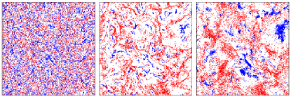
Figure 1: Slice 400$\eta\times$400$\eta\times$10$\eta$ of heavy $\beta\!\!=\!\!0$ (red) and light $\beta\!\!=\!\!3$ (blue) particle positions. From left to right $St\!=\!\ 0.1,1,4.1$. Data refer to the simulation at $\mathrm{Re}_{\lambda}\!=\!180$.

To demonstrate our method, we consider a model of passively advected dilute (to neglect collisions) suspensions of particles in homogeneous, isotropic turbulence. Particles are described as material points which are displaced both by inertial forces (pressure-gradient force, added mass) and viscous forces (Stokes drag). Additional physical effects - as lift force, history force, buoyancy or finite-size and finite-Reynolds corrections - which may becomes important for the cases of light and/or large particles ($\beta St\geq 1$), are here neglected for simplicity.

The particle dynamics then reads Maxey and Riley (1983); Auton et al. (1988) (see also Babiano et al. (2000))

$${\rm d}_{t}\bm{x}=\bm{v}\,,\qquad{\rm d}_{t}\bm{v}=\beta\,{\rm D}_{t}\bm{u}+\tau^{-1}(\bm{u}-\bm{v})\,,$$ (1)

where $\bm{x}\,,\bm{v}$ denote the particle position and velocity, respectively and $d_{t}=\partial_{t}+\bm{v}\cdot\bm{\nabla}$ the time derivative along the particle path. The incompressible fluid velocity $\bm{u}$ evolves according to the Navier-Stokes equations

$${\rm D}_{t}\bm{u}=\partial_{t}\bm{u}+\bm{u}\cdot\bm{\nabla}\bm{u}=-\bm{\nabla}p/\rho_{f}+\nu\Delta\bm{u}+\bm{f}\,,$$ (2)

where $p$ denotes the pressure and $\bm{f}$ an external forcing injecting energy at a rate $\varepsilon=\langle\bm{u}\cdot\bm{f}\rangle$. Eq. (2) is evolved by means of a $2/3$-dealiased pseudospectral code with a second order Adams-Bashforth time integrator. The fluid velocity at particle position is evaluated by means of a three-linear interpolation. Simulations have been performed in a cubic box of side $L\!=\!2\pi$ with periodic boundary conditions, and by using $N^{3}\!=\!128^{3}$ and $512^{3}$ mesh points (reaching Taylor Reynolds numbers $\mathrm{Re}_{\lambda}\!=\!75$ and $180$). The respective Taylor length scales $\lambda\equiv\sqrt{\langle u_{x}^{2}\rangle/\langle\partial_{x}u_{x}^{2}\rangle}$ are $\lambda=13\eta$ and $21\eta$. The parameter space $\beta\times St\!\in\![0\!\!:\!\!3]\times[0\!\!:\!\!4]$ is sampled with $504$ $(\beta,St)$-points with $N=10^{5}$ particles per type in the former case and $64$ (optimally chosen by means of a MonteCarlo allocation scheme based on lower resolution results) with $N=1.6\cdot 10^{6}$ in the latter. Given the small $Re_{\lambda}$ dependence, we will report here mostly results from $\mathrm{Re}_{\lambda}\!=\!75$ as for that case we have a more complete sampling of the parameter space ($\beta,St$).

A requirement for any segregation indicator is to result in zero segregation length for any two statistically independent distributions of particles coming from the same class of particles, at least in the limit of infinitely many particles. If the observation scale is too small and the number of particle finite, even independent particle realizations of the same class of particles will artificially appear to be segregated. Therefore, the definition of segregation strictly requires to indicate the observation scale $r$, and it will be sensitive to the particle number.

However, we aim at a robust observable. Classical and natural observables, as e.g. the minimal distance between different type of particles strongly depends on particle number and hence are not robust. Harmonic averages of particle distances could be sensitive to small scales and not be spoiled by the large scales, but the choice of the weight exponent is rather arbitrary. The use of a density correlation function $\langle\rho_{1}(x)\rho_{2}(x+r)\rangle$ Falkovich et al. (2002), though possible, requires to introduce a coarse-graining scale (to define the densities) which may quantitatively affect the estimate. The mixed pair correlation function, or mixed radial distribution function Zhou et al. (2001), is not bounded at small-scales for clustered distributions of point-particles.

Our approach is inspired by Kolmogorov’s distance measure between two distributions Kolmogorov (1963) and is based on particle densities coarse-grained over a scale $r$, which can be understood as resolution of a magnifying glass used to look at the segregation. The whole volume $L^{3}$ is partitioned into $\mathcal{M}(r)\!=\!(L/r)^{3}$ cubes. We then define the following segregation indicator:

$$S_{\alpha_{1},\alpha_{2}}(r)=\frac{1}{N_{\alpha_{1}}+N_{\alpha_{2}}}\sum^{\mathcal{M}(r)}_{i=1}\left|n_{i}^{\alpha_{1}}-n_{i}^{\alpha_{2}}\right|\,.$$ (3)

The subscripts $\alpha_{1}$ and $\alpha_{2}$ index the particle parameters, i.e., $\alpha_{1}\!=\!(\beta_{1},St_{1})$ and $\alpha_{2}\!=\!(\beta_{2},St_{2})$, $N_{\alpha}$ is the total number of particles of $\alpha$-type, while $n_{i}^{\alpha}$ that of particles contained in each cube $i$. The case $\alpha_{1}\!=\!\alpha_{2}$ should be considered as taking independent realizations of the particle distribution (otherwise $S_{\alpha_{1},\alpha_{1}}\!\equiv\!0$ trivially) so that $S_{\alpha,\alpha}$ sets the minimum detectable segregation degree.

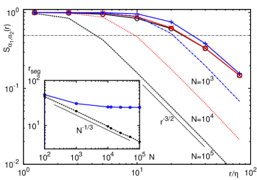
Figure 2: $S_{\alpha_{1},\alpha_{2}}(r)$ vs. $r$ for $\alpha_{1}\!=(\beta_{1}\!=\!0,St_{1}\!=\!1.1)$ (heavy type) and $\alpha_{2}\!=\!(\beta_{2}\!=\!3,St_{2}\!=\!1.1)$ (light type) for different particle numbers $N\;(=\!N_{\alpha_{1}}\!=\!N_{\alpha_{2}})$: $(\circ)$ $N=10^{5}$, $(\times)$ $N=10^{4}$ and $(+)$ $N=10^{3}$. Dashed and dotted lines refer to homogeneously distributed particles samples at various $N$. The expected Poisson scaling behavior, $S_{\alpha_{1},\alpha_{2}}\propto r^{-3/2}$, is also reported. Inset: $r_{seg}$, defined by $S_{\alpha_{1},\alpha_{2}}(r_{seg})=1/2$, as a function of $N$ for both heavy vs. light particles case and Poissonian samples. While for the former $r_{seg}$ saturates as $N$ increases, for the latter $r_{seg}$ goes to zero like $r_{seg,h}\propto N^{-1/3}$, as expected for Possonian samples (see text for details).

Let us first discuss the limiting cases of $S_{\alpha_{1},\alpha_{2}}(r)$. First, it can vary in the range $[0,1]$. $S_{\alpha_{1},\alpha_{2}}(r)=1$ means that the two distributions are not overlapping when looked at resolution $r$. For small enough scales, i.e., $r\ll 1/\rho^{1/3}$ (which is the mean distance of two particles with $\rho=N/L^{3}$ the particle number density) this holds for any realization, therefore $\lim_{r\to 0}S_{\alpha_{1},\alpha_{2}}=1$. On the contrary $\lim_{r\to L}S_{\alpha_{1},\alpha_{2}}=0$ as the total number of particles of the two species is globally identical (as assumed here). These limiting cases are observed in Fig. 2. Clearly, $S_{\alpha_{1},\alpha_{2}}$ is a meaningful indicator of segregation only if it does not depend too severely on the particle number $N$. Indeed, in Figure 2, $S_{\alpha_{1},\alpha_{2}}$ (computed for the red and blue distribution of the central panel of Fig. 1) shows only a very weak $N$-dependence at sufficiently large $N$. This is in contrast with the behavior of (3) for two independent and homogeneously distributed particle realizations (also shown in Fig. 2). The latter case can be easily understood recognizing that in each box of side $r$, $n_{i}$ is a Poisson random variable, so that we can estimate $n_{i}\approx\rho r^{3}\pm\sqrt{\rho r^{3}}$, where the two terms come from the average and the fluctuation contributions, respectively. In eq. (3) the average cancels and, summing the fluctuations over all the $(L/r)^{3}$ cells, one has the order of magnitude estimate $S(r)\sim(L/r)^{3}N^{1/2}(r/L)^{3/2}=N^{1/2}(r/L)^{-3/2}$, explaining both the observed scaling behavior and the strong dependence on $N$.

The segregation indicator allows us to extract the desired segregation length scale $r_{seg}$. This can be done by fixing an arbitrary threshold value for $S$; we employed $S_{\alpha_{1},\alpha_{2}}(r_{seg})=1/2$ (see Fig. 2). With this definition, as shown in the inset of Fig. 2, for truly segregated (heavy vs. light) samples $r_{seg}$ saturates with increasing $N$. This does not hold for uniformly distributed (non-segregated) particles. In the latter case $r_{seg}$ essentially coincides with the interparticle distance $r_{seg}=r_{seg,h}\approx 1/\rho^{1/3}=L/N^{1/3}$, as also seen from the inset of Fig 2. The behavior of $r_{seg}$ encompasses the fact that for a finite number of particles $N$ a natural cut-off distance exists (the mean inter-particle distance) although we know theoretically that $\lim_{N\to\infty}r_{seg}(N)=0$. Hence $r_{seg,h}(N)$ can be interpreted as the accuracy in estimating $r_{seg}$ given a finite particle number $N$.

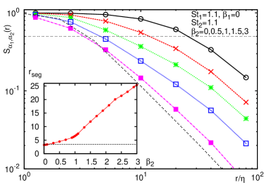
Figure 3: $S_{\alpha_{1},\alpha_{2}}(r)$ for $\alpha_{1}\!=\!(\beta_{1}\!=\!0,St_{1}\!=\!1.1)$ and $\alpha_{2}\!=\!(\beta_{2},St_{2}\!=\!St_{1})$, i.e., a heavy particle with $\beta_{1}=0$ and a given $St$ vs. those having the same $St$ but different densities $\beta_{2}$. From bottom to top: $\beta_{2}=0,0.5,1,1.5,3$. Inset: $r_{seg}$ vs. $\beta_{2}$, with $r_{seg}$ defined as in Fig 2, i.e., $S_{\alpha_{1},\alpha_{2}}(r_{seg})=1/2$. The straight dashed line shows $r_{seg,h}\approx 4\eta\approx 0.3\lambda$.

We now calculate $r_{seg}$ for a pair of two different particle classes to quantify their mutual segregation. Figure  3 displays $S_{\alpha_{1},\alpha_{2}}(r)$ for distributions composed of heavy particles with $\beta_{1}=0$ and $St_{1}=\mathcal{O}(1)$ and particles with the same $St(\!=\!St_{2}\!=\!St_{1})$ but different densities. As one can see, segregation increases with the density difference, but $r_{seg}\approx r_{seg,h}$ for $\beta_{2}<0.5$, meaning that heavy enough particles basically all visit the same locations in the flow, irrespective of their exact density: They tend to avoid vortical regions Bec et al. (2007). A sensitive increase of $r_{seg}$ is observed for $\beta_{2}>1$ (Fig. 3 inset) and as expected the maximal segregation length is obtained for bubbles, i.e., particles with density ratio $\beta=3$, where $r_{seg}\approx 25\eta\approx 1.9\lambda$. For the same case, $St=1.1$, $\beta=0$ vs. $\beta=3$, at $Re_{\lambda}=180$ we find $r_{seg}\approx 29\eta\approx 1.4\lambda$.

Thanks to the large number of particle types in our database we can extend the study of the segregation length to a wide range of physical parameters. In Fig. 4 we show the value of the segregation length by fixing $\alpha_{1}\!=\!(\beta_{1},St_{1})\!=(0,1.1)$ (left), the red particles of central panel of Fig. 1 or the blue ones by fixing $\alpha_{1}\!=(3,1.1)$ (right) and varying $\alpha_{2}\!=\!(\beta_{2},St_{2})$ for the second kind of particles. The emerging picture is as follows. Particle class pairs with $St_{1}\!\approx\!St_{2}$ and $\beta_{1}\!\approx\!\beta_{2}$ have a segregation length close to the interparticle distance $r_{seg,h}$ and are unsegregated, while as soon as the Stokes number or the density difference become larger, $r_{seg}\!>\!r_{seg,h}$. The maximal segregation length ($r_{seg}^{(max)}\!\approx\!27\eta\!\approx\!2.1\lambda$) is roughly twice the Taylor microscale and is realized for particles with large density difference $\beta_{1}=0$ and $\beta_{2}\!>\!1$ (or $\beta_{1}\!=\!3$ and $\beta_{2}\!<\!1$). These results thus confirm those of Fig. 3. It is interesting to note that heavy couples, $\beta_{1},\beta_{2}\!\leq\!1$, segregate less than light ones, $\beta_{1},\beta_{2}\!\geq\!1$, which are thus much more sensitive to small variations of density and/or response times. The correlation between position and flow structure is thus much stronger for light particles.

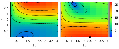
Figure 4: $r_{seg}$ between particle distributions with $\beta\!=\!0$, $St\!=\!1.1$ (left) and $\beta\!=\!3$, $St\!=\!1.1$ (right) vs. distributions with generic $\beta,St$. ($\bullet$) indicates the reference particle type, and ($\times$) the location of the maximal segregation length $r_{seg}^{(max)}$. The solid contour line, traced at $r_{seg}\!=\!r_{seg,h}\!\equiv\!L/N^{1/3}$, sets the sensitivity level to distinguish between segregated and unsegregated particle distributions. Dashed and dotted lines are drawn at $r_{seg}\!=\!n\cdot r_{seg,h}$, with $n=2,\ldots,6$. The color scale codes the value of $r_{seg}$ in units of the Kolmogorov length, $\eta$.

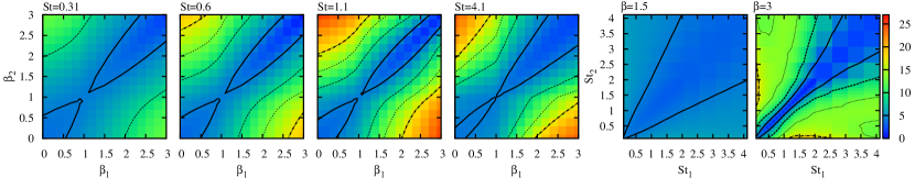
Figure 5: From left to right, segregation length $r_{seg}$ between distribution of particles with $St=(0.31,0.6,1.1,4.1)$ vs. the densities $\beta_{1},\beta_{2}$ and (last two panels) for particle class pairs having the same densities $\beta_{1}=\beta_{2}=1.5$ (resp. $3$) and different $St$. The color scale and the contour lines are, as in Fig. 4, at $r_{seg}\!=\!n\cdot r_{seg,h}$, with $n=2,\ldots,4$.

We next systematically study what happens when fixing $St$ or $\beta$. In the first four panels (from left) of Fig. 5, $r_{seg}$ is shown as a function of $\beta_{1}$ and $\beta_{2}$, where we fixed the Stokes numbers, $St_{1}\!=\!St_{2}\!=\!St\!=\!(0.31,0.6,1.1,4.1)$. Close to the diagonal $\beta_{1}\approx\beta_{2}$ it is $r_{seg}\leq r_{seg,h}$, i.e., similar particles are poorly segregated. Outside these regions $r_{seg}>r_{seg,h}$ and segregation is above the accuracy threshold $r_{seg,h}$. Two observations are in order. First, the strongest segregation is present for the case of $St\!\sim\!1$ meaning that response times of the order of the Kolmogorov time are best suited to generate strong correlations between flow structures and particle positions and consequently segregation. Further, segregation is stronger for couples composed by very heavy ( $\beta\sim 0$) and very light ($\beta\sim 3$) particles. Therefore, light and heavy particles with $St\sim 1$ display the strongest clusterization. Second, the numerical value of the segregation length saturates to a constant value $\approx 2\lambda$, strongly indicating that we are measuring an intrinsic property of the underlying turbulent flow emerging when particles are strongly clusterized.

The two rightmost panels of Fig. 5 display cuts done by fixing the density, namely $\beta_{1}\!=\!\beta_{2}\!=\!\beta\!=\!1.5$ (resp. =3). For $\beta\!<\!1.5$, i.e. relatively heavy or weakly light particles, there is only a slight tendency toward segregation at varying the Stokes number. This means that even if the particles form clusters, such clusters are not too sensitive against variation of $St$. For very light particles, $\beta\!=\!3$, the situation is different when comparing the case of $St\!\sim\!1$ with a $St\sim 0$ case. As expected for $St\!\sim\!0$, though particles are light, they distribute almost uniformly (they are not too far from the tracer limit) while for $St\!\geq\!1$ they are strongly correlated with the vortex filaments which are unevenly distributed in the flow Jimenez and Wray (1998).

In conclusion, we introduced an indicator able to quantify the segregation degree and allowing to define a segregation length scale $r_{seg}$ between different classes of particles, which follow simplified dynamical equations in isotropic turbulence. The extracted information is in line with the intuitive idea of expulsion/entrapment of particles due to vortical structures which is now on a more quantitative ground. The maximal segregation length, for instance for heavy particles ($\beta\!=\!0$, $St\!=\!1.1$), is obtained with bubbles with slightly larger Stokes ($St\!\sim\!1.4$) (Fig. 4 left); it measure $r_{seg}^{(max)}\simeq\!27\eta\simeq\!2.1\lambda$ at $Re_{\lambda}\!=\!75$. At $Re_{\lambda}=180$ we get similarly: $r_{seg}^{(max)}\simeq\!48\eta\!\simeq\!2.3\lambda$. Therefore, $r_{seg}^{(max)}$ is about twice the Taylor length.

Important areas of application of the developed methods go far beyond homogeneous isotropic turbulence including, e.g., heterogeneous catalysis or flotation, where one is interested in the collision probability of argon bubbles and solid contaminations in turbulent liquid steel zha00 . In this context our finding that $r_{seg}^{(max)}\simeq 2\lambda$ suggests that the cleaning could become less efficient at high $Re_{\lambda}$, as bubbles and particles then become more segregated. Hoever, quantitative statement requires better models for both the flow geometry and the effective particle force. Another example for the application of the suggested method is the formation of rain drops at solid nuclei in clouds Falkovich et al. (2002), a mechanism which is crucial to develop models for rain initiation Wilkinson et al. (2006). Disregarding particle segregation in all these examples would lead to estimates of the collision rate which could be orders of magnitude off. We have already observed that the point-particle model adopted in our study neglects some hydro-dynamical effects which corresponds to additional forces in the particle equation. Such forces, when included with proper modeling, might smooth the intensity of segregation which, as we have shown, is mainly due to the relative strength of inertial forces.

Finally, we stress that the introduced segregation indicator can be employed in all phenomena involving different classes of segregating objects. Provided one knows the position of all the objects, no prior knowledge on the physical mechanism which leads to segregation is needed.

We thank J. Bec and L. Biferale for fruitful discussions and R. Pasmanter for prompting Kolmogorov’s distance measure to our attention. Simulations were performed at CASPUR (Roma, IT) under the Supercomputing grant (2006) and at SARA (Amsterdam, NL). Unprocessed data of this study are publicly available at the iCFDdatabase dat .

References

- Maxey (1987) M. Maxey, J. Fluid Mech. 174, 441 (1987).
- Crisanti et al. (1992) A. Crisanti et al., Phys. Fluids A 4, 1805 (1992).
- Balkovsky et al. (2001) E. Balkovsky et al., Phys. Rev. Lett. 86, 2790 (2001).
- Eaton and Fessler (1994) J. Eaton, and J. Fessler, Int. J. Multiph. Flow 20, 169 (1994).
- Bec et al. (2005) J. Bec et al., Phys. Fluids 17, 073301 (2005).
- Wilkinson et al. (2006) M. Wilkinson et al., Phys. Rev. Lett. 97, 048501 (2006).
- Ayyalasomayajula et al. (2006) S. Ayyalasomayajula et al., Phys. Rev. Lett. 97, 144507 (2006).
- Bec et al. (2007) J. Bec et al., Phys. Rev. Lett. 98, 084502 (2007).
- Mazzitelli et al. (2003) I. Mazzitelli et al., J. Fluid Mech. 488, 283 (2003).
- Bec (2003a) J. Bec, Phys. Fluids 15, L81 (2003a).
- Calzavarini et al. (2008) E. Calzavarini et al., J. Fluid Mech. 607, 13 (2008).
- van den Berg et al. (2005) T. H. van den Berg et al., Phys. Rev. Lett. 94, 044501 (2005).
- Rensen et al. (2005) J. Rensen et al., J. Fluid Mech. 538, 153 (2005).
- Ackerman et al. (2004) A. Ackerman et al., Nature 432, 962 (2004).
- Reigada et al. (2003) R. Reigada et al., Proc. Royal Soc. Lond. B 270, 875 (2003).
- (16) L. F. Zhang, and S. Taniguchi, Int. Mat. Rev. 45, 59-82 (2000).
- Falkovich et al. (2002) G. Falkovich et al., Nature 419, 151 (2002).
- Maxey and Riley (1983) M. Maxey and J. Riley, Phys. Fluids 26, 883 (1983).
- Auton et al. (1988) T. Auton et al., J. Fluid Mech. 197, 241 (1988).
- Babiano et al. (2000) A. Babiano et al., Phys. Rev. Lett. 84, 5764 (2000).
- Kolmogorov (1963) A. N. Kolmogorov, Sankhya, A 25, 159-179 (1963).
- Jimenez and Wray (1998) J. Jimenez, and A. A. Wray, J. Fluid Mech. 373, 255–285 (2000).
- Zhou et al. (2001) Y. Zhou, et al., J. Fluid Mech. 433, 77–104 (2001).
- (24) http://cfd.cineca.it