Electronic structure of noble metal impurities in semiconductors: Cu in GaP

Abstract

A numerical method for calculation of the electronic structure of transition metal impurities in semiconductors based on the Green function technique is developed. The electronic structure of 3$d$ impurity is calculated within the LDA+U version of density functional method, whereas the host electron Green function is calculated by using the linearized augmented plane wave expansion. The method is applied to the Cu impurity in GaP. The results of calculations are compared with those obtained within the supercell LDA procedure. It is shown that in the Green function approach Cu impurity has an unfilled 3d shell. This result paves a way to explanation of the magnetic order in dilute Ga_1-xCu_xP alloys.

I Introduction

The experimental and theoretical studies of dilute magnetic semiconductors (see, e.g. the recent review McD ) have revived the interest to details of reconstruction of the electronic structure of host materials induced by transition metal ions and concomitant defects. This interest stems from the fact that the simple Vonsovskii-Zener model of $s$-$d$ exchange is apparently not sufficient for an exhaustive explanation of the behavior of the most popular system (Ga,Mn)As,Bouz1 not to mention the wide-gap materials like (Ga,Mn)N, (Zn,Co)O, (Ti,Co)O₂.Stras ; Coey ; Grif Not only the localized spin of magnetic ions but also the acceptor or donor-like states in the energy gap related to these ions are involved in the indirect exchange between the magnetic ions responsible for the long-range magnetic order. The nature of these states is the matter of a vivid discussion in the current literature.

In particular, an isolated Mn impurity in GaAs creates a 0.11 eV acceptor level relative to the top of valence band. Besides, the electrons in the half-filled $3d$ shell form resonance levels in the middle of this band because of an anomalous stability of the half-filled 3d⁵ shell.Zung86a ; KF94 Since the substitution impurity Mn${}^{2+}(3d^{5})$ is negatively charged relative to the host semiconductor, localizing a hole makes this defect neutral, and the binding energy of this hole is provided by the combined action of the Coulomb potential, central cell substitution potential, hybridization and, maybe, $s$-$d$ exchange.BhaBe ; Krsta At a high enough Mn concentration, these acceptor levels form an impurity band and eventually merge with the hole states near the top of the valence band (see Ref. merge, for a detailed discussion of the current experimental situation).

According to the available calculations of the electronic spectra of an isolated Cu in GaP,Zung85 the copper impurity should have a similar electronic structure. Due to the special stability of the filled 3d¹⁰ shell all the 3d levels of the Cu impurity are expected to be occupied in the ground state, and the electrical neutrality of Cu impurity should be ensured by capturing two holes on Cu-related acceptor levels close to the top of the valence band, so that the resulting electron configuration can be denoted as Cu(d${}^{10}\bar{p}^{2}$). Indeed such acceptor states were found in CaP:Cu samples,Ledebo although at that time the nature of these states remained unclear.

Recently, ferromagnetism with a high Curie temperature in $p$-type Cu-doped GaP was detected.Gupta The EPR signal of the Cu²⁺ state indicates that the 3$d$ shells of Cu impurities are unfilled in this material in contradiction to the results of previous numerical calculations. This discrepancy gives us a motivation to revisit the problem.

We present in this paper the results of numerical calculations of the electronic structure of Cu-doped GaP. Two different computation schemes are used, which give mutually complementary information about the behavior of weakly and strongly doped materials. The first one is the conventional local density approximation (LDA) scheme applied to the lattice of Cu_xGa_1-xP supercells. Similar methods were used for Mn_xGa_1-xPn materials with Pn=As,N,P.Shik ; Kronik The second method is based on the local Green function approach.FK86 In this method the hybridization between the local impurity $d$-orbitals and Bloch waves in the host semiconductor is calculated exactly, without any kind of artificial periodic boundary conditions, and approximations are made only when taking into account the short-range part of substitution impurity potential.

II Green function approach for isolated impurity

A Green function calculation procedure based on the microscopic Anderson model And61 was proposed three decades ago Fleurov1 ; Haldane and later on summarized in Ref. KF94, . This procedure deals with the local Green function

$$G_{\rm imp}({\bf r,r^{\prime}},z)=\sum_{\lambda}|\lambda\rangle\langle\lambda|(z-H)^{-1}|\lambda\rangle\langle\lambda|~{}.$$ (1)

The set $|\lambda\rangle$ includes both the electron states $\phi^{\sigma}_{i_{a}}(\bf r)$ of the electrons localized in the d-shell of impurity atom and the states $\psi_{b,\gamma\mu\sigma}(\bf r)$, which stand for ”the Bloch tail” of the impurity wave function. These states describe the distortion inserted by a substitution impurity in the spectrum of a host crystal. They are superpositions of the Bloch waves, $\psi_{b,\gamma\mu\sigma}=\sum_{{\bf k}n}C^{\gamma\mu}_{{\bf k}n}\psi_{{\bf k}n\sigma}$, where ${\bf k}$ and $n$ are the wave vector and the band index respectively, $\sigma$ is the spin quantum number. Here $\gamma$ is the index of the irreducible representation of the point group characterizing the symmetry of impurity and its surrounding, and $\mu$ denotes its row. Therefore the function $G_{\rm imp}$ is diagonal in $\gamma\mu$ representation. The full Hamiltonian $H$ includes the kinetic and potential energies of all electrons in the impurity atom and in the host crystal, as well as the Coulomb and exchange interactions between these electrons. The projection procedure (1) is exact in principle, and the poles of the Green function $G_{\rm imp}$ describe both continuous and localized impurity related states in the doped crystal. In the practical realization of this method some approximations are unavoidable. The main simplification, which we use here is the approximate treatment of the substitution potential

$$\Delta V({\bf r-R}_{0})=V_{\rm eff}({\bf r-R}_{0})-V_{h}^{0}({\bf r-R}_{0}),$$

where $V_{h}^{0}({\bf r-R}_{0})$ is the potential landscape for an electron in the host gallium atom in the site ${\bf R}_{0}$ and $V_{\rm eff}({\bf r-R}_{0})$ is the self-consistent potential for the electrons in the $3d$ shell of the Cu ion substituting for Ga in this site (see Section III for detailed definition of these potentials). We suppose that this potential is localized within the defect cell of the doped crystal. The ”local substitution potential” approximation influences only the description of $p$-type acceptor states in the lower part of the forbidden energy band. It ignores possible contribution of the Coulomb component of substitution impurity potential. This contribution is known to be small in the case of (Mn,Ga)As,merge and one may hope for a similar situation in (Cu,Ga)P. The principal advantage of the local substitution potential is that in this case the system of Dyson equations for the impurity-related components of the Green function (1) defined as

$$G_{\gamma\mu}(z)=\langle\gamma\mu|(z-H)^{-1}|\gamma\mu\rangle$$ (2)

may be solved analytically FK86 . It yields the equation

$$G^{-1}_{\gamma\mu}(z)=z-\varepsilon_{d\gamma}-{\cal M}_{\gamma}(z)/Q(z),$$ (3)

for the $d$-electron Green function. The positions of electron $d$-levels $\varepsilon_{d\gamma}$ are found self-consistently as a solution of the Schrödinger equation for Cu-related orbitals in the crystalline environment. The self energy in the right-hand side of Eq. (3) contains two contributions. The term ${\cal M}_{\gamma}(z)$ describes the hybridization between the $d$-orbitals and the band electrons

$${\cal M}_{\gamma}(z)=\sum_{n{\bf k}}\frac{|M_{\gamma,n{\bf k}}|^{2}}{z-\varepsilon_{n{\bf k}}}$$ (4)

where the hybridization integral is

$$M_{\gamma,n{\bf k}}=\int\psi^{*}_{d\gamma\mu}({\bf r})\Delta V({\bf r})\psi_{n{\bf k}}({\bf r})d{\bf r}.$$ (5)

The energy bands $\varepsilon_{n{\bf k}}$ and Bloch functions $\psi_{n{\bf k}}({\bf r})$ of the host GaP crystal are calculated by means of the first principle full potential LAPW method MaH ; FaVa (see Section III for details).

The factor

$$Q(z)=1-\Delta V_{0}G_{h}^{0}(z).$$ (6)

in Eq. (3) describes the short-range potential scattering, where

$$\Delta V_{0}=\sum_{n{\bf k}n{\bf k}^{\prime}}\int\psi^{*}_{n{\bf k}}\Delta V({\bf r-R}_{0})\psi_{n{\bf k}^{\prime}}d{\bf r}$$ (7)

is the substitution impurity potential localized in the defect shell,

$$G_{h}^{0}(z)=\sum_{n{\bf k}}\langle n{\bf k}|(z-H_{0})^{-1}|n{\bf k}\rangle=\sum_{n{\bf k}}\frac{1}{z-\varepsilon_{n{\bf k}}}$$ (8)

is the single-site lattice Green function for the electrons in the non-doped host crystal described by the Hamiltonian $H_{0}$.

As was shown in Ref. FK86, , the Green function (3) describes the hybridization between the impurity $d$-electron orbitals and the electrons in the imperfect host crystal, where the band electrons are influenced by the potential scattering $\Delta V$. If this scattering is strong enough, it results in splitting off of localized levels from the top of the valence band. This effect is also taken into account in (3): the positions of the corresponding levels before the hybridization are determined by zeros of the function $Q(z)$ in the energy gap of the host crystal.

One of the fundamental statements of the theory of transition metal impurities in semiconductors Zung86a ; KF94 is the necessity to discriminate between the impurity levels in the gap obtained as solutions of a self-consistent mean-field Schrödinger equation for a doped crystal and the true addition/extraction energy of a $d$-electron to/from the valence/conduction band. The latter energies are determined by the energy balance of ”Allen reactions”Zung86a ; KF94 ; Allen

$$\varepsilon^{n/n-1}=E(d^{n})-E(d^{n-1})-\varepsilon_{v}$$

$$\varepsilon^{n+1/n}=\varepsilon_{c}-E(d^{n+1})+E(d^{n})$$ (9)

Here $E(d^{p})$ is the total energy of doped crystal with the impurity having $p$ electrons in 3d shell. Two Allen reactions describe the electron transition from the top of the valence band $\varepsilon_{v}$ to the empty neutral (acceptor) level and the electron transition from an occupied charged (donor) level to the bottom of the conduction band $\varepsilon_{c}$, so that the energies (II) characterize the true positions of the impurity levels with respect to the band edges in the presence of strong Coulomb and exchange interactions. These energies do not necessarily coincide with the mean-field solutions of the Schrödinger equation due to the violation of Koopmans’ theorem for the impurity ions.

To minimize the mismatch between the single-electron and many-electron states, Slater proposed a concept of ”transition state”. According to his arguments, the ionization energy for a state with $n$ electrons in the 3d shell, $E(d^{n})-E(d^{n-1})$ may be approximated by the energy $\epsilon(n-1/2)$ calculated within the LDA single-electron calculation scheme. More refined LDA+U approach Aza ; Solov takes non-Koopmans’ corrections to the single-electron energies into account explicitly (although still semi-phenomenologically). In terms of the Allen energies (II), the energy $U$ is just the difference between $\varepsilon^{n+1/n}$ and $\varepsilon^{n/n-1}$. We test below both the LDA+U method of Green function calculations and the standard LDA supercell description of dilute (Gu,Ga)P semiconductor.

III Impurity Green functions in LDA+U approximation

To realize a numerical version of the Green function method we use the local density approximation (LDA) and its modification LDA+U, which takes into account strong electron-electron correlations on the impurity site. This section outlines the application of the LDA+U method to systems with local defects with a particular emphasis on the transition metal impurities for which the resonant scattering in the d ($l=2$) channel plays a crucial role. Here we present only the principal features of the scheme leaving many more mathematical details and definitions in Appendix. In this section we retain the spin index, having in mind to use the spin-unrestricted LSDA+U version of this method for the calculation of spin properties of dilute magnetic semiconductors, although in the practical calculations below only the spin-independent LDA+U version is used.

The LDA + U method incorporates a correction to the LDA energy functional which provides an improved description of the electron correlations. The principal idea of the LDA + U method is to separate the electron system into two subsystems of the localized $d$-electrons for which the Coulomb interaction is accounted for by the Hubbard repulsion term $\frac{1}{2}U\sum_{m\neq m^{\prime}}\rho_{m}\rho_{m^{\prime}}$ in the model Hamiltonian whereas the delocalized $s$- and $p$-electrons are described by an orbital independent one electron potential $V^{LDA}({\bf r})$.

As a result the impurity Green function (1) is defined by the Dyson equation

$$G_{i}^{\sigma}(z)=G_{i}^{(0)\sigma}(z)\left[1+{\cal\widetilde{M}}_{i}^{\sigma}(z)G_{i}^{\sigma}(z)\right]$$ (10)

where

$$\widetilde{{\cal M}}_{i}^{\sigma}(z)={\cal M}^{\sigma}_{i}(z)/Q(z).$$ (11)

The Green function (3) is a solution of this equation. We work in the spherically symmetric local basis $(i\equiv plm)$ instead of cubic harmonics expansion $(i\equiv p\gamma\mu)$ used in (3). Here $p$ is the index of repeating irreducible representations $\gamma\mu$ or $lm$, the analog of the principle quantum number $n$ in a spherical atom.

The bare $d$-electron Green function

$$G_{i}^{(0)\sigma}(z)=\frac{1}{z-\varepsilon_{i}-\Delta{V^{\sigma}_{ii}}^{LDA+U}}$$ (12)

includes intraatomic correlations in the form of LDA+U potential consisting of three terms,

$$V\sigma_{ii,\sigma}^{LDA+U}=\Delta V_{ii,\sigma}^{LDA}+\Delta V_{ii,\sigma}^{U}+\Delta V_{ii,\sigma}^{dc}.$$ (13)

Here the first term is the substitution LDA potential

$$\Delta V_{plm,plm;\sigma}^{LDA}=$$

$$\sum_{l^{\prime\prime}}G_{lm,L^{\prime\prime}0}^{lm}\int_{0}^{r_{emb}}drr^{2}\Delta V_{l^{\prime\prime}0,\sigma}^{LDA}(r)R_{pl\sigma}^{2}(r)~{},$$ (14)

The second term is the electron-electron interaction potential in the 3d shell,

$$\Delta V_{ii,\sigma}^{U}=\sum_{m^{\prime\prime}}\left[\left(U_{mmm^{\prime\prime}m^{\prime\prime}}-U_{mm^{\prime\prime}m^{\prime\prime}m}\right)\rho^{-\sigma}_{plm^{\prime\prime},plm^{\prime\prime}}+U_{mmm^{\prime\prime}m^{\prime\prime}}\rho^{\sigma}_{plm^{\prime\prime},plm^{\prime\prime}}\right]$$ (15)

and the last term is the double counting compensation potential, parametrized as

$$\Delta V_{ii,\sigma}^{dc}=-U(\sum_{m\sigma}n_{plm,\sigma}-\frac{1}{2})+J(\sum_{m}n_{plm,\sigma}-\frac{1}{2}).$$ (16)

Here we introduced the occupational matrix

$$\rho^{\sigma,pl}_{mm^{\prime}}=-\frac{1}{\pi}\mbox{Im}\int_{\varepsilon_{b}}^{\varepsilon_{F}}\left[G(z)\right]_{mm^{\prime}}^{\sigma,pl}dz$$

as a contour integral of the relevant matrix elements of the LDA+U Green function (12). The Slater integralsCzy in the atomic limit read

$$U_{m_{1}m_{2}m_{3}m_{4}}\equiv\langle m_{1},m_{3}|V^{ee}|m_{2},m_{4}\rangle$$ (17)

$$=\sum_{k=0}^{2l}a^{k}_{m_{1}m_{2}m_{3}m_{4}}F^{k}(l,l)$$

where the coefficients

$$a^{k}_{m_{1}m_{2}m_{3}m_{4}}=$$

$$\frac{4\pi}{2k+1}\sum_{n=-k}^{k}\langle lm_{1}|Y_{kn}|lm_{2}\rangle\langle lm_{3}|Y^{*}_{kn}|lm_{4}\rangle$$

can be expressed in terms of the Gaunt coefficients $G_{lm,l^{\prime}m^{\prime}}^{l^{\prime\prime}m+m^{\prime}}$ (see Appendix A.3).

The hybridization matrix elements (5) in the numerator of the mass operator now take the form

$$M^{\sigma}_{n{\bf k},i}=$$

$$\int_{\Omega_{emb}}{\phi^{\sigma*}_{i}}({\bf r})\Delta V({\bf r})\Psi^{LAPW}_{n{\bf k}}({\bf r}-\mbox{\boldmath$\tau$}_{s})\Theta({\bf r}-\mbox{\boldmath$\tau$}_{s})d{\bf r}.$$ (18)

Here the Bloch wave functions $\Psi^{LAPW}_{n{\bf k}}$ are calculated by means of the linearized augmented plane wave (LAPW) method, $\mbox{\boldmath$\tau$}_{s}$ is the vector connecting substitution impurity site taken as the point of origin with its nearest P neighbors in the zinc-blend lattice.

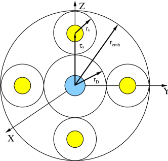
Figure 1: (Color online) The embedded sphere and coordinate system used in our calculations.

In the impurity version of FLAPW method the defect site occupied by a Cu ion is surrounded by the ”embedded sphere” with the radius $r_{\rm emb}$ which includes the impurity sphere with the radius $r_{D}$ (muffin-tin region, where the impurity potential is non-zero). Muffin-tin spheres $r_{s}=(r_{emb}-r_{D})/2$ with a non-zero host lattice potential surround also the neighboring Ga sites (see Fig. 1). The impurity centered basis set is chosen as a set of the linear augmented spherical wave (LASW) functions [see Eqs. (A.1), (24)]. In accordance with the LASW method, a set of Bessel functions is used in the remaining part of the sphere $r_{\rm emb}$. The wave functions in the two regions are matched by the standard boundary conditions imposed on the wave function and its derivative. The Bloch functions $\Psi^{FLAPW}_{n{\bf k}}({\bf r})$ of the host GaP crystal outside the embedded sphere are obtained by the self-consistent FLAPW method. Using the impurity centered local LASW functions we calculate the matrix elements of the host Green function projected onto the local spin polarized LAPW functions in the spherical interstitial site. After matching the boundary conditions (see Appendix), the matrix element (III) is transformed into

$$M^{\sigma}_{n{\bf k},i}=\frac{4\pi\tau_{s}^{2}}{\sqrt{\Omega_{0}}}\sum_{\varrho=1}^{N}v_{n}({\bf k}_{\varrho})\sum_{L^{\prime\prime}M^{\prime\prime}}\sum_{lm}i^{l}Y^{*}_{lm}(\widehat{\bf k}_{\varrho})G^{lm}_{lm-M^{\prime\prime},L^{\prime\prime}M^{\prime\prime}}\int_{0}^{r_{emb}}drr^{2}R_{pl}^{\sigma}(r)\Delta V_{L^{\prime\prime}M^{\prime\prime}}(r){\Phi_{l}^{s}(k_{\varrho},r)}^{LAPW}$$ (19)

($\varrho$ stands for the vectors of reciprocal lattice, see Appendix). As was mentioned above, substituting Ga for a Cu impurity results also in an appearance of a potential component of the impurity potential, which is taken into account approximately by adopting the Koster-Slater-like single site scattering approximation.FK86 Then in accordance with Eq. (10), one may introduce the modified mass operator ${\cal\widetilde{M}}_{i_{a}}^{\sigma}$ (11), where the zeros of the operator $Q(z)$ (6) determine the impurity states, which arise in the doped crystal due to the potential scattering only.

The scattering amplitude $\Delta V_{0}$ is calculated by substituting the LAPW wave functions ${\Psi_{n^{\prime}{\bf k}^{\prime}}}^{LAPW}({\bf r})$ for the Bloch functions in Eq. (7).

As a result the equation for the deep level energy determined as a pole of the impurity Green function (3) within the framework of the LDA+U technique reads

$$z-\varepsilon_{i}-\Delta V^{LDA+U}_{ii}=\widetilde{{\cal M}}_{i}^{\sigma}(z).$$ (20)

It takes into account the resonance part of the scattering amplitude in the d ($l=2$) channel and its mixing with the potential scattering states arising in the p ($l=1$) channel. FK86

The adspace augmentation adspace is used to represent the Green function (or resolvent) $G(z)$ for the GaP crystal with a Cu impurity in the matrix form, Eq. (21). The impurity augmented Green function is subdivided into two blocks, of which the upper left corner block $G^{0}_{A}(z)$ is constructed using the basis of $i$ orbitals where $i$ refer to the $i$-th state with the energy $\varepsilon_{i}$ of the isolated adatom. The host is represented by the lower right corner block $G_{h}^{0}(z)$.

It is worth emphasizing that such a direct introduction of the new adatom related states is very effective in the matrix formulation. Since the high energy part of the spectrum of the differential operator is well suited for the description of the strongly localized $d$-type impurity states,Lind the issue of the necessary number of the host crystal bands becomes crucially important. The direct introduction of the $d$-states drastically simplifies the problem. The Dyson equation may be then split into two independently solvable equations (see Appendix) which finally allows one to carry out the calculations of the GaP host Green $G^{0}_{h}(z)$ using only 15 bands.

The problem is treated self consistently, starting with the trial set of LAPW functions obtained with the help of the impurity potential, which in the zero’s approximation is just a sum of the atomic potentials of the defect crystal. The self-consistency procedure for $\Delta V({\bf r})$ is carried out in a mixed fashion. The first two iterations use the arithmetic average scheme, which later on is effectively substituted by the Aitken scheme.Aitken Just seven iterations produce the $\approx 2\cdot 10^{-4}$ Ry self-consistency.

The equations presented in this Section will be our working formulas for the LDA+U calculations of the Ga(Cu)P compound where the Cu atoms substituting Ga host atoms will be considered as isolated impurities. A possible exchange interaction between the Cu atoms and the resulting magnetic effects will be considered elsewhere.

IV Discussion of the results

This section presents the results of calculation of the electronic structure of Cu_xGa_1-xP obtained by means of the two methods, both using the LDA approximation. The Green function approach is based on the band structure calculated by means of the FLAPW method discussed in the previous section. The supercell approach uses the AS-LMTO methodWil for the band calculations. The VoskoCap and Perdew-Wang Per parametrization scheme is used for the calculation of the exchange-correlation potential in the former and latter approaches, respectively. Brillouin zone (BZ) integration is performed using the improved tetrahedron method.tet

According to the present FLAPW and LMTO calculations, the undoped GaP is a semiconductor with the 1.83 eV FLAPW indirect gap and 1.61 eV ASA-LMTO gap between the top of the valence band (VB) at the $\Gamma$ point and the bottom of the conduction band (CB) at the (0,0,0.875) point close to the $X$ point of the fcc BZ. A direct gap of 1.77 eV opens at the $\Gamma$ point. The 6.8 eV width valence band is formed by the strongly hybridized P $p$ and Ga $s$ and $p$ states while the states at the top of VB in the vicinity of $\Gamma$ are formed by the P and Ga $p$ states with a dominant contribution of the former. The band originating from the P related $s$ states hybridized with the Ga related $s$ states is found between $-$12.5 and $-$9.5 eV and separated by a gap of 2.8 eV from the bottom of the valence band. The density of states (DOS) of GaP is visualized in Fig. 2 as the imaginary part of the Green function $G^{0}_{h}$ (8) calculated by the LAPW method.

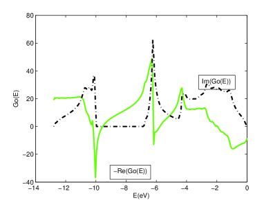
Figure 2: (Color online)The functions Re$(G_{h}^{0})$ and Im$(G_{h}^{0})$ for GaP.

A similar picture is obtained by direct band structure calculations within the ASA-LMTO method. The difference in the widths of the energy gaps only weakly influences the structure of the Cu-related states in the energy spectrum of doped samples. We start the discussion of these states with a discussion of the supercell calculations.

IV.1 Supercell energy spectrum of ${\rm Cu_{1-x}Ga_{x}P}$

The electronic structure of Cu_xGa_1-xP with $x$ varying from 0.125 down to $\sim$0.016 was calculated using $2a\times 2a\times 2a$, $3a\times 3a\times 3a$, and $4a\times 4a\times 4a$ supercells of the cubic zinc-blend lattice. Calculations for $x$=0.125 (1/8), 0.063 (1/16), and 0.031 (1/32) were performed for $F\overline{4}3m$ (216) fcc, $I\overline{4}3m$ bcc (217), and $P\overline{4}3m$ (215) simple cubic unit cells, respectively. The face-centered cubic cells with $a=3a_{0}$ and $a=4a_{0}$ allowed to simulate compositions with $x\approx 0.037$ (1/27) and $x\approx 0.016$ (1/64). In all the calculations the Ga ion in the (0,0,0) position was substituted by the Cu ion with the same atomic sphere radius. This way the tetrahedral ($T_{d}$) symmetry of the Cu impurity site was preserved. The positions of host atoms around the Cu impurity were not relaxed.

Upon the Cu substitution Cu_xGa_1-xP becomes a metal with each Cu impurity creating 2 holes in the valence band. At all the compositions $x$ studied in the present work the Fermi level ($\varepsilon_{F}$) crosses the three bands which are triply degenerate at the highest energy in the $\Gamma$ point. At $x$=0.063 the top of the valence band lies 0.42 eV above $\varepsilon_{F}$ and moves to 0.13 eV as the Cu concentration decreases to $x$=0.016. As an example, bands calculated along some high symmetry directions for Cu_xGa_1-xP with $x$=0.031 are show in Fig. 3. At this Cu concentration the top of the valence band is situated 0.22 eV above $\varepsilon_{F}$.

Figure 3: (Color online) Bands calculated along some high symmetry directions and the total DOS for Cu_xGa_1-xP with $x$=0.031.

Figure 4 (lower panel) shows the density of Cu $d$ states in Cu_xGa_1-xP with $x$ = 0.031 projected onto the irreducible representations $e$ and $t_{2}$ of the $T_{d}$ symmetry group. The densities of $p$ states of the nearest (P₁ and Ga₁) and next nearest (P₂ and Ga₂) neighbors of the Cu impurity are presented in the middle and upper panels of Fig. 4.

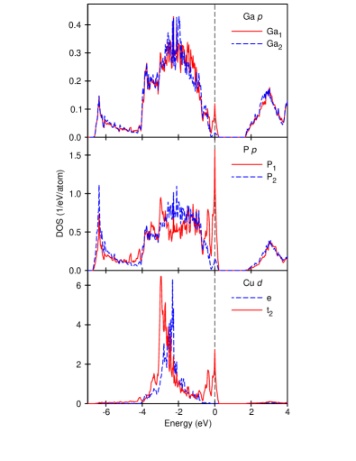
Figure 4: (Color online) A symmetry resolved density of Cu $d$ states (lower panel) and the density of P $p$ (middle panel) and Ga $p$ (upper panel) states calculated for Cu_xGa_1-xP with $x$=0.031.

The calculations show that the Cu $d$ shell is almost completely filled and the Cu valency is close to $1+$. Cu $d$ states of $e$ symmetry ($3z^{2}-1$ and $x^{2}-y^{2}$) form a DOS peak centered at $-$2.5 eV. They are completely occupied and do not contribute to the bands crossing the Fermi level. The main peak of the density of the $t_{2}$ ($xy$, $yz$, and $zx$) states is located at $-3$ eV. However, another two peaks of $t_{2}$ DOS are clearly seen just at $\varepsilon_{F}$ and $0.5$ eV below it. The origin of these peaks becomes more clear when the Cu $t_{2}$ DOS is compared to the density of $p$ states of the P₁ ion closest to Cu. The latter shows two prominent peaks exactly at the same energies. Similar peaks can also be observed in Ga₁ DOS as well as in DOS of the more distant P and Ga ions not shown in Fig. 4. An analysis of the partial occupations shows that of 2 holes ($h$) created by the Cu impurity only 0.18 $h$ is provided by the Cu $t_{2}$ states. Another 0.48 $h$ is distributed over the $p$ states of 4 $P_{1}$ ions whereas the remaining 1.36 $h$ is spread over more distant neighbors.

It is worth noting that in spite of the appearance of the narrow DOS peak exactly at $\varepsilon_{F}$ the spin-polarized calculations failed to produce a ferromagnetic solution even for the highest Cu concentrations studied. Apparently, this can be explained by the delocalized character of the states responsible for the peak and an insufficient strength of the Hund’s exchange coupling for P and Ga $p$ states, which give the dominant contribution to the corresponding bands. At the same time, the contribution of Cu $d$ states, for which a strong on-site exchange interaction is expected, to the peak at $\varepsilon_{F}$ is relatively small.

We also performed test calculations for a few values of $x$ in $E_{x}$Ga_1-xP, in which a Ga ion was substituted by a vacancy $E$. A vacancy creates one more hole in the valence band as compared to Cu. Nevertheless, in the vicinity of the Fermi level the band structures calculated for $E_{x}$Ga_1-xP are similar to those for Cu-doped GaP. In particular, the density of P₁ states at and just below $\varepsilon_{F}$ has the same two-peak shape. These peaks are also reflected in the density of $E$ $d$ states of the $t_{2}$ symmetry, however, they are much less pronounced than the corresponding peaks of Cu $t_{2}$ DOS. Significantly higher peaks can be observed in the density of $E$ $p$ states which also transform according to the $t_{2}$ representation.

Thus, we may conclude that the bands crossing $\varepsilon_{F}$ in Cu_xGa_1-xP are mainly formed by the $p$ states of the nearest to the Cu impurity P₁ ions that split off from the top of the GaP valence band as a result of breaking of the covalent P $p$ – Ga bonds at the impurity site. These states have $t_{2}$ symmetry and hybridize strongly with the corresponding Cu $d$ states. These states are, however, rather extended, which leads to a relatively strong dispersion of the split-off bands even for $x$=0.016.

IV.2 Cu-related energy states of isolated impurity

Before turning to the calculation of the Cu-impurity related levels in the host GaP, let us look at the energy dependence of the self energy part (4), which is responsible for the renormalization of $3d$ levels due to the hybridization with the host band states. The hybridization matrix elements $M_{n{\bf k},i_{a}}$ are calculated by means of Eq. (III) using the Cu 3$d$ impurity wave functions and LAPW functions of the GaP host. Since the LAPW wave functions are defined within the volume subdivided into two muffin-tin parts and the surrounding volume, the integration in Eq. (III) is carried out in all three parts separately accounting for all the hybridization contributions as well as for the covalency induced non-spherical components of the difference potential.

Figure 5 represents the real and imaginary parts of ${\cal M}_{i}(\varepsilon)$ obtained for the (Ga,Cu)P compound. Here index $i$ represents one of the components of the $t_{2}$ irreducible representation. Comparison of ${\rm Im}{\cal M}_{t_{2}}(\varepsilon)$ with the density of band states which is shown as ${\rm Im}(G_{h}^{0})$ in Fig. 2 demonstrates that the weighting of the density of states with the squared hybridization matrix element reproduces the general shape and van Hove singularities of the partial $p$-component of DOS. The differences between ${\rm Re}(G_{h}^{0})$ and ${\rm Re}{\cal M}_{t_{2}}(\varepsilon)$ are more noticeable. Both these functions are sums of the Hilbert transforms of the DOS and weighted DOS for all the valence and conduction bands, respectively. Therefore these function not only map the singularities of DOS in the given band on the singularities of its Hilbert transform but also accumulate asymptotic contributions of higher and lower bands at the given $\varepsilon$. This accumulation results in a noticeable smoothing of the ${\cal M}_{t_{2}}(\varepsilon)$ function in the $-6$ to 0 eV range. Besides, weighting with $M^{2}_{t_{2}}(\varepsilon)$ strongly reduces the amplitude of ${\rm Re}{\cal M}_{t_{2}}(\varepsilon)$ in comparison with ${\rm Re}(G_{h}^{0})$. Such strong reduction means that the hybridization-induced renormalization of the atomic $3d$ levels of the isolated Cu impurity is small enough, and their positions are predetermined mainly by the impurity core potential and Coulomb interaction within the muffin-tin sphere $r_{D}$.

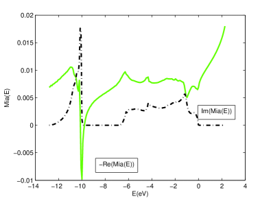
Figure 5: (Color online)Real and imaginary parts of mass operator ${\cal M}_{i_{a}}(\varepsilon)$ for (Ga,Cu)P.

To compare the energy spectrum of the Cu impurity in GaP obtained by the Green function method with that given by LDA in the supercell calculation scheme, we first compute this spectrum by solving Eq. (20) within the LDA scheme without the second term $\Delta V_{ii}^{U}$ in the impurity potential (13). Both the resonant and short range potential components of impurity scattering were taken into account. These calculations yield the value $\varepsilon_{v}-0.66$ eV for the impurity $d_{t_{2}}$ resonance in the valence band, which is higher than that in the supercell calculation, and the $d_{e}$ peak lies slightly above this level. Apparently, these peaks are related to the van Hove singularities in the heavy hole band. These resonances are shallower than those seen in the supercell DOS (Fig. 4). As was mentioned above, the $d_{e}$ peak in the latter structure is located at $\varepsilon_{v}-2.5$ eV. However, one should remember that the center of gravity of the valence band DOS is shifted downward with respect to its position in the pure GaP due to the transformation of $d_{e}$ and $d_{t_{2}}$ levels into $d$-bands (see Fig. 3). Potential scattering built in the self energy part $\widetilde{M}_{i}(z)$ in Eq. (20) results in the appearance of an empty impurity level at $\varepsilon_{v}+0.168$ eV. This acceptor level may be identified with the $x\to 0$ limit for the P related $p$-structure at the top of the valence band in the supercell DOS (Fig. 4, middle panel). The occupation of the impurity $d$-shell in this case is close to 10, like in the supercell calculations.

The computation of the impurity spectrum within the LDA+U scheme yields a self-consistent solution for the electron spectrum only for the transition state 3d^8.5 of Cu impurity. This solution is described below. First, we determined the position of non-perturbed 3d-level of the Cu atom and the correlation parameters $U-J$. The isolated impurity energy $\varepsilon_{i}(+8.5)=-20.9$ eV is calculated by means of the semi-relativistic RATOM programatom for the 3d^8.5 configuration, which corresponds to the concept of the transition state adopted in this paper. The intraatomic Coulomb repulsion of the $d$-electrons is treated in the LDA + U approximation and $m$-dependent Coulomb integrals (17) are calculated. The choice of the parameters $U=4.5$ eV and $J=0.7$ eV is based on the analysis of the occupation numbers in the transition state approach.Sato The self-consistent single electron 3$d$-level for the embedded Cu impurity in the 3d^8.5 configuration is in resonance with the valence band of GaP host crystal, and the impurity-related resonance and discrete states are found as solutions of Eq. (20).

Figure 6: Electronic structure of (Ga,Cu)P, calculated from Eq. (20). The lowest of the five levels in the left panel correspond to the states $(2,\pm 1)$, the next $(l,m)$ levels are classified as (2,-2),(2,0) and (2,+2) (bottom-up). See the text for further discussion

Figure 6 depicts the electronic structure of (Ga,Cu)P calculated by the Green function method. We present here three versions of the calculations which account for: (a) resonant scattering, (b) short range potential scattering, and (c) combined case.

In the resonant scattering approximation (Fig. 6a) where the term $Q^{-1}(z)$ is omitted in Eq. (20), there are four occupied levels in the valence band and one empty level in the energy gap. The occupied states correspond to the configuration Cu($d^{8})$ of the impurity ion. These levels reflect the multiplet structure of this configuration. Although we used the orbital quantum numbers in our computation procedure, the calculated electron density distribution reveals the $T_{d}$ point symmetry of the impurity surrounding. In terms of the corresponding cubic harmonics the lowest state has the $t_{2}$ symmetry, the two next levels belong to the $e$-representation, and the empty state in the energy gap is the $t_{2}$ state of the configuration $d^{9}$. In terms of the Allen diagrams (II) these levels correspond to the addition energy $\varepsilon_{t_{2}}^{9/8}=E(e^{4}t_{2}^{5})-E(e^{4}t_{2}^{4})$ and $\varepsilon_{e}^{9/8}=E(e^{4}t_{2}^{5})-E(e^{3}t_{2}^{5})$ for $d_{t_{2}}$ and $d_{e}$ quantum numbers, respectively (see similar classification for (Ga,Ni)P in Ref. Zung85, ). The final $3d^{8}$ states belong to the ${}^{3}T_{2}(F)$ and ${}^{3}T_{1}(F)$ representations in the Tanabe-Sugano classification.Zung86a ; KF94 ; FK86 ; Zung85

The energy interval between the multiplet of occupied levels in the valence band and the empty level in the energy gap is $\lesssim 4$eV, which is comparable with the value of the input parameter $U-J=3.8$ eV. The hybridization renormalization due to the self energy ${\cal M}(z)$ in Eq. (20) is 0.115 eV for the occupied levels and 0.182 eV for the empty level. In the calculation procedure described above, the difference in hybridization shifts for $t_{2}$ and $e$-levels was neglected, because the hybridization (ligand field) contribution is small enough for the Cu impurity ion.

Figure 6b exhibits the net contribution of potential scattering (III) to the formation of impurity-related states. The levels shown in this figure are obtained from (20) with ${\widetilde{\cal M}}$ substituted for $Q^{-1}$ [see Eq. (11)]. The states in the occupied part of the spectrum are the impurity resonances in the valence bands around the maxima of the partial $p$-wave contributions at the energies $\sim-6$eV and $\sim-2$eV (cf. Figs. 4 and 5). The $p$-level arises at the energy $+0.68$eV above the top of the valence band.

Both the $d$- and $p$-like states are found in the solution of Eq. (20) with the full self energy ${\widetilde{\cal M}}$ (Fig. 5c). The most significant difference between the combined spectrum of Fig. 5c and those of Fig. 5a,b is the noticeable hybridization between $p$ and $d_{t_{2}}$ resonances in the valence band, whereas thee $d_{e}$ levels are only slightly shifted. The shallow $p$-level in the energy gap is pinned to its original position shown in Fig. 5b, in spite of $dp$ hybridization. All these results agree with qualitative predictions of the analytical model taking into account both resonant and short-range potential stattering.FK86

There is no straightforward way to compare the results of LDA+U calculations with those obtained within the LDA scheme, since the former method uses the fitting parameters $U,\ J$, whereas the latter one is based on the variational approach, which formally gives the solution corresponding to the minimal total energy. We only may estimate the total energies of the two solutions by comparing the positions of the impurity levels obtained by both methods within the same Green function approach. LDA procedure gives the occupied $e$ and $t_{2}$ levels at the energies $\sim\varepsilon_{v}-0.64$ to 0.66 eV below the top of the valence band and the shallow $p$-level at the energy $\varepsilon_{v}+0.168$ eV, which corresponds to the configuration $d^{10}\bar{p}^{2}$: two holes neutralize the excess charge in the $d$ shell, which means that the triply degenerate $p$-level is occupied by one electron. In the LDA+U solution the occupied $t_{2}$ and $e$-levels lie essentially deeper in the valence band at the energies $\sim\varepsilon_{v}-2.3$ to 1.8 eV, Cu ion behaves as the isoelectronic impurity ${\rm Cu}^{3+}(d^{8})$, and the acceptor $p$-levels are triply occupied in the neutral impurity state. The comparison of single-electron energies for the two solutions gives the energy gain $\sim 10.7$ eV for the latter state. It is hardly probable that the exchange-correlation contribution may change the energy balance in favor of a state with the fully occupied 3$d$ shell of the Cu impurity.

Comparing the electronic structures of (Ga,Cu)P obtained by the supercell and Green function methods, one may indicate both similarities and dissimilarities in the description of impurity-related states.

First, both methods provide the same mechanism for formation of the shallow $p$-levels in the energy gap of the host material, which merge into the impurity band at a high enough dopant concentration. These levels are split off from the top of the valence band and partially hybridized with the $t_{2}$ levels in the valence band.

Second, the spectral density of the impurity related $d_{\gamma}$-states is concentrated mainly in the valence band with the $d_{t_{2}}$ component lying below the $d_{e}$ component. Here, however, the important difference between the two approaches should be emphasized. As was mentioned above, the $d_{\gamma}$ resonances calculated within the Green function LDA approximation are shallower than those found by means of the supercell approach. One may see also a difference in the $d_{e}-d_{t_{2}}$ splitting: it can be estimated as $\sim 0.5$eV in the supercell calculations and as $\lesssim 0.3$eV in the Green function calculations. The main reason of this difference is the fact that the impurity $3d$-levels are transformed in an effective $d$-bands in the periodic supercell structure, and the hybridization repulsion between the two Bloch waves is stronger than that between the localized $d$-levels and periodic partial $p$-waves in the Green function approach. The same argument is valid for the quasiband method used in the calculations of Ref. Zung85, , where the Cu-related $d$ - levels are located even deeper than in our supercell calculations at the energies $\sim 3-4.5$ eV below the top of the valence band of GaP.

The most important difference between the results described in Subsections IVA and IVB is of course the difference in the electron configuration of Cu impurity, which is $d^{10}\bar{p}^{2}$ in the supercell calculations and $d^{8}$ in the Green function calculations. Available experimental data Gupta are in favor of the configuration $d^{9}\bar{p}$. At this stage we have no exhaustive explanation of these discrepancies. First, our scheme should be extended to the spin-unrestricted LSDA solution and to the multiimpurity case. We expect that the charge configuration of Cu ions is highly sensitive both to the spin state and to the interimpurity coupling. Second, more experimental investigations are necessary, which would reveal the role of concomitant defects, the annealing conditions, the thickness of the film and other technological factors. It is also worthwhile checking whether the use of LDA+U method in the supercell approach may result in the configuration with an incomplete $3d$ shell of the Cu impurity. We leave all these questions for further investigations.

V Concluding remarks

The numerical solution of the Dyson equation (20) derived by means of the Green function method reveals similarities and dissimilarities between the electronic structures of the Mn impurity (half-filled 3$d$ shell in atomic state) and Cu impurity (completely filled 3d shell in atomic state) substituting for Ga in zinc blende semiconductor. Our calculations show that unlike Mn, which retains its stable half-filled 3d⁵ shell in the host GaAs and GaP crystals,McD ; merge the Cu impurity may release some of its $d$-electrons from the stable filled shell 3d¹⁰ to minimize the total energy of doped crystal, at least in the wide-gap GaP. Our theoretical result partially agrees with the experimental observation of Cu ions with unfilled 3d shell in GaP.Gupta It paves a way to theoretical explanation of the ferromagnetic ordering in Ga_1-xCu_xP crystals, although for this purpose further development of the Green function method is necessary. The results of the numerical study of magnetic ordering by means of the Green function method will be published elsewhere.

This work is partially supported by the Max-Planck Gesellschaft during the stay of O.F., K.K. and V.F. in MPIPKS (Dresden), where this work was completed.

Appendix A Details of computational scheme

In order to realize the GF approach in a computational scheme we make use of the local density approach (LDA)Far and its LDA+U modification Anis93 which accounts for a strong electron-electron interaction. The approximation Cap is used for the exchange-correlation potential. The band structure of the GaP semiconductor is calculated by means of the ab-initio full potential all electrons LAPW method.FaVa This method presents the charge density and the crystal potential as a series of the spherical harmonics inside the muffin-tin spheres and of the plane waves outside the spheres. The self-consistent electronic band structure is determined by solving a single particle Dirac equation by using the variational method in LAPW - function basis {$\Psi^{LAPW}_{n{\bf k}}({\bf r})$}. In order to evaluate the Coulomb part of the crystal potential we use the concept of multipole potentials and solve the Dirichlet problem for the sphere with all the contributions being treated on equal footing.FaVa The exchange-correlation potential is approximated by the Padé approximant technique in order to interpolate accurately the recent Monte Carlo results with the RPA spin-dependent data.Cap The Fourier components of the exchange - correlation potential in the interstitial region are fitted in the least square method by applying the singular value decomposition procedure. The charge density in the interstitial region is calculated in ca. 2000 to 3000 random points in the irreducible wedge of the Wigner-Seitz cell.

In order to find the self energy ${\cal M}_{i}(z)$, one has to calculate the matrix elements $M_{n{\bf k},i}$ between the band states $|n{\bf k}\rangle$ and the states $|i\rangle\equiv|plm\rangle$ of the impurity atom. A computational scheme based on the augmented Green functionsKZ

$${\sf{G}}^{0}(z)=\left(\begin{array}[]{cc}G^{0}_{A}(z)&0\\ &\\ 0&G^{0}_{h}(z)\end{array}\right)$$ (21)

is developed for this sake. Here

$$G^{0}_{A}({\bf r},{\bf r}^{\prime};z)=\sum_{i=p,l,m}\frac{\phi_{i}({\bf r})\phi^{*}_{i}({\bf r})}{z-\varepsilon_{i}}$$

is the impurity Green function, whereas the host crystal is represented by

$$G_{h}^{0}({\bf r},{\bf r}^{\prime};z)=\sum_{n=1}^{P}\sum_{{\bf k}\in IBZ}\frac{\Psi^{LAPW}_{n{\bf k}}({\bf r}){\Psi^{LAPW}_{n{\bf k}}}^{*}({\bf r}^{\prime})}{z-\varepsilon_{n{\bf k}}}.$$

The wave functions of electrons localized in the impurity 3$d$ shell are defined within the impurity sphere $r\leq r_{D}$ (see Fig. 1): $\phi_{plm}({\bf r})=R_{pl}(r)Y_{lm}(\widehat{{\bf r}})$. The radial parts of these functions are defined as solutions of the equation

$$\left[-\nabla^{2}+V_{h}^{0}(r)+\Delta V(r)\right]R_{pl}(r)=\varepsilon_{pl}R_{pl}(r),$$ (22)

and the angular parts are represented by the spherical harmonics. The Bloch wave functions are expanded in the reciprocal wave vectors ${\bf k}_{\varrho}={\bf k}+{\cal K}_{\varrho}$

$$\Psi^{LAPW}_{n{\bf k}}({\bf r})=\sum_{\varrho=1}^{N}v_{n}({\bf k}_{\varrho})\varphi_{{\bf k}_{\varrho}}({\bf r})$$

where

$$\varphi_{{\bf k}_{\varrho}}({\bf r})=\frac{1}{\sqrt{\Omega_{0}}}\left[e^{i{\bf k}_{\varrho}{\bf r}}\Theta_{int}({\bf r})+\sum_{s}\Theta_{s}(\mbox{\boldmath$\rho$})e^{i{\bf k}_{\varrho}{\mbox{\boldmath$\tau$}}_{s}}4\pi r_{s}^{2}\sum_{lm}i^{l}\Phi^{(s)}_{lm}({\bf k}_{\varrho},\mbox{\boldmath$\rho$})Y^{*}_{lm}(\widehat{k}_{\varrho})\right]$$

with

$$\Phi^{(s)}_{lm}({\bf k}_{\varrho},\mbox{\boldmath$\rho$})=$$

$$\left[a_{l}^{(s)}({\bf k}_{\varrho}){\cal{R}}^{(s)}_{l}(\varepsilon_{l},\rho)+b_{l}^{(s)}({\bf k}_{\varrho})\dot{{\cal{R}}}^{(s)}_{l}(\varepsilon_{l},\rho)\right]Y_{lm}(\widehat{\mbox{\boldmath$\rho$}}).$$

The following notations has been used above:

$$\Theta_{int}({\bf r})=\left\{\begin{array}[]{ll}1,&{\bf r}\in\Omega_{int}\ -\ \mbox{volume of the}\\ &\ \mbox{interstitial region}\\ &\\ 0,&\ \mbox{otherwise},\end{array}\right.$$

$$\Theta_{s}(\mbox{\boldmath$\rho$})=\Theta_{s}({\bf r}-{\mbox{\boldmath$\tau$}}_{s})=\left\{\begin{array}[]{ll}1,&{\boldmath\rho}\in\Omega_{s}\ -\ \mbox{volume of the}\\ &\mbox{$s$ sphere region}\\ &\\ 0,&\ \mbox{otherwise},\end{array}\right.$$

$v_{n}({\bf k}_{\varrho})$ are eigenvectors of LAPW variation procedure; $n$ is the number of the accounted energy bands, $\Omega_{0}$ is the volume of the Wigner-Seitz cell, $a_{l}^{(s)}({\bf k}_{\varrho})$ and $b_{l}^{(s)}({\bf k}_{\varrho})$ are the muffin-tin coefficients in the LAPW method, and $\dot{{\cal{R}}}^{(s)}_{l}(\varepsilon_{l},\rho)=\frac{\partial}{\partial\varepsilon}{{\cal{R}}}^{(s)}_{l}(\varepsilon,\rho)|_{\varepsilon_{l}}$ for the fixed energy $\varepsilon_{l}$. ${\cal{R}}^{(s)}_{l}(\varepsilon_{l},\rho)$ is the radial part of the LAPW function.

A.1 Choice of the localized basis

Calculations of the electronic structure of defects in crystals are usually based on the pseudopotential or LCAO + pseudopotential approachBernholc ; Baraff . This method requires a large number of the Gaussian orbitals and calculation of their overlap integrals. Instead we perform here an all-electron calculation which allows one to realize the spin-polarization LDA + U scheme. This approach uses the basic set of $N_{D}$ functions

$$\chi_{\mu}({\bf r})\equiv\chi_{pLM}(r,\vartheta,\varphi)=$$

$$\left\{\begin{array}[]{cc}F_{{\bf p}L}(r)Y_{LM}(\hat{\bf r}),&\mbox{for}\ r\leq r_{D},\\ &\\ j_{L}(\kappa_{{\bf p}L}r)Y_{LM}(\hat{\bf r})&\mbox{for}\ r>r_{D}\end{array}\right.$$ (23)

Here $L$ is a non-negative quantum number and $-L\leq M\leq L$, the inverse length $\kappa_{pL}$ is defined by zeros of the Bessel function $j_{L}(\kappa_{L_{p}}r_{emb})=0$ for the radius $r_{emb}$ of the embedded sphere; $p$ is the integer number enumerating these zeros. The radial part of the wave function (A.1) is

$$F_{pL}(r)=a_{L}(\kappa_{pL})R_{L}(\varepsilon_{L},r)+b_{L}(\kappa_{pL})\dot{R}_{L}(\varepsilon_{L},r).$$ (24)

Here the parameters

$$a_{L}(\kappa_{pL})=\frac{\dot{R}_{L}j_{L}^{\prime}(\kappa_{pL}r_{D})-{\dot{R}_{L}}^{\prime}j_{L}(\kappa_{pL}r_{D})}{\dot{R}_{L}R_{L}^{\prime}-R_{L}\dot{R}_{L}^{\prime}}$$

$$b_{L}(\kappa_{pL})=\frac{R_{L}^{\prime}j_{L}(\kappa_{pL}r_{D})-R_{L}^{\prime}j_{L}^{\prime}(\kappa_{pL}r_{D})}{\dot{R}_{L}R_{L}^{\prime}-R_{L}\dot{R}_{L}^{\prime}}$$

are used to match the function (24) to the Bessel functions outside the muffin-tin region, $R_{L}\equiv R_{L}(\varepsilon_{L},r)$, $R_{L}^{\prime}=\displaystyle\left.\frac{dR_{L}(\varepsilon_{L},r)}{dr}\right|_{r=r_{D}}$, $\displaystyle\left.\dot{R}_{L}=\frac{dR_{L}(\varepsilon_{L},r)}{d\varepsilon_{L}}\right|_{r=r_{D}}$.

The above basis $\chi_{\nu}({\bf r})$ was used in the Cholesky decomposition ${\textsf{S}}={\textsf{L}}\cdot{\textsf{L}}^{\dagger}$ for the overlap matrix

$$S_{\mu\nu}=\int_{\Omega_{emb}}\chi_{\mu}^{*}({\bf r})\chi_{\nu}({\bf r})d{\bf r}$$

in order to obtain the orthonormal basis

$$\widetilde{\chi}_{\mu}({\bf r})=\sum_{\mu^{\prime}}({\textsf{L}}^{-1})^{\dagger}_{\mu\mu^{\prime}}\chi_{\mu^{\prime}}({\bf r}).$$

Then the Green function of the host crystal is projected onto the localized basis

$$G_{h,\mu\nu}^{0}(z)=\sum_{n=1}^{M}\sum_{{\bf k}\in IBZ}\frac{\langle\widetilde{\chi}_{\mu}|\Theta|\Psi^{LAPW}_{n\bf k}\rangle\langle\Psi^{LAPW}_{n\bf k}|\Theta|\widetilde{\chi}_{\nu}\rangle}{z-\varepsilon_{n\bf k}}$$

and calculated by means of the analytical tetrahedron method tet within the irreducible part of the Brillouin zone (IBZ)

$$G_{h,\mu\nu}^{0}(z)=\sum_{n=1}^{M}\sum_{{\bf k}\in IBZ}w_{n\bf k}(z){\cal F}_{n{\bf k},\mu\nu}.$$

Here

$${\cal F}_{n{\bf k},\mu\nu}=\langle\widetilde{\chi}_{\mu}|\Theta|\Psi^{LAPW}_{n{\bf k}}\rangle\langle\Psi^{LAPW}_{n{\bf k}}|\Theta|\widetilde{\chi}_{\mu}\rangle.$$

The coefficients $w_{n\bf k}(z)$ depend only on the dispersion relation $\varepsilon_{n{\bf k}}$ and can be computed only once.

A.2 Self energies for impurity Green function

The impurity Green function (10) contains several self energy corrections to the atomic levels $\varepsilon_{i}$. Two of them given by Eqs. (15),(16) arising from the Coulomb interaction are responsible for the multiplet structure of the energy levels, potential contribution (III) results in the crystal field splitting of these levels, and the resonance self energy (11) is the analog of ligand field correction in conventional theory of transition metal impurities.FK86 This section discusses the calculation of the two last terms within the Green function formalism.

The resolvent operator ${\sf\Delta G}(z)$ and the corresponding density variation $\Delta\rho({\bf r})$ is calculated both for the host block [$\Delta G(z)$, $\Delta\rho({\bf r})$] and for impurity block [${\sf\Delta G}_{ii}(z)$, $\Delta\rho_{i}({\bf r})$] of the secular matrix (21). When calculating the contour integrals resulting in (27) we use semi-circular contour from the bottom of the valence band $\varepsilon_{b}$ to the Fermi energy $\varepsilon_{F}$. The charge dependent difference potential $\Delta V({\bf r})$ is not necessarily spherically symmetric. We define the substitution impurity potential as the difference

$$\Delta V[\rho({\bf r})]=V_{eff}[\rho({\bf r})]-V_{h}^{0}[\rho_{h}^{0}({\bf r})]$$ (25)

between the true self-consistent effective potential $V_{eff}[\rho({\bf r})]$ and the effective self-consistent potential $V_{h}^{0}[\rho_{h}^{0}({\bf r})]$ of the host crystal, both taken in the LDA approximation. Here $\rho({\bf r})$ and $\rho_{h}^{0}({\bf r})$ are the respective electron densities.

The impurity correction to the host Green function of the crystal induced by the potential (III)

$$\Delta{\textsf{G}}(z)={\textsf{G}}(z)-{\textsf{G}}_{h}^{0}(z)$$

is found from the corresponding Dyson equationWachutka

$$\Delta\textsf{G}(z)=\left[\left({\textsf{I}}-\widetilde{{\textsf{G}}}^{0}_{h}(z)\cdot\Delta{\cal V}\cdot({\textsf{L}}^{-1})^{\dagger}\right)^{-1}-{\textsf{I}}\right]\widetilde{\textsf{G}}_{h}^{0}(z).$$

Here

$$(\Delta{\cal V})_{\mu\nu}=\int_{\Omega_{emb}}\chi^{*}_{\mu}({\bf r})\Delta V[\rho({\bf r})]\chi_{\nu}({\bf r})d{\bf r}$$

and I is a unit matrix.

The density variation is calculated using the equation

$$\Delta\rho({\bf r})=\mbox{Im}\sum_{\mu=1}^{N_{D}}\sum_{\nu=1}^{N_{D}}\widetilde{\Delta\rho}_{\mu\nu}\chi_{\mu}({\bf r})\chi^{*}_{\nu}({\bf r})$$ (26)

where

$$\widetilde{\Delta\rho}_{\mu\nu}=\left(({\textsf{L}}^{-1})^{\dagger}{\Delta\rho}{\textsf{L}}^{-1}\right)_{\mu\nu}$$

and

$$\Delta\rho=-\frac{1}{\pi}\int_{\varepsilon_{b}}^{\varepsilon_{F}}\Delta\textsf{G}(z)dz.$$ (27)

The lower integration limit $\varepsilon_{b}$ is chosen to include all the relevant band and impurity states, $\varepsilon_{F}$ is the Fermi energy. To compute the integral (27), we introduce the contour $C$ in the complex plane $z$ enclosing all the poles up of the Green function up to the Fermi energy in the charge density integration.

With $\Delta\rho({\bf r})$ calculated by means of Eqs. (26) and (27) we calculate anew the charge dependent impurity potential

$$\Delta V({\bf r})=\sum_{LM}\Delta V_{LM}(r)Y_{LM}(\widehat{\bf r})$$ (28)

in the ”embedded cavity”, which is not spherically symmetric. The density variation can be similarly represented as

$$\Delta\rho({\bf r})=\sum_{LM}\Delta\rho_{LM}(r)Y_{LM}(\widehat{\bf r})$$ (29)

where one readily obtains

$$\Delta\rho_{L^{\prime\prime}M^{\prime\prime}}(r)=$$

$$\sum_{pp^{\prime}}\sum_{LL^{\prime}}\widetilde{\Delta\rho}_{pL,p^{\prime}L^{\prime}}\Gamma_{pp^{\prime}}(L,L^{\prime};r)\sum_{M=-L}^{L}G_{L^{\prime}M^{\prime}L^{\prime\prime}M^{\prime\prime}}^{L,M^{\prime}+M^{\prime\prime}}$$ (30)

with

$$\Gamma_{pp^{\prime}}(L,L^{\prime};r)=$$

$$\left\{\begin{array}[]{ll}a_{L}({\kappa_{pL}})a_{L^{\prime}}(\kappa_{p^{\prime}L})R_{L}(\varepsilon_{L},r)R_{L^{\prime}}(\varepsilon_{L},r)+a_{L}(\kappa_{pL})b_{L^{\prime}}(\kappa_{pL})R_{L}(\varepsilon_{L},r)\dot{R}_{L^{\prime}}(\varepsilon_{L},r)+&\\ a_{L^{\prime}}(\kappa_{pL})b_{L}(\kappa_{pL})\dot{R}_{L}(\varepsilon_{L},r)R_{L^{\prime}}(\varepsilon_{L^{\prime}},r)+b_{L}(\kappa_{pL})b_{L^{\prime}}(\kappa_{p^{\prime}L^{\prime}})\dot{R}_{L}(\varepsilon_{L},r)\dot{R}_{L^{\prime}}(\varepsilon_{L},r),&\mbox{for}\ 0<r\leq r_{D}\\ &\\ j_{L}(\kappa_{pL}r)j_{L^{\prime}}(\kappa_{p^{\prime}L^{\prime}}r)&\mbox{for}\ r_{D}<r\leq r_{emb}\end{array}\right.$$ (31)

and

$$G^{L^{\prime}M+M^{\prime\prime}}_{LML^{\prime\prime}M^{\prime\prime}}=\int_{S}dSY^{*}_{L^{\prime\prime}M^{\prime\prime}}(\vartheta,\varphi)Y_{LM}(\vartheta,\varphi)Y^{*}_{L^{\prime}M^{\prime}}(\vartheta,\varphi)$$

being the Gaunt coefficients.

Next we separate the impurity and host parts in the density correction

$$\widetilde{\Delta\rho}_{L^{\prime\prime}M^{\prime\prime}}(r)=\Delta\rho_{L^{\prime\prime}M^{\prime\prime}}(r)+\Delta\rho^{(s)}_{L^{\prime\prime}M^{\prime\prime}}(r)$$

where

$$\Delta\rho_{L^{\prime\prime}M^{\prime\prime}}(r)=\sum_{\mu=1}^{N_{D}}\Delta\rho_{\mu\mu}\Gamma_{pp}(L,L;r)G^{LM}_{LML^{\prime\prime}M^{\prime\prime}}$$

$$+2\sum_{\mu=2}^{N^{D}}\sum_{\mu^{\prime}=1}^{\mu-1}\mbox{Re}(\Delta\rho_{\mu\mu})\Gamma_{pp^{\prime}}(L,L^{\prime};r)G^{L^{\prime}M^{\prime}}_{LML^{\prime\prime}M^{\prime\prime}}$$

is the host contribution, and

$$\Delta\rho^{(s)}_{L^{\prime\prime}M^{\prime\prime}}(r)=R^{2}_{pl}(r)\sum_{m=-l}^{l}\Delta\rho_{lm,lm}G_{lmL^{\prime\prime}M^{\prime\prime}}^{lm+M^{\prime\prime}}$$

is the substitution impurity contribution. The functions $R_{pl}(r)$ are the radial parts of the impurity centered local orbitals (22)

Using this density correction, we calculate the impurity related self energy $\Delta V_{ii}^{LDA}$

$$\Delta V_{ii}^{LDA}=$$

$$\sum_{L^{\prime\prime}M^{\prime\prime}}G_{lm-M^{\prime\prime}L^{\prime\prime}M^{\prime\prime}}^{lm}\int_{0}^{r_{emb}}dr\ r^{2}\Delta V_{L^{\prime\prime}M^{\prime\prime}}(r){R}^{2}_{pl}(r)$$

and substitute it into the Green function (12).

Self energy correction ${\cal M}_{i}$ in (11) contains the matrix elements (III). After substituting the potential (25) in the integral (III) and matching the boundary conditions in accordance with the procedure described above, the hybridization matrix element acquires the form (19).

References

- (1) T. Jungwirth, J. Sinova, J. Masek, J. Kucera, and A.H. MacDonald, Rev. Mod. Phys. 78, 809 (2006).
- (2) R. Bouzerar, G. Bouzerar, and T. Ziman, Phys. Rev. B 73, 024411 (2006).
- (3) M. Strassburg, M.H. Kane, A. Asghar, Q. Song, Z.J. Zhang, J. Senawiratne, M. Alevi, N. Dietz, C.J. Summers, and I.T. Ferguson, J. Phys.: Condens. Matter 18, 2615 (2006).
- (4) J.M.D. Coey, M. Venkatesan, and C.B. Fitzgerald, Nature Materials 4, 173 (2005).
- (5) K.A. Griffin, A.B. Pakhomov, C.M. Wang, S.M. Heald, and K.M. Krishnan, J. Appl. Phys. 97, 10D320 (2005); Phys. Rev. Lett. 94, 157204 (2005).
- (6) A. Zunger in Solid State Physics, edited by F. Seitz and D. Turnbull (Academic Press, New York, 1986), Vol. 39, p. 275.
- (7) K.A. Kikoin and V.N. Fleurov, Transition Metal Impurities in Semiconductors (World Scientific, Singapore, 1994).
- (8) A.K. Bhattacharjee, C. Benoit à la Guillaume, Solid St. Commun. 113, 17 (2000)
- (9) P.M. Krstajić, F.M. Peeters, V.A. Ivanov, V. Fleurov and K. Kikoin, Phys. Rev. B 70, 195215 (2004)
- (10) T. Jungwirth, J. Sinova, A.H. MacDonald, B.L. Gallagher, V. Novák, K.W. Edmonds, A.W. Rushforth, R.P. Campion, C.T. Foxon, L. Eaves, K. Olejník, J. Mašek, S.-R. E. Yang, J. Wunderlich, C. Gould, L.W. Molenkamp, T. Dietl, and H. Ohno, Phys. Rev. B 76, 125206 (2007)
- (11) V.A. Singh and A. Zunger, Phys. Rev. B 31, 3729 (1985)
- (12) L.-Å. Ledebo and B.K. Ridley, J. Phys. C: Solid State Phys. 15, L961 (1982)
- (13) A. Gupta, F.J. Owens, K.V. Rao, Z. Iqbal, J.M. Osorio Guille, and A. Ahuja, Phys. Rev. B 74, 224449 (2006); F.J. Owens, A. Gupta, K.V. Rao, Z. Iqbal, J.M. Osorio Guille, A. Ahuja, and J.-H. Guo, IEEE Trans. Magn. 43, 3043 (2007).
- (14) A.B. Shick, J. Kudrnovský, V. Drchal, Phys. Rev. B 69, 125207 (2004).
- (15) L. Kronik, M. Jain, and J.R. Chelikowsky, Appl. Phys. Lett. 85, 2014 (2004).
- (16) V.N. Fleurov and K.A. Kikoin, J. Phys. C 19, 887 (1986).
- (17) P.W. Anderson, Phys. Rev. 124, 41 (1961).
- (18) V.N. Fleurov and K.A. Kikoin, J. Phys. C: Solid State Phys. 9, 1673 (1976).
- (19) F.D.M. Haldane and P.W. Anderson, Phys. Rev. B 13, 2553 (1976).
- (20) L.F. Mattheiss and D.R. Hamann, Phys. Rev. B 33, 823 (1986).
- (21) O.V. Farberovich, S.V. Vlasov, K.I. Portnoi, and A.Yu. Lozovoi, Physica B 182, 267 (1992).
- (22) J.W. Allen in Proc. 7-th Int. Conf. Physics of Semiconductors (Paris, Dunod, 1964), p. 781.
- (23) V.I. Anisimov and J. Zaanen, O.K. Andersen, Phys. Rev. B 44, 943 (1991).
- (24) I.V. Solovyev, P.H. Dederichs, V.I. Anisimov, Phys. Rev. B 50, 16861 (1994).
- (25) M.T. Czyzyk and G.A. Sawatzky, Phys. Rev. B49, 14211 (1994).
- (26) A.R. Williams, P.J. Feibelman and N.D. Lang, Phys. Rev., B26, 5433 (1982).
- (27) U. Lindefelt and A. Zunger,Phys. Rev., B26, 846 (1982).
- (28) A.C. Aitken, Proc. Roy. Soc. Edinburgh, 46, 289 (1926).
- (29) A.R. Williams, J.Kubler, C.D. Gelatt, Phys. Rev., B19, 6094 (1979).
- (30) S.H. Vosko, L. Wilk, and M. Nussiar, Can. J. Phys., 58, 1200 (1980).
- (31) J.P. Perdew and Y. Wang, Phys. Rev., B45, 13244 (1992).
- (32) P. Lambin and J.P. Vigneron, Phys. Rev., B29, 3430 (1992); P.E. Blöchl, O. Jepsen, and O. K. Andersen, Phys. Rev., B49, 16223 (1995).
- (33) O.V. Farberovich, S.V. Vlasov, and G.P. Nizhnikova, Program of the self-consistent relativistic calculation of the atomic and ionic structures in LSDA approximation, VINITI No. 2953-83 (1983) (Russia).
- (34) K. Sato, P.H. Dederichs, H. Katayama-Yoshida and J. Kudrnovsky, J. Phys.: Condens. Matter., 16, S5491 (2004).
- (35) C. Timm and A.H. MacDonald, Phys. Rev. B 71, 155206 (2005)
- (36) O.V. Farberovich, Electronic structure and physical properties of compounds with d- and f-metals, Ph.D. thesis, Voronezh University (Russia), 1984.
- (37) V.I. Anisimov, I.V. Solovyev, M.A. Korotin, M.T. Czyzyk, and G.A. Sawatzky, Phys. Rev. B48, 16929 (1993).
- (38) H. Katayama-Yoshida and A.Zunger, Phys. Rev., B31, 7877 (1985).
- (39) J. Bernholc, N.O.Lipari and S.T. Pantelides, Phys. Rev. Lett., 41, 895 (1978).
- (40) G.A. Baraff and M. Schluter, Phys. Rev. Lett., 41, 892 (1978).
- (41) G. Wachutka, A. Fleszar, F. Maca, and M. Scheffler, J. Phys.: Condens. Matter., 4, 2831 (1992).