A generating function for the $N$-soliton solutions of the Kadomtsev-Petviashvili II equation

Abstract.

This work describes a classification of the $N$-soliton solutions of the Kadomtsev-Petviashvili II equation in terms of chord diagrams of $N$ chords joining pairs of $2N$ points. The different classes of $N$-solitons are enumerated by the distribution of crossings of the chords. The generating function of the chord diagrams is expressed as a continued fraction, special cases of which are moment generating functions for certain kinds of $q$-orthogonal polynomials.

1. Introduction

The classical theory of enumerative combinatorics has indeed a far-reaching scope, encompassing disparate areas in mathematical, physical, biological and social sciences. Combinatorial entities such as permutations, partitions, trees, lattice paths, graphs and their various enumerations find applications ranging from econometrics, DNA structures, and statistical mechanics to coding theory, knots and enumerative algebraic geometry. The purpose of the present note is to elaborate on a somewhat unexpected relationship between a classical combinatorial problem studied by Touchard in the 1950s and the classification of a special class of solitary wave solutions (solitons) of an exactly solvable nonlinear partial differential equation discovered some 20 years later. This nonlinear wave equation, known after its discoverers as the Kadomtsev-Petviashvili (KP) equation,

(1.1) $$\frac{\partial}{\partial{x}}\left(-4\frac{\partial u}{\partial{t}}+\frac{\partial^{3}u}{\partial{x}^{3}}+6u\frac{\partial u}{\partial{x}}\right)+3\sigma\frac{\partial^{2}u}{\partial{y}^{2}}=0\,,$$

describes the evolution of small-amplitude, weakly two-dimensional solitary waves in a weakly dispersive medium [19]. Depending on the sign of $\sigma$, there are two versions of the KP equation namely, KPI and KPII. Throughout this article we consider Eq.(1.1) with $\sigma=+1$, which is the KPII equation. The function $u=u(x,y,t)$ is the rescaled amplitude of the wave-form. The KP equation arises in many physical settings including water waves and plasmas (see e.g.  [16] for a review). It is a completely integrable system with remarkably rich mathematical structure which is well-documented in several monographs  [2, 15, 23].

In this article, we consider a family of real, non-singular solitary wave solutions of the KPII equation, known as the $N$-soliton solutions. At any given time $t$, these wave-forms are localized along certain lines in the $xy$-plane, and decay exponentially everywhere else. In the generic case, they form a pattern of $N$ intersecting straight lines as $|y|\to\infty$ in the $xy$-plane, whereas in the near-field region the $N$ lines interact to form intermediate lines and web-like structures as shown in Fig. 1.1. The simplest kind of such solution is the 1-soliton, which is a constant amplitude wave localized along a line in the $xy$-plane, and traveling with uniform velocity perpendicular to the line. For $N>1$, the asymptotic form of the $N$-soliton solution coincides with $N$ 1-solitons along different directions, as $|y|\to\infty$ and uniformly in $t$. For this reason, these solutions are often referred to as the line-solitons.

Several researchers [13, 14, 24, 25, 32] as well as the authors [6, 21, 4, 5, 7] have studied the soliton solutions of KPII. The general line-soliton configurations called the $(N_{-},N_{+})$-solitons consist of $N_{-}$ line solitons as $y\to-\infty$ and $N_{+}$ line solitons as $y\to\infty$ [4, 7]. The $N$-solitons correspond to the special case when $N_{-}=N_{+}=N$, and when the $N$ line solitons as $y\to\infty$ are pair-wise identical (as wave-forms) to the $N$ line solitons as $y\to-\infty$. An interesting feature of the $N$-soliton solutions is the fact that these solutions can be essentially (i.e., up to space-time translations) reconstructed from the asymptotic data alone, comprising $N$ pairs of amplitudes and directions associated with the $N$ line solitons as $|y|\to\infty$ [5, 7, 8]. As a direct consequence of this result, it is possible to classify all the $N$-soliton solutions into $(2N-1)!!$ distinct equivalence classes, corresponding to the ways of partitioning the integer set $\{1,2,\ldots,2N\}$ into $N$ distinct pairs. The purpose of this paper is to extend our studies to a characterization of the $N$-soliton solutions according to soliton interaction patterns, and give a classification of such interactions in terms of certain partitions (perfect matchings) of the integer set $\{1,2,\ldots,2N\}$. We highlight some interesting connections between $N$-solitons of KPII on one hand, and combinatorics of chord diagrams and $q$-Hermite polynomials on the other.

(a)    (b)     (c)

Figure 1.1. N-soliton solutions of the KPII equation illustrating different spatial interaction patterns: (a) 2-soliton solution, (b) resonant 3-soliton solution, (c) partially resonant 4-soliton solution. Here and in all following figures, the horizontal axis is $x$, vertical axis is $y$, and the graphs show contour lines of $\ln u(x,y,t)$ for fixed $t$.

2. Background

In this section we give a brief overview of the chord diagrams with $2N$ points, as well as the line-soliton solutions of the KPII equation. The aim is to underscore the connection between these two seemingly disjoint mathematical objects. In particular, we illustrate how a KPII line-soliton can be represented by a set of index pairs, which leads naturally to the construction of a chord diagram on an integer set. We shall use this construction in Section 3, to identify each line soliton of an $N$-soliton solution by using a chord joining two specific points among $2N$ points, and study the soliton interaction patterns in terms of such chord diagrams.

2.1. Chord diagrams

Let us first describe a chord diagram consisting of $N$ chords. Consider a partition of the integer set $[2N]:=\{1,2,\ldots,2N\}$ into $N$ distinct $2$-element blocks or pairings

$${\bf p}_{n}:=[i_{n},\,j_{n}]\,,\quad 1\leq i_{n}<j_{n}\leq 2N\,,\quad n=1,2,\ldots,N\,,$$

such that $[2N]$ is a union of the blocks ${\bf p}_{1},{\bf p}_{2},\ldots,{\bf p}_{N}$. In combinatorics, such a partition is referred to as a (perfect) matching of $[2N]$. We will denote the set of all matchings of $[2N]$ by $\mathcal{M}_{N}$. The total number of matchings in $\mathcal{M}_{N}$ is given by

$$|\mathcal{M}_{N}|=1\cdot 3\cdot 5\ldots\cdot(2N-1)=:(2N-1)!!\,.$$

A standard way to represent a matching $X$ of $\mathcal{M}_{N}$, is to mark $2N$ points on a line from left to right labeled by $1,2,\ldots,2N$, and join the two points of each pairing $\bf{p}$ by a semicircular arc above the line. The resulting diagram (see e.g. Fig. 2.1) is called a linear chord diagram, whereas a chord diagram would correspond to labeling the $2N$ points in a clockwise manner on a circle, and joining the two points of each pairing by a chord.

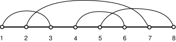
Figure 2.1. A linear Chord diagram

Without loss of generality, the smallest integer $i_{n}$ from each pairing of $X\in\mathcal{M}_{N}$ can be arranged in a strictly increasing order $1=i_{1}<i_{2}<\ldots i_{N}\leq 2N-1$. However the $j_{n}$’s are not ordered in general.

Definition 2.1.

Let ${\bf p}_{r}$ and ${\bf p}_{s}$ with $r<s$ be distinct pairings (equivalently, a pair of chords). Then,

• ${\bf p}_{r}$ and ${\bf p}_{s}$ form an alignment or a O-type configuration if $i_{r}<j_{r}<i_{s}<j_{s}$. That is, the pairs do not overlap.

• ${\bf p}_{r}$ and ${\bf p}_{s}$ form a crossing or a T-type configuration if $i_{r}<i_{s}<j_{r}<j_{s}$. That is, the pairs partially overlap.

• ${\bf p}_{r}$ and ${\bf p}_{s}$ form a nesting or a P-type configuration if $i_{r}<i_{s}<j_{s}<j_{r}$. That is the pairs completely overlap.

The meanings of O-, T-, and P-type of configurations will be clear later in Section 3 when we discuss the $N$-solitons of KPII. In Fig. 2.1, the pairing $[4,6]$ forms an alignment (O-type configuration) with $[1,3]$; a crossing with $[5,8]$; and a nesting with the pairing $[2,7]$. Furthermore, the total number of (pairwise) crossings in Fig. 2.1 is 3; they occur between the pairs $[1,3]$ and $[2,7]$; $[2,7]$ and $[5,8]$; and $[4,6]$ and $[5,8]$. Similarly, there is one nesting, $\{[2,7],[4,6]\}$, and two alignments, $\{[1,3],[4,6]\}$ and $\{[1,3],[5,8]\}$.

It should be clear that the of alignments, crossings and nestings for any $X\in\mathcal{M}_{N}$ must add up to the total number of pairwise chord configurations, i.e., $N(N-1)/2$. One of the earliest results [11, 35] in the enumeration of chord diagrams is that the number of matchings in $\mathcal{M}_{N}$ with no crossings is given by the $N^{\rm th}$ Catalan number $C_{N}=\frac{1}{N+1}\binom{2N}{N}$, which appears in many combinatorial problems (see, e.g., [33]). Similarly, the number of diagrams in $\mathcal{M}_{N}$ with no nestings is also given by $C_{N}$. The problem of counting the elements of $\mathcal{M}_{N}$ according to the number of pairwise crossings of chords was considered by Touchard [34], who gave an implicit formula for the enumerating generating function in terms of continued fractions. Subsequently, Riordan [29] derived a remarkable explicit formula for the generating function based on Touchard’s work. If $cr(X)$ denotes the number of crossings of the element $X\in\mathcal{M}_{N}$, then the generating function by the number of crossings is defined via the polynomial

$$F_{N}(q):=\sum_{X\in\mathcal{M}_{N}}\!\!q^{cr(X)}\,,\qquad 0\leq cr(X)\leq{\textstyle\frac{1}{2}}N(N-1)\,,$$

in the variable $q$ with positive integer coefficients. The Touchard-Riordan formula for $F_{N}(q)$ is

(2.1) $$F_{N}(q)=\frac{1}{(1-q)^{N}}\sum_{n=0}^{N}\!\!(-1)^{n}\left[\binom{2N}{N-n}-\binom{2N}{N-n-1}\right]q^{n(n+1)/2}\,.$$

The first few polynomials are

$$F_{1}(q)=1,\quad F_{2}(q)=q+2,\quad F_{3}(q)=q^{3}+3q^{2}+6q+5\,,$$

and it easily follows from Eq. (2.1) that the number of non-crossing diagrams is given by

$$F_{N}(0)=\binom{2N}{N}-\binom{2N}{N-1}=\frac{1}{N+1}\binom{2N}{N}\,,$$

which is the Catalan number $C_{N}$ mentioned earlier. However, the Touchard-Riordan formula is somewhat mysterious, in that it is not obvious from Eq. (2.1) that $F_{N}(q)$ is in fact a polynomial in $q$ of degree $N(N-1)/2$ as implied by its combinatorial origin, or that $F_{N}(1)=|\mathcal{M}_{N}|=(2N-1)!!$. These assertions follow only after detailed analysis of Eq. (2.1) [29] (see also [12]). A purely combinatorial proof of the Touchard-Riordan formula also appeared in Ref. [26] (see also [20]), and its relation to $q$-Hermite polynomials was investigated in ref. [18].

2.2. The $\tau$-function and line solitons of KPII

It is well known (see e.g. [31, 15]) that the solution $u(x,y,t)$ of the KPII equation is given in terms of the $\tau$-function $\tau(x,y,t)$ as

(2.2) $$u(x,y,t)=2\frac{\partial^{2}}{\partial x^{2}}\ln\tau(x,y,t)\,.$$

We consider the class of solutions whose $\tau$-functions are given by the Wronskian determinant form, i.e.,

(2.3) $$\tau(x,y,t)=\mathop{\mathrm{Wr}}\nolimits(f_{1},\dots,f_{N})=\det\begin{pmatrix}f_{1}&f_{2}&\dots&f_{N}\\ f_{1}^{\prime}&f_{2}^{\prime}&\dots&f_{N}^{\prime}\\ \vdots&\vdots&&\vdots\\ f_{1}^{(N-1)}&f_{2}^{(N-1)}&&f_{N}^{(N-1)}\end{pmatrix}\,.$$

with $f_{n}^{(j)}=\partial^{j}f_{n}/\partial x^{j}$, and where the functions $\{f_{n}\}_{n=1}^{N}$ form a set of linearly independent solutions of the linear system

$$\frac{\partial f}{\partial y}=\frac{\partial^{2}f}{\partial x^{2}}\,,\qquad\frac{\partial f}{\partial t}=\frac{\partial^{3}f}{\partial x^{3}}\,.$$

The soliton solutions of KPII can be constructed from Eq. (2.3) by choosing a finite dimensional solution for each function $f_{n}(x,y,t)$, namely,

(2.4) $$f_{n}(x,y,t)=\sum_{m=1}^{M}a_{nm}\,e^{\theta_{m}}\,,\quad n=1,2,\ldots,N\,,$$

where $\theta_{m}(x,y,t)=k_{m}x+k_{m}^{2}y+k_{m}^{3}t+\theta^{0}_{m},\,m=1,\ldots,M$, are phases with real distinct parameters $k_{1},k_{2}\ldots k_{M}$, and real constants $\theta^{0}_{1},\dots,\theta^{0}_{M}$. The constant coefficients $a_{nm}$ define the $N\times M$ coefficient matrix $A:=(a_{nm})$. The simplest example is the $1$-soliton solution with $N=1,M=2$, and $\tau=f_{1}=e^{\theta_{1}}+e^{\theta_{2}}$, for which

$$u(x,y,t)=2\frac{\partial^{2}}{\partial x^{2}}\ln\tau=\frac{1}{2}(k_{1}-k_{2})^{2}{\rm sech}^{2}\frac{1}{2}(\theta_{1}-\theta_{2})\,.$$

This $1$-soliton solution describes a plane traveling wave-form with constant amplitude $(k_{1}-k_{2})^{2}/2$. For fixed $t$, the wave-form is localized in the $(x,y)$-plane along the line $L:\theta_{1}=\theta_{2}$ whose normal has the slope $c=k_{1}+k_{2}$. The solution is characterized by two physical parameters, namely, the soliton amplitude parameter $a=|k_{1}-k_{2}|$ and the soliton direction parameter $c=k_{1}+k_{2}$.

In the general case, substitution of Eq. (2.4) into the Wronskian of Eq. (2.3), and subsequent development of the resulting determinant via Binet-Cauchy formula, yields the following explicit form of the $\tau$-function:

(2.5) $$\tau(x,y,t)=\sum_{1\leq m_{1}<\dots<m_{N}\leq M}A(m_{1},\dots,m_{N})\,\,\exp[\,\theta(m_{1},\dots,m_{N})\,]\!\!\prod_{1\leq s<r\leq N}(k_{m_{r}}-k_{m_{s}})\,,$$

where $A(m_{1},\dots,m_{N})$ is the $N\times N$ maximal minor of $A$ obtained from the columns $1\leq m_{1}<\dots<m_{N}\leq M$, and $\theta(m_{1},\dots,m_{N}):=\theta_{m_{1}}+\ldots+\theta_{m_{N}}$ is a phase combination of $N$ (out of $M$) distinct phases. Note that the transformation, $G:A\rightarrow A^{\prime}:=G\,A,\,\,G\in\mathrm{GL}(N,{\mathbb{R}})$, amounts to an overall rescaling of the minors $A(m_{1},\dots,m_{N})$, and hence, of the $\tau$-function in Eq. (2.5); i.e., $\tau\to\tau^{\prime}=\det(G)\,\tau$. Since such a rescaling leaves the solution $u(x,y,t)$ in Eq. (2.2) invariant, it is possible to reduce the coefficient matrix $A$ to reduced row-echelon form (RREF) by Gaussian elimination. Throughout the rest of this article, the coefficient matrix $A$ will be assumed to be in RREF.

The solutions $u(x,y,t)$ resulting from the $\tau$-function in Eq. (2.5) are singular for arbitrary choices of the parameters $\{k_{n}\}_{n=1}^{M}$ and the matrix $A$. To avoid such singularities, which correspond to the zero-locus of the $\tau$-function, one needs to impose certain positivity conditions.

Condition 2.2  (Positive definiteness of $\tau$).

1. The phase parameters are distinct, and are ordered as $k_{1}<k_{2}<\ldots<k_{M}$.

2. The $N\times M$ coefficient matrix $A$ satisfies $\mathop{\rm rank}\nolimits(A)=N$, and $M>N$.

3. All non-zero $N\times N$ minors of $A$ are positive.

Remark 2.3.

The matrices satisfying Condition 2.2(c) above, are called totally non-negative (TNN) matrices. The classification of the $(N_{-},N_{+})$-soliton solutions is thus given by the classification of the $N\times M$ TNN matrices $A$ in RREF. From a more geometric perspective, each TNN matrix parametrizes a unique cell in the TNN Grassmannian $Gr^{+}(N,M)$ (see e.g. [27]), and the classification of the soliton solutions corresponds to a further refinement of the Schubert decomposition of $Gr(N,M)$ into TNN Grassmann cells (see [21] for the case $M=2N$). The refinement is given by a classification of the coefficient matrix $A$ whose $N\times N$ minors $A(m_{1},\ldots,m_{N})$ represent the Plücker coordinates of $Gr(N,M)$. It should be noted that each $(N_{-},N_{+})$-soliton solution corresponding to a TNN matrix can be parametrized by a chord diagram [7, 9]. The geometric structure of this classification will be discussed in a future communication [8].

In Condition 2.2, the distinctness assumption on the set of phase parameters ensures that the set $\{e^{\theta_{m}}\}_{m=1}^{M}$ is linearly independent, while $\mathop{\rm rank}\nolimits(A)=N$ implies that the set of functions $\{f_{n}\}_{n=1}^{N}$ is linearly independent. Also when $M=N$, the sum in Eq. (2.5) reduces to a single exponential term with a phase combination that is linear in $x$. The logarithm of such a $\tau$-function is annihilated by the second derivative in Eq. (2.2), leading to the trivial solution $u(x,y,t)=0$. Thus the condition $N<M$ guarantees non-trivial solutions of KPII. Condition 2.2(c) together with the ordering $k_{1}<k_{2}<\ldots<k_{M}$ make the sum in Eq. (2.5) totally positive. As a result, $\tau(x,y,t)$ is a positive function on ${\mathbb{R}}^{3}$, and the resulting solution $u(x,y,t)$ of KPII is non-singular, bounded and positive definite. Furthermore, the asymptotic analysis of the $\tau$-function in Eq. (2.5) reveals that for any given value of $t$, there exist a set of lines given by $\{L_{ij}:\,\theta_{i}=\theta_{j},\,\,i<j\}$ in the $(x,y)$-plane, such that

(2.6) $$u(x,y,t)\sim{\textstyle\frac{1}{2}}(k_{j}-k_{i})^{2}\mathop{\rm sech}\nolimits^{2}{\textstyle\frac{1}{2}}(\theta_{j}-\theta_{i}+\delta_{ij})\,,$$

along each $L_{ij}$ either as $y\to\infty$, or as $y\to-\infty$. Equation (2.6), which has the same form as the $1$-soliton solution defines an asymptotic line soliton along $L_{ij}$ associated with the solution $u(x,y,t)$. Each line soliton which is parallel to the line $L_{ij}$ has the parameters $a_{ij}=|k_{i}-k_{j}|$ for the amplitude and $c_{ij}=k_{i}+k_{j}$ for the direction normal to the line $L_{ij}$. Hence, we denote each line soliton by the index pairing ${\bf p}=[i,j]$ labeling the line $L_{ij}$. Note from Eq. (2.4) that the indices $i,j$ labeling the phases $\theta_{i},\,\theta_{j}$ in Eq. (2.6) also label a pair of distinct columns of the coefficient matrix $A$. Due to this connection, it turns out that the pairing: ${\bf p}=[i,\,j],\,\,1\leq i<j\leq M$, of the line solitons can be determined from the structure of the coefficient matrix $A$ which is in RREF, and satisfies the following irreducibility condition.

Condition 2.4  (Irreducibility)

• Each column of $A$ contains at least one nonzero element.

• Each row of $A$ contains at least one nonzero element in addition to the pivot.

Recall that, for an $N\times M$ matrix in RREF, the leftmost non-vanishing entry in each nonzero row is called a pivot, which is normalized to unity. The index pairs $[i,j]$ of the asymptotic line solitons shown in Eq. (2.6) are then given by the following technical result, which is proved in Ref. [4].

Proposition 2.5.

Let the sub-matrices $X[ij]$ and $Y[ij]$ of $A$ be defined in terms of their column indices as

$$X[ij]:=\left[1,2,\ldots,i-1,j+1,\ldots,M\right]\qquad Y[ij]:=\left[i+1,\ldots j-1\right]\,.$$

Then, necessary and sufficient conditions for an index pair $[i,j]$ to specify an asymptotic line soliton, as in Eq. (2.6), are the following rank conditions.

1. Each line soliton as $y\to\infty$ is labeled by a unique index pair $[e_{n},j_{n}]$ with $e_{n}<j_{n}$, where $\{e_{n}\}_{n=1}^{N}$ label the pivot columns of $A$. Moreover, if $\mathop{\rm rank}\nolimits(X[e_{n}j_{n}])=:r_{n}$, then $r_{n}\leq N-1$ and

   $$\mathop{\rm rank}\nolimits(X[e_{n}\,j_{n}]|e_{n})\,\,=\,\,\mathop{\rm rank}\nolimits(X[e_{n}\,j_{n}]|j_{n})\,\,=\,\,\mathop{\rm rank}\nolimits(X[e_{n}\,j_{n}]|e_{n},j_{n})\,\,=\,\,r_{n}+1\,.$$

2. Each line soliton as $y\to-\infty$ is labeled by a unique index pair $[i_{n},g_{n}]$ with $i_{n}<g_{n}$, where $\{g_{n}\}_{n=1}^{M-N}$ label the non-pivot columns of $A$. Moreover, if $\mathop{\rm rank}\nolimits(Y[i_{n}g_{n}])=:s_{n}$, then $s_{n}\leq N-1$ and

   $$\mathop{\rm rank}\nolimits(Y[i_{n}\,g_{n}]|i_{n})\,\,=\,\,\mathop{\rm rank}\nolimits(Y[i_{n}\,g_{n}]|g_{n})\,\,=\,\,\mathop{\rm rank}\nolimits(Y[i_{n}\,g_{n}]|i_{n},g_{n})\,\,=\,\,s_{n}+1\,.$$

Here $(Z|m,n)$ denotes the sub-matrix $Z$ of $A$ augmented by the columns $m$ and $n$ of $A$.

It should be clear from the above result that the $(N_{-},N_{+})$-soliton solution of KPII generated from the $\tau$-function in Eq. (2.5) has exactly $N_{+}=N$ asymptotic line-solitons as $y\to\infty$ and $N_{-}=M-N$ asymptotic line-solitons as $y\to-\infty$. From the $\tau$-function data consisting of $M$ distinct phase parameters $k_{1},\ldots,k_{M}$ and a matrix $A$ satisfying Condition 2.3, Proposition 2.5 provides an explicit way to identify all the asymptotic line solitons of the corresponding solution of the KPII equation. We illustrate this method with an example.

Example 2.6.

Consider the solution $u(x,y,t)$ generated by the $\tau$-function of Eq. (2.3) in the case $N=2$ and $M=4$, with 4 real parameters $k_{1}<k_{2}<k_{3}<k_{4}$, and

$$f_{1}=e^{\theta_{1}}-e^{\theta_{4}},\quad f_{2}=e^{\theta_{2}}+e^{\theta_{3}},\qquad\qquad A=\begin{pmatrix}1&0&0&\!-1\\ 0&1&1&0\end{pmatrix}\,.$$

The pivot columns of $A$ are labeled by the indices $\{e_{1},e_{2}\}=\{1,2\}$, and the non-pivot columns by the indices $\{g_{1},g_{2}\}=\{3,4\}$. According to Proposition 2.5, the number of asymptotic line solitons is $N_{+}=N_{-}=2$. They are identified by the index pairs $[1,j_{1}],\,[2,j_{2}]$ as $y\to\infty$, for some $j_{1}>1$ and $j_{2}>2$; and by the index pairs $[i_{1},3]\,,[i_{2},4]$ as $y\to-\infty$, for some $i_{1}<3$ and $i_{2}<4$. We first determine the asymptotic line-solitons as $y\to\infty$ using the rank conditions prescribed in Proposition 2.5(i). For the first pivot column $e_{1}=1$; starting from $j=2$ and then repeatedly incrementing the value of $j$ by unity, we check the rank of each sub-matrix $X[1j]$. Proceeding in this way, we find that the rank conditions are satisfied only when $j=4$: $X[14]=\emptyset$. So, $\mathop{\rm rank}\nolimits(X[14])=0<N-1$. Moreover, $\mathop{\rm rank}\nolimits(X[14]|1)=\mathop{\rm rank}\nolimits(X[14]|4)=\mathop{\rm rank}\nolimits(X[14]|1,4)=1$ since columns 1 and 4 are parallel. Thus, the first asymptotic line soliton as $y\to\infty$ is identified by the index pair $[1,4]$. For $e_{2}=2$, proceeding in a similar manner we find that $j=3$ does satisfy the rank conditions since $X[23]=\bigl{(}\begin{smallmatrix}1&-1\\ 0&0\end{smallmatrix}\bigr{)}$ is of rank $1=N-1$, and $\mathop{\rm rank}\nolimits(X[23]|2)=\mathop{\rm rank}\nolimits(X[23]|3)=\mathop{\rm rank}\nolimits(X[23]|2,3)=2$. Therefore, the asymptotic line solitons as $y\to\infty$ are identified with the index pairs $[1,4]$ and $[2,3]$.

We next consider the asymptotics for $y\to-\infty$. Starting with the non-pivot column $g_{1}=3$, we apply the rank conditions in Proposition 2.5(ii) to the column $i=2$. Then, we have $Y[23]=\emptyset$, and $\mathop{\rm rank}\nolimits(Y[23]|2)=\mathop{\rm rank}\nolimits(Y[23]|3)=\mathop{\rm rank}\nolimits(Y[23]|2,3)=1$. Hence, the pair $[2,3]$ identifies an asymptotic line-soliton as $y\to-\infty$. For $g_{2}=4$, we consider $i=1,2,3$ and find that the rank conditions are satisfied only for $i=1$. In this case, $Y[14]=\bigl{(}\begin{smallmatrix}0&0\\ 1&1\end{smallmatrix}\bigr{)}$, so $\mathop{\rm rank}\nolimits(Y[14])=1=N-1$ and $\mathop{\rm rank}\nolimits(Y[14]|1)=\mathop{\rm rank}\nolimits(Y[14]|4)=\mathop{\rm rank}\nolimits(Y[14]|1,4)=2$. Thus, the index pair $[1,4]$ identifies the other asymptotic line-soliton as $y\to-\infty$. In summary, both pairs of asymptotic line solitons as $y\to\pm\infty$ are labeled by the index pairs $[1,4]$ and $[2,3]$. This is an example of a P-type $2$-soliton solution (see Section 3), and is shown in Fig. 3.1.

It should be emphasized that in general $N_{-}\neq N_{+}$, and that even in the case $N_{-}=N_{+}$, the line solitons as $y\to\infty$ are in general distinct from the line solitons as $y\to-\infty$ in both amplitude and direction. In this article, we restrict our discussions primarily to the $N$-soliton subclass of the line-soliton solutions of KPII.

Definition 2.7.

Let $S_{+}:=\{[e_{n},j_{n}]\}_{n=1}^{N}$ and $S_{-}:=\{[i_{n},g_{n}]\}_{n=1}^{M-N}$ denote the index sets identifying the line solitons as $y\to\infty$ and as $y\to-\infty$, respectively, according to Proposition 2.5. Then two $(N_{-},N_{+})$-soliton solutions of KPII are said to be in the same equivalence class if their asymptotic line-solitons are labeled by identical sets $S_{\pm}$ of index pairs, where $|S_{+}|:=N_{+}=N$ and $|S_{-}|:=N_{-}=M-N$.

The set $S_{+}\cup S_{-}$ of unique index pairings in Definition 2.7 has a combinatorial interpretation. Let $[M]:=\{1,2,\ldots,M\}$ be the integer set with the pivot and non-pivot indices $\{e_{1},\ldots,e_{N}\}\cup\{g_{1},\ldots,g_{M-N}\}$ forming a disjoint partition of $[M]$. Define the pairing map $\pi:[M]\to[M]$ according to Proposition 2.5(i) & (ii) as

(2.7) $$\pi(e_{n})=j_{n}\,,\,\,n=1,2,\ldots,N\,,\qquad\pi(g_{n})=i_{n}\,,\,\,n=1,2,\ldots,M-N\,.$$

Then $\pi:[M]\to[M]$ is a bijection, i.e., $\pi\in\mathcal{S}_{M}$, the permutation group of $[M]$ [7]. In addition, Proposition 2.5 implies the following.

Proposition 2.8.

The pairing map $\pi$ defined by Eq. (2.7) is a derangement of $[M]$ with $N$ excedances, which are given by the pivot indices $\{e_{1},\ldots,e_{N}\}$ of the coefficient matrix $A$ in RREF.

Recall that a permutation $\pi$ with no fixed point is called a derangement, and an element $l\in[M]$ is called an excedance of $\pi$ if $\pi(l)>l$.

Each equivalence class of $(N_{-},N_{+})$-soliton solutions of KPII is uniquely determined by a derangement $\pi$, as in Proposition 2.8. These derangements also give a unique parametrization of a TNN Grassmann cell (see Remark 2.3) whose associated TNN matrix $A$ satisfies the irreducibility Condition 2.3. Recall that in Example 2.6, both sets of line solitons as $y\to\pm\infty$ are given by $[1,4],\,[2,3]$, where 1,2 are the pivot indices and 3,4 are the non-pivot indices of the associated coefficient matrix $A$. In this case, the pairing map is a derangement of the set $[4]$, and is given by

$$\pi=\begin{pmatrix}1&2&3&4\\ 4&3&2&1\end{pmatrix}\in\mathcal{S}_{4}\,,$$

in the bi-word notation of permutations in $\mathcal{S}_{4}$. Note that the excedance set of $\pi$ is $\{1,2\}$. In addition, $\pi$ is also an involution of $\mathcal{S}_{4}$, i.e., $\pi^{-1}=\pi$. Since the set of all involutions of $\mathcal{S}_{2N}$ is isomorphic to the set of perfect matchings $\mathcal{M}_{N}$ introduced in Section 2.1, the involutions can be also represented by the chord diagrams representing the elements of $\mathcal{M}_{N}$. In particular, the chord diagram for the involution $\pi\in\mathcal{S}_{4}$ given above depicts a nesting of the chords ${\bf p}_{1}=[1,4]$ and ${\bf p}_{2}=[2,3]$ as shown below in Fig. 3.1. We remark that it is possible to represent derangements that are not involutions by linear chord diagrams, with directed chords both above and below the line. These diagrams have been used to study the more general $(N_{-},N_{+})$-soliton solutions of KPII in Ref. [7]. But here we focus our attention to the $N$-soliton solutions, which will be our next topic of discussion.

3. $N$-soliton solutions

When $M=2N$, it follows from Proposition 2.5 that $N_{-}=N_{+}=N$. If in addition, we consider $S_{-}=S_{+}$ in Definition 2.7, then we recover the interesting subclass of the $(N,N)$-soliton solutions mentioned in Section 1, called $N$-soliton solutions, which are characterized by identical sets of asymptotic line-solitons as $|y|\to\infty$. Then the main features of the $N$-soliton solutions follow primarily from our discussion in Section 2, in particular from Propositions 2.5 and  2.8. These are listed below.

Property 3.1  $N$-soliton solutions have the following properties.

1. The $\tau$-function of an $N$-soliton solution is expressed in terms of $2N$ distinct phase parameters and an $N\times 2N$ coefficient matrix $A$ which satisfies Conditions 2.2 and 2.3. In addition, the $N\times N$ minors of $A$ satisfy the duality conditions [7, 21]:

   $$A(m_{1},\ldots,m_{N})=0\qquad\Longleftrightarrow\qquad A(l_{1},\ldots,l_{N})=0\,,$$

   where the indices $\{m_{1},\ldots,m_{N}\}$ and $\{l_{1},\ldots,l_{N}\}$ form a disjoint partition of integers $\{1,2,\ldots,2N\}$. That is, the phase combination $\theta(m_{1},\ldots,m_{N})$ is present in the $\tau$-function of Eq. (2.5) if and only if $\theta(l_{1},\ldots,l_{N})$ is.

2. Each $N$-soliton solution has exactly $N$ asymptotic line solitons as $y\to\pm\infty$ identified by the same index pairs $[e_{n},g_{n}]$ with $e_{n}<g_{n},\,n=1,\ldots,N$. The sets $\{e_{1},\ldots,e_{N}\}$ and $\{g_{1},\ldots,g_{N}\}$ label respectively the pivot and non-pivot columns of the coefficient matrix $A$. Hence, they form a disjoint partition of the integer set $[2N]$.

3. The amplitude and direction parameters of the $n^{\mathrm{th}}$ asymptotic line soliton $[e_{n},g_{n}]$ are the same as $y\to\pm\infty$, and are given in terms of the phase parameters as

   $$a_{n}=k_{g_{n}}-k_{e_{n}}\,,\qquad\qquad c_{n}=k_{g_{n}}+k_{e_{n}}\,.$$

4. The pairing map associated to an $N$-soliton solution, namely $\pi(e_{n})=g_{n},\,\pi(g_{n})=e_{n},\,\,n=1,2,\ldots,N$, corresponds to a partition of the integer set $[2N]$ into $N$ distinct pairs of integers $(e_{n},g_{n})$, as in Section 2.1. Each such map is an involution in $\mathcal{S}_{2N}$ with no fixed points, a member of

   $$\mathcal{I}_{2N}=\{\pi\in\mathcal{S}_{2N}:\,\pi^{-1}=\pi\,\mbox{and}\,\pi(i)\neq i,\,\forall\,i\in[2N]\}\,.$$

   Such permutations can be expressed as products of $N$ disjoint $2$-cycles, and their chord diagrams are identical to those of the perfect matchings $\mathcal{M}_{N}$ (see Fig. 2.1). The total number of such involutions is given by $|I_{2N}|=|\mathcal{M}_{N}|=(2N-1)!!$. Hence, there are $(2N-1)!!$ distinct equivalence classes of $N$-soliton solutions.

3.1. Equivalence classes of 2-soliton solutions

When $N=2$, there are three types of 2-soliton solutions referred to as the O-, T- and P-types (following the terminology introduced in Ref. [21]). They are identified by the canonical coefficient matrices associated with $\tau$-functions, namely

(3.1) $$A_{\mathrm{O}}=\begin{pmatrix}1&1&0&0\\ 0&0&1&1\end{pmatrix},\qquad A_{\mathrm{T}}=\begin{pmatrix}1&0&-1&-1\\ 0&1&x_{1}&x_{2}\end{pmatrix},\qquad A_{\mathrm{P}}=\begin{pmatrix}1&0&0&-1\\ 0&1&1&0\end{pmatrix},$$

with $x_{1}>x_{2}>0$ in $A_{\mathrm{T}}$. By applying the rank conditions of Proposition 2.5 to the above coefficient matrices, it is easily verified that the O-type 2-solitons have asymptotic line-solitons [1,2] and [3,4]; the T-type resonant 2-solitons have asymptotic line-solitons [1,3] and [2,4]; and the P-type 2-solitons have asymptotic line-solitons [1,4] and [2,3]. These are shown in Fig. 3.1. Notice that each of the O- and P-type solitons interact via an X-junction. After interaction, each line soliton undergoes a position shift in the $xy$-plane. However, it can be shown that the position shifts for the O-type solitons are opposite in sign to that of the P-type solitons [7]. On the other hand, the T-type solitons interact via four Y-junctions, connecting the four asymptotic line-solitons to four intermediate segments. Each of these intermediate segments is also a line soliton.

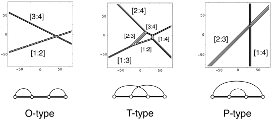
Figure 3.1. Three different two-soliton solutions of KPII with the same phase parameters $(k_{1},\dots,k_{4})=(-2,-\frac{1}{2},0,1)$, illustrating the three $2$-soliton equivalence classes: O-type, T-type and  P-type 2-soliton solutions.

For example, in the T-type solitons in Fig. 3.1 the asymptotic line soliton $[1,3]$ (as $y\to-\infty$) forms the intermediate line-solitons $[1,2]$ and $[2,3]$ at the bottom left Y-junction. The line-soliton $[2,3]$ connects with the asymptotic line-soliton $[2,4]$ (as $y\to\infty$) and the line-soliton $[1,2]$ connects with the asymptotic line soliton $[2,4]$ (as $y\to-\infty$). Similarly, the asymptotic line soliton $[1,3]$ (as $y\to\infty$) forms the intermediate line-solitons $[1,4]$ and $[3,4]$ at the top right Y-junction. The line-soliton $[3,4]$ connects with the asymptotic line-soliton $[2,4]$ (as $y\to\infty$) and the line-soliton $[1,4]$ connects with the asymptotic line soliton $[2,4]$ (as $y\to-\infty$). Fig. 3.1 also shows the chord diagrams for the corresponding pairing maps, which are involutions of the permutation group ${\mathcal{S}}_{4}$. They correspond to the disjoint partitions of $[4]$ into 2 pairs. In cycle notation, these involutions are given by $\pi_{\mathrm{O}}=(12)(34),\,\pi_{\mathrm{T}}=(13)(24)$, and $\pi_{\mathrm{P}}=(14)(23)$, for the O-, T- and P-type $2$-soliton equivalence classes. According to the Definition 2.1, the chord diagram for $\pi_{\mathrm{O}}$ forms an alignment; whereas the diagram for $\pi_{\mathrm{T}}$ has a crossing between the chords corresponding to the line solitons $[1,3]$ and $[2,4]$; and the diagram for $\pi_{\mathrm{P}}$ is a nesting.

An important distinction among the three types of 2-soliton solutions is that they belong to different regions of the soliton parameter space. Suppose $(a_{1},c_{1})$ and $(a_{2},c_{2})$ are the soliton parameters of the asymptotic line-solitons of each type, with the same set of distinct phase parameters. Since the phase parameters are ordered: $k_{1}<\dots<k_{4}$, the soliton parameters satisfy the following relations, which can be easily verified using Eqs. ((iii)).

1. For O-type 2-soliton solutions, $c_{2}>c_{1}$ and $c_{2}-c_{1}>a_{1}+a_{2}$.

2. For T-type 2-soliton solutions, $c_{2}>c_{1}$, and $|a_{1}-a_{2}|<c_{2}-c_{1}<a_{1}+a_{2}$.

3. For P-type 2-soliton solutions, $a_{2}>a_{1}$ and $|c_{2}-c_{1}|<a_{2}-a_{1}$.

4. $(c_{2}-c_{1})_{\mathrm{O}}>(c_{2}-c_{1})_{\mathrm{T}}>|c_{2}-c_{1}|_{\mathrm{P}}$ ,  $(a_{1}+a_{2})_{\mathrm{O}}<(a_{1}+a_{2})_{\mathrm{T}}=(a_{1}+a_{2})_{\mathrm{P}}$ , and
   $|a_{2}-a_{1}|_{\mathrm{O}}=|a_{2}-a_{1}|_{\mathrm{T}}<(a_{2}-a_{1})_{\mathrm{P}}$ .

Note that for O- and T-type solutions the soliton directions are ordered, while for P-type solutions the amplitudes are ordered. Any choice of the soliton parameters $a_{1},c_{1};a_{2},c_{2}$ with $a_{1},a_{2}>0$ would lead to one of the three types of 2-soliton solutions, provided that $\{c_{1}\pm a_{1},\,c_{2}\pm a_{2}\}$ are distinct real numbers. Thus, the three types of 2-soliton solutions partition the soliton parameter space into disjoint sectors, bounded by the hyperplanes $|c_{2}-c_{1}|=a_{1}+a_{2}$ and $|c_{2}-c_{1}|=|a_{1}-a_{2}|$. At each boundary between two sectors, two of the phase parameters coincide. In such a situation, it can be shown (by taking suitable limits) that the 2-soliton solution degenerates into a Y-junction [6, 21].

It should be clear from the above that the O-, T- and P-type $2$-soliton solutions exhibit distinct types of interaction patterns, and belong to different regions of the soliton parameter space. For $N>2$, in addition to the non-resonant (O- and P-type) and fully resonant (T-type) solutions, a large family of partially resonant solutions exists. For example, when $N=3$, Property 3(iv) implies that there are 15 distinct equivalent classes of $3$-soliton solutions (see Fig.3.2). Unlike the $N=2$ case above, it turns out to be a complicated task to classify the $N$-soliton solutions according to their coefficient matrices $A$, when $N>2$. This task was recently carried out by the authors, and will be reported in a future publication [8]. Here we consider a more direct classification scheme for the $N$-soliton equivalence classes, by characterizing the pairwise interactions between the $N$ line solitons of O-, T- and P-type, much as in the $2$-soliton case. In other words, we represent the $N$-soliton solutions by the corresponding involutions in $\mathcal{I}_{2N}\subset\mathcal{S}_{2N}$ (equivalently, the matchings in ${\mathcal{M}}_{N}$), and enumerate the solutions according to the number of alignments, crossings and nestings of the associated chord diagram. We describe this classification scheme below.

3.2. Combinatorics of $N$-soliton solutions

Throughout this subsection, we associate an $N$-soliton equivalence class defined by the set $S=\{[e_{n},g_{n}]\}_{n=1}^{N}$ of asymptotic line solitons (see Definition 2.7) with the partition $X=\{{\bf p}_{1},{\bf p}_{2},\ldots,{\bf p}_{N}\}\in\mathcal{M}_{N}$, where ${\bf p}_{n}:=[e_{n},g_{n}]$. Recall from Property 3(ii) that the integer set $[2N]$ is a disjoint union of the index sets $E:=\{e_{1},\ldots,e_{N}\}$ and $G:=\{g_{1},\ldots,g_{N}\}$, with the following orderings among the indices:

(i)  $1=e_{1}<e_{2}<\ldots<e_{N}<2N$,

(ii) $e_{n}<g_{n}$ for all $n=1,2,\ldots,N$.
An immediate consequence of the above orderings is that

(3.2) $$n\leq e_{n}\leq 2n-1\,,\qquad n=1,\ldots,N\,,$$

since there are at least $n-1$ indices to the left of $e_{n}$, namely $e_{1},e_{2},\ldots,e_{n-1}$; and at least $2N-2n+1$ indices to the right of $e_{n}$, namely $g_{n},e_{r},g_{r},\,\,r>n$. The $N$-soliton classification scheme is obtained by considering various statistics over the possible chord configurations for the chord diagrams of $\mathcal{M}_{N}$. For this purpose, using Definition 2.1 we introduce the following sets, which record the total number of alignments, crossings and nestings for a given chord in any chord diagram of $\mathcal{M}_{N}$.

Definition 3.2.

Let ${\bf p}_{n}=[e_{n},g_{n}]$ be a given chord of a partition $X\in\mathcal{M}_{N}$, and let $B_{n}:=\{{\bf p}_{r}=[e_{r},g_{r}]\,:\,r<n\}$ be the subset of chords originating from the left of ${\bf p}_{n}$ in the linear chord diagram of $X$.

1. The set $O_{n}$ of alignments with the chord ${\bf p}_{n}$ forming O-type configurations, and the alignment number $al(X)$, are defined by

   $$O_{n}:=\{{\bf p}_{r}=[e_{r},g_{r}]\in B_{n}\,:\,g_{r}<e_{n}\}\,,\qquad al(X):=\sum_{n=1}^{N}|O_{n}|\,.$$

2. The set $T_{n}$ of crossings with the chord ${\bf p}_{n}$ forming T-type configurations, and the crossing number $cr(X)$, are defined by

   $$T_{n}:=\{{\bf p}_{r}=[e_{r},g_{r}]\in B_{n}\,:\,e_{n}<g_{r}<g_{n}\}\,,\qquad cr(X):=\sum_{n=1}^{N}|T_{n}|\,.$$

3. The set $P_{n}$ of nestings with the chord ${\bf p}_{n}$ forming P-type configurations, and the nesting number $ne(X)$, are defined by

   $$P_{n}:=\{{\bf p}_{r}=[e_{r},g_{r}]\in B_{n}\,:\,g_{r}>g_{n}\}\,,\qquad ne(X):=\sum_{n=1}^{N}|P_{n}|\,.$$

It follows from the above definitions that $B_{n}$ is the disjoint union of the sets $O_{n},\,T_{n}$ and $P_{n}$, so that $|O_{n}|+|T_{n}|+|P_{n}|=n-1$, and $al(X)+cr(X)+ne(X)=N(N-1)/2$, which is a count of all possible pairwise chord configurations in the partition $X$. Note that for $O_{n}$, the indices $g_{r}$ lie in the intervals $(e_{r},e_{r+1}),\,\,1\leq r<n$. Hence, $|O_{n}|=e_{n}-n$. So the number of crossings and nestings with the chord ${\bf p}_{n}$ sum to $|T_{n}|+|P_{n}|=(n-1)-(e_{n}-n)=2n-e_{n}-1$, which depends only on the pivot index $e_{n}\in E$. This observation leads to the following.

Lemma 3.3.

If $\mathcal{M}(E)\subseteq\mathcal{M}_{N}$ denotes the set of all partitions which have the same (pivot) index set $E$, then the number of partitions of $\mathcal{M}(E)$ having $r$ crossings and $s$ nestings is the coefficient of $p^{s}q^{r}$ in

$$m_{E}(p,q)=\prod_{n=1}^{N}\,[2n-e_{n}]_{p,q}\,,\qquad[n]_{p,q}:=\frac{p^{n}-q^{n}}{p-q}=\sum_{i+j=n-1}p^{i}q^{j}\,.$$

The degree of both $p$ and $q$ in $m_{E}(p,q)$ is $N^{2}-(e_{1}+e_{2}+\ldots+e_{N})$.

Proof 3.4.

The distribution of crossings and nestings is the sum of $p^{ne(X)}q^{cr(X)}$ over all partitions $X\in\mathcal{M}(E)$. Using Definition 3.2 for $cr(X)$ and $ne(X)$, this distribution can be expressed as

$$\sum_{X\in\mathcal{M}(E)}p^{(|P(1)|+\ldots+|P(N)|)}q^{(|T(1)|+\ldots+|T(N)|)}=\prod_{n=1}^{N}\sum_{l=0}^{2n-e_{n}-1}p^{l}q^{2n-e_{n}-1-l}\,,$$

after interchanging the sum and product, and using the fact that $|T_{n}|+|P_{n}|=2n-e_{n}-1$ for $n=1,2,\ldots,N$. Since the second sum is precisely $[2n-e_{n}]_{p,q}$, the formula for $m_{E}(p,q)$ follows.

It is easy to verify from the product formula that $m_{E}(p,q)$ is symmetric in $p$ and $q$. Consequently, the number of diagrams with $r$ crossings and $s$ nestings is the same as the the number of diagrams with $s$ crossings and $r$ nestings [20]. Note also that the enumerating polynomial for the crossings alone is given by $m_{E}(1,q)$; while $m_{E}(p,1)$ enumerates only the nestings for the chord diagrams of $\mathcal{M}(E)$. In order to extend the results of Lemma 3.3, to the entire set $\mathcal{M}_{N}$, one needs to sum $m_{E}(p,q)$ over all possible choices of the integer set $E$, with $e_{n}\in E$ satisfying Eq. (3.2). Using Lemma 3.3, the expression for the required generating polynomial is given by

(3.3) $$F_{N}(p,q):=\sum_{X\in\mathcal{M}_{N}}p^{ne(X)}q^{cr(X)}=\sum_{\{E\}}m_{E}(p,q)=\sum_{\genfrac{}{}{0.0pt}{1}{1=e_{1}<e_{2}<\ldots<e_{N},}{k\leq e_{k}\leq 2k-1}}\,\prod_{n=1}^{N}[2n-e_{n}]_{p,q}\,.$$

Since we have from Eq. (3.2) that $e_{n}\geq n,\,n=1,2,\ldots,N$, it follows from Lemma 3.3 that the degree of $p$ and $q$ in $F_{N}(p,q)$ is given by

$$ne(X)_{\mathrm{m}ax}=cr(X)_{\mathrm{m}ax}=N^{2}-(1+2+\ldots+N)=\frac{N(N-1)}{2}\,.$$

Furthermore, like $m_{E}(p,q)$, $F_{N}(p,q)$ is symmetric in $p$ and $q$, i.e.,

$$F_{N}(p,q)=\sum_{r,s=0}^{N(N-1)/2}c_{rs}q^{r}p^{s}\,,\qquad c_{rs}=c_{sr}\,.$$

Some interesting consequences of Eq. (3.3) for special cases of $F_{N}(p,q)$ are collected below.

Corollary 3.5.

The function $F_{N}(p,q)$ has the following properties:

• $F_{N}(1,1)=|\mathcal{M}_{N}|=(2N-1)!!$.

• When $p=1,q=0$, the total number of non-crossing (i.e., only alignments and nestings) chord diagrams of $\mathcal{M}_{N}$ equals the $N^{\mathrm{t}h}$ Catalan number [11]. That is, $F(1,0)=C_{N}$ which also counts the total possible choices for the ordered integer set $E$ [7]. Similarly, $F_{N}(0,1)=C_{N}$ gives the total number of non-nesting (i.e., only alignments and crossings) chord diagrams of $\mathcal{M}_{N}$.

• $F_{N}(1,q)=:F_{N}(q)$ gives the generating polynomial for the number of crossings introduced in Section 2.1, which is given explicitly by the Touchard-Riordan formula Eq. (2.1).

The polynomials $F_{N}(p,q)$ can be determined from a generating function $F(p,q,x)$ which is a formal power series, and has the following representation.

Proposition 3.6.

The generating function for $F_{N}(p,q)$ is the Stieltjes-type continued fraction, namely

$$F(p,q,x):=\sum_{N=0}^{\infty}F_{N}(p,q)x^{N}=\cfrac{1}{1-\cfrac{x\,[1]_{p,q}}{1-\cfrac{x\,[2]_{p,q}}{1-\cfrac{x\,[3]_{p,q}}{1-\cdots}}}}\,,\qquad F_{0}(p,q):=1\,.$$

Proof 3.7.

First consider the set $E:=\{1=e_{1}<\cdots<e_{N}:e_{k}\leq 2k-1\}$. Note that $E$ can be decomposed into distinct subsets when $e_{n}=2n-1$. One has

$$E=\bigcup_{n=0}^{N-1}\left(E_{n}\cup\hat{E}_{n}\right)\,,$$

where $E_{n}:=\{1=e_{1}<\cdots<e_{n}:\,e_{k}\leq 2k-1\}$ for $n\neq 0$ can be viewed as the $n$-truncates of the original set $E$, $E_{0}=\varnothing$, and

$$\hat{E}_{n}:=\{2n+1=e_{n+1}<\cdots<e_{N}:\,2n+k\leq e_{n+k}<2(n+k)-1\}\,.$$

The set $\hat{E}_{n}$ can be re-expressed as

$$E^{\prime}_{N-n}=\{1=e^{\prime}_{1}<\cdots<e^{\prime}_{N-n}:\,k\leq e^{\prime}_{k}<2k-1\}\,,$$

by shifting and relabeling the indices as $e_{n+k}:=e^{\prime}_{k}+2n$. Note however that $E^{\prime}_{N-n}$ (with all $e^{\prime}_{k}<2k-1$) is not the same as $E_{N-n}$ (with all $e_{k}\leq 2k-1$).

From Eq. (3.3),

(3.4) $$F_{N}(p,q)=\sum_{\{E\}}\,\prod_{k=1}^{N}\,[2k-e_{k}]_{p,q}=\sum_{n=0}^{N-1}F_{n}(p,q)C_{N-n}(p,q)\,,$$

where $C_{n}(p,q)=\displaystyle\sum_{\{E^{\prime}_{n}\}}\displaystyle\,\prod_{k=1}^{n}\,[2k-e^{\prime}_{k}]_{p,q}$. Introduce the power series

$$F(p,q,x)=\sum_{N=0}^{\infty}F_{N}(p,q)x^{N}\,,\quad F_{0}(p,q):=1\,,$$

$$C(p,q,x)=\sum_{N=1}^{\infty}C_{N}(p,q)x^{N}\,.$$

Using Eq. (3.4) in the power series, one finds that $F(p,q,x)-1$ equals the product $F(p,q,x)C(p,q,x)$, which implies

(3.5) $$F(p,q,x)=\frac{1}{1-C(p,q,x)}\,.$$

Next, define the associated polynomials

$$F_{n}(p,q;l):=\sum_{\{E_{n}\}}\prod_{k=1}^{n}[2k-e_{k}+l]_{p,q}\,,\quad C_{n}(p,q;l):=\sum_{\{E^{\prime}_{n}\}}\prod_{k=1}^{n}[2k-e^{\prime}_{k}+l]_{p,q}\,,$$

so that $F_{n}(p,q;0)=F_{n}(p,q)$ and $C_{n}(p,q;0)=C_{n}(p,q)$. The corresponding power series $F(p,q;l,x)$ and $C(p,q;l,x)$ are defined similarly to $F(p,q,x)$ and $C(p,q,x)$ above, and they also satisfy Eq.(3.5). Furthermore, for $n>1$ the associated polynomials satisfy the relation

(3.6) $$C_{n}(p,q;l)=\sum_{\{E^{\prime}_{n}\}}\prod_{k=1}^{n}[2k-e^{\prime}_{k}+l]_{p,q}=[l+1]_{p,q}\sum_{\{E^{\prime}_{n}\}}\prod_{k=2}^{n}[2k-e^{\prime}_{k}+l]_{p,q}$$

(3.7) $$=[l+1]_{p,q}\sum_{\{E_{n-1}\}}\prod_{j=1}^{n-1}[2j-e_{j}+(l+1)]_{p,q}=[l+1]_{p,q}F_{n-1}(p,q;l+1)\,,$$

after an appropriate index shift, $k=j+1$, and relabelings $e^{\prime}_{j+1}=e_{j}+1$ so that $j\leq e_{j}\leq 2j-1$ for $j=1,\ldots n-1$. As a result, the set $E^{\prime}_{n}$ changed to the set $E_{n-1}$. The formal power series constructed from the first and last expressions in Eq.(3.7) satisfies $C(p,q;l,x)=x[l+1]_{p,q}F(p,q;l+1,x)$. From the analogue of Eq. (3.5) for the associated functions $F(p,q;l,x)$ and $C(p,q;l,x)$, one therefore obtains

$$F(p,q;l,x)=\frac{1}{1-[l+1]_{p,q}xF(p,q;l+1,x)}\,.$$

This yields the continued fraction representation for $F(p,q,x)=F(p,q;0,x)$.

We can graphically illustrate the results of Proposition 3.6 for $N=2$ and 3 in terms of the corresponding chord diagrams. For $N=2$, $F_{2}(p,q)=1+p+q$, which implies that there is one each of the O-, T-, and P-type diagrams. These were displayed in Fig. 3.1. For $N=3$, there are 15 chord diagrams, which are displayed in Fig.3.2. They are characterized by

$$F_{3}(p,q)=(1+2p+p^{2}+p^{3})+(2+2p+2p^{2})q+(1+2p)q^{2}+q^{3}\,.$$

Note that the total number of pairwise chord configurations for each case for $N=3$ is 3(3-1)/2 = 3. We use the ordering $({\bf p}_{1}{\bf p}_{2},\,{\bf p}_{2}{\bf p}_{3},\,{\bf p}_{3}{\bf p}_{1})$ for the chord-pairs, and indicate the interaction type for each pair below:

1. Non-resonant cases:   1 (PPP)-type, 1 (PPO)-type, 2 (POO)-type, 1 (OOO)-type. These are on the first row in Fig.3.2, from left to right.

2. One-resonant cases:    2 (TPP)-type, 2 (TPO)-type, and 2 (TOO)-type. These are on the second row.

3. Two-resonant cases:   2 (TTP)-type and 1 (TTO)-type. These are on the the third row.

4. Three- (i.e., fully-) resonant case: 1 (TTT)-type.

Figure 3.2. The closed chord diagrams for $3$-soliton solutions. The dots indicate the pivots $(e_{1},e_{2},e_{3})$, and the ordered letters below each diagram indicate the type of interactions in $({\bf p}_{1}{\bf p}_{2},{\bf p}_{2}{\bf p}_{3},{\bf p}_{3}{\bf p}_{1})$ with the soliton pairing ${\bf p}_{n}=[e_{n},g_{n}]$. The number of the diagrams having the same number of crossings comes from the generating function $F_{3}(q)=q^{3}+3q^{2}+6q+5$. E.g., 5, the Catalan number $C_{3}=F_{3}(0)$, counts the diagrams in the first row.

3.3. Generating function and $q$-orthogonal polynomials

In the special case when $p=1$, the formula for $F(q,x):=F(1,q,x)$ in Proposition 3.6 reduces to similar continued fraction expression for $F(q,x):=F(1,q,x)$, namely

(3.8) $$F(q,x)=\sum_{N=0}^{\infty}F_{N}(q)x^{N}=\cfrac{1}{1-\cfrac{x\,[1]_{q}}{1-\cfrac{x\,[2]_{q}}{1-\cfrac{x\,[3]_{q}}{1-\cdots}}}}\,,\qquad F_{0}(q):=1\,,$$

with $[n]_{q}:=1+q+\ldots+q^{n-1}$. From Corollary 3.5(iii), it follows that $F(q,x)$ is the generating function for the polynomials $F_{N}(q)$ that enumerate the crossings of the chords of $\mathcal{M}_{N}$, whose explicit formula is given by Eq. (2.1). Here we show that the continued fraction for $F(q,x)$ is related to the moment generating function for the continuous $q$-Hermite polynomials. It follows that the Touchard-Riordan polynomials $F_{N}(q)$ are simply the even moments of the weight function with respect to which the $q$-Hermite polynomials are orthogonal. The latter result was also found in Ref. [18].

We first collect some facts (see e.g. [10, 22]) from the spectral theory of bounded, real, semi-infinite Jacobi matrices on the Hilbert space

$$l_{2}(\mathbb{C}):=\{u=(u_{0},u_{1},u_{2},\ldots)\,:\,u_{i}\in\mathbb{C}\,,\quad\sum_{k=0}^{\infty}|u_{k}|^{2}<\infty\}\,.$$

Define the following tri-diagonal matrices

$$L:=\begin{pmatrix}0&1&0&\cdots\\ a_{1}&0&1&\cdots\\ 0&a_{2}&0&\ddots\\ \vdots&\ddots&\ddots&\ddots\end{pmatrix}\quad L_{n}:=\begin{pmatrix}0&1&0&\cdots&0\\ a_{1}&0&1&\cdots&0\\ \vdots&\ddots&\ddots&\ddots&\vdots\\ 0&\cdots&a_{n-2}&0&1\\ 0&\cdots&0&a_{n-1}&0\end{pmatrix}\quad\widehat{L}_{n-1}:=\begin{pmatrix}0&1&0&\cdots&0\\ a_{2}&0&1&\cdots&0\\ \vdots&\ddots&\ddots&\ddots&\vdots\\ 0&\cdots&a_{n-2}&0&1\\ 0&\cdots&0&a_{n-1}&0\end{pmatrix}\,,$$

with $a_{i}>0,\,i=1,2,\ldots$. Next, consider the linear system of equations

$$(\lambda I-L)\varphi=e_{0}\,,\quad{\rm for}\quad\varphi=(\varphi_{0},\varphi_{1},\varphi_{2},\ldots)^{T}\,,$$

where $I:=\mathop{\rm diag}\nolimits(1,1,\ldots)$ is the semi-infinite identity matrix and $e_{0}=(1,0,0,\ldots)\in l_{2}(\mathbb{C})$.

Fact (a)  (Resolvent of Jacobi matrix):  The $(0,0)$-element of the resolvent of $L$, i.e., $\varphi_{0}=\langle e_{0},(\lambda I-L)^{-1}e_{0}\rangle$, can be developed in a continued fraction by rewriting the linear system of equations as follows:

$$\varphi_{0}=\cfrac{1}{\lambda-\cfrac{\varphi_{1}}{\varphi_{0}}}\qquad{\rm and}\qquad\frac{\varphi_{n}}{\varphi_{n-1}}=\cfrac{a_{n}}{\lambda-\cfrac{\varphi_{n+1}}{\varphi_{n}}}\,,\quad n\geq 1\,.$$

Thus one has

(3.9) $$\varphi_{0}=\cfrac{1}{\lambda-\cfrac{a_{1}}{\lambda-\cfrac{a_{2}}{\lambda-\cfrac{a_{3}}{\lambda-\cdots}}}}\,.$$

For $n\geq 0$, the $n^{\rm th}$ convergent of this continued fraction is of the form $\displaystyle R_{n}=\frac{N_{n}}{D_{n}}$, where $N_{0}=0,\,D_{0}=1$ and $N_{n}(\lambda),\,\,D_{n}(\lambda)\,\,n\geq 1$, are polynomials in $\lambda$ of degrees $n-1$ and $n$, respectively. These sequences of polynomials satisfy the 3-term recurrence relation

(3.10) $$\lambda P_{n}=a_{n}P_{n-1}+P_{n+1}\,,\qquad P_{n}:=(N_{n},\,D_{n})\,,$$

with $P_{0}=(0,1)$ and $P_{1}=(1,\lambda)$ as respective initial conditions. Furthermore, it can be shown by Cramér’s rule that for $n\geq 2$,

$$D_{n}=\det(\lambda I_{n}-L_{n}),\quad N_{n}=\det(\lambda I_{n-1}-\widehat{L}_{n-1}),\quad{\rm such\,\,that}\quad\frac{N_{n}}{D_{n}}=\langle e_{0}^{\prime},\,(\lambda I_{n}-L_{n})^{-1}e_{0}^{\prime}\rangle\,,$$

where $I_{n}$ is the $n\times n$ identity matrix and $e_{0}^{\prime}=(1,0\ldots,0)\in\mathbb{R}^{n}$.

Fact (b)  (Spectral theorem):  If $\{a_{n}\},\,n\geq 1$, is a positive bounded sequence such that the Jacobi matrix $L$, defined above, is bounded on $l_{2}(\mathbb{C})$, then there exists a unique spectral measure $\mu$ with compact support $\Sigma$ such that

(3.11) $$\varphi_{0}=\lim_{n\to\infty}\frac{N_{n}}{D_{n}}=\langle e_{0},\,(\lambda I-L)^{-1}e_{0}\rangle=\int_{\Sigma}\frac{d\mu(s)}{\lambda-s}\,,\quad{\rm for}\quad\lambda\notin\Sigma\,.$$

Furthermore, the polynomials $\{N_{n},\,D_{n}\},\,n\geq 1$, are orthogonal with respect to the measure $\mu$. In particular $\{D_{n}\},\,n\geq 1$ form a sequence of monic polynomials satisfying the orthogonality relations

$$\int_{\Sigma}D_{m}(s)D_{n}(s)\,d\mu(s)=\alpha_{n}\delta_{mn}\,,\quad{\rm with}\quad\alpha_{n}=\prod_{j=1}^{n}a_{j}\,.$$

If we now set $a_{n}=[n]_{q}$ for $n\geq 1$ in the continued fraction representation for $\varphi_{0}$ in Eq. (3.9), and compare the resulting expression with the generating function in Eq. (3.8), we find that

$$F(q,x=\lambda^{-2})=\sum_{N=0}^{\infty}\frac{F_{N}(q)}{\lambda^{2N}}=\lambda\varphi_{0}(\lambda)=\sum_{k=0}^{\infty}\frac{1}{\lambda^{k}}\int_{\Sigma}s^{k}\,d\mu(s)\,,$$

where the last equality follows from Eq. (3.11). Note also from Eq. (3.11) that the moments $\int_{\Sigma}s^{k}d\mu(s)=\langle e_{0},\,L^{k}e_{0}\rangle,\,\,k=0,1,2,\ldots$, clearly vanish for any odd $k$ because of the structure of the Jacobi matrix $L$. Therefore, we conclude that the generating polynomials $F_{N}(q)$ are given by the even moments of the measure $\mu$. Moreover, Eq. (3.10) with $a_{n}=[n]_{q}$ is the well known 3-term recurrence relation for the $q$-Hermite polynomials $H_{n}(s,q)$ (see e.g., [17]). Indeed, it follows from the initials conditions that the denominator polynomials above satisfy $D_{n}(s)=H_{n}(s,q)$ for $n=0,1,2,\ldots$. These polynomials satisfy the orthogonality relations

$$\int_{-a}^{a}\,H_{m}(s,q)H_{n}(s,q)d\mu(s)=[n]_{q}!\,\delta_{mn}\,,$$

$$d\mu(s,q):=\nu(s,q)ds\,,\qquad s\in[-a,a]\,,\qquad a:=2(1-q)^{-1/2}\,,$$

where $|q|<1$, and the weight function $\nu(s,q)$ is given in terms of the Jacobi theta function $\Theta_{1}(\theta,q)$ by

$$\nu(s,q)=\frac{q^{-\frac{1}{8}}}{\pi a}\Theta_{1}(\theta,q)=\frac{2}{\pi a}\sum_{n=0}^{\infty}(-1)^{n}q^{n(n+1)/2}\sin(2n+1)\theta\,,$$

$$\cos\theta:=\frac{s}{a}={\textstyle\frac{1}{2}}(1-q)^{1/2}s\,.$$

Note that $\nu(s,q)$ is an even function in $s$ (i.e., it is stable under $\theta\to\pi-\theta,$ where $\theta\in[-\pi,\,\pi]$), so the odd moments vanish as observed above. The even moments for the $q$-Hermite polynomials are given by

$$F_{N}(q) = \int_{-a}^{a}x^{2N}\nu(q,x)dx$$

$$= \frac{2^{2N}}{\pi(1-q)^{N}}\sum_{n=0}^{\infty}(-1)^{n}q^{n(n+1)/2}\int_{0}^{\pi}\cos^{2N}\theta(\cos 2n\theta-\cos 2(n+1)\theta)\,d\theta\,,$$

which yields the Touchard-Riordan formula, after evaluating the last integral and rearranging the summation indices.

Remark 3.8.

It is intriguing to note that the generating function $F(p,q,x)$ that enumerates the interaction types of the $N$-soliton solution of the KPII equation has its origin in the theory of $q$-orthogonal polynomials. We mention another relation with orthogonal polynomials, without presenting the details. Consider the case $p=0$. It turns out that the generating function $F(0,q,x)$ for the non-nesting chord diagrams is related to the moment generating function for a certain class of $q$-orthogonal polynomials studied in Ref. [3] (see also  [17]). A particularly interesting consequence of this relation is that the function $F(0,q,-q)$ has a Rogers-Ramanujan interpretation. Let $\varphi_{1}$ and $\varphi_{2}$ be certain modular forms of weight $\frac{1}{5}$ for the level-5 principal modular group $\Gamma(5)<PSL(2,\mathbb{Z})$; namely,

(3.12) $$\varphi_{1}(q)=\displaystyle{\frac{1}{\eta(q)^{3/5}}\sum_{n\in{\mathbb{Z}}}(-1)^{n}q^{(10n+1)^{2}/40}}\,,\qquad\qquad\varphi_{2}(q)=\displaystyle{\frac{1}{\eta(q)^{3/5}}\sum_{n\in{\mathbb{Z}}}(-1)^{n}q^{(10n+3)^{2}/40}}\,,$$

where $\eta(q)=q^{1/24}\displaystyle\prod_{n=1}^{\infty}(1-q^{n})$ is the Dedekind $\eta$-function. It is well-known that the modular forms $\varphi_{1}$ and $\varphi_{2}$ admit infinite product representations, which constitute the Rogers-Ramunajan identities. Accordingly, $F(0,q,-q)$ can be represented as a quotient:

$$F(0,q,-q)\,=\,q^{-1/5}\frac{\varphi_{2}}{\varphi_{1}}\,=\,\displaystyle{\prod_{n=0}^{\infty}\frac{(1-q^{5n+1})(1-q^{5n+4})}{(1-q^{5n+2})(1-q^{5n+3})}}\,\,=\,\cfrac{1}{1+\cfrac{q}{1+\cfrac{q^{2}}{1+\cfrac{q^{3}}{1+\cdots}}}}\,\,.$$

This is the Rogers-Ramanujan continued fraction [28, 30].

4. Conclusion

We have presented a classification scheme for the $N$-soliton solutions of the KPII equation, based on the combinatorics of chord diagrams consisting of $N$ chords connecting distinct pairs of $2N$ points. We have shown that it is possible to associate the O-, T-, and P-type of pairwise interaction patterns among the $N$ asymptotic line solitons of the $N$-soliton configuration with the alignments, crossings and nestings among pairs of chords in the chord diagram. As a result, the equivalence classes of $N$-soliton solutions can be enumerated by the same generating polynomial $F_{N}(p,q)$ (Eq. (3.3)) of the distribution of nestings and crossings for the set ${\mathcal{M}}_{N}$ of all chord diagrams of $[2N]$. It follows from Propositions 2.5 and 2.8 that each asymptotic line soliton of a given $N$-soliton solution is uniquely identified with an index pair ${\bf p}_{n}=[e_{n},g_{n}]\,,\,1\leq e_{n}<g_{n}\leq 2N$, which also labels a particular chord in a chord diagram. This pairing map (Eq. (2.7)) plays a crucial rule in establishing a correspondence between an $N$-soliton equivalence class and a particular chord diagram of ${\mathcal{M}}_{N}$. The soliton pairing encoded in Proposition 2.5 can be derived via a systematic asymptotic analysis (for fixed $t$) of the $N$-soliton $\tau$-function, which is sum of real exponentials with positive coefficients, by identifying those phase combinations $\Theta(m_{1},\ldots,m_{N})$ that are dominant in different regions of the $xy$-plane as $|y|\to\infty$. Since a discussion of the asymptotics of the $\tau$-function is beyond the main focus of the present article, it has been omitted here. Interested readers may find the relevant details, including a proof of Proposition 2.5, in  [4] (see also  [6]).

Finally, we have derived a continued fraction representation for the generating function $F(p,q,x)$ of the polynomials $F_{N}(p,q)$. We have shown that the special cases of this generating function are, in fact, moment generating functions of certain kinds of $q$-orthogonal polynomials. It is interesting to speculate whether the unrestricted $N$-soliton generating function $F(p,q,x)$ is the moment generating function for some new family of $(p,q)$-orthogonal polynomials.

References

- 1. O
- 2. M. J. Ablowitz and P. A. Clarkson, Solitons, nonlinear evolution equations and inverse scattering, Cambridge Univ. Press, Cambridge, UK, 1991.
- 3. W. A. Al-Salam and M. E. H. Ismail, Orthogonal polynomials associated with the Rogers-Ramanujan continued fraction, Pacific J. Math. 104, 269–283 (1983).
- 4. G. Biondini and S. Chakravarty, Soliton solutions of the Kadomtsev-Petviashvili II equation, J. Math. Phys. 47, article no. 033514 (2006).
- 5. G. Biondini and S. Chakravarty, Elastic and inelastic line-soliton solutions of the Kadomtsev-Petviashvili II equation, Math. Comp. Simul. 74, 237–250 (2007).
- 6. G. Biondini and Y. Kodama, On a family of solutions of the Kadomtsev-Petviashvili equation which also satisfy the Toda lattice hierarchy, J. Phys. A 36, 10519–10536 (2003).
- 7. S. Chakravarty and Y. Kodama, Classification of the line-soliton solutions of KPII, preprint, available on-line as arXiv:nlin.SI/0710.1456.
- 8. S. Chakravarty and Y. Kodama, Combinatorics and geometry of the -soliton solutions of the KP equation, in preparation.
- 9. S. Corteel, Crossings and alignments of permutations, Adv. in Appl. Math. 38, 149–163 (2007).
- 10. P. Deift, Orthogonal Polynomials and Random Matrices: A Riemann-Hilbert Approach, vol. 3 in Courant Lecture Notes, New York University, 1999.
- 11. A. Errera, Une problème d’énumeration, Mém. Acad. Roy. Belgique Coll. 80, (2) 38, 26pp (1931).
- 12. P. Flajolet Analytic Combinatorics of Chord Diagrams, in: Formal Power Series and Algebraic Combinatorics (Moscow 2000), Springer-Verlag, Berlin/New York, 2000, pp. 191–201.
- 13. N. C. Freeman, Soliton interactions in two dimensions, Adv. in Appl. Mech. 20, 1–37 (1980).
- 14. N. C. Freeman and J. J. C. Nimmo, Soliton-solutions of the Korteweg-deVries and Kadomtsev-Petviashvili equations: the Wronskian technique, Phys. Lett. A 95, 1–3 (1983).
- 15. R. Hirota, The Direct Method in Soliton Theory, Cambridge Univ. Press, Cambridge, UK, 2004.
- 16. E. Infeld and G. Rowlands, Nonlinear waves, solitons and chaos, Cambridge Univ. Press, Cambridge, UK, 2000.
- 17. M. E. H. Ismail, Classical and Quantum Orthogonal Polynomials on One Variable, Cambridge Univ. Press, Cambridge, UK, 2005.
- 18. M. E. H. Ismail, D. Stanton and G. Viennot, The combinatorics of -Hermite polynomials and the Askey-Wilson integral, European J. Combin. 8, 379–392 (1987).
- 19. B. B. Kadomtsev and V. I. Petviashvili, On the stability of solitary waves in weakly dispersing media, Sov. Phys. Doklady 15, 539–541 (1970).
- 20. A. Kasraoui and J. Zeng, Distribution of crossings, nestings and alignments of two edges in matchings and partitions, Electron. J. Comb., 13, no. 1, article no. R33, 12pp (2006).
- 21. Y. Kodama, Young diagrams and -soliton solutions of the KP equation, J. Phys. A 37, 11169–11190 (2004).
- 22. J. Moser, Finitely many mass points on the line under the influence of an exponential potential – an integrable system, in Dynamical systems, Theory and Applications (J. Moser, ed.), vol. 38, Lecture Notes in Physics, Springer-Verlag, Berlin/New York, 1975, pp. 467–497.
- 23. S. P. Novikov, S. V. Manakov, L. P. Pitaevskii and V. E. Zakharov, Theory of Solitons. The Inverse Scattering Transform, Plenum, New York, 1984.
- 24. K. Ohkuma and M. Wadati, The Kadomtsev-Petviashvili equation: The trace method and the soliton resonances, J. Phys. Soc. Japan 52, 749–760 (1983).
- 25. O. Pashaev and M. Francisco, Degenerate Four Virtual Soliton Resonance for the KP-II, Theor. Math. Phys. 144, 1022–1029 (2005).
- 26. J.-G. Penaud, Une preuve bijective d’une formule de Touchard-Riordan, Discrete Math. 139, 347–360 (1995).
- 27. A. Postnikov, Total positivity, Grassmannians, and networks, preprint, available on-line as arXiv:math.CO/0609764.
- 28. S. Ramanujan, Notebooks, (2 volumes), Tata Institute of Fundamental Reasearch, Bombay (1957).
- 29. J. Riordan, The distribution of crossings of chords joining pairs of points on a circle, Math. Comput. 29, 215–222 (1975).
- 30. L. J. Rogers, Second memoir on the expansion of certain infinite products, Proc. London Math. Soc. 25, 318–343 (1894).
- 31. M. Sato, Soliton equations as dynamical systems on an infinite dimensional Grassmannian manifold, in: Nonlinear Partial Differential Equations in Applied Science, (H. Fujita, P. D. Lax and G. Strang, eds.), vol. 81 in North-Holland Math. Studies, North-Holland, Amsterdam, 1983, pp. 259–271.
- 32. T. Soomere, Weakly two-dimemsional interaction of solitons in shallow water, Eur. J. Mech. B Fluids 25, 636–648 (2006).
- 33. R. P. Stanley, Enumerative Combinatorics, Vol. 2, Cambridge studies in Advanced Math., no. 62, Cambridge Univ. Press, Cambridge, UK, 1997.
- 34. J. Touchard, Sur une problème de configurations et sur les fractions continues, Canad. J. Math. 4, 2–25 (1952).
- 35. A. M. Yaglom and I. M. Yaglom, Challenging Mathematical Problems With Elementary Solutions, Vol. I: Combinatorial Analysis and Probability Theory, Holden-Day, San Francisco, CA, 1964.