One-particle spectral properties of the $t$-$J$-$V$ model on the triangular lattice near charge order

Abstract

We study the $t$-$J$-$V$ model beyond mean field level at finite doping on the triangular lattice. The Coulomb repulsion $V$ between nearest neighbors brings the system to a charge ordered state for $V$ larger than a critical value $V_{c}$. One-particle spectral properties as self-energy, spectral functions and the quasiparticle weight are studied near and far from the charge ordered phase. When the system approaches the charge ordered state, charge fluctuations become soft and they strongly influence the system leading to incoherent one-particle excitations. Possible implications for cobaltates are given.

I Introduction

Strongly correlated electronic systems continue to be at the center of interest in condensed matter, the $t$-$J$ model being a paradigm for theoretical studies. Since the early days of high-$T_{c}$ superconductivity the $t$-$J$ model on the triangular lattice attracted a great deal of attention, since it was believed to be a candidate for realizing the resonating valence bond scenario anderson87 .

Recently, the interest about electronic correlations on a two dimensional triangular lattice received a new motivation. Since superconductivity was discovered in hydrated cobaltates takada03 ($Na_{x}CoO_{2}.yH_{2}O$) an enormous amount of attention has been focused on this system. Cobaltates are $3d$-electron systems having a quasi-two-dimensional structure of $CoO_{2}$ layers, where the $Co$-ions are located on a triangular lattice. The interplay between electronic correlations and the proximity to a charge density wave were proposed recently as important ingredients for describing superconductivity in such materials motrunich04 ; tanaka04 ; foussats05 ; foussats06 . This proposal was motivated by various experimental reports which suggest the proximity of the system to charge ordering shimojima05 ; lemmens05 ; qian06 . A minimal model for strongly correlated electronic systems close to charge ordering is the $t$-$J$-$V$ model on the triangular lattice, where $V$ is the Coulomb interaction between nearest neighbor sites. The parameter $V$ is responsible for triggering the charge order instability.

In this paper we concentrate on the consequences of the proximity to charge ordering on one-particle spectral properties. For this study we use a recently developed large-$N$ approach foussats02 ; bejas06 that leads to a systematic treatment of fluctuations beyond the mean-field level, allowing thus the calculation of the self-energy. Related expansions were used in the past in the frame of a slave boson formulation for the t-J model wang92 . However, due to the gauge-fields inherent to slave bosons, such an expansion cannot be performed in a systematic way lee06 . Our formalism is based on $X$-operators that do not introduce gauge-fields, such that the present treatment is free of the above mentioned difficulties. In general, large $N$ expansions give preference to one kind of fluctuations over others. In our case, the $1/N$ expansion (with the same $N=\infty$ limit as in slave bosons) gives preference to charge fluctuations over magnetic ones. Therefore, it fails to describe the limit of zero doping of an antiferromagnet on a square lattice, where antiferromagentic long-range order should be present, a difficulty that is shared also by the U(1) slave boson formulation lee06 . However, in the present case we focus on rather high doping ($\sim$ 30%) on a frustrated lattice, such that in fact, charge fluctuations are the dominant factor. For the square lattice, as discussed in Ref.[bejas06, ] our method is better for large doping, corresponding to the overdoped region of high-$T_{c}$ cuprates.

Our results show how, starting from an already reduced value by correlation effects, the quasiparticle weight vanishes on approaching the charge ordering instability, leading to a redistribution of the one-particle spectral weight. Furthermore, the soft charge modes responsible for the phenomena above are identified.

The paper is organized as follows. In Sec. II, a summary of the formalism and details of the self-energy calculation are given. In Sec. III, the charge instability is studied. In Sec. IV, results on one-particle spectral properties (self-energy, quasiparticle weight, spectral functions) are presented. In Sec. V, possible implications for cobaltates are discussed. Section VI presents conclusion and discussions.

II The model and the theoretical framework

The $t$-$J$-$V$ model on the triangular lattice is given by

$$H = -t\sum_{<ij>,\sigma}(\tilde{c}^{\dagger}_{i\sigma}\tilde{c}_{j\sigma}+h.c.)$$ (1)

$$+ J\sum_{<ij>}(\vec{S}_{i}\vec{S}_{j}-\frac{1}{4}n_{i}n_{j})+V\sum_{<ij>}n_{i}n_{j}\;,$$

where $t$, $J$ and $V$ are the hopping, the exchange interaction and the Coulomb repulsion, respectively, between nearest-neighbor sites denoted by $\langle ij\rangle$. $\tilde{c}^{\dagger}_{i\sigma}$ and $\tilde{c}_{i\sigma}$ are the fermionic creation and destruction operators, respectively, under the constraint that double occupancy is excluded, and $n_{i}$ is the corresponding density operator at site $i$.

As described in Ref. [foussats06, ] the Hamiltonian (1) can be written in terms of Hubbard operatorshubbard63 as:

$$H = -\frac{t}{N}\sum_{<ij>,p}\;(\hat{X}_{i}^{p0}\hat{X}_{j}^{0p}+h.c.)$$ (2)

$$+ \frac{J}{2N}\sum_{<ij>;pp^{\prime}}(\hat{X}_{i}^{pp^{\prime}}\hat{X}_{j}^{p^{\prime}p}-\hat{X}_{i}^{pp}\hat{X}_{j}^{p^{\prime}p^{\prime}})$$

$$+ \frac{V}{N}\sum_{<ij>;pp^{\prime}}\hat{X}_{i}^{pp}\hat{X}_{j}^{p^{\prime}p^{\prime}}-\mu\sum_{i,p}\;\hat{X}_{i}^{pp}\;,$$

where, in addition, in order to perform a large-$N$ expansion, the spin index $\sigma$ was extended to a new index $p$ running from $1$ to $N$. In order to obtain a finite theory in the $N$-infinite limit, we rescaled $t$, $J$ and $V$ as $t/N$, $J/N$ and $V/N$, respectively. We included in eq. (2) the chemical potential $\mu$. The operators $\hat{X}^{pp^{\prime}}$ are boson-like while $\hat{X}^{0p}$ and $\hat{X}^{p0}$ are fermion-like hubbard63 .

In Ref. [foussats06, ] the large-$N$ formalism was described in detail and here a short summary is presented which will be useful for the calculation of the self-energy and the spectral function. The Feynman rules of the method are summarized in Fig. 1.

To leading order in $1/N$, we associate with the $N$-component fermion field $f_{p}$ a propagator connecting two generic components $p$ and $p^{\prime}$ (solid line in Fig.1)

$$G^{(0)}_{pp^{\prime}}({\bf k},\omega_{n})=-\frac{\delta_{pp^{\prime}}}{i\omega_{n}-E_{k}}$$ (3)

which is of ${\cal O}(1)$ and where $E_{k}$ is

$$E_{k}=-2(tr_{0}+\Delta)(\cos k_{x}+2\cos\frac{k_{x}}{2}\cos\frac{\sqrt{3}}{2}k_{y})-\mu\;.$$ (4)

${\bf k}$ and $\omega_{n}$ are the momentum and the fermionic Matsubara frequency of the fermionic field, respectively. The fermion variables $f_{ip}$ are proportional to the $\hat{X}$-operators ($f_{ip}=\frac{1}{\sqrt{Nr_{0}}}\hat{X}^{0p}_{i}$ ) and are not associated with the spinons from the slave boson approach.

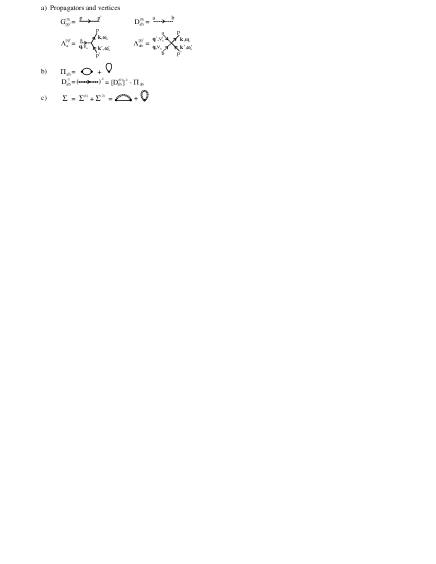
Figure 1: Summary of the Feynman rules. a) Solid lines represent the propagator $G^{(0)}$ (eq. (3)). Dashed lines represent the $8\times 8$ boson propagator $D^{(0)}$ (eq. (14)) for the $8$-component field $\delta X^{a}$. $\Lambda^{pp^{\prime}}_{a}$ and $\Lambda^{pp^{\prime}}_{ab}$ represent the interaction between two fermions $f_{p}$ and one or two bosons $\delta X^{a}$ respectively. b) Irreducible boson self-energy $\Pi_{ab}$. Double dashed lines correspond to a dressed boson propagators. c) Contributions to the electron self-energy $\Sigma({\bf k},\omega)$ in ${\cal O}(1/N)$.

The mean-field values $r_{0}$ and $\Delta$ must be determined by minimizing the leading order theory. From the completeness conditionfoussats06 , $\hat{X}^{00}+\sum_{p}\hat{X}^{pp}=\frac{N}{2}$, $r_{0}$ is equal to $x/2$ where $x$ is the doping away from half-filling. On the other hand, the expression for $\Delta$ is

$${}\Delta=\frac{J}{2N_{s}}\frac{1}{3}\sum_{k\eta}\cos(k_{\eta})n_{F}(E_{k})\;,$$ (5)

where $n_{F}$ is the Fermi function and $N_{s}$ is the number of lattice sites. For a given doping $x$; $\mu$ and $\Delta$ must be determined self-consistently from $(1-x)=\frac{2}{N_{s}}\sum_{k}n_{F}(E_{k})$ and eq. (5). $k_{\eta}$ is the proyection of ${\bf k}$ over the different bond directions ${\eta}_{1}=(1,0)$, ${\eta}_{2}=(\frac{1}{2},\frac{\sqrt{3}}{2})$ and ${\eta}_{3}=(-\frac{1}{2},\frac{\sqrt{3}}{2})$ of the triangular lattice.

We associate with the eight component boson field $\delta X^{a}=(\delta R\;,\;\delta{\lambda},\;r^{{\eta}_{1}},\;r^{{\eta}_{2}},\;r^{{\eta}_{3}},\;A^{{\eta}_{1}},\;A^{{\eta}_{2}},\;A^{{\eta}_{3}})$, the inverse of the propagator, connecting two generic components a and b (dashed line in Fig. 1),

$$D^{-1}_{(0)ab}({\mathbf{q}},\nu_{n})=N\left(\begin{array}[]{cccccccc}\gamma_{q}&x/2&0&0&0&0&0&0\\ x/2&0&0&0&0&0&0&0\\ 0&0&\frac{4}{J}\Delta^{2}&0&0&0&0&0\\ 0&0&0&\frac{4}{J}\Delta^{2}&0&0&0&0\\ 0&0&0&0&\frac{4}{J}\Delta^{2}&0&0&0\\ 0&0&0&0&0&\frac{4}{J}\Delta^{2}&0&0\\ 0&0&0&0&0&0&\frac{4}{J}\Delta^{2}&0\\ 0&0&0&0&0&0&0&\frac{4}{J}\Delta^{2}\end{array}\right),$$ (14)

where $\gamma_{q}=(2V-J)(x/2)^{2}\;\sum_{\eta}\cos k_{\eta}$ aclara1 and the indices $a$, $b$ run from 1 to 8. ${\bf q}$ and $\nu_{n}$ are the momentum and the Bose Matsubara frequency of the boson field, respectively.

The first component $\delta R$ of the $\delta X^{a}$ field is connected with charge fluctuations via $\hat{X}^{00}_{i}=Nr_{0}(1+\delta R_{i})$, where $\hat{X}^{00}_{i}$ is the Hubbard operator associated with the number of vacancies at site $i$. $\delta\lambda$ is the fluctuation of the Lagrange multiplier $\lambda_{i}$ associated with the completness condition. $r_{i}^{\eta}$ and $A_{i}^{\eta}$ correspond, respectively, to the amplitude and the phase fluctuation of the bond variable $\Delta_{i}^{\eta}=\Delta\,(1+r_{i}^{\eta}+i\,A_{i}^{\eta})$.

Fermions $f_{p}$ interact with the boson $\delta X^{a}$ via three and four leg vertices, namely $\Lambda^{pp^{\prime}}_{a}$ and $\Lambda^{pp^{\prime}}_{ab}$ respectively. The explicit expressions for these vertices can be found in Ref. [foussats06, ].

Each vertex conserves momentum and energy and they are of ${\cal O}(1)$. In each diagram there is a minus sign for each fermion loop and a topological factor.

The bare boson propagator $D_{(0)ab}$ (the inverse of eq. (14)) is ${\cal O}(1/N)$. From the Dyson equation, $D_{ab}^{-1}=D_{(0)ab}^{-1}-\Pi_{ab}$, the dressed components $D_{ab}$ (double dashed line in Fig. 1b) of the boson propagator can be found after the evaluation of the $8\times 8$ boson self-energy matrix $\Pi_{ab}$. Using the Feynman rules, $\Pi_{ab}$ can be evaluated through the diagrams of Fig.1b as shown in Ref. [foussats06, ].

This formalism is used here for calculating self-energies and one-particle spectral functionsbejas06 . The Green’s function (3) corresponds to the $N$-infinite propagator which includes no dynamical corrections; these appear at higher order in the $1/N$ expansion. Using the Feynman rules, the total self-energy in ${\cal O}(1/N)$ is obtained adding the contribution of the two diagrams shown in Fig. 1c.

After performing the Matsubara sum and the analytical continuation $i\omega_{n}=\omega+i\xi$, the imaginary part of $\Sigma$ is

$$Im\,\Sigma({\mathbf{k}},\omega) = \frac{1}{2N_{s}}\sum_{{\mathbf{q}}}h_{a}(k,q,\omega-E_{{k-q}})$$ (15)

$$B^{ab}({\mathbf{q}},\omega-E_{{k-q}})\;h_{b}(k,q,\omega-E_{{k-q}})$$

$$\times[n_{F}(-E_{k-q})+n_{B}(\omega-E_{{k-q}})]$$

where $n_{B}$ is the Bose factor, $B_{ab}$ is

$$B^{ab}({\mathbf{q}},\nu)=-2\lim_{\eta\rightarrow 0}\;Im\,[D_{ab}({\mathbf{q}},i\nu_{n}\rightarrow\nu+i\eta)].$$ (16)

and the 8-component vector aclara2 $h_{a}(k,q,\nu)$ is

$$h_{a}(k,q,\nu) = \left(\frac{2E_{k-q}+\nu+2\mu}{2}+2\Delta\sum_{\eta}\cos(k_{\eta}-\frac{q_{\eta}}{2})\cos(\frac{q_{\eta}}{2});1;-2\Delta\;\cos(k_{{\eta}_{1}}-\frac{q_{{\eta}_{1}}}{2});-2\Delta\;\cos(k_{{\eta}_{2}}-\frac{q_{{\eta}_{2}}}{2});\right.$$ (17)

$$\left.-2\Delta\;\cos(k_{{\eta}_{3}}-\frac{q_{{\eta}_{3}}}{2});2\Delta\;\sin(k_{{\eta}_{1}}-\frac{q_{{\eta}_{1}}}{2});2\Delta\;\sin(k_{{\eta}_{2}}-\frac{q_{{\eta}_{2}}}{2});2\Delta\;\sin(k_{{\eta}_{3}}-\frac{q_{{\eta}_{3}}}{2})\right)\;.$$

It is interesting to show $Im\,\Sigma$ expliciting the terms $B_{RR}$, $B_{\lambda R}$ and $B_{\lambda\lambda}$:

$$Im\,\Sigma({\mathbf{k}},\omega) = \frac{1}{2N_{s}}\sum_{{\mathbf{q}}}\left\{\Omega^{2}\;B^{RR}({\mathbf{q}},\omega-E_{{k-q}})\right.$$

$$+\;2\;\Omega\;B^{\lambda R}({\mathbf{q}},\omega-E_{{k-q}})+\left.B^{\lambda\lambda}({\mathbf{q}},\omega-E_{{k-q}})\right\}$$

$$\times\left[n_{F}(-E_{k-q})+n_{B}(\omega-E_{{k-q}})\right]+f({\bf k},\omega)\;,$$

where $\Omega=(E_{k-q}+\omega+2\mu)/2+2\Delta\sum_{\eta}\cos(k_{\eta}-q_{\eta}/2)\cos(q_{\eta}/2)$. In the function $f({\bf k},\omega)$ the other terms of eq. (15) have been included. After performing numerical calculations for the parameters used in the present paper, $f({\bf k},\omega)$ results at least an order of magnitud lower than the other terms of eq. (II).

Using the Kramers-Kronig relations, $Re\,\Sigma({{\bf{k}}},\omega)$ can be determined from $Im\,\Sigma({{\bf{k}}},\omega)$, eq. (15) and the spectral function $A({\bf k},\omega)=-\frac{1}{\pi}Im\,G({\bf k},\omega)$ can be computed as

$$A({\bf k},\omega)=-\frac{1}{\pi}\frac{Im\,\Sigma({\bf k},\omega)}{[\omega-E_{\bf k}-Re\,\Sigma({\bf k},\omega)]^{2}+[Im\,\Sigma({\bf k},\omega)]^{2}}$$

Notice that the self-energy is calculated using the propagator $G({\bf k},\omega)$ for the X-operators, that are proportional to the fermionic $f$-operators, which cannot be related to usual fermions.

III Charge density wave instabilities

The inclusion of a nearest neighbors Coulomb repulsion $V$ favors a charge density wave (CDW) state. In this section we will discuss the charge instabilityfoussats06 which will be of interest for analysing self-energy corrections.

The charge-charge correlation function $\chi^{c}_{ij}$ can be written as foussats02 ; gehlhoff95

$$\chi^{c}_{ij}(\tau)=\frac{1}{N}\sum_{pq}<T_{\tau}X_{i}^{pp}(\tau)X_{j}^{qq}(0)>\;.$$ (20)

Using the completeness condition and the relation between $\hat{X}^{00}_{i}$ and $\delta R_{i}$ ($\hat{X}^{00}=Nr_{0}(1+\delta R_{i})$), in Fourier space,

$$\chi^{c}({\bf{q}},\omega)=-N\left(\frac{x}{2}\right)^{2}D_{RR}({\bf{q}},\omega)\;.$$ (21)

Then, in our formulation, the charge correlation function is proportional to the component $(1,1)$ (also called $D_{RR}$) of the dressed boson propagator $D_{ab}$.

The divergence of the static charge susceptibility (21) marks the onset for the CDW instability. For the triangular lattice the charge susceptibility diverges at ${\bf Q}=(4/3\pi,0)$ for $V=V_{c}$. This new phase is called $\sqrt{3}\times\sqrt{3}$ CDW motrunich04 ; foussats05 ; foussats06 . In what follows all energies ($V$, $J$, etc.) are given in units of $t$.

Figure 2 shows the phase diagram in the $V_{c}-x$ plane at temperature $T=0$. As in Ref. [foussats06, ], we will use $J=0.2$. The different phases are the homogeneous Fermi liquid (HFL), the $\sqrt{3}\times\sqrt{3}$ CDW, the bond-order phase (BOP), and a phase separation (PS) region. However, in this paper we focus only on the proximity to the HFL-CDW transition (see Ref. [foussats06, ] for details about the BOP and PS phases). For the large doping studied here results are very robust against different $J$ values as long as they are not considered to be unphysically large. Only for unphysical large values $J\sim 1$, the BOP and PS regions approach the doping levels considered here. But for $J<0.5$, a value well beyond the physical ones in e.g. cobaltates, the HFL and CDW phases are well defined beyond $x\sim 0.15$.

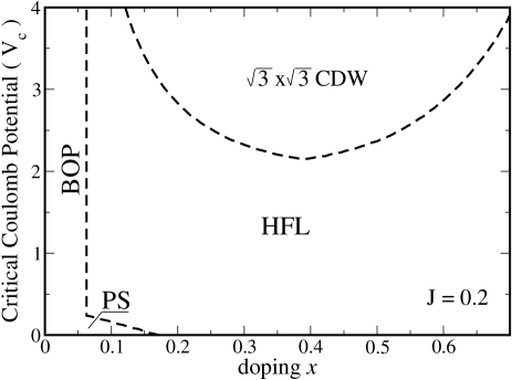
Figure 2: Phase diagram in the $V_{c}-x$ plane for $J=0.2$. The homogeneous Fermi liquid (HFL) is unstable against phase separation (PS), bond order phase (BOP) and the $\sqrt{3}\times\sqrt{3}$ CDW. BOP and PS are discussed in Ref. [foussats06, ] and are presented here only for a complete description of the phase diagram. For a given doping $x$ the static charge susceptibility diverges at $V_{c}$ where the onset to a $\sqrt{3}\times\sqrt{3}$ CDW occurs.

Next, we study the charge dynamics on approaching the $\sqrt{3}\times\sqrt{3}$ CDW from the HFL. In Figs. 3 and 4 results for $Im\,\chi^{c}({\bf Q},\omega)$ are presented for two commensurate doping values $x=2/3$ and $x=1/3$, respectively. The momentum was fixed at ${\bf Q}=(4/3\pi,0)$.

For $x=2/3$ (Fig. 3) and for $V=0$ (solid line), we clearly see a collective peak at $\omega\sim 3.1t$ at the top of the particle-hole continuum (inset). With increasing $V$ the collective peak becomes soft and accumulates spectral weight as shown for $V=2.0$ (dotted line), $V=3.0$ (dashed line) and $V=3.2$ (dotted dashed line). At $V=V_{c}\sim 3.6$, the collective peak reaches zero frequency condensing a $\sqrt{3}\times\sqrt{3}$ CDW phase. Therefore, the charge instability can clearly be seen as the softening of the collective charge mode. For $x=2/3$, charge dynamics is very similar to the case of the square lattice at one quarter filling where the softening of the charge mode was obtained and discussed in the context of organic materialsmerino03 .

Figure 3: (color online) $Im\,\chi_{c}({\bf Q},\omega)$ for $x=2/3$, $J=0.2$ and for different values of $V$ approaching $V_{c}\sim 3.6$. ${\bf Q}=(4\pi/3,0)$, where the static charge susceptibility diverges. For $V=0$, the collective charge peak is formed at the top of the particle-hole continuum (inset). With increasing $V$ the collective peak becomes soft and emerges from the bottom of the continuum accumulating spectral weight. For $V=V_{c}\sim 3.6$ this soft collective peak reaches $\omega=0$ freezing the $\sqrt{3}\times\sqrt{3}$ CDW phase.

For $x=1/3$ (Fig. 4), the situation is somewhat different. For $V=0$ (solid line) the collective peak is located at $\omega\sim 2.2t$, above the particle-hole continuum. With increasing $V$ towards $V_{c}\sim 2.35$, a transfer of spectral weight takes place over a large energy range since the collective charge mode spreads over the particle-hole continuum.

The reason for the different behavior between $x=1/3$ and $x=2/3$ is due to the form of the particle-hole continuum for each doping (insets in Figs. 3 and 4). For $x=2/3$ there is a gap at low energy, since for $x=2/3$ $2{\bf k_{F}}<{\bf Q}$, and particle-hole transitions are not possible for $\omega<1$. For $V=0$ the collective peak is formed at the top of this continuum (Fig. 3 solid line). When V increases, the collective peak softens (Fig. 3) and for large $V$, near $V_{c}$, emerges from the continuum until it reaches $\omega=0$ exactly at $V_{c}$ (see for instance solid and dashed lines in Fig. 3). In contrast, for $x=1/3$ there is no gap in the particle-hole continuum (inset Fig. 4). When the collective mode enters the particle-hole continuum, a spread of spectral weight over a wide range takes place, and for $V$ approaching $V_{c}$, it emerges from the continuum as a resonance.

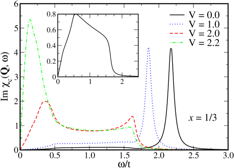
Figure 4: (color online) Similar to Fig. 3 for $x=1/3$ ($V_{c}\sim 2.35$). Notice the different behaviour with respect to $x=2/3$ (see text). Inset: particle-hole continuum.

Before closing the section, we present in Fig. 5 the $T$-$V$ phase diagram for $x=1/3$ and $x=2/3$. $T_{CO}$ is the temperature for charge ordering. The obtained reentrant behavior of the charge order transition was also predicted by several calculations pietig99 ; hellberg01 ; hoang02 ; merino06 ; merino01 . Recently, it was proposed that a reentrant behavior near charge order is necessary for describing anomalous optical features in $1/4$-filling organic materialsmerino06 (see Sec. V for more details).

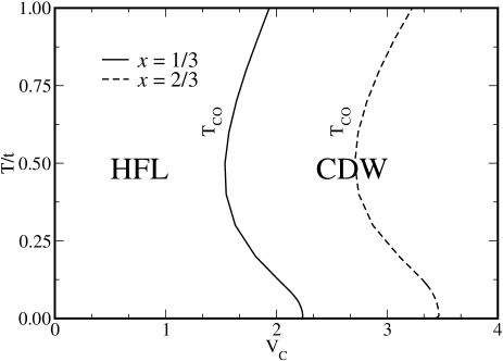
Figure 5: $T$-$V$ phase diagram for $x=1/3$ (solid line) and $x=2/3$ (dashed line).

In the next section, we will study self-energy corrections approaching the $\sqrt{3}\times\sqrt{3}$ CDW phase and discuss the role played by the soft modes mentioned above.

IV One-particle properties beyond mean-field level

IV.1 Quasiparticle weight

The self-energy allows the calculation of the quasiparticle (QP) weight $Z=1/(1-\frac{\partial\Sigma}{\partial\omega})$ at the Fermi level. In Fig. 6, the QP weight is plotted as a function of $V$ for $x=1/3$ (solid line) and for $x=2/3$ (dashed line). The Fermi vectors are located in the $\Gamma-K$ direction of the Brillouin zone for both, $x=1/3$ and $x=2/3$. As we will discuss below, our self-energy is very isotropic on the Fermi surface (FS) such that Fig. 6 is representative for all points on the FS. In both cases, when $V$ approaches the corresponding $V_{c}$, the QP weight decreases suggesting that it tends to zero at $V_{c}$ (see dotted arrows). Below, the analysis of spectral weight transfer at small energy will give additional support for this result.

The behavior presented in Fig. 6 indicates the breakdown of the Fermi liquid (FL) at $V_{c}$. Therefore, our calculation suggests a metal insulator transition where a rather isotropic gap should exists for $V>V_{c}$. Our observation is based on the fact that for $V<V_{c}$ the QP weight $Z$ is very isotropic on the FS such that the FL breaks down for all points on the FS.

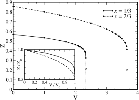
Figure 6: The quasiparticle weight $Z$ for $J=0.2$ evaluated on the Fermi surface as a function of $V$ for $x=1/3$ (solid line) and $x=2/3$ (dashed line). With increasing $V$ both curves show that, first, $Z$ decreases slowly and, it drops to zero close to $V_{c}$ ($Z\rightarrow 0$ for $V\rightarrow V_{c}$). Dotted lines are guides for the eyes which show the mentioned tendency (see text for discussions). For $V=0$ the quasiparticle weight for $x=1/3$ is smaller than for $x=2/3$ which means that correlations are stronger for small than for large $x$. Inset: The QP weight divided by the QP weight at $V=0$ ($Z/Z_{0}$) versus $V/V_{c}$ for $x=1/3$ (solid line) and $x=2/3$ (dashed line). With increasing $V$, the decreasing of $Z$ is somewhat faster for $x=2/3$ than for $x=1/3$. See text for discussions.

In both curves, when $V$ increases the QP weight decreases, first relatively slowly, and then drops to zero close to $V_{c}$. Therefore, near the CDW instability the QP carries very small weight making the electronic dynamics very incoherent. To clarify this point better we will present below results for the spectral functions.

The QP weight for $V=0$ (far from the CDW instability) is already reduced from one. This reduction is not related to the CDW instability but it is due to electronic correlation effects which our method is able to capture in the pure $t$-$J$ model. In fact, Fig. 6 shows that the QP weight for $x=1/3$ is smaller than for $x=2/3$, as one expects, since correlation effects should be weaker for a dilute system. For $x\rightarrow 1$ our method predicts $Z\rightarrow 1$ which corresponds to the uncorrelated limit (empty band). On the other hand, in both cases, $Z$ strongly decreases on approaching the charge order intstability.

IV.2 Self-energy

The discussion above indicates that the HFL is strongly modified near the CDW instability, where the carriers are renormalized by interacting with soft charge fluctuations. In order to discuss this point in detail, we will present results for the self-energy $\Sigma({\bf k},\omega)$.

In Fig. 7, self-energy results at ${\bf k}={\bf k_{F}}$ are presented for $x=1/3$ and several values of $V$ approaching $V_{c}$. Panel (a) shows $-Im\,\Sigma$ as a function of frequency. As discussed in Ref. [bejas06, ], for $V=0$, $Im\,\Sigma$ is strongly asymmetric with respect to $\omega=0$ and behaves as $\sim\omega^{2}$ at small $\omega$’s. The self-energy presents large contributions at large energy of the order of $t$ below the Fermi energy. With increasing $V$ a redistribution of the weight takes place and $Im\,\Sigma$ develops structures at energies close to but above the Fermi energy. As $Im\,\Sigma$ and $Re\,\Sigma$ are related to each other by a Kramers Kronig transformation, the changes in $Im\,\Sigma$ are reflected in $Re\,\Sigma$ (panel (b)). For instance the slope of $Re\,\Sigma$ at $\omega=0$ increases with increasing $V$ leading to a decrease of the QP weight discussed in Fig. 6. The inset in panel (b) shows this behavior in a smaller scale near $\omega=0$. While for $V\leq 2.2$ a gradual change in the slope is observed, very close to $V_{c}$, a stronger increase is observed, as shown by the thick solid line corresponding to $V=2.34$.

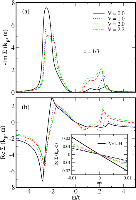
Figure 7: (color online) Self-energy $\Sigma({\bf k_{F}},\omega)$ for $x=1/3$ and $J=0.2$ for several values of $V$ approaching $V_{c}\sim 2.35$. (a) $-Im\,\Sigma({\bf k_{F}},\omega)$ versus $\omega$. It presents large structures at energies of the order of $t$ and shows a $\sim\omega^{2}$ behavior around $\omega=0$. With increasing $V$ a redistribution of the weight takes place. (b) $Re\,\Sigma({\bf k_{F}},\omega)$ versus $\omega$ for the same values of $V$ as in panel (a). Inset shows that, with increasing $V$, the slope of $Re\,\Sigma$ near $\omega=0$ increases leading to a decrease of the quasiparticle weight.

IV.3 Spectral functions and total density of states

Using $Im\,\Sigma$ and $Re\,\Sigma$, the spectral function $A({\bf k},\omega)$ can be calculated as usual. Figure 8 presents results for $A({\bf k}_{F},\omega)$ for several values of $V$. The peak at $\omega=0$ corresponds to the QP while the other features, for instance at $\omega\sim-3t$ and $\omega\sim 2.5t$, are of incoherent character. For $V=0$ (solid line) the QP weight is $Z\sim 0.56$ (Fig. 6) and the incoherent structure is mainly concentrated in the pronounced feature at $\omega\sim-3.5t$. Increasing $V$ up to $V=2.2$ (dotted dashed line) the QP weight decreases ($Z\sim 0.42$) and, at the same time, spectral weight appears at $\omega\sim 0.5t-2.5t$ (Fig. 8). In addition, with increasing $V$, the incoherent structure at $\omega\sim-3.5t$ moves to the right while loses some weight.

In Fig. 8 it was assumed, supported by the Luttinger theorem, that ${\bf k_{F}}$ does not change with the interaction $V$. On the other hand, if we wish to compare with $ARPES$ experiments (see Sec. V), our input is a tight binding dispersion which reproduces the measured FS which already contains the interactions. The comparison between our approach and Lanczos diagonalization presented in Ref. [bejas06, ] gives an additional support fort this assumption (see also Ref. [merino03, ]).

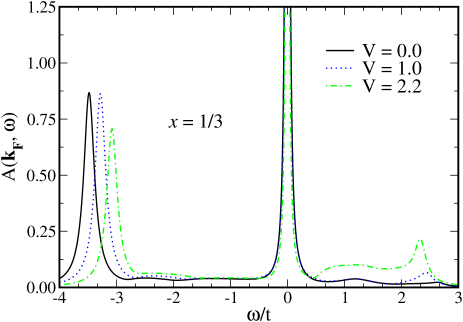
Figure 8: (color online) Spectral function $A({\bf k}_{F},\omega)$ versus $\omega$ for $J=0.2$ and several values of $V$ approaching $V_{c}\sim 2.35$. For $V=0$ (solid line), pure $t$-$J$ model correlation effects leads to a quasiparticle peak with reduced weight $Z\sim 0.56$ and incoherent structures at positive and negative energies. With increasing $V$, while the QP weight decreases (Fig. 6), weight is transfered to the range $\omega\sim 0.5t-2.5t$.

IV.4 Physical origin of the self-energy renormalizations: $\alpha^{2}F(\omega)$

In the following we discuss the interaction of the bosonic excitations described by $D_{RR}$ (see eq. (21)) with electrons that lead to the self-energy renormalizations discussed in the previous section. In many body theory mahan the quantity which contains this information is $\alpha^{2}F(\omega)$ where, $F(\omega)$ is the density of states of a boson which interacts with the fermions with strength $\alpha$. At $T=0$ norman06 ,

$$Im\,\Sigma(\omega)=\int_{0}^{\omega}d\Omega\;\alpha^{2}F(\Omega)\;,$$ (22)

i.e. $\alpha^{2}F(\omega)=\partial Im\,\Sigma(\omega)/\partial\omega$. In eq. (22) the average over all momentum transfer ${\bf q}={\bf k}_{1}-{\bf k}_{2}$, where ${\bf k}_{1}$ and ${\bf k}_{2}$ are two Fermi vectors, is assumed mahan .

In Fig. 9 we have plotted $\alpha^{2}F$ for the same values of $V$ as in Fig. 7. As we mentioned above, our self-energy is very isotropic on the FS such that $\alpha^{2}F$ evaluated at ${\bf k_{F}}$ is representative for the average over the FS.

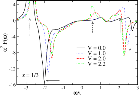
Figure 9: (color online) $\alpha^{2}F(\omega)$ for the same values of $V$ as in Fig. 7. The features marked with solid arrows are related with collective charge fluctuations which become soft with increasing $V$ and, at the same time, $\alpha^{2}F(\omega)$ acquires structures at low energies (dashed arrow) which lead to the decreasing of $Z$ (see text).

Let us discuss first the case for $V=0$ (solid line). We can see two structures, at $\omega\sim-2t$ and $\omega\sim 2t$ (solid arrows) which are related with collective charge excitations (see below). The features at $\omega\sim-3t$ and $\omega\sim 2.5t$ (dotted arrows) are due to the fact that $Im\,\Sigma$ (Fig. 7) is concentrated in a finite range of energy (between the borders $\sim-4t$ and $\sim 3t$) so that, when performing the derivative $\partial Im\,\Sigma(\omega)/\partial\omega$ to obtain $\alpha^{2}F(\omega)$, these two features are created at these two borders. In Fig. 10 we have plotted the average of the $Im\,\chi^{c}({\bf q},\omega)$ for all ${\bf q}$ such that ${\bf q}={\bf k_{1}}-{\bf k_{2}}$ where ${\bf k_{1}}$ and ${\bf k_{2}}$ are two Fermi vectors. For $V=0$ (solid line), the well defined peaks (solid arrows) at $\omega\sim-2t$ and $2t$ are due to collective charge excitations while tails are due to the particle-hole continuum (see solid line in Fig. 4). Clearly, the two structures marked with solid arrows in Fig. 9 are correlated with the corresponding ones in Fig. 10 showing that these structures in $\alpha^{2}F$ are related to collective charge fluctuations while tails, are due to the particle-hole continuum. The reason why $\alpha^{2}F(\omega)$ does not trace exactly the average of the charge correlations of Fig. 10 is the following. $\alpha^{2}F$ contains information of both, the density of states of the interacting boson and its coupling with fermions but, in a mixed form. For instance, the only way that $\alpha^{2}F$ follows exactly the same shape of the boson density of states occurs if the coupling does not depend on $\omega$ or momentum. This condition is not satisfied in our case which can be seen by looking at the expression (II) for $Im\,\Sigma$. On the other hand, only in the first term of eq. (II) the charge-charge correlation is explicitly present. The other terms which contain $D_{\lambda R}$ and $D_{\lambda\lambda}$ are proper of our method, and they are due to the nondouble occupancy constraint.

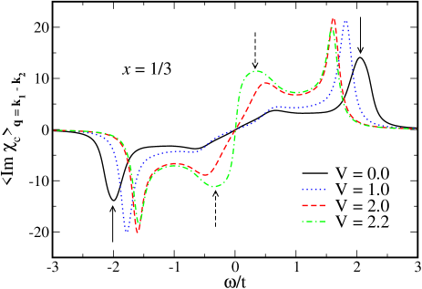
Figure 10: (color online) Average of $Im\,\chi_{c}({\bf q},\omega)$ for all ${\bf q}$ such that ${\bf q}={\bf k_{1}}-{\bf k_{2}}$ with ${\bf k}_{1}$ and ${\bf k}_{1}$ on the FS. With increasing $V$, the collective charge peaks (solid arrows) become soft and at the same time a soft dynamics (dashed arrows) appears at low energies. The close correlation between these features and those discussed in Fig. 9 shows that the charge dynamics is the main cause for the reduction of $Z$ near charge order.

With increasing $V$, the features marked with solid arrows in Fig. 9 become soft and, at the same time, spectral weight appears at lower energies (dashed arrows). This behavior is clearly correlated with that depicted in Fig. 10 which shows the soft charge dynamics discussed in Sec. III (see Fig. 4).

It is well known mahan that

$$-\frac{\partial Re\,\Sigma}{\partial\omega}=\int d\omega\frac{\alpha^{2}F(\omega)}{\omega}\;.$$ (23)

Therefore, the presence of low energy excitations in $\alpha^{2}F$ leads to an increase of $\partial Re\,\Sigma/\partial\omega$ and hence, to a decrease of the QP weight $Z$. Notice that near $V_{c}$, $\alpha^{2}F(\omega)$ shows, besides the low energy features, structure at high energy in agreement with the behavior presented by charge correlations (Fig. 4 and Fig. 10). The fact that not all the spectral weight is concentrated at low energy is the cause for the slow decrease of $Z$. The inset of Fig. 6 shows that $Z$ decreases somewhat faster for $x=2/3$ than for $x=1/3$ which is consistent with the fact that softening of the charge collective mode is more clear for $x=2/3$ (see Figs. 3 and 4).

To conclude, we think that we have given clear arguments which show that the charge collective soft modes near the CDW are responsible for the incoherent motion of the carriers near charge ordering. In addition, the charge soft modes reach $\omega=0$ at $V_{c}$ which means that $-\partial Re\,\Sigma/\partial\omega\rightarrow\infty$ (eq. 23) and then $Z\rightarrow 0$ as indicated in Fig. 6.

IV.5 E-k structures

When discussing the spectral functions we have shown the presence of coherent QP peaks and incoherent structures. In Fig. 11 we show the energy position of the main visible structures for $V=0$ and $V=2.2$ at $x=1/3$ along the main directions of the Brillouin zone (inset in Fig. 11). Dashed lines mark the spectral functions at ${\bf k_{F}}$. For $V=0$ (panel (a)), we can see that the QP band (near the FS) and a dispersing incoherent band at $\omega\sim-3t$ dominate the spectra.

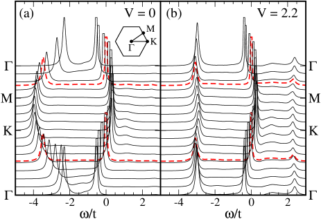
Figure 11: (color online) Spectral functions at $x=1/3$ in the main directions of the Brillouin zone for (a) $V=0$ and (b) $V=2.2$. The peak near $\omega=0$ is the coherent quasiparticle peak and the other structures are of incoherent character. For $V=2.2$ the coherent QP band becomes flatter and an incoherent band appears in the energy range $\omega\sim 0.5t-2.5t$. The QP peak has been cut for clarity purposes.

When $V$ increases to $V=2.2$ (panel (b)) the QP coherent band becomes less dispersing consistently with the reduction of the QP weight. The incoherent band at negative $\omega$ becomes also less dispersing. Interestingly, an incoherent band is formed in the region $\sim 0.5t-2.5t$. Notice that no kink is showed by the coherent QP band. This is because the kink, if it exist, should be located at energies of the order of the interacting boson (which in this case is related to the soft mode) and, at $V=2.2$, it is still located at energies of $\sim 0.2t$ (Fig. 4) which is of the order of the QP bottom energy.

V Comparison with cobaltates

In previous sections we have discused one-particle spectral predictions of the large-$N$ approach for the $t$-$J$-$V$ model on the triangular lattice without making emphasis on any particular system. In this section we will discuss previous results and their possible contact with cobaltates. First principle calculations in cobaltates singh03 predict, besides a large hole Fermi surface around $\Gamma$, the existence of six small pockets near the corners of the Brillouin zone. Until now, all ARPES experiments both, in hydratedqian06_97 ; shimojima06 and unhydrated cobaltates qian06 ; hasan04 ; yang04 ; dqian06p ; mhasan06p ; kuprin06 ; yang05 do not show the presence of these small pockets. The absence of pockets in ARPES can be understood by the renormalization of the bands due to strong electronic correlations zhou05 . In fact, a reduction of the bandwidth and large electronic effective masses are observed in ARPES dqian06p ; mhasan06p . In addition, in a very recent work vaulx07 it was pointed out that cobaltates are close to a Mott insulator in the limit $x\rightarrow 0$

Following these ideas, a one-band $t$-$J$ model on the triangular lattice, as proposed in the present paper, seems to be appropriated for studying cobaltates. For this purpose, $\tilde{c}^{\dagger}_{i\sigma}$ and $\tilde{c}_{i\sigma}$ in eq. (1) must be associated with the creation and destruction of holes respectively, as in Refs. [motrunich04, ; foussats05, ; motrunich03, ]. Then, in this context, the doping $x$ is the electron doping away from half-filling. Considering the bare hoping $t\sim 150meV$singh00 and $U_{dd}\sim 3.0-5.5eV$ chainani04 we obtain $J/t\sim 0.1-0.2$, similarly to the value used in previous sections. In addition, we will mainly focus the comparison with our results for $x=1/3$, which is close to the doping where the maximum superconducting critical temperature $T_{c}$ is found in cobaltates. For $x<0.5$ our results predict a Pauli paramagnet as observed in cobaltates. On the other hand, as cobaltates exhibit a Curie-Weiss behavior in the region $x>0.5$, we will not relate our results in $x=2/3$ with experiments. However, it is important to mention that it is not clear if this Curie-Weiss behavior is due to the fact that electronic correlations are more important for $x>0.5$ or other effects, as for instance $Na$ order, are predominant (see Ref.[schulze07, ] and references their in).

According to results in previous sections we have two factors which reduce the Fermi velocities from the bare one. The first one occurs already at mean field level where the effective hopping is $(x/2)t$ instead of $t$. The second one, which is obtained only after evaluating fluctuations beyond mean field is the quasiparticle weight $Z$. Therefore, the Fermi velocity is $v_{F}\sim(x/2)\;Z\;v_{F}^{LDA}$ where $v_{F}^{LDA}$ is the bare Fermi velocity extracted from LDA calculations. Using the parameters for cobaltates and our results for $x=1/3$ up to $0.9V_{c}$ we obtain $v_{F}\sim 0.21eV\AA$. This value is close to the value $v_{F}=(0.30\pm 0.05)eV\AA$ found in Refs. [mhasan06p, ; dqian06p, ]. This small value was consideredmhasan06p as an indication for the presence of strong correlations and, the ratio between $T_{c}$ and the Fermi velocity was found to be close to the same ratio for cuprates. In agreement with these experiments, our calculation shows also a rather isotropic Fermi velocity over the BZ (see Fig. 11). Another interesting and qualitative agreement between experiments and our finding is the following: in Ref. [mhasan06p, ] it was found that the scattering rate behaves as $\sim\omega^{2}$ near the Fermi surface which agrees with results in panel (a) of Fig. 7.

In our previous papersfoussats05 ; foussats06 , for describing superconductivity in cobaltates we proposed, like other works motrunich04 ; motrunich03 ; tanaka04 , that the system is close to $\sqrt{3}\times\sqrt{3}$ charge order. The charge order scenario is supported by some experimentsshimojima05 ; lemmens05 ; qian06 . In addition, ARPES experiments dqian06p show a Fermi surface topology, very close to our FS, which favors charge instabilities. We have proposed that the interplay between electronic correlations and phonons are relevant for describing superconductivity with triplet NNN-$f$ pairing as predicted by some experiments fujimoto04 ; kato06 ; ihara05 ; kanigel04 ; higemoto04 . For this scenario we need that, with increasing water content, the system comes closer to charge ordering. Recent ARPES experimentsqian06_97 ; shimojima06 have shown that the Fermi velocity do not vary very much with the water content. These experiments seem to be in contradiction with our result of Fig. 11 where it is possible to see that very close to the charge instability the band dispersion becomes flat. However, we think that it is possible that for the water content reached in the experiments the system is still far from the static charge order state i.e., in the regime where $Z$ does not change very much. This could explain the reason why NMRmukhamedshin05 does not show the charge order because it is fluctuating faster than the time-scale accessible by NMR. We remember that for obtaining a robust description of superconductivity we do not need to place the system very close to the charge order being enough a $V\sim 80-90\%V_{c}$ foussats05 ; foussats06 . However, for $V>0.9V_{c}$, $Z$ is strongly reduced and two competing effects can be expected. From one side, the decreasing of $Z$ may cause an increasing of the electronic density of states and then, a reinforcement of superconductivity. On the other side, when $Z$ decreases the quasiparticle losses coherence thus, superconductivity may be diminished. A careful study of this competition requires the calculation of superconducting pairing in ${\cal O}(1/N^{2})$.

It is interesting to compare our results with a very recent ARPES experiment on a series of $Bi$ cobaltates brouet . These compounds contain the same triangular $Co$ planes as $Na$ cobaltates. Besides a flat QP band with similar Fermi velocity as in $Na$ cobaltates, incoherent features were observed at high energy in the $Bi$ cobaltates. In that paper it was discused that these incoherent features are created with weight transfered from the QP band, a mechanism similar to that discussed in Sec. IV (notice the analogy, for instance, between Fig. 2 of Ref. [brouet, ] and our Fig. 11). On the other hand, the center of the incoherent band in Fig. 2 of Ref. [brouet, ] is at $\sim-0.5$ eV, close to the center of our incoherent band (Fig. 11) which, using $t=150$ meV is about $-0.45$ eV. Similar high energy features were recently observed in cuprates (see Ref. [brouet, ] and references their in) and, the present approach was used greco07 for discussing those features occuring in the overdoped side where, as mentioned before, our method is expected to be reliable.

Optical conductivity experiments hwang05 ; wu06 show a different behavior to usual metals where, besides a Drude peak at low energies, a broad absorption centered around $\sim 250$ meV is observed and interpreted as a pseudogapwu06 behavior. Similar features are observed in organic materials and discussed in term of the charge order proximity dressel03 . From our results in Fig. 8 we expect that, near the charge order, transitions from the Drude peak to the broad structure formed between $\sim 75-375$ meV (where we used $t=150$ meV) are possible leading to the optical absorption as in the experiments.

Recently, optical conductivity experiments in organic materials drichko06 have also shown an anomalous increasing of the effective mass with temperature. In Ref. [merino06, ], a reentrant behavior in the $T$-$V$ phase diagram, as the one discussed in our Fig. 5, was found to be responsible for the increase in effective mass. If for cobaltates $0.7V_{c}<V<V_{c}$, we think that an increase in effective mass with temperature can also be expected in these materials. From Fig. 5, depending on the value of $V$, the effective mass increase may occurs for $T<800$ K. It will be interesting to perform this kind of experiments.

VI Conclusion and discussions

In this paper, the $t$-$J$-$V$ model at finite density was studied on the triangular lattice. $V$ represents the Coulomb interaction between nearest neighbors and it is the parameter responsible for triggering a charge order phase for $V>V_{c}$. $V_{c}$ is the critical Coulomb repulsion whose numerical value depends on doping (Fig. 2). Studying charge correlation functions, it was shown that near $V_{c}$ charge dynamics becomes soft and, at $V=V_{c}$, charge modes collapse to zero frequency freezing a $\sqrt{3}\times\sqrt{3}$ CDW phase (Figs. 3 and 4).

By evaluating fluctuations beyond the mean field level, one-particle spectral properties were computed. Far away from charge ordering, i.e. for zero or small $V$, the QP weight $Z$ is reduced from one due to pure $t$-$J$ model correlations effects. With increasing $V$, $Z$ decreases slowly until $V\sim 90\%$ of $V_{c}$.  Beyond this value $Z$ decreases faster approaching zero at $V_{c}$ (Fig. 6). Therefore, near $V_{c}$ the electronic dynamics becomes very incoherent. For $V<V_{c}$, the scattering rate behaves as $Im\,\Sigma\sim\omega^{2}$ (Fig. 7(a)) which is characteristic for a Fermi liquid behavior. In addition, when the system approaches charge ordering, $Im\,\Sigma$ accumulates spectral weight at low energy. Due to this fact, the slope of $Re\,\Sigma$ at $\omega=0$ increases (Fig. 7(b)) leading to the decrease of $Z$ discussed above.

From $Im\,\Sigma$ and $Re\,\Sigma$ the spectral function $A(k,\omega)$ was calculated. With increasing $V$, approaching $V_{c}$, the most important changes are present at energies close but larger than the Fermi energy ($\omega=0$). While the weight of the QP peak decreases ($Z$ decreases), spectral weight appears at small positive energy in the range $\sim 0.5t-2.5t$ (Fig. 8).

The calculation of $\alpha^{2}F(\omega)$ allows to identify the excitations responsible for the self-energy effects. Computing $\alpha^{2}F(\omega)$ as a function of $V$ approaching $V_{c}$, it was shown that its behavior can be, without ambiguity, correlated with charge spectra (Figs. 9 and 10). Therefore, the charge soft modes, responsible for the charge instability, lead to an increase of $\alpha^{2}F$ at small frequencies with the corresponding decrease of $Z$.

In Sec. V, we mainly confronted our results with recent $ARPES$ experiments in cobaltates. We found our results to be in agreement with experiments presented in Refs. [dqian06p, ; mhasan06p, ; brouet, ].

Finally, we would like to point out that while our results were obtained for a purely 2D system, we expect only quantitative differences in our results when passing to a corresponding anisotropic 3D system, since we are dealing here with a spontaneous symmetry breaking of a discrete symmetry, as corresponds to a commensurate CDW. Certainly critical exponents may change, but they are beyond the scope of our treatment.

Acknowledgements A. G. thanks to M. Dressel, N. Drichko and J. Merino for interesting discussions.

References

- (1) P. W. Anderson, Science 235, 1196 (1987).
- (2) K. Takada et al., Nature 422, 53 (2003).
- (3) O. I. Motrunich and P. A. Lee, Phys. Rev. B 70, 024514 (2004).
- (4) Y. Tanaka, Y. Yanase, and M. Ogata, Jour. Phys. Soc. Jpn. 73, 319 (2004).
- (5) A. Foussats, A. Greco, M. Bejas, and A. Muramatsu, Phys. Rev. B 72, 020504(R) (2005).
- (6) A. Foussats, A. Greco, M. Bejas, and A. Muramatsu, J. Phys.: Condens. Matter 18, 11411 (2006).
- (7) T. Shimojima et al., Phys. Rev. B 71, 020505 (2005).
- (8) P. Lemmens et al., Phys. Rev. Lett. 96, 167204 (2006).
- (9) D. Qian et al., Phys. Rev. Lett. 96, 046407 (2006).
- (10) A. Foussats and A. Greco, Phys. Rev. B 65, 195107 (2002); A. Foussats and A. Greco, Phys. Rev. B 70, 205123 (2004).
- (11) M. Bejas, A. Greco and A. Foussats, Phys. Rev. B 73, 245104 (2006).
- (12) Z. Wang, Int. J. Mod. Phys. B 6, 155 (1992).
- (13) P. A. Lee, N. nagaosa, and X.-G. Wen, Rev. Mod. Phys. 78, 17 (2006).
- (14) J. Hubbard, Proc. R. Soc. London A 276, 238 (1963).
- (15) was corrected (a factor was removed) from previous versions.
- (16) A typing error in the second term of the first component of in Ref.[bejas06, ] was corrected now in eq.(17).
- (17) L. Gehlhoff and R. Zeyher, Phys. Rev. B 52, 4635 (1995).
- (18) J. Merino, A. Greco, R. H. McKenzie, and M. Calandra, Phys. Rev. B 68, 245121 (2003).
- (19) R. Pietig, R. Bulla and S. Blawid, Phys. Rev. Lett 82, 4046 (1999).
- (20) C. Stephen Hellberg, J. Appl. Phys. 89, 6627 (2001).
- (21) A. T. Hoang and P. Thalmeier, J. Phys.: Condens. Matter 14, 6639 (2002).
- (22) J. Merino, A. Greco, N. Drichko and M. Dressel, Phys. Rev. Lett. 96, 216402 (2006).
- (23) J. Merino and R. H. McKenzie, Phys. Rev. Lett. 87, 237002 (2001).
- (24) G. Mahan, Many-Particle Physics (Plenum Press, New York, 1981).
- (25) N. R. Norman and A. V. Chubukov, Phys. Rev. B 73, 140501(R) (2006).
- (26) D. J. Singh, Phys. Rev. B 68, 020503(R) (2003).
- (27) D. Qian et al., Phys. Rev. Lett. 97, 186405 (2006).
- (28) T. Shimojima et al., Phys. Rev. Lett. 97, 267003 (2006).
- (29) M. Z. Hasan et al., Phys. Rev. Lett. 92, 246402 (2004).
- (30) H. B. Yang et al., Phys. Rev. Lett. 92, 246403 (2004).
- (31) D. Qian et al., Phys. Rev. Lett. 96, 216405 (2006).
- (32) M. Z. Hasan, D. Qian, M. L. Foo and R. J. Cava, Annals of Physics 231, 1568 (2006).
- (33) A. P. Kuprin et al., J. Phys. Chem. of Solids 67, 235 (2006).
- (34) H. B. Yang et al., Phys. Rev. Lett. 95, 146401 (2005).
- (35) S. Zhou et al., Phys. Rev. Lett. 94, 206401 (2005).
- (36) C. de Vaulx et al., Phys. Rev. Lett. 98, 246402 (2007)
- (37) O. I. Motrunich and P. A. Lee, Phys. Rev. B 69, 214516 (2004).
- (38) D. J. Singh, Phys. Rev. B 61, 13397 (2000).
- (39) A. Chainani et al., Phys. Rev. B 69, 180508(R) (2004).
- (40) T. F. Schulze et al., arXiv:0707.1630.
- (41) T. Fujimoto et al., Phys. Rev. Lett. 92, 047004 (2004).
- (42) M. Kato et al., J. Phys.: Condens. Matter 18, 669 (2006).
- (43) Y. Ihara et al., J. Phys. Soc. Japan 75, 013708 (2006).
- (44) A. Kanigel et al., Phys. Rev. Lett. 92, 257007 (2004).
- (45) W. Higemoto et al., Phys. Rev. B 70, 134508 (2004).
- (46) I. Mukhamedshin, H. Alloul, G. Collin, and N. Blanchard, Phys. Rev. Lett. 94, 247602 (2005).
- (47) V. Brouet et al., arXiv:0706.3849.
- (48) A. Greco, Solid State Communications 142, 318 (2007). See also F. Tan, Y. Wan, and Q.-H. Wang, Phys. Rev. B 76, 054505 (2007) and F. Tan and Q.-H. Wang, arXiv:0709.3870 where, in spite of a different method was used, similar results were obtained.
- (49) J. Hwang, J. Yang, T. Timusk, and F. Chou, Phys. Rev. B 72, 024549 (2005).
- (50) D. Wu, J. L. Luo, and N. L. Wang, Phys. Rev. B 73, 014523 (2006).
- (51) M. Dressel, N. Drichko, J. Schlueter, and J. Merino, Phys. Rev. Lett. 90, 167002 (2003).
- (52) N. Drichko et al., Phys. Rev. B 74, 235121 (2006).