Drift instabilities in the solar corona within the multi-fluid description

Abstract

Context. Recent observations revealed that the solar atmosphere is highly structured in density, temperature and magnetic field. The presence of these gradients may lead to the appearance of currents in the plasma, which in the weakly collisional corona can constitute sources of free energy for driving micro-instabilities. Such instabilities are very important since they represent a possible source of ion-cyclotron waves which have been conjectured to play a prominent role in coronal heating, but whose solar origin remains unclear.

Aims. Considering a density stratification transverse to the magnetic field, this paper aims at studying the possible occurrence of gradient-induced plasma micro-instabilities under typical conditions of coronal holes.

Methods. Taking into account the WKB (Wentzel-Kramers-Brillouin) approximation, we perform a Fourier plane waves analysis using the collisionless multi-fluid model. By neglecting the electron inertia, this model allows us to take into account ion-cyclotron wave effects that are absent from the one-fluid model of magnetohydrodynamics (MHD). Realistic models of density and temperature, as well as a 2-D analytical magnetic-field model, are used to define the background plasma in the open-field funnel in a polar coronal hole. The ray-tracing theory is used to compute the ray path of the unstable waves, as well as the evolution of their growth rates during the propagation.

Results. We demonstrate that in typical coronal hole conditions, and when assuming typical transverse density length scales taken from radio observations, the current generated by a relative electron-ion drift provides enough free energy for driving the mode unstable. This instability results from a coupling between oppositely propagating slow-mode waves. However, the ray-tracing computation shows that the unstable waves propagate upward to only a short distance but then are reflected backward. The corresponding growth rate increases and decreases intermittently in the upward propagating phase, and the instability ceases while the wave is propagating downward.

Conclusions. Drift currents caused by fine density structures in the magnetically open coronal funnels can provide sufficient energy for driving plasma micro-instabilities, which constitute a possible source of the ion-cyclotron waves that have been invoked for coronal heating.

1 Introduction

New observations of coronal structures made by the high-resolution ultraviolet, extreme ultraviolet and X-ray telescopes onboard the SOHO and TRACE satellites have revealed the structure of the solar corona as highly filamentary and inhomogeneous. In particular, TRACE allowed observations of coronal structures be made down to spatial scales smaller than 1000 km and provided evidence for a fine structuring of coronal loops consisting of many individual threads (Aschwanden et al. 2000; McEwan & de Moortel 2006). These loop filaments are very thin with a thickness of the order of the spatial resolution element of TRACE. Moreover, radio propagation measurements have shown that the outer corona is also highly inhomogeneous in the direction perpendicular to the magnetic field. This nonuniformity appears in the form of filamentary ray-like structures, extending radially from the coronal base into the corona. The perpendicular length scale of the associated density filaments can be as small as 1 km at the coronal base, and is about 10 km at 2–5 R_⊙ (Woo 1996, 2006), which is by about two orders of magnitude smaller than the observational limit of TRACE. Strong inhomogeneity generally prevails in the lower corona, and precisely at the boundaries between dilute open funnels and dense closed loops, which can be associated with sharp gradients in the background plasma quantities. Such gradients play a crucial role in the theory of waves in nonuniform plasma. The interaction of waves with plasma inhomogeneities brings important new physical effects, such as dispersion, phase mixing (Heyvaerts & Priest 1983) and resonant absorption (Ionson 1982).

Additionally, if the plasma has gradients of the density, temperature, pressure or magnetic field a plasma current may exist and thus provide free energy for driving micro-instabilities. They can be very important in the coronal context, since they may constitute an affluent source of the high-frequency ion-cyclotron waves that have been invoked to play a prominent role in coronal heating through kinetic dissipation (Kohl et al. 1997; Cranmer et al. 1999; Marsch & Tu 2001), but for which the coronal origin still remains unclear. Axford & McKenzie (1992, 1995) suggested that ion-cyclotron waves could originate in the lower corona from small-scale reconnection events in the magnetic network. In the extended corona ion-cyclotron waves may be locally generated through a turbulent cascade of low-frequency MHD-type waves towards high-frequency waves (Hollweg 1986; Tu 1988; Isenberg 1990; Marsch & Tu 1990b, a; Hu et al. 1999; Li et al. 1999; Ofman et al. 2002; Markovskii et al. 2006), or via mode conversion driven by reflection or refraction of low-frequency MHD waves (Matthaeus et al. 1999; Cranmer & van Ballegooijen 2005). Another possible scenario of local generation of ion-cyclotron waves is by plasma micro-instabilities that are driven by an intermittent electron heat flux and plasma outflows accompanying micro-flares events (Markovskii & Hollweg 2004b, a; Voitenko & Goossens 2002), by cross-field current fluctuations of low-frequency MHD modes (Markovskii 2001; Markovskii & Hollweg 2002; Zhang 2003), or by coronal ion beams (Mecheri & Marsch 2007).

The aim of this paper is to study the possible occurrence of micro-instabilities in the ion-cyclotron frequency range, which are induced by cross-field currents and occur under typical coronal-hole conditions. In our present case, these currents are generated by an ion-electron cross-field drift that is supported by a density stratification perpendicular to the ambient magnetic field. Linear mode analysis is used in the framework of a collisionless multi-fluid model. By neglecting the electron inertia, this model permits the consideration of ion-cyclotron wave effects that are absent from the one-fluid MHD model. The ion-cyclotron wavelengths are of the order of the ion inertial length, $\lambda_{i}=V_{Ai}/\Omega_{i}=c/\omega_{i}$, i.e., $\lambda\approx\lambda_{i}$, where $V_{Ai}=B_{0}/\sqrt{\mu_{0}n_{i}m_{i}}$ is the Alfvén speed of the ion species $i$ with mass $m_{i}$ and density $n_{i}$, and $\Omega_{i}$ its cyclotron frequency, respectively, $\omega_{i}$ plasma frequency, and where $B_{0}(=\sqrt{B_{0x}^{2}+B_{0z}^{2}})$ denotes the background magnetic field magnitude. In the weakly collisional corona, the length $\lambda_{i}$ is much smaller than the electron-ion collisional mean free path $\lambda_{ei}$, i.e., $\lambda_{i}\ll\lambda_{ei}$, and consequently $\lambda\ll\lambda_{ei}$, which justifies the collisionless limit adopted for this study.

Realistic models of the density and temperature, as well as a 2-D funnel model describing an open magnetic field, are used to define the background plasma. Considering the WKB approximation (i.e., the wavelengths of interest are smaller than the non-uniformity length scale), we first solve locally the dispersion relation and then perform a non-local wave analysis using the ray-tracing theory. This theory allows us to compute the ray path of the unstable waves in the funnel as well as the spatial variation of their growth rate.

This paper is structured as follows. In Sect.2, we present the 2-D analytical funnel model used in this study to represent an open-field region in a coronal hole. Then in Sect.3, we describe how the local and non-local (ray-tracing) linear perturbation analysis is carried out, using the multi-fluid model. The results are presented and discussed in Sect.4, and finally we give our conclusions in Sect.5.

2 Background plasma configuration

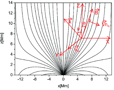
Figure 1: Funnel magnetic field geometry as obtained from the 2-D potential field model derived by Hackenberg et al. (2000). The field lines emerge from the boundary between two adjacent supergranules ($x=0$) and expand rapidly to fill the corona. The photospheric level is at $z=0$. Coordinate axes, wave vector and drift velocity are shown in red.

For the background plasma density and temperature we use the model of Fontenla et al. (1993) for the chromosphere and the model of Gabriel (1976) for the lower corona. The 2-D potential-field and current-free funnel model derived by Hackenberg et al. (2000) is used to define the background magnetic field (Fig.1). Analytically, this model is given by:

$$B_{0x}(x,z)=\frac{(B_{max}-B_{00})D}{2\pi(D-d)}ln\frac{cosh\frac{2\pi z}{D}-cos(\frac{\pi d}{D}+\frac{2\pi x}{D})}{cosh\frac{2\pi z}{D}-cos(\frac{\pi d}{D}-\frac{2\pi x}{D})}$$

$$B_{0z}(x,z)=B_{00}+(B_{max}-B_{00})\left[-\frac{d}{D-d}+\frac{D}{(D-d)\pi}\right.\times$$

$$\left(arctan\frac{cosh\frac{2\pi z}{D}\leavevmode\nobreak\ sin\frac{\pi d}{2D}+sin(\frac{\pi d}{2D}+\frac{2\pi x}{D})}{sinh\frac{2\pi z}{D}\leavevmode\nobreak\ cos\frac{\pi d}{2D}}+\right.$$

$$\left.\left.arctan\frac{cosh\frac{2\pi z}{D}\leavevmode\nobreak\ sin\frac{\pi d}{2D}+sin(\frac{\pi d}{2D}-\frac{2\pi x}{D})}{sinh\frac{2\pi z}{D}\leavevmode\nobreak\ cos\frac{\pi d}{2D}}\right)\right]$$

with the relevant parameters given as follow: D=30 Mm, d=0.34 Mm, $B_{00}$=11.8 G, $B_{max}$=1.5 kG.

To model nonuniformity, we consider the length scales of the background plasma density and pressure in the z-direction, H, to be much bigger than the one in the x-direction, L, i.e., $H=((1/n_{0j})\partial n_{0j}/{\partial z})^{-1}\gg L=((1/n_{0j})\partial n_{0j}/{\partial x})^{-1}$. Thus only a density gradient in the x-direction will be considered, for which use the following analytical density model:

$$n_{0j}(x)=n_{0j}(1+\frac{x}{L}),$$ (3)

whereby it is assumed that the density increases linearly in the x-direction, but only locally within the studied region where it is getting bigger by a factor 10. This assumption avoids a large growth of the density while the x-coordinate increases.

3 Linear perturbation analysis

The fluid equations associated with the particle species $j$ are given by:

$$\frac{\partial n_{j}}{\partial t}+\nabla\cdot(n_{j}\textbf{v}_{j})=0,$$ (4)

$$m_{j}n_{j}(\frac{\partial\textbf{v}_{j}}{\partial t}+\textbf{v}_{j}\cdot\nabla\textbf{v}_{j})+\nabla p_{j}-q_{j}n_{j}(\textbf{E}+\textbf{v}_{j}\times\textbf{B})=0,$$ (5)

$$\frac{\partial p_{j}}{\partial t}+\textbf{v}_{j}\cdot\nabla p_{j}+\gamma_{j}p_{j}\nabla\cdot\textbf{v}_{j}=0,$$ (6)

where $m_{j}$, $n_{j}$, $\textbf{v}_{j}$, $p_{j}$ and $\gamma_{j}$ are respectively the mass, density, velocity, pressure (which for simplicity is here assumed to be isotropic) and the polytropic index. The subscript $j$ stands for electron $e$, proton $p$ or alpha particle $\alpha$ (He²⁺). The electric field E and the magnetic field B are linked through Faraday’s law:

$$\nabla\times\textbf{E}=-\frac{\partial\textbf{B}}{\partial t}.$$ (7)

3.1 Linearization procedure

We express all the quantities in the above equations as a sum of an unperturbed stationary part (with subscript 0) and a perturbed part (with subscript 1) much smaller than the stationary part as follows:

$$n_{j}=n_{0j}(x)+n_{1j},\leavevmode\nobreak\ p_{j}=p_{0j}(x)+p_{1j},$$

$$\textbf{v}_{j}=\textbf{v}_{Dj}+\textbf{v}_{1j},\leavevmode\nobreak\ \textbf{B}=\textbf{B}_{0}(x,z)+\textbf{B}_{1},\leavevmode\nobreak\ \textbf{E}=\textbf{E}_{0}+\textbf{E}_{1},$$

$$n_{1j}\ll n_{0j},p_{1j}\ll p_{0j},\left|\textbf{v}_{1j}\right|\ll\left|\textbf{v}_{Dj}\right|,\left|\textbf{B}_{1}\right|\ll\left|\textbf{B}_{0}\right|,$$ (8)

where we have considered charge neutrality in the unperturbed stationary plasma, i.e., $\sum_{j}q_{j}n_{0j}=0$. Due to density stratification in the x-direction, a current is carried by drifting electrons and ions in opposite directions parallel to the y-axis, with a drift velocity given by:

$$\textbf{v}_{Dj}=-\frac{1}{L}\frac{C_{sj}^{2}}{\gamma_{j}\Omega_{j}}\frac{B_{0}}{B_{0z}}\textbf{\^{y}},$$ (9)

where $C_{sj}=\sqrt{\gamma_{j}k_{B}T_{j}/m_{j}}$ and $\Omega_{j}=q_{j}B_{0}/m_{j}$ are, respectively, the acoustic speed and the cyclotron frequency of the species $j$, and $k_{B}$ is the Boltzman constant.

The zero-order terms cancel out when Eq.(8) is inserted into the multi-fluid Eqs.(4)-(6). Neglecting the products of first-order nonlinear terms, we get a system of linear equations:

$$i(\omega-\textbf{k}\cdot\textbf{v}_{Dj})\frac{n_{1j}}{n_{0j}}-\textbf{v}_{1j}\cdot\frac{\nabla n_{0j}}{n_{0j}}-i\textbf{k}\cdot\textbf{v}_{1j}=0,$$ (10)

$$i(\omega-\textbf{k}\cdot\textbf{v}_{Dj})\textbf{v}_{1j} + \frac{\Omega_{j}}{\left|\textbf{B}_{0}\right|}\left(\textbf{E}_{1}+\textbf{v}_{1j}\times\textbf{B}_{0}+\textbf{v}_{Dj}\times\textbf{B}_{1}\right)$$ (11)

$$- C_{sj}^{2}\left(i\frac{p_{1j}}{p_{0j}}\textbf{k}-\frac{n_{1j}}{n_{0j}}\frac{\nabla p_{0j}}{p_{0j}}\right)=0,$$

$$i(\omega-\textbf{k}\cdot\textbf{v}_{Dj})\frac{p_{1j}}{p_{0j}}-\textbf{v}_{1j}\cdot\frac{\nabla p_{0j}}{p_{0j}}-i\gamma_{j}\textbf{k}\cdot\textbf{v}_{1j}=0,$$ (12)

where all the perturbed quantities have been expressed in terms of the amplitudes of plane waves. Fourier analysis has turned all derivatives into factors: $\partial/\partial t\rightarrow-i\omega$ and $\nabla\rightarrow i\textbf{k}$, where $\omega$ is the wave frequency and k the wave vector. Note that in Eq. (11) the term $\textbf{v}_{1j}\cdot\nabla\textbf{v}_{Dj}$ has been neglected in comparison with the term $(\textbf{k}\cdot\textbf{v}_{Dj})\textbf{v}_{1j}$ since it is smaller by the ratio $2\pi L_{B_{0z}}/\lambda$ where $L_{B_{0z}}=(|\nabla{B}_{0z}|/B_{0z})^{-1}$ is the length scale of the z-component of the background magnetic field and $\lambda$ the wave length of interest, i.e.:

$$\textbf{v}_{1j}\cdot\nabla\textbf{v}_{Dj}/(\textbf{k}\cdot\textbf{v}_{Dj})\textbf{v}_{1j} \approx L_{B_{0z}}^{-1}/(2\pi/\lambda)$$ (13)

$$\approx\lambda/(6L_{B_{0z}})\approx 10^{-5}\ll 1.$$

In this context we want to mention, and remind the reader of, the classical guiding-center drift caused by the gravity force (g is the gravitational acceleration) in a magnetic field, i.e.:

$$\textbf{v}_{gj}=\frac{1}{\Omega_{j}}\textbf{g}\times\frac{\textbf{B}}{\mid\textbf{B}\mid}.$$ (14)

In the corona this drift would lead to a current perpendicular to the magnetic field, and could thus also provide free energy which, as was shown in considerable detail by Brinca et al. (2002, 2003), could lead to various kinds of plasma instabilities and wave excitation. In comparison with Eq.(9), we obtain as an order-of-magnitude estimate for the ratio of these two drift speeds the result:

$$\frac{v_{gj}}{v_{Dj}}\approx\frac{g}{\Omega_{j}}\frac{\Omega_{j}L}{C_{sj}^{2}}\approx\frac{L}{H},$$ (15)

where we used again the gravitational scale height $H$ as defined in the previous section for the background density being thermally stratified in the z-direction. So the small horizontal density variation considered here yields a larger drift than the one induced by vertical gravity. However, transverse currents driven by gravitational stratification may play a role in generating plasma instability at the gyrokinetic scale, but the growth rate is expected to be smaller by the ratio $H/L$.

3.2 Dispersion relation

The above linearized equations are combined in order to obtain a linear relation between the current density $\textbf{J}_{1}$ and the electric field $\textbf{E}_{1}$:

$$\textbf{J}_{1}=\@vec{\sigma}\cdot\textbf{E}_{1},$$ (16)

where $\@vec{\sigma}$ is the conductivity tensor which is related to the dielectric tensor $\@vec{\epsilon}$ through the following relation:

$$\@vec{\epsilon}=\textbf{I}+\frac{i}{\omega\varepsilon_{0}}\@vec{\sigma}.$$ (17)

The dispersion relation is obtained using electrodynamics theory (e.g., Stix 1992):

$$D(\omega,\textbf{k},\textbf{r})=\textrm{Det}\left[\frac{c^{2}}{\omega^{2}}\textbf{k}\times(\textbf{k}\times\textbf{E})+\@vec{\epsilon}(\omega,\textbf{k},\textbf{r})\cdot\textbf{E}\right]=0,$$ (18)

where $c$ is the speed of light in vacuum and r is the large-scale position vector.

3.3 Ray-tracing equations

Considering the WKB approximation, the ray-tracing problem consists in solving a system of ordinary differential equations of the Hamiltonian form (Weinberg 1962; Lighthill 1978). These equations, that solve for the wave frequency $\omega$, the wave vector k and the space coordinate r, have been formulated by Bernstein & Friedland (1984), and in the simple case of a Hermitian dielectric tensor are given by:

$$\frac{\textrm{d}\omega}{\textrm{d}t}=-\frac{\partial D(\omega,\textbf{k},\textbf{r})/\partial t}{\partial D(\omega,\textbf{k},\textbf{r})/\partial\omega}=0,$$ (19)

$$\frac{\textrm{d}\textbf{k}}{\textrm{d}t}=\leavevmode\nobreak\ \frac{\partial D(\omega,\textbf{k},\textbf{r})/\partial\textbf{r}}{\partial D(\omega,\textbf{k},\textbf{r})/\partial\omega},$$ (20)

$$\frac{\textrm{d}\textbf{r}}{\textrm{d}t}=-\frac{\partial D(\omega,\textbf{k},\textbf{r})/\partial\textbf{k}}{\partial D(\omega,\textbf{k},\textbf{r})/\partial\omega}\cdot$$ (21)

A generalization of these equations to the case of an anti-Hermitian dielectric tensor was also proposed by Bernstein & Friedland (1984). In this case, additionally to the ray path, the growth rate of the instability can also be computed. Note that Eq.(19) is set to zero since the dispersion relation does not depend explicitly on the time $t$ (the background plasma is stationary). The above differential equations represent a set of initial values problem which can be solved using initial conditions obtained from the local solutions of the dispersion relation (Eq.18).

4 Numerical results

4.1 Local stability analysis

The dispersion relation Eq.(18) is solved numerically for the funnel location (x=9.4 Mm, z=2.5 Mm) characterized by a magnetic field inclination angle of $\varphi=85.3^{\circ}$ with respect to the normal on the solar surface. The value of the density length scale in the x-direction, L, is chosen to be 1 km according to results obtained from radio propagation measurements (Woo 1996, 2006). We consider the cases of a two-fluid (e-p) and a three-fluid (e-p-He²⁺) model, where we consider the effect a second ion population of alpha particles (He²⁺) with typical coronal abundance. First, the local solutions of the dispersion relation Eq.(18) are presented, and then the results obtained from the non-local ray-tracing equations.

4.1.1 Two-fluid (e-p) drift-plasma

x=9.4 Mm, z=2.5 Mm,  $\varphi\approx 85.3^{\circ}$, $\theta=85^{\circ}$

Figure 2: Two-fluid dispersion curves at the funnel location (x=9.4 Mm, z=2.5 Mm) with a B₀-inclination angle $\varphi=85.3^{\circ}$. The angle of propagation is $\theta=85^{\circ}$. Top: The case of a uniform plasma density, i.e. $v_{Dj}=0$, with a plasma beta $\beta_{e}=\beta_{p}\approx 0.0097$. Bottom: In the presence of a drift due to a density gradient with a scale length of L=1 km. Here $\omega$ and $k$ are normalized, respectively, to the proton cyclotron frequency, $\Omega_{p}$, and the proton inertial length, $\Omega_{p}/V_{Ap}$, where $V_{Ap}=B_{0}/\sqrt{\mu_{0}n_{0p}m_{p}}$ is the proton Alfvén speed ($\mu_{0}$ is the magnetic permeability in vacuum). Here $T_{0e}=T_{0p}$.

The two-fluid drift-plasma configuration consists of a plasma made of electrons with density $n_{0e}$ and protons ($n_{0p}$) in relative drift to each other in opposite directions along the y-axis and perpendicular to the background magnetic field with velocities given by Eq.(9). The drift velocity is sustained by the presence of a local density gradient in the x-direction, as described by Eq.(3). For the purpose of comparison, the dispersion curves in the case of a vanishing density gradient, L^-1=0, and thus no relative drift between electrons and ions, i.e., $v_{De}$=$v_{Dp}$=0, are given in the top panel of Fig.2, corresponding to an angle of propagation $\theta=85^{\circ}$. Consequently, there is no free energy in the plasma, and all the modes remain stable. In this case the dispersion relation Eq.(18) is quadratic and three stable modes are present. Each one is represented by an oppositely propagating ($\omega>0$ and $\omega<0$) pair of waves. These modes represent the extensions of the usual Slow (dotted line), Alfvén (dashed line), and Fast (solid line) MHD modes into the high-frequency domain around $\omega=\Omega_{p}$ (=$eB_{0}/m_{p}$), where these waves become dispersive.

However, in the case L=1 km, the relative drift between electrons and protons is not zero, and the dispersion curves are strongly modified with a breaking of the symmetry between forward ($\omega>0$) and backward ($\omega<0$) propagating waves, as it is shown in the bottom panel of Fig.2. This behavior affects particularly the slow mode. Indeed, the free energy provided by the relative drift between electrons and protons, which is sustained by the density gradient, leads to the appearance of regions of instability resulting from the coupling between forward and backward propagating slow modes. These two single initially stable modes couple into one single unstable mode, for which the normalized growth rate $\gamma/\Omega_{p}$ is given by the red curve, which does not exceed 0.007.

As it is shown in the top panel of Fig.3, for small angle of propagation, this instability is very weak and concentrated at small wave number $kV_{Ap}/\Omega_{p}\ll 1$, and extends to larger k with sensitively bigger growth rate $\gamma$ at large angle of propagation $\theta$. This instability is also shown in the bottom panel of Fig.3 as a function of the propagation angle $\theta$ and the length scale of the density gradient L in the x-direction at the location (x=9.4 Mm, z=2.5 Mm). It is clearly seen, that with increasing L, the instability growth rate decreases and covers gradually a smaller range in the angle of propagation $\theta$. The maximum growth rate is $\gamma/\Omega_{p}\approx 0.008$ for L=1 km and for $\theta$ between 75^∘ and 85^∘. For larger L, the growth rate decreases and the instability appears only at large angles of propagation ($\theta\gtrsim 85^{\circ}$). This result is expected since the larger the length scale of density L is the more decreases the particles drift speed, by virtue of (Eq.9), providing thus less free energy to the plasma for driving the instability.

x=9.4 Mm, z=2.5 Mm,  $\varphi\approx 85.3^{\circ}$

Figure 3: Growth rate of the two-fluid instability resulting form the coupling between forward and backward propagating slow modes at the funnel location (x=9.4 Mm, z=2.5 Mm) with a B₀-inclination angle of $\varphi=85.3^{\circ}$. Top: As a function of the angle of propagation $\theta$ and the normalized wave number, $kV_{Ap}$/$\Omega_{p}$, for a density length-scale in the x-direction of L=1 km ($v_{Dp}=v_{De}\approx 0.0057V_{Ap}$). Bottom: As a function of $\theta$ and L for $kV_{Ap}/\Omega_{p}=1$.

4.1.2 Three-fluid (e-p-He²⁺) drift-plasma

x=9.4 Mm, z=2.5 Mm,  $\varphi\approx 85.3^{\circ}$, $\theta=85^{\circ}$

Figure 4: Three-fluid dispersion curves at the location (x=9.4 Mm, z=2.5 Mm) with a B₀-inclination angle $\varphi=85.3^{\circ}$. The angle of propagation is $\theta=85^{\circ}$. Top: The case of a uniform plasma, i.e., $v_{Dj}=0$, with the plasma-beta $\beta_{e}=1.2\beta_{p}=4\beta_{\alpha}\approx 0.0097$. Bottom: In the presence of a drift due to a density gradient with a length scale L=1 km. Here $T_{0\alpha}=3T_{0p}=3T_{0e}$.

In the three-fluid drift-plasma configuration, in addition to electrons ($n_{0e}$) and protons ($n_{0p}$), we consider the presence of a second population of ions, namely alpha particles He²⁺ (indicated by $\alpha$) with a typical coronal abundance of $n_{0\alpha}=0.1n_{0p}$. The electrons and ions are in opposite relative drift according to Eq.(9) and caused by the presence of a density gradient in the x-direction as in Eq.(3).

For the purpose of comparison, the dispersion curves in the case of L^-1=0 (zero gradient of density) and consequently $v_{De}$=$v_{Dp}$=$v_{D\alpha}$=0, are again given in the top panel of Fig.4, corresponding to the location (x=9.4 Mm, z=2.5 Mm) with $\varphi=85.3^{\circ}$ and to an angle of propagation $\theta=85^{\circ}$. In this case the dispersion relation Eq.(18) is quadratic and the dispersion diagrams show the presence of five stable modes. Each one of them is represented by an oppositely propagating ($\omega>0$ and $\omega<0$) pair of waves. We note the presence of: slow modes 1 and 2 (respectively dotted and dashed-dot-dot lines), intermediate modes 1 and 2 (dashed and dashed-dot lines), and one fast mode which is not shown here because it presents a cut-off frequency around $\omega_{co}\approx 0.6\Omega_{p}$, which is out of the frequency range presented in this study (for further details see Mecheri & Marsch 2006). Consequently, the consideration of a second population of ions leads to the appearance of an additional slow and ion-cyclotron mode.

x=9.4 Mm, z=2.5 Mm,  $\varphi\approx 85.3^{\circ}$

Figure 5: Growth rate of the three-fluid slow mode 2 instability which is resulting from the coupling between forward and backward propagating slow modes and is absent in the two-fluid case. The results are given for the funnel location (x=9.4 Mm, z=2.5 Mm) with a B₀-inclination angle of $\varphi=85.3^{\circ}$. Top: As a function of the angle of propagation $\theta$ and the normalized wave number $kV_{Ap}$/$\Omega_{p}$ for a density-length scale in the x-direction of L=1 km ($v_{De}=1.2v_{Dp}=4v_{D\alpha}\approx 0.0057V_{Ap}$). Bottom: As a function of $\theta$ and L for $kV_{Ap}/\Omega_{p}=1$.

In the case a non-zero density gradient in the $x$-direction characterized by a length scale L=1 km, the dispersion relation is not quadratic anymore, and the symmetry between forward and backward propagating modes is broken (bottom panel of Fig.4). Indeed, the free energy provided by the relative drift between electrons and ions sustained by the density gradient leads to the appearance of regions of instability. The first instability is similar to the one found in the two-fluid model It results from the coupling between forward and backward propagating slow modes 1. The second instability results from the coupling between forward and backward propagating slow modes 2 with a sensitively smaller growth rate, $\gamma\lesssim 0.0015\Omega_{p}$ as compared to the first one. This instability appears in general at very large angle of propagation, i.e. $\theta\gtrsim 84^{\circ}$ (top panel of Fig.5). As $\theta$ increases, the growth rate appears in two different ranges of the wavenumber k, the first at small k, i.e. $kV_{Ap}/\Omega_{p}\lesssim 3$, and the second at larger k, i.e. $kV_{Ap}/\Omega_{p}\gtrsim 5$. The instability growth rate in general increases sensitively between $kV_{Ap}/\Omega_{p}\approx 4$ and 8, and has its maximum for $kV_{Ap}/\Omega_{p}\approx 5$. However, it is approximately 6 times smaller than the slow-mode-1 maximum instability growth rate. When plotted as a function of the propagation angle $\theta$ and the length scale of the density gradient L (bottom panel of Fig.5), this instability mainly appears at large angle of propagation, i.e. $\theta\gtrsim 87^{\circ}$, and the corresponding growth rate decreases with increasing L. The maximum growth rate occurs for L=1 km and for a propagation angle around 88^∘.

4.2 Non-local stability analysis

In this section we perform a non-local wave study using the ray-tracing equations presented in Sect.(3.3). These equations are computed using initial conditions obtained from the local solutions of the dispersion relation Eq.(18) at the starting location (x₀=9.4 Mm, y₀=0 Mm, z₀=2.5 Mm). We consider both the two-fluid (e-p) and the three-fluid (e-p-He²⁺) case with a constant concentration of the alpha particles (He²⁺), i.e. $n_{\alpha}=0.1n_{p}$ along the ray path. The density length scale in the x-direction L is chosen to be 1 km.

Two-fluid (e-p) drift-plasma

As presented in the previous section, in the two-fluid case the local solution of the dispersion relation showed the presence of an instability resulting from the coupling between forward and backward propagating slow modes. The ray path of this unstable wave, as well as the spatial variation of its growth rate $\gamma$, when the wave is launched at the initial location (x₀=9.4 Mm, y₀=0, z₀=2.5 Mm), are presented on Fig.6. The results are shown for different initial angle of propagation $\theta_{0}$, with which a different initial normalized wave number $k_{0}$ is associated that is chosen to always correspond to the maximum growth rate $\gamma_{max}$. The wave starts propagating from its initial location and is well guided along the field lines up to approximately the location x$\approx$11 Mm and z$\approx$2.6 Mm, where its motion starts to become unguided and irregular (see Fig.6a, 6b and 6c). This unguided motion continues until the wave reaches a maximum height where it is reflected and starts to propagate downward almost in the (y,z) plane to reach again its initial height, i.e., z=2.5 Mm. This maximum height reached by the unstable wave is larger for smaller initial angle of propagation $\theta_{0}$. Additionally, the smaller $\theta_{0}$ is the more deeply can the wave propagate in the y-direction. The corresponding instability growth rate $\gamma$ is very irregular, and increases and decreases intermittently along the ray path (Fig.6d and 6e). The growth rate $\gamma$ shows the appearance of peaks of maximum instability, which are more important for large initial propagation angle $\theta_{0}$ but do not exceed $\gamma=0.025\Omega_{p}$. However, the instability growth ceases at approximately the maximum height reached by the wave, from where on it starts propagating downward.

x₀=9.4 Mm, y₀=0, z₀=2.5 Mm,  $\varphi\approx 85.3^{\circ}$

Figure 6: Ray trajectory and growth rate of the two-fluid slow modes instability. The waves are launched at the initial location (x₀=9.4 Mm, y₀=0, z₀=2.5 Mm) in the coronal funnel (with a B₀-inclination angle of $\varphi_{0}\approx 85.3^{\circ}$) and for different initial angle of propagation $\theta_{0}$ and normalized wave number $k_{0}$, chosen for each $\theta_{0}$ at the maximum growth rate. The dashed lines represent the funnel magnetic field lines. (a) 3-D ray path; (b) Projection of the ray path on the x-z plane; (c) Ray path projected on the y-z plane; (d) Growth rate as a function of the z-coordinate; (e) Growth rate as a function of the y-coordinate.

Three-fluid (e-p-He²⁺) drift-plasma configuration

x₀=9.4 Mm, y₀=0, z₀=2.5 Mm,  $\varphi\approx 85.3^{\circ}$

Figure 7: Ray trajectory and growth rate of the three-fluid slow mode 2 instability which is absent from the two-fluid model. The waves are launched at the initial location (x₀=9.4 Mm, y₀=0, z₀=2.5 Mm) in the coronal funnel (with a B₀-inclination angle of $\varphi_{0}\approx 85.3^{\circ}$) and for different initial angle of propagation $\theta_{0}$ and normalized wave number $k_{0}$, chosen for each $\theta_{0}$ at the maximum growth rate. The dashed lines represent the funnel magnetic field lines. (a) 3-D ray path; (b) Projection of the ray path on the x-z plane; (c) Ray path projected on the y-z plane; (d) Growth rate as a function of the z-coordinate; (e) Growth rate as a function of the y-coordinate.

In this three-fluid model case, and at the location (x=9.4 Mm, z=2.5 Mm), the solution of the dispersion relation shows the presence of two instabilities both resulting from the coupling between forward and backward propagating slow modes. For the first instability, which is similar to the one obtained in the case of the two-fluid model, the ray path as well as the spatial variation of its growth rate $\gamma$ show a similar behavior as in the two-fluid case. The ray path as well as the growth rate variation of the second instability, when the wave is launched at the initial location (x₀=9.4 Mm, y₀=0, z₀=2.5 Mm), are presented in Fig.7. The results show that the unstable wave starts to propagate as a guided mode for a very small distance but then is rapidly reflected to propagate downward (Fig.7a, 7b and 7c). Additionally, the waves propagates only to a very short distance in the y-direction, i.e. $y<0.004$ Mm (Fig.7c).

5 Conclusion

We have studied gradient-drift electromagnetic instabilities in a coronal funnel, using a collisionless two-fluid (e-p) and three-fluid (e-p-He²⁺) plasma model with finite pressure. While neglecting electron inertia, this model allows us to take ion-cyclotron wave effects into account. We have considered a density stratification transverse to the ambient magnetic field with the typical small length scales suggested by the observations.

First, a local perturbation analysis has been performed, whereby the dispersion relation has been solved for a local region in a coronal funnel. By comparison with the results obtained for a uniform-density plasma, it was found that the dispersion curves are strongly modified. For certain ranges of the wave number, two initially stable modes merge into a single unstable mode. Indeed, the free energy provided by the relative drift between the different plasma species due to the density gradient leads to the appearance of regions of instability. In the two-fluid model, this instability results from the coupling between forward and backward propagating slow modes. For large angles of propagation this instability extends over a wide range in wave number and is characterized by a small phase speed and an increasing growth rate as the angle of propagation (with respect to the normal on the solar surface) increases.

In addition, the consideration of a second ion population of alpha particles (He²⁺) with typical coronal abundance led to the appearance of a new instability which also results from the coupling of oppositely propagating slow mode waves. However, this second instability in general covers only a small range in the wavenumber domain and exists mainly for very large angles of propagation $\gtrsim 82^{\circ}$, and it has a substantially smaller growth rate by approximately a factor 6 as compared to the first instability.

The non-local analysis, which has been performed using ray-tracing equations, revealed that the unstable waves, from their launching point, start to propagate upward for a very small distance but then are reflected and propagate downward. During this propagation, the corresponding instability growth rate has a variable character and is increasing, decreasing and vanishing intermittently.

Consequently, drift currents caused by the fine structuring of the density in the magnetically open funnels of a coronal hole can provide enough energy for driving plasma micro-instabilities. They may in turn constitute a prolific source of the high-frequency ion-cyclotron waves that have been invoked to play, through kinetic wave dissipation, a prominent role in heating the open corona.

References

- Aschwanden et al. (2000) Aschwanden, M. J., Nightingale, R. W., & Alexander, D. 2000, ApJ, 541, 1059
- Axford & McKenzie (1992) Axford, W. I. & McKenzie, J. F. 1992, in Solar Wind Seven Colloquium, ed. E. Marsch & R. Schwenn, 1–5
- Axford & McKenzie (1995) Axford, W. I. & McKenzie, J. F. 1995, in Solar Wind Conference, 31
- Bernstein & Friedland (1984) Bernstein, I. B. & Friedland, L. 1984, in Basic Plasma Physics: Selected Chapters, Handbook of Plasma Physics, Volume 1, ed. A. A. Galeev & R. N. Sudan, 367–+
- Brinca et al. (2002) Brinca, A. L., Romeiras, F. J., & Gomberoff, L. 2002, Journal of Geophysical Research (Space Physics), 107, 1090
- Brinca et al. (2003) Brinca, A. L., Romeiras, F. J., & Gomberoff, L. 2003, Journal of Geophysical Research (Space Physics), 108, 1038
- Cranmer et al. (1999) Cranmer, S. R., Field, G. B., & Kohl, J. L. 1999, ApJ, 518, 937
- Cranmer & van Ballegooijen (2005) Cranmer, S. R. & van Ballegooijen, A. A. 2005, ApJS, 156, 265
- Fontenla et al. (1993) Fontenla, J. M., Avrett, E. H., & Loeser, R. 1993, ApJ, 406, 319
- Gabriel (1976) Gabriel, A. H. 1976, Royal Society of London Philosophical Transactions Series A, 281, 339
- Hackenberg et al. (2000) Hackenberg, P., Marsch, E., & Mann, G. 2000, A&A, 360, 1139
- Heyvaerts & Priest (1983) Heyvaerts, J. & Priest, E. R. 1983, A&A, 117, 220
- Hollweg (1986) Hollweg, J. V. 1986, J. Geophys. Res., 91, 4111
- Hu et al. (1999) Hu, Y. Q., Habbal, S. R., & Li, X. 1999, J. Geophys. Res., 104, 24819
- Ionson (1982) Ionson, J. A. 1982, ApJ, 254, 318
- Isenberg (1990) Isenberg, P. A. 1990, J. Geophys. Res., 95, 6437
- Kohl et al. (1997) Kohl, J. L., Noci, G., Antonucci, E., et al. 1997, Sol. Phys., 175, 613
- Li et al. (1999) Li, X., Habbal, S. R., Hollweg, J. V., & Esser, R. 1999, J. Geophys. Res., 104, 2521
- Lighthill (1978) Lighthill, J. 1978, Waves in fluids (Cambridge, Cambridge University Press, 1978. 516 p.)
- Markovskii (2001) Markovskii, S. A. 2001, ApJ, 557, 337
- Markovskii & Hollweg (2002) Markovskii, S. A. & Hollweg, J. V. 2002, Journal of Geophysical Research (Space Physics), 107, 21
- Markovskii & Hollweg (2004a) Markovskii, S. A. & Hollweg, J. V. 2004a, ApJ, 609, 1112
- Markovskii & Hollweg (2004b) Markovskii, S. A. & Hollweg, J. V. 2004b, Nonlinear Processes in Geophysics, 11, 485
- Markovskii et al. (2006) Markovskii, S. A., Vasquez, B. J., Smith, C. W., & Hollweg, J. V. 2006, ApJ, 639, 1177
- Marsch & Tu (1990a) Marsch, E. & Tu, C.-Y. 1990a, J. Geophys. Res., 95, 8211
- Marsch & Tu (1990b) Marsch, E. & Tu, C.-Y. 1990b, J. Geophys. Res., 95, 11945
- Marsch & Tu (2001) Marsch, E. & Tu, C.-Y. 2001, J. Geophys. Res., 106, 227
- Matthaeus et al. (1999) Matthaeus, W. H., Zank, G. P., Oughton, S., Mullan, D. J., & Dmitruk, P. 1999, ApJL, 523, L93
- McEwan & de Moortel (2006) McEwan, M. P. & de Moortel, I. 2006, A&A, 448, 763
- Mecheri & Marsch (2006) Mecheri, R. & Marsch, E. 2006, Royal Society of London Philosophical Transactions Series A, 364, 537
- Mecheri & Marsch (2007) Mecheri, R. & Marsch, E. 2007, A&A, 474, 609
- Ofman et al. (2002) Ofman, L., Gary, S. P., & Viñas, A. 2002, Journal of Geophysical Research (Space Physics), 107, 9
- Stix (1992) Stix, T. H. 1992, Waves in Plasmas (Waves in Plasmas, New York: American Institute of Physics, 1992)
- Tu (1988) Tu, C.-Y. 1988, J. Geophys. Res., 93, 7
- Voitenko & Goossens (2002) Voitenko, Y. & Goossens, M. 2002, Sol. Phys., 206, 285
- Weinberg (1962) Weinberg, S. 1962, Physical Review, 126, 1899
- Woo (1996) Woo, R. 1996, Nature, 379, 321
- Woo (2006) Woo, R. 2006, ApJ, 639, L95
- Zhang (2003) Zhang, T. X. 2003, ApJ, 597, L69