Spectroscopy of clusters in the ESO distant cluster survey (EDisCS).II.

Abstract

Aims. We present spectroscopic observations of galaxies in 15 survey fields as part of the ESO Distant Cluster Survey (EDisCS). We determine the redshifts and velocity dispersions of the galaxy clusters located in these fields, and we test for possible substructure in the clusters.

Methods. We obtained multi-object mask spectroscopy using the FORS2 instrument at the VLT. We reduced the data with particular attention to the sky subtraction. We implemented the method of Kelson for performing sky subtraction prior to any rebinning/interpolation of the data. From the measured galaxy redshifts, we determine cluster velocity dispersions using the biweight estimator and test for possible substructure in the clusters using the Dressler–Shectman test.

Results. The method of subtracting the sky prior to any rebinning/interpolation of the data delivers photon-noise-limited results, whereas the traditional method of subtracting the sky after the data have been rebinned/interpolated results in substantially larger noise for spectra from tilted slits. Redshifts for individual galaxies are presented and redshifts and velocity dispersions are presented for 21 galaxy clusters. For the 9 clusters with at least 20 spectroscopically confirmed members, we present the statistical significance of the presence of substructure obtained from the Dressler–Shectman test, and substructure is detected in two of the clusters.

Conclusions. Together with data from our previous paper, spectroscopy and spectroscopic velocity dispersions are now available for 26 EDisCS clusters with redshifts in the range 0.40–0.96 and velocity dispersions in the range $166\,\mathrm{km}\,\mathrm{s}^{-1}$–$1080\,\mathrm{km}\,\mathrm{s}^{-1}$.

1 Introduction

Galaxy clusters provide important environments for the study of galaxy evolution out to high redshift (e.g. Aragón-Salamanca et al. 1993). They are detectable at optical wavelengths (e.g. Abell 1958; Zwicky et al. 1968; Shectman 1985; Gunn et al. 1986; Couch et al. 1991; Postman et al. 1996; Gladders & Yee 2000; Gonzalez et al. 2001; Wilson et al. 2006; Scoville et al. 2007), by the X-ray (e.g. Rosati et al. 1995; Finoguenov et al. 2007 and references therein) and radio (Feretti & Giovannini 2007) emission of their intracluster medium (ICM) and point sources, and by the scattering of cosmic background radiation by ICM free electrons via the Sunyaev-Zel’dovich effect (e.g. Sunyaev & Zeldovich 1970; Carlstrom et al. 2002; Birkinshaw & Lancaster 2007).

Spectroscopic surveys of cluster galaxies began with work on Coma and Perseus by Kent & Gunn (1982) and Kent & Sargent (1983), and progressed to the systematic studies of tens of local clusters by Dressler & Shectman (1988) and Zabludoff et al. (1990). Currently, the most comprehensive spectroscopic catalogues of local galaxy clusters are provided by applying a variety of selection techniques to large-area surveys, primarily the Sloan Digital Sky Survey (SDSS) from which the C4 Miller et al. (2005) and MaxBCG Koester et al. (2007) catalogues are produced.

Intermediate redshift ($z\sim 0.2$–$0.7$) spectroscopic cluster surveys arrived with the work of the CNOC (Yee et al. 1996; Balogh et al. 1997) and MORPHS (Dressler et al. 1999; Poggianti et al. 1999) collaborations. Further kinematic studies of individual and small samples of intermediate redshift clusters include those by Kelson et al. (1997, 2006), Tran et al. (2003), Bamford et al. (2005), Serote Roos et al. (2005) and Moran et al. (2005).

At higher redshift ($z\sim 0.7$–$1.3$) surveys have been completed by Postman et al. (1998, 2001), and a number of individual clusters have been studied (e.g. van Dokkum et al. 2000; Jørgensen et al. 2005, 2006; Tanaka et al. 2006; Demarco et al. 2007; Tran et al. 2007). However, to date our knowledge of clusters beyond $z\sim 0.5$ has been generally limited to the highest-mass systems.

Cluster velocity dispersions provide a measure of cluster mass (Fisher et al. 1998; Tran et al. 1999; Borgani et al. 1999; Lubin et al. 2002). The measurement of cluster velocity dispersions should be made using statistics insensitive to galaxy redshift outliers and the shape of the velocity distribution, e.g. the biweight scale and gapper estimators proposed by Beers et al. (1990) (e.g. Halliday et al. 2004). Galaxy clusters may however have cluster substructure (Dressler & Shectman 1988; Geller & Beers 1982). Substructure can take many forms (e.g., bimodality, small clumps, filaments) and its detection constitutes a non–trivial technical problem. Many statistical tests have been developed and applied to reasonably large samples of clusters over the past decades. They all agree with the conclusion that substructure is an important phenomenon, but often diverge quite significantly on the fraction of clusters exhibiting significant substructure. As an example, Dressler & Shectman (1988) adopted a method to quantify the significance of cluster substructure using galaxy spectroscopic redshifts and projected sky positions. The presence of substructure suggests that the galaxy cluster is still relaxing. This may imply that the cluster velocity dispersion is a less reliable measure of cluster mass, although our limited data for 3 clusters with detected substructure and with a measured lensing mass do not indicate this (Fig. 18).

In this paper we present cluster velocity dispersion measurements and assessment of cluster substructure for 21 galaxy clusters from the ESO Distant Cluster Survey (EDisCS) located in 15 survey fields. Measurements for the 5 remaining clusters located in 5 survey fields were presented in Halliday et al. (2004).

EDisCS (White et al. 2005) is a project to study high-redshift cluster galaxies, as well as coeval field galaxies, in terms of their sizes, luminosities, morphologies, internal kinematics, star formation properties and stellar populations. We achieve this by obtaining deep multi-band imaging of 20 survey fields containing clusters at $z$ = 0.4–1 and deep spectroscopy of $\sim$100 galaxies per field. The EDisCS fields were chosen to target galaxy cluster candidates from the Las Campanas Distant Cluster Survey (LCDCS, Gonzalez et al. 2001). The LCDCS is a survey of an area of 130 square degrees imaged in a single wide optical filter using a 1 m telescope in drift-scan mode with an effective exposure time of 3.2 minutes. All detected objects are removed. For a high-redshift cluster this only affects a few of the brightest galaxies in the cluster; the rest of the galaxies are not detected individually. High-redshift clusters can then be detected as diffuse light peaks with a typical scale of 10^′′, resulting in a catalogue of 1073 cluster candidates with estimated redshifts $z_{\mathrm{est}}$ = 0.3–1.0. From this catalogue we selected 30 of the highest surface-brightness candidate clusters. Using moderately deep 2–band VLT/FORS2 imaging (going 3 magnitudes deeper than the original LCDCS imaging), 28 of the candidates were found to show a significant overdensity of red galaxies close to the LCDCS position (Gonzalez et al. 2002). From these clusters, we selected 10 clusters at $z_{\mathrm{est}}\approx 0.5$ (hereafter mid–$z$) and 10 clusters at $z_{\mathrm{est}}\approx 0.8$ (hereafter high–$z$) to constitute the EDisCS sample. These fields were imaged optically in $BVI$ (mid–$z$) and $VRI$ (high–$z$) with VLT/FORS2 using 14 nights (White et al. 2005), and in the near-infrared (NIR) in $K$ (mid–$z$) and $JK$ (high–$z$) with NTT/SOFI using 20 nights (Aragón-Salamanca et al., in prep.). Spectroscopy was obtained using VLT/FORS2 using 22 nights (Halliday et al. 2004 and this paper). Follow-up observations include MPG/ESO 2.2m/WFI wide field imaging in $VRI$ of all fields, HST/ACS imaging in F814W of 10 fields (Desai et al. 2007), H$\alpha$ narrow-band imaging (Finn et al. 2005), XMM–Newton/EPIC X–ray observations (Johnson et al. 2006), and Spitzer IRAC (3–8$\mu$m) and MIPS (24$\mu$m) imaging. The legacy value of the EDisCS fields has been further increased by another ESO Large Programme that studies galaxies at redshift 5–6 in 10 of the EDisCS fields, using the EDisCS imaging as well as new deep VLT/FORS2 $z$–band imaging and spectroscopy (cf. Douglas et al. 2007).

The unprecedented novelty of the EDisCS dataset stems from the range of cluster velocity dispersions and masses covered by the sample. On the one hand, the survey provides high-redshift counterparts to the lower velocity dispersion clusters abundant in the local universe. On the other hand, it probes a range in cluster masses large enough to allow the study of the dependency on cluster mass of the processes affecting cluster galaxy evolution. The scientific exploitation of the rich EDisCS dataset is ongoing, but it has already produced important results in this respect. Studies have so far been completed on the red-sequence galaxies (De Lucia et al. 2004, 2007), the star-forming galaxies as seen in H$\alpha$ (Finn et al. 2005) and [OII] (Poggianti et al. 2006), the cluster velocity dispersions (Halliday et al. 2004 and this paper), the weak-lensing mass reconstruction of the clusters (Clowe et al. 2006), the X–ray properties of the clusters (Johnson et al. 2006), the HST–based visual galaxy morphologies (Desai et al. 2007), the evolution of the early-type galaxy fraction (Simard et al. 2007), and the evolution of the brightest cluster galaxies (Whiley et al. 2007). Further studies of the properties of the cluster galaxies and the clusters themselves will follow.

This paper is organised as follows. Section 2 reports the target selection and the observations. Section 3 describes the data reduction using two different methods for the sky subtraction: sky subtraction performed after (respectively before) any rebinning/interpolation of the data has been done (cf. Kelson 2003). Section 4 presents the redshift measurements and the redshift histograms. Section 5 examines the success rate, the failure rate and potential selection biases. Section 6 describes the determination of cluster redshifts and velocity dispersions. Section 7 discusses possible cluster substructure. Section 8 discusses the velocity dispersions for the full sample of EDisCS clusters in comparison with the weak-lensing measurements and with other samples. Section 9 provides a summary, and Appendix A compares results from the two sky subtraction methods.

The discussed photometry is based on Vega zero-points unless stated otherwise. We assume a cosmology with $\Omega_{\mathrm{m}}=0.3$, $\Omega_{\Lambda}=0.7$ and $H_{0}=70\,\mathrm{km}\,\mathrm{s}^{-1}\,\mathrm{Mpc}^{-1}$.

2 Target selection and observations

The target selection strategy, mask design procedure and observations for the EDisCS spectroscopy are described in detail in Halliday et al. (2004). Here we give the main points. We also provide a table with the target selection parameters (Table 1), and we discuss the performance of the uphotometric redshifts used.

2.1 Target selection strategy

Table 1: Target selection parameters for the masks with long exposures in the 20 EDisCS fields

Field	$z_{\mathrm{cl}}^{\mathrm{final}}$	Run	Mask numbers	$z_{\mathrm{phot,low}}$	$z_{\mathrm{phot,high}}$	Explanation	$z_{\mathrm{cl}}^{\mathrm{P}}$	$I_{1,\mathrm{bright}}$	$I_{1,\mathrm{faint}}$	Filters
Mid–$z$ fields:
1018.8$-$1211	0.4734	3	05,06,07	0.27	0.67	$0.47\pm 0.2$	0.472	19.5	22	BVIK
1059.2$-$1253	0.4564	3	05,06,07	0.26	0.66	$0.46\pm 0.2$	0.457	19.6	22	BVIK
1119.3$-$1129	0.5500	4	09,10,11	0.35	0.75	$0.55\pm 0.2$	0.549	19.9	22	BVI
1202.7$-$1224	0.4240	4	09,10,11	0.22	0.62	$0.42\pm 0.2$	0.424	19.5	22	BVIK
		2	02,03,04	0.28	0.68	$0.48\pm 0.2$	0.54	18.6	22	BVI[J]K
1232.5$-$1250	0.5414	3	05	0.34	0.74	$0.54\pm 0.2$	0.541	19.7	22	BVI[J]K
1238.5$-$1144	0.4602	4	09	0.26	0.66	$0.46\pm 0.2$	0.465	19.2	22	BVI
1301.7$-$1139	0.4828, 0.3969	4	09,10,11	0.20	0.68	$0.40-0.2,0.48+0.2$	0.485	19.2	22	BVIK
1353.0$-$1137	0.5882	4	09,10,11	0.39	0.79	$0.59\pm 0.2$	0.577	19.6	22	BVIK
1411.1$-$1148	0.5195	3	05,06,07	0.32	0.72	$0.52\pm 0.2$	0.520	19.4	22	BVIK
1420.3$-$1236	0.4962	4	09,10,11	0.30	0.70	$0.50\pm 0.2$	0.497	19.5	22	BVIK
High–$z$ fields:
1037.9$-$1243	0.5783, 0.4252	3	05,06,07,08	0.38	0.78	$0.58\pm 0.2$	0.58	20.0	23	VRIJK
		2	02,03,04	0.5031	0.9031	$0.70\pm 0.2$	0.55	19.5	23	VRIJK
1040.7$-$1155	0.7043	3	05,06	0.504	0.904	$0.70\pm 0.2$	0.704	20.6	23	VRIJK
		2	02,03,04	0.494	0.894	$0.70\pm 0.2$	0.69	19.5	23	VRIJK
1054.4$-$1146	0.6972	3	05	0.50	0.90	$0.70\pm 0.2$	0.697	20.2	23	VRIJK
		2	02,03,04	0.546	0.946	$0.75\pm 0.2$	0.75	19.5	23	VRI[J]K
1054.7$-$1245	0.7498	3	05	0.55	0.95	$0.75\pm 0.2$	0.748	20.4	23	VRI[J]K
1103.7$-$1245	0.9586, 0.6261, 0.7031	3;4	05,06;09,10	0.50	0.90	$0.70\pm 0.2$	0.704	20.2	23	VRIJK
1122.9$-$1136	…	…	…	…	…	…	…	…	…	…
1138.2$-$1133	0.4796, 0.4548	3	05,06,07,08	0.28	0.68	$0.48\pm 0.2$	0.480	19.7	23	VRIJK
		2	02,03,04	0.597	0.997	$0.80\pm 0.2$	0.79	19.5	23	VRIJK
1216.8$-$1201	0.7943	3	05	0.60	1.00	$0.80\pm 0.2$	0.794	20.4	23	VRIJK
1227.9$-$1138	0.6357, 0.5826	3	05,06,07,08	0.44	0.84	$0.64\pm 0.2$	0.64	20.4	23	VRIJK
1354.2$-$1230	0.7620, 0.5952	3	05,06,07,08	0.40	0.96	$0.60-0.2,0.76+0.2$	0.76	20.3	23	VRIJK

Notes – The 66 masks listed in this table are the masks with long exposures (with the exception of the listed 1238.5$-$1144 mask, cf. Sect. 2.3). Each field has between 1 and 5 such masks. The masks are numbered from 01 to 11 as described in Halliday et al. (2004). For reference the column $z_{\mathrm{cl}}^{\mathrm{final}}$ lists the spectroscopic cluster redshifts (Halliday et al. 2004 and this paper); these cluster redshifts were determined from all the obtained spectroscopy and were not as such part of the spectroscopic target selection. Where more than one redshift is listed the order is as follows: main cluster, secondary cluster “a”, secondary cluster “b” (cf. Sect. 4.2). The “Explanation” column gives the same information as the $z_{\mathrm{phot,low}}$ and $z_{\mathrm{phot,high}}$ columns, except for a possible rounding to two decimals. The “Filters” column indicates what photometric data were employed to calculate the photometric redshifts used in the spectroscopic target selection. Filters in brackets indicate data not employed; these data were obtained later and used in subsequent studies, e.g. to calculate the final EDisCS photometric redshifts (Pelló et al., in prep.). No data are listed for the 1122.9$-$1136 field, since it only has an initial short mask, no long masks, cf. Sect. 2.3.

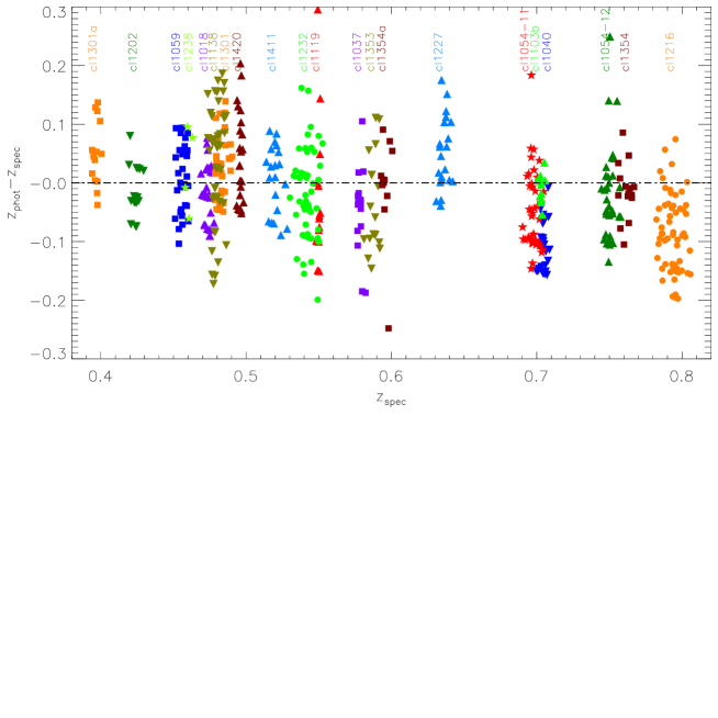
Figure 1: Performance of the photometric redshifts used for the spectroscopic target selection (not the final ones from Pelló et al., in prep.). Plotted are the members of the cluster(s) at the targeted redshift(s) for the given field (21 clusters in 19 fields). For example, if the target selection was $z_{\mathrm{phot}}$ = 0.58$\pm$0.2 for the given field (cf. Table 1), then the $z=0.58$ cluster in that field is plotted, but not the $z=0.43$ cluster. Four galaxies out of 568 are outside the plotted $y$–range. Abbreviated cluster names are given on the plot. The 5 clusters not plotted are cl1037a ($z=0.43$), cl1103a ($z=0.63$), cl1103 ($z=0.96$), cl1138a ($z=0.45$) and cl1227a ($z=0.58$).

The target selection was based on the available VLT/FORS2 optical photometry (White et al. 2005) and the NTT/SOFI NIR photometry (Aragón-Salamanca et al., in prep.). The optical data cover $6.5^{\prime}\times 6.5^{\prime}$ and are well-matched to the FORS2 spectrograph field-of-view. The NIR data cover a somewhat smaller region of $4.2^{\prime}\times 6.0^{\prime}$ (mid–$z$ fields) and $4.2^{\prime}\times 5.4^{\prime}$ (high–$z$ fields). The photometry was used as input to a modified version of the photometric redshifts code hyperz (Bolzonella, Miralles, & Pelló 2000), see also Halliday et al. (2004) and the EDisCS photo–$z$ paper (Pelló et al., in prep.). A combined photometry and photo–$z$ catalogue (hereafter photometric catalogue) used for the target selection, was created for each field prior to each spectroscopic observing run. The aim of the target selection strategy was to keep all galaxies at the cluster redshift (brighter than a certain $I$–band magnitude), while removing objects that were almost certainly not galaxies at the cluster redshift. We will see in Sect. 5 that this aim was successfully achieved. The selection criteria are explained in Halliday et al. (2004). They can be summarised as follows.

1. The I–band magnitude (not corrected for Galactic extinction) within a circular aperture of radius 1^′′, $I_{1}$, had to be in the range $[I_{1,\mathrm{bright}},I_{1,\mathrm{faint}}]$, see Table 1. For the initial short masks (not listed in Table 1) the bright limit was conservatively set to 18.6 for the mid–$z$ fields and 19.5 for the high–$z$ fields, which is about 1 magnitude brighter than the expected magnitude of the brightest cluster galaxy (BCG) (Aragón-Salamanca et al. 1998). For subsequent masks, the bright limit was either kept or set to 0.2 magnitudes brighter than the identified BCG.

2. (a) The best-fit photometric redshift $z_{\mathrm{phot}}$ had to be in the range $[z_{\mathrm{phot,low}},z_{\mathrm{phot,high}}]$ or (b) the $\chi^{2}$-based probability of the best-fit template placed at the estimated or known cluster redshift $z_{\mathrm{cl}}^{\mathrm{P}}$ had to be greater than 50% (see Table 1). The $z_{\mathrm{phot}}$ interval was set to $\pm 0.2$ from the estimated or known cluster redshift. For the long exposures (i.e. those in Table 1), the cluster redshift was usually known from a preceding short exposure (cf. Sect. 2.3). For two fields (1301.7$-$1139 and 1354.2$-$1230), clusters at two redshifts had been identified in the initial short exposure, and here the union of the $\pm 0.2$ intervals was used, giving a wider interval, e.g. $0.60-0.2,0.76+0.2$. The $\pm 0.2$ limit was designed to be fairly conservative: the expectation was that the photo–$z$ dispersion would be 0.1, which would make the selection be $\pm 2\sigma$. The performance of the used photometric redshifts is discussed below.

3. The hyperz star–galaxy separation parameters $N_{\mathrm{gal}}$ and $N_{\ast}$, based on SED fitting minimization, had to have values as follows:
   $N_{\mathrm{gal}}=1$ (“the object could be a galaxy”) or
   $N_{\mathrm{gal}}=2$ (“the object is almost certainly a galaxy”) or
   $N_{\ast}=0$ (“the object is almost certainly not a star”).
   In other words, in the $3\times 3$ grid of $(N_{\mathrm{gal}},N_{\ast})$, the only two grid points not selected are those at (0,1) and (0,2).

4. The FWHM had to be greater than a limit $\mathrm{FWHM}_{\mathrm{min}}$ or the ellipticity $\epsilon$ had to be greater than 0.1, with FWHM and $\epsilon$ being measured in the $I$–band image. This requirement was applied to runs 3 and 4 only. The value of $\mathrm{FWHM}_{\mathrm{min}}$ was determined using 20–30 manually-identified stars in the given field: based on their measured FWHM values, the limit was calculated as $\mathrm{FWHM}_{\mathrm{min}}$ = $\langle$FWHM$\rangle$ + 2$\sigma$(FWHM), with $\langle$FWHM$\rangle$ being the seeing of the image and 2$\sigma$(FWHM) amounting to about 0.1^′′. The value of $\mathrm{FWHM}_{\mathrm{min}}$ was in the range 0.58–0.85^′′ with a typical value of 0.69^′′.

Applying these 4 rules to the photometric catalogue, we derived a target catalogue for the given field and run. Additional constraints of geometrical nature were imposed by the mask design, cf. Sect. 2.2.

Table 1 lists the main target selection parameters for each field and observing run for the 66 long exposure masks. The table does not list the parameters for the short initial masks, since these masks were used only to determine a good guess of the cluster redshift; this observing strategy is described in Sect. 2.3. For reference the table also lists the spectroscopic cluster redshift(s) for the given field derived after all the spectroscopy had been completed. Most fields contain a single main cluster, but a few fields contain one or two secondary clusters in addition to the main cluster; this is discussed in Sect. 4.2.

Having obtained all the spectroscopy, we can check how the photometric redshifts used in the spectroscopic target selection have performed. In Fig. 1 we plot $\Delta z\equiv z_{\mathrm{phot}}-z_{\mathrm{spec}}$ vs $z_{\mathrm{spec}}$ for members of the clusters at the targeted redshifts. The vast majority of the plotted galaxies were selected using rules 1–4 (the exception being serendipitously-observed galaxies; here we have imposed the same magnitude cuts as in rule 1). This implies that Fig. 1 provides a good indication of the photo–$z$ performance for $\Delta z$ in the range $\pm 0.2$. It does not give an unbiased indication of the fraction of ‘catastrophic’ photo–$z$ failures ($|\Delta z|>0.2$); however, that is derived in Sect. 5.2, where the target selection failure rate is found to be about 3%. It is seen from Fig. 1 that the dispersion of $\Delta z$ for the given cluster is quite small, namely in the range 0.03–0.10 (with a typical value 0.06) with the largest value being for cl1138 which at $z=0.48$ would need $B$–band data to achieve a better accuracy. The quoted dispersions are computed as a robust (biweight) estimate. The median value of $\Delta z$ differs somewhat from zero (range $-0.11$ to $+0.07$). This is probably due to minor problems in the photometry used at the time: imperfect photometric zero-points and the lack of seeing-matched photometry. (These problems have been dealt with in the final EDisCS photometric redshifts, Pelló et al., in prep.) When all the clusters are considered together, the dispersion of $\Delta z$ is 0.08 and the median value is $-0.02$.

We can also check the $\chi^{2}$–based probabilities of the best-fit template placed at the cluster redshift used in branch (b) of rule 2. For the photo–$z$ catalogues used in the spectroscopic target selection these probabilities are often too low due to imperfect photometric zero points and the lack of seeing matched photometry. However, since rule 2 has a logical or between branch (a) and (b), and since branch (a) in itself is very good at selecting cluster members, little harm is done by imperfections in branch (b). Furthermore, the inclusion of branch (b) only increased the number of objects in the target catalogues by about 10%, and it made the target selection failure rate be 3% (Sect. 5.2) instead of 5%.

We present now some representative statistics about the number of targets. If we were to apply only the magnitude cuts (i.e. rule 1), the average number of objects per field would be 470 (range 160–860). If we apply the full target selection (i.e. rules 1–4), the average is 260 (range 100–440). The full target selection thus on average rejects almost 50% of the objects that meet the magnitude cuts. The price for this substantial efficiency increase turns out to be missing about 3% of the cluster members (i.e. the failure rate, Sect. 5.2).

To the target catalogues, we added 3 galaxies that did not meet rule 2, since these galaxies had been observed in the initial short mask, and had been found to have redshifts that were close to the estimated cluster redshift. Two of these galaxies were found to be cluster members, and these are counted when computing the failure rate for the target selection for the 66 long masks (Sect. 5.2).

2.2 Automatic creation of the masks

We developed a programme (Poirier 2004) to design the spectroscopic slit masks (called “MXU masks” after the Mask eXchange Unit in the FORS2 spectrograph). A fuller description of how the programme works is found in Halliday et al. (2004); the main points are as follows. The programme starts by placing a slit on the BCG unless it has already been observed in a previous long mask. Slits (10^′′ long) are then placed on objects above and below the BCG. At a given location along the $y$–axis (north–south axis), the brightest object from the target catalogue is chosen (avoiding targets that have already been observed in a previous long mask). Once a slit has been placed at a given location along the $y$–axis, no other slits can be placed at that location (i.e. to the left and right of that slit), since that would cause overlapping spectra. Objects taken from the target catalogue are noted as having targeting flag 1 (cf. Table 2). If no objects from the target catalogue are available at a given location, an object not from the target catalogue is chosen (still imposing a faint magnitude cut in $I_{1}$ of 22 and 23 for mid–$z$ and high–$z$ fields), possibly using a somewhat shorter slit (6–8^′′). These objects acquire a targeting flag 2. Additionally, 2–3 short slits (5^′′) are placed on manually-identified stars. These are used to aid the acquisition and to enable the seeing in the spectral data of a given mask to be accurately measured. These objects are given a targeting flag 4. (All the 108 targeting flag 4 objects observed in the 66 long masks were indeed found to be stars spectroscopically.) Some slits happen to go directly or partially through an object that is not the target. These serendipitously-observed objects are noted as having targeting flag 3.

The achieved wavelength range of the spectra depends on the $x$–location of the slit in the mask. For example, for the runs 3 and 4 setup, a slit at the left, centre and right of the mask would cover an observed-frame wavelength range of approximately 6200–9600 Å, 5200–8500 Å and 4150–7400 Å, respectively. If possible, slits were only placed on objects that were in the $x$–interval that would produce a spectrum that contained the rest-frame wavelength range 3670–4150 Å (covering [OII] and H$\delta$) for the assumed cluster redshift. The width of that $x$–interval depends on the cluster redshift. Slits on stars (targeting flag 4 objects) were not subjected to this restriction.

The masks were inspected, and occasionally objects that had been assigned a slit were removed from the target catalogue and the mask redesigned. This happened in two cases. One was when an object from the photometric catalogue clearly appeared to consist of two distinct physical objects seen partially in projection, but where SExtractor (Bertin & Arnouts 1996) had not been able to deblend them. This seems like a wise choice: in such a situation the photometric redshift (calculated from the combined light of the two physical objects) is meaningless, and it is also not clear on which of the two physical objects to place the slit. The second case was when the object appeared so bright or big that it was perceived to be a foreground field galaxy, which was the case for 10 objects. In retrospect this seems less advisable: 5 of these objects were observed anyway to fill the mask (i.e. as targeting flag 2 objects), and 2 of them did in fact turn out to be cluster members (specifically of cl1059.2$-$1253 at $z=0.46$). The remaining 3 objects were foreground field galaxies, at $z$ = 0.07, 0.35 and 0.46.

The slits were aligned with the major axis of the targeted object if that involved tilting the slit by no more than $\pm 45^{\circ}$. (In run 2, this was only performed for objects that the photometric redshift code identified as late-type galaxies.) Occasionally, when the programme assigned an untilted slit to a target, we manually tilted the slit either to be able to observe a second object ‘serendipitously’ in that slit, or to avoid/reduce signal from very bright, nearby objects.

All slits were 1^′′ wide in the dispersion direction, which means that the spectral resolution for all slits, tilted or not, is practically the same, cf. Sect. 3.5.

Table 2: Targeting flag values

Value	Explanation
1	Targeted as a candidate cluster member
2	Targeted as a field galaxy (filling object)
3	Serendipitous (not targeted)
4	Targeted as a star to aid acquisition and to measure seeing

2.3 Observations

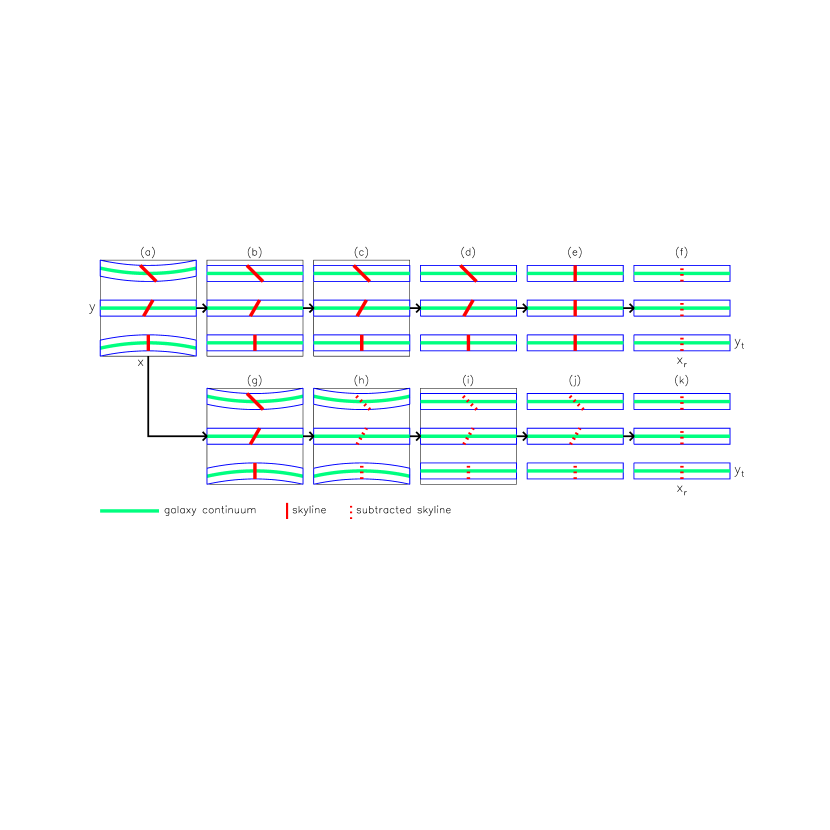
Figure 2: Flowchart for the science frames. The upper branch is for traditional sky subtraction: (a) ‘raw’ frame; (b) after removal of spatial curvature; (c) after flat fielding; (d) after cutting-out the individual spectra; (e) after application of the 2D wavelength calibration; (f) after sky subtraction. The lower branch is for the improved sky subtraction: (a) ‘raw’ frame; (g) after flat fielding; (h) after sky subtraction; (i) after removal of spatial curvature; (j) after cutting out the individual spectra; (k) after application of the 2D wavelength calibration. See text for details. We note that the figure is schematic: it is not to scale, and only 3 spectra per mask (instead of $\sim$30) and 1 skyline per spectrum (instead of $>$100) are shown.

Spectroscopic observations were completed using the FORS2 spectrograph (cf. Appenzeller et al. 1998) on the VLT, during 4 observing runs from 2002 to 2004, spanning 25 nights (22 nights were usable, while 3 nights were lost due to bad weather and technical problems); see Table 1 in Halliday et al. (2004). The same high-efficiency grism was used in all runs (grism 600RI+19, $\lambda_{\mathrm{central}}=6780\,$Å, resolution FWHM $\approx$ 6 Å), but the detector system changed between runs 2 and 3, see Table 2 in Halliday et al. (2004). A total of 86 masks were observed, with 1–6 masks per field; see Table 3 in Halliday et al. (2004), which also lists the exposure times. The typical observing strategy was for a given field to have an initial “short mask” observed in runs 1 or 2, with a total exposure time of typically 0.5–1 hour. Based on the measured redshifts, the confirmed field galaxies and stars were removed from the target catalogue. The objects for which no (secure) redshift could be determined were usually kept in the target catalogue. The confirmed cluster galaxies were given priority so that they almost certainly were included (repeated) in the first “long mask” of that field (typical total exposure time 1–4 hours). For 18 of the 20 EDisCS fields, there are 3–4 (or even 5) long masks per field. For the 1122.9$-$1136 field, no long masks were observed because the initial short mask did not show any convincing cluster (cf. the redshift histogram in Fig. 10). For the 1238.5$-$1144 field, an initial short mask plus a subsequent 20 min mask from run 4 is all that was observed (this field had low priority due to the lack of NIR imaging). The 66 masks listed in the target selection parameter table (Table 1) are the 65 truly long masks plus the 20 min 1238.5$-$1144 mask. The published redshifts (Halliday et al. 2004 and this paper) are practically all from these 66 masks — the data from the 20 initial short masks would only have added a few field galaxies and stars. Data for 5 fields (observed run 2 [mainly] and run 3) were published in Halliday et al. (2004), while data for 14 fields (observed in runs 3 and 4) are published in this paper. No redshifts are published for the 1122.9$-$1136 field, but the few redshifts from the initial short mask are shown in the redshift histogram in Fig. 10.

The 86 masks were exposed for a total of 183 hours (14 hours for the 20 initial short masks and 169 hours for the 66 subsequent long masks). Over the 22 usable nights, this amounts to 8.3 hours of net exposure per night, showing the high efficiency of visitor mode for this type of observations.

In addition to the science observations, various night and day time calibration frames were obtained, see Halliday et al. (2004).

3 Data reduction

This paper describes the data reduction of the runs 3 and 4 data, which amounts to 51 of the 66 long masks listed in Table 1. The reduction was performed using both traditional sky subtraction (Sect. 3.1), and improved sky subtraction (Sect. 3.2). We have adopted the names ‘traditional’ and ‘improved’ sky subtraction for simplicity; more descriptive names would be sky subtraction performed after (respectively before) any rebinning/interpolation of the data has been done.

We note that redshifts based on the traditional reduction for 5 of these 51 masks were included in Halliday et al. (2004). The improved reduction that we have now completed, has no effect on the measurement of redshifts.

3.1 Reduction using traditional sky subtraction

The procedure for the reduction using traditional sky subtraction is described in Halliday et al. (2004), and was developed for previous FORS2 MXU work (Milvang-Jensen 2003; Milvang-Jensen et al. 2003). A summary of the procedure is provided below, and a flowchart for the science frames is shown in the upper branch of Fig. 2.

For a given mask 3–8 individual science frames were usually available. These frames were bias-subtracted and then combined (averaged). At the same time, signal from cosmic-ray hits was removed (cf. Milvang-Jensen 2003; Halliday et al. 2004). Due to the good stability of FORS2, the frame-to-frame shifts in the position of skylines and object continua were so small that the frames could be combined without applying any shifts in $x$ or $y$. This stage is schematically shown in Fig. 2(a). Two features should be noted: (1) The spectra in the upper part of the frame curve like a U and the spectra in the lower part of the frame curve like an upside-down U; this is the spatial curvature or S–distortion. (2) The skylines and the spectral features, in general, are often tilted, because $\sim$50% of the slits in these MXU masks are tilted to be aligned with the major axes of the galaxies (done if the required slit angle was within $\pm 45^{\circ}$).

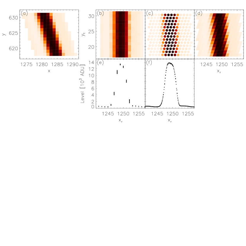
Figure 3: Illustration of the irregular grid. Panels (a) and (b) show regular grids (the type of images usually used in astronomy), i.e. with the data points located at integer-valued coordinate positions. Panel (c) shows an irregular grid, i.e. with the data points located at real-valued coordinate positions. The different panels show: (a) Part of a ‘raw’ frame centered on a bright skyline (no galaxy continuum is present in the shown section), i.e. data that have not been interpolated (rebinned), cf. Fig. 2a. The image is pixelised in $(x,y)$. (b) The same data after interpolation in $y$ to remove spatial curvature and in $x$ to apply the wavelength calibration, cf. Fig. 2e. The image is pixelised in $(x_{\mathrm{r}},y_{\mathrm{t}})$. (c) The exact data values from panel (a), i.e. uninterpolated values, but shown as an irregular grid in $(x_{\mathrm{r}},y_{\mathrm{t}})$ space. (d) Just a different visualisation of the irregular grid in panel (c), corresponding to painting the spectrum in panel (a) on a piece of rubber and stretching it to have axes corresponding to $(x_{\mathrm{r}},y_{\mathrm{t}})$ space. (e) The values from panel (b) plotted versus $x_{\mathrm{r}}$. We note the scatter caused by the interpolation of the sharp edges of the skyline. (f) The values from panel (c) plotted versus $x_{\mathrm{r}}$. We note the very low scatter.

The spatial curvature (S–distortion) was traced from the edges of the $\sim$30 individual spectra in the flat field frames, and removed from the science frames by an interpolation in the $y$–direction (Fig. 2b). The science frames were then flat-fielded (Fig. 2c) and cut-up into the individual spectra (Fig. 2d). The 2D wavelength calibration for each spectrum was established using an arc frame and applied to the science frames using an interpolation in the $x$–direction (Fig. 2e); we note that the skylines are no longer tilted. Each 2D spectrum now has $x_{\mathrm{r}}$ on the abscissa and $y_{\mathrm{t}}$ on the ordinate. The $x_{\mathrm{r}}$ coordinate is linearly related to the wavelength $\lambda$ in Å and the $y_{\mathrm{t}}$ coordinate is linearly related to the spatial position along the slit in arcsec (in the notation of Kelson 2003). We note that our wavelengths are on the air wavelength system (as opposed to the vacuum wavelength system), as is customary for optical work. The sky background could now be fitted and subtracted. The fit was made using pixels in manually-determined sky windows (intervals in $y_{\mathrm{t}}$) which are free from galaxy signal. Finally 1D spectra were extracted from the sky-subtracted 2D spectra. The reduction was performed mainly using IRAF.

3.2 Reduction using improved sky subtraction

The traditional sky subtraction does not work well for spectra produced by tilted slits: strong, systematic residuals are evident where skylines have been subtracted. To remedy this situation, we have implemented a much-improved method for the sky subtraction. The method is described in detail in Kelson (2003). We will follow the notation of Kelson. We have implemented the method from scratch using a combination of IRAF (with TABLES) and IDL.

Figure 3 illustrates a concept central to the method. Panel (a) shows part of a ‘raw’ frame, i.e. data that have not been interpolated (or rebinned; we will use these terms interchangeably), and where the skylines have not been subtracted. The image is pixelised in $(x,y)$, i.e. the image is a regular grid in $(x,y)$. Panel (b) shows what happens in the reduction with traditional sky subtraction: the data, with the skylines still present, have been interpolated in $y$ to remove spatial curvature, and in $x$ to apply the wavelength calibration. The image is pixelised in $(x_{\mathrm{r}},y_{\mathrm{t}})$. These two interpolations are based on analytical mappings (polynomials or spline functions). It is seen that the interpolation of the sharp edges of the skylines has imprinted an aliasing pattern, which prevents a good fit and subsequent subtraction of the skylines. (This aliasing pattern is much more evident once the sky has been subtracted, as will be shown in Fig. 4.) We note that it is the insufficient sampling of the edges of the skylines that is the problem, when performing the sky subtraction in the traditional way (Kelson 2003), not necessarily an undersampling of the skylines. Our data are reasonably well sampled, with the spectral FWHM being sampled by 4 pixels. Panel (c) shows the irregular grid that is central to the improved sky subtraction method. The panel shows the exact uninterpolated data values from panel (a) but as an irregular grid in $(x_{\mathrm{r}},y_{\mathrm{t}})$ space. To turn the regular grid in $(x,y)$ (i.e. panel a) into the irregular grid in $(x_{\mathrm{r}},y_{\mathrm{t}})$ (i.e. panel c), one simply has to use the above-mentioned analytical mappings to compute the correspondence between integer-valued coordinates $(x,y)$ and real-valued coordinates $(x_{\mathrm{r}},y_{\mathrm{t}})$. Panel (d) is just a different visualisation of the irregular grid in panel (c), corresponding to painting the spectrum in panel (a) on a piece of rubber and stretching it to have axes corresponding to $(x_{\mathrm{r}},y_{\mathrm{t}})$ space. To construct this visualisation, one simply has to compute the real-valued $(x_{\mathrm{r}},y_{\mathrm{t}})$ coordinates of the corners of each pixel in the original image (panel a). Panel (e) shows the values from panel (b) plotted versus $x_{\mathrm{r}}$. The before-mentioned aliasing pattern can here be seen as a scatter at a given $x_{\mathrm{r}}$, at the location of the edges of the skyline. Panel (f) shows the values from panel (c) plotted versus $x_{\mathrm{r}}$, and here there is very little scatter.

The essence of the improved sky subtraction method is that the uninterpolated values (for pixels that only contain sky and not object signal) are fitted in the irregular grid in $(x_{\mathrm{r}},y_{\mathrm{t}})$. The fit is subsequently evaluated for the $(x_{\mathrm{r}},y_{\mathrm{t}})$ positions corresponding to all pixel positions in $(x,y)$, i.e. also those containing object signal, and subtracted from the uninterpolated data.

Our implementation of the improved sky subtraction consists of two parts. First, the irregular grid is constructed. In our IRAF-based reduction with traditional sky subtraction, the analytical mappings representing the spatial curvature and the wavelength calibration were established using the tasks identify, reidentify and fitcoords and applied using the task transform, creating an interpolated image. To calculate the coordinates of the irregular grid, these mappings need instead to be evaluated at each integer-valued $(x,y)$ coordinate to determine the corresponding real-valued $(x_{\mathrm{r}},y_{\mathrm{t}})$ coordinate. This task is performed using the task fceval. Second, the irregular grid in $(x_{\mathrm{r}},y_{\mathrm{t}})$ of uninterpolated values are fitted (only for data points located in the manually-determined sky windows, which are intervals in $y_{\mathrm{t}}$). As fitting-functions, we use cubic-splines in $x_{\mathrm{r}}$ and linear polynomials in $y_{\mathrm{t}}$ (similar to the approach taken by Kelson 2003). The node (or breakpoint) spacing of the cubic splines in $x_{\mathrm{r}}$ is denoted $\Delta x_{\mathrm{r}}$. Kelson (2003) was able to obtain a good fit using $\Delta x_{\mathrm{r}}=1$, but we find that this value usually leaves systematic residuals and that $\Delta x_{\mathrm{r}}$ in the range 0.5–0.6 typically is required to achieve a good fit. A node spacing $\Delta x_{\mathrm{r}}$ below one pixel (say $\Delta x_{\mathrm{r}}=0.5$), is not a problem: in many cases the distance between the data points in $x_{\mathrm{r}}$ is much smaller than this (cf. the example in Fig. 3f), and where there are cases of too few data points being located between two adjacent nodes, the software will delete one of the nodes. In most cases a constant function in $y_{\mathrm{t}}$ could have been used instead of a linear one; cf. the example in Fig. 3(f) where any variation in sky level with $y_{\mathrm{t}}$ would have caused the points to scatter, but occasionally a linear function is required to obtain a good fit. The data points are weighted by the inverse of the expected variance. The fitting is done iteratively, and sigma-clipping is applied. We performed the fitting in IDL using modified versions of B–spline procedures written by Scott Burles and David Schlegel, procedures which are part of the idlutils library.

In terms of the flowchart for the science frames (the lower branch in Fig. 2), the reduction proceeds as follows. The starting point is the combined but uninterpolated frame (Fig. 2a). The data are flat-fielded (Fig. 2g), cf. below. The sky is fitted and subtracted as described above (Fig. 2h). The spatial curvature is removed by means of an interpolation in $y$ (Fig. 2i). The individual spectra are cut-out (Fig. 2j). The 2D wavelength calibration is applied by means of an interpolation in $x$ (Fig. 2k), resulting in rectified 2D spectra (i.e. pixelised in $(x_{\mathrm{r}},y_{\mathrm{t}})$) that are sky-subtracted, and with almost no systematic residuals where the skylines have been subtracted. Finally 1D spectra are extracted. We note that all the frames shown in the flowchart are regular grids (normal images). The irregular grid used in fitting the sky, i.e. when going from Fig. 2(g) to Fig. 2(h), is not shown.

As just described, the data are flat-fielded before the sky is fitted, which allows a better fit to be achieved. This in turn implies that an uninterpolated flat field needs to be constructed. The flat field corrects for pixel-to-pixel variations in sensitivity and for the slit profile, i.e. possible variations in light transmission along the slits, e.g. due to the slitwidth not being exactly constant along the slit. The flat field has a level of approximately unity, i.e. there is no variation with wavelength, since the flat field is intended to preserve the counts. This flat field is constructed from the bias-subtracted screen flats (similar to “dome flats”). The wavelength dependence in the screen flats (due to the spectral energy distribution of the used lamp and to the spectral response of the grism, CCD, etc.) is fitted using the same software that is used to fit the sky background, with a large node spacing of $\Delta x_{\mathrm{r}}=50$ in $x_{\mathrm{r}}$ to fit the smooth spectral features in the screen flats, and with constants rather than linear functions in $y_{\mathrm{t}}$ so that the slit profile is not altered. The screen flats are then divided by the fit, creating the desired flat field.

3.3 Comparison of the performance of the two sky subtraction methods

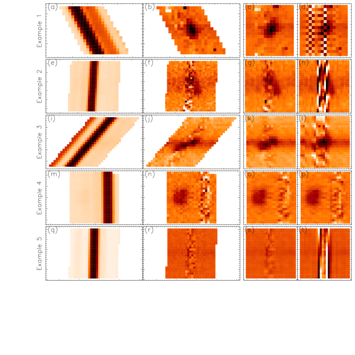
Figure 4: Examples of the results from the improved and the traditional sky subtraction. For each example, we show 4 panels, e.g. (a)–(d). The panels show: (a) ‘Raw’ data (i.e. combined but uninterpolated frame). (b) Sky-subtracted data (improved method), still uninterpolated. (c) Sky-subtracted data (improved method), interpolated (rectified). (d) Sky-subtracted data (traditional method), interpolated (rectified). An identical greyscale is used in panels (b)–(d). We note that all the panels show regular grids. The first two panels (e.g. a and b) are pixelised in $(x,y)$, and the last two panels (e.g. c and d) are pixelised in $(x_{\mathrm{r}},y_{\mathrm{t}})$ and are thus rectified: wavelength is on the abscissa and spatial position is on the ordinate. The greyscale varies from example to example. Examples 1–3 show spectra from tilted slits (slit angles $26.6^{\circ}$, $-3.4^{\circ}$ and $-40.0^{\circ}$, resp.). Examples 4–5 show spectra from untilted slits, but in example 5 the skyline is nevertheless slightly tilted. For spectra with tilted skylines the improved sky subtraction method gives better results than the traditional one. We note that the tilt of the emission lines, seen in the rectified frames in examples 1–3, is due to the rotation of the galaxies. Example 2 shows the [OII] emission line of a $z=0.7$ galaxy, and the corresponding 1D spectrum is shown in Fig. 5(a,b).

Qualitatively, for spectra produced by tilted slits, the improved sky subtraction method is almost always superior to the traditional one. For spectra originating from untilted slits, the two methods provide similar results in most cases. Figure 4 shows 5 examples of the results using the two sky subtraction methods. Panel (a) shows the ‘raw’ spectrum, which has not been rebinned and in which the sky background is still present. Panel (b) shows the immediate result from the improved sky subtraction: a frame that has still not been rebinned, but in which the sky background has been subtracted. Panel (c) shows the rebinned version of panel (b): the spectrum is now rectified and pixelised in $(x_{\mathrm{r}},y_{\mathrm{t}})$. Panel (d) shows the sky-subtracted spectrum from the traditional method (this spectrum is also rectified). The two methods can be directly compared in the two rightmost panels in the figure, e.g. (c) and (d). Examples 1–3 show spectra from tilted slits, and here the traditional method leaves an aliasing pattern (i.e. a systematic error), which the improved method does not. Examples 4–5 show spectra from untilted slits. In example 4, the results from the two methods are similar. In example 5, the skyline is slightly tilted (despite the slit not being tilted), and here the traditional method again leaves an aliasing pattern in the sky-subtracted spectrum.

Figure 5 illustrates the quality improvement of one-dimensional spectra by the improved sky subtraction method in comparison to the traditional one for tilted slits. The residuals of the skylines are significantly reduced for the two typical cluster galaxies shown. For spectral lines of the object falling into the range of strong skylines, this can mean a striking improvement as indicated for [OII] in the case of object 1 (panels a,b) and the G-band in the case of object 2 (panels c,d). The [OII] doublet of object 1 is also shown in the 2D figure (Fig. 4, see example 2).

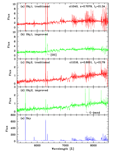
Figure 5: Comparison of the traditional and the improved sky subtraction method for two typical, one-dimensional cluster spectra extracted from tilted slits (slit angles of $-3.4^{\circ}$ and $-40.0^{\circ}$, resp.). The spectra are flux-calibrated and telluric-absorption corrected (see Sect. 3.4). Fluxes are given in units of $10^{-18}\,\mathrm{erg}\,\mathrm{cm}^{-2}\,\mathrm{s}^{-1}\,\mathrm{\AA}^{-1}$. For objects 1 and 2 the significant improvement of [OII] and the G-band, resp., is indicated. The [OII] doublet of object 1 is also shown in Fig. 4 as example 2. The spectra are shown at their native pixel size of 1.6 Å (spectral resolution is 6 Å FWHM) without any smoothing. In order to mark the positions of strong skylines, panel (e) shows a representative sky spectrum.

A quantitative comparison of the results from the two sky subtraction methods is carried out in Appendix A. The main conclusion is that the noise in the improved sky subtraction is very close to the noise floor set by photon noise and read-out noise, whereas the noise in the traditional sky subtraction overall is larger than this (e.g. Fig. 20). This is particularly the case for tilted slits. The difference between the two methods is found where the gradient in the sky background is large, i.e. at the edges of the skylines (Fig. 22, cf. Kelson 2003). For our data, the difference in noise can reach a factor of 10. The difference increases with the total number of collected sky counts, indicating that the longer the total exposure time is, the more of a problem the excess noise in the traditional sky subtraction becomes (Fig. 23).

It should be noted that we have used linear interpolations to perform the rebinning in $y$ and $x$. We have also tested using higher-order interpolations. This makes the aliasing pattern in the traditional sky subtraction somewhat less strong, but the problem is not removed. This indicates that not even a higher-order interpolation can recover the detailed intrinsic shape of the skylines, even though the skylines are not undersampled as such (FWHM $\approx$ 4 pixels). The improved sky subtraction, on the other hand, removes the problem by fitting and subtracting the skylines before any interpolation of the data is done.

3.4 Flux calibration and telluric absorption correction

Spectrophotometric standard stars chosen from the ESO list were observed to be able to flux-calibrate the data, and hot stars (specifically stars with spectral types from O9 to B3, and with magnitude $V$ = 9–10) chosen from the Hipparcos catalogue (ESA 1997) were observed to be able to correct the data for telluric absorption. The star spectra were reduced using standard methods implemented in the long-slit data reduction package ispec2d, which is described in Moustakas & Kennicutt (2006).

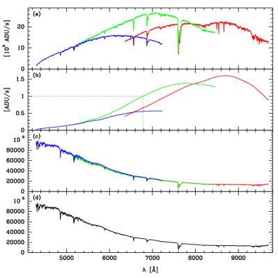
Figure 6: Illustration of the method used to create a flux calibration which is valid for all slit positions. Panel (a) shows 3 spectra of the same star (LTT7379), obtained through slits placed at the extreme right (blue), the centre (green) and the extreme left (red). Panel (b) shows screen flat spectra taken at the same 3 slit positions. The spectral shape has been left untouched, and only the level has been normalised by dividing all 3 spectra by the same constant (cf. the dotted lines; see also the text). Panel (c) shows the star spectra (from panel a) divided by the screen flats (from panel b), i.e. the panel shows the star SED divided by the screen flat lamp SED, a ratio that is used as a tool — the screen flat lamp SED cancels out at the end of the flux calibration procedure. Panel (d) shows the 3 “spectra” from panel (c) merged.

The wavelength range of the individual MXU spectra depends on the $x$–position of the given slit in the MXU mask (cf. Sect. 2.2). To be able to flux-calibrate the full spectral range of all the MXU spectra, we observed spectrophotometric standard stars through slits located at 3 positions: at the far left, at the centre and at the far right. The two extreme positions were chosen to bracket the positions that can be accommodated by the MXU masks. The left, centre and right slits (of width 5^′′) were created using the movable MOS arms of FORS2. When the 3 wavelength-calibrated spectra (i.e. left, centre and right), in units of ADU per second per spectral pixel, of a given star are plotted together, see Fig. 6(a), one problem is immediately clear: the 3 spectra do not agree in the regions in wavelength where the spectra overlap. The disagreement is not just in overall level, but in the shape of the spectra. This means that there is no universal (i.e. valid for all slit positions) function that translates from ADU per second per spectral pixel to physical flux units, e.g. $\mathrm{erg}\,\mathrm{cm}^{-2}\,\mathrm{s}^{-1}\,\mathrm{\AA}^{-1}$. We attribute this to the grism having a spectral response that depends on the position (angle) within the field of view. We use the same solution to this problem as in Halliday et al. (2004). The spectral response of the grism is recorded in all spectra, including in the screen flat spectra (here we are referring to screen flat spectra in which the variation with wavelength has not been taken out, see Fig. 6b and below). We divide both the standard star spectra and the MXU science spectra by their respective screen flats. After that, the left, centre and right standard star spectra agree rather well (Fig. 6c). The 3 spectra can be merged (Fig. 6d), and a sensitivity function can be constructed and then applied to the MXU science spectra that have also been divided by their screen flats, creating flux-calibrated spectra. This method assumes that all screen flats are made using the same lamp, since otherwise the spectral energy distribution (SED) of the screen flat lamp will not cancel out. The screen flats used in the flux calibration only had their overall level normalised: the 3 standard star screen flats (left, centre, right) were normalised by a single number, namely the level in the centre spectrum at 6780 Å (the central wavelength of the grism; cf. Fig. 6b), and the $\sim$30 MXU screen flats from a given mask were normalised by a single number, namely the level in a spectrum from a slit near the centre of the field-of-view at 6780 Å. It should be noted that Fig. 6 is from run 3, where the agreement between the 3 spectra is very good (cf. Fig. 6c). For run 4 the agreement is less good: the spectra are offset in level by $\pm 15$% min–max. We speculate that this is due to a different lamp setup which does not illuminate the 3 slit positions evenly when creating the screen flats. Since we scale the 3 spectra before we merge them (i.e. when going from Fig. 6c to Fig. 6d), no jumps are introduced into the merged spectrum, so the relative flux calibration within a given MXU spectrum is unaffected.

It turns out that 2nd order contamination redwards of 8000 Å is an issue for the flux calibration, but not for the galaxy spectra themselves. From the theory of optics it is known that the different spectral orders of a grism overlap. This implies that the grism transmits light at wavelength $\lambda_{1}$ through the 1st order in the same direction as light at wavelength $\lambda_{2}$ through the 2nd order. For example, light at $\lambda_{1}=$ 7000, 8000 and 9000 Å could be contaminated by light at $\lambda_{2}\approx$ 3700, 4150 and 4600 Å, respectively. This contamination can be prevented by using a filter that blocks light below a certain wavelength $\lambda_{\mathrm{block}}$. In the above example, $\lambda_{\mathrm{block}}$ = 4600 Å would prevent 2nd order contamination until $\lambda_{1}$ = 9000 Å, but it would also prevent 1st order observations below $\lambda_{1}$ = 4600 Å. When the spectral coverage is as large as in our case (4150–9600 Å when all MXU slit positions are considered, Sect. 2.2), the choice of $\lambda_{\mathrm{block}}$ is necessarily a compromise between preventing 2nd order contamination in the red and allowing observations in the blue. We used the order-blocking filter GG435, which is the standard filter to use with grism 600RI. This is an edge filter with a transition around 4350 Å. The listed transmissions are 0.07% at 4100 Å, 3% at 4200 Å and 95% at 4500 Å. Our particular grism also acts as a cross disperser (T. Szeifert, priv. comm.), making the 2nd order spectrum be located 3–4 px (corresponding to 0.75–1^′′) above the 1st order spectrum. This makes it easy to identify the 2nd order spectrum, where present, in the 2D spectra. Figure 7(a) shows part of a raw MXU arc frame. A large number of arc lines are seen in the 1st order spectrum, and two lines are seen in the 2nd order spectrum, displaced upwards by 4 px. Based on three such 2nd order arc lines, a linear fit provides the relation

$$\lambda_{1}=2.0936\lambda_{2}-691.1\,\mathrm{\AA}\enspace,$$ (1)

not unlike relations derived for other grisms (e.g. Szokoly et al. 2004; Stanishev 2007). We only use Eq. (1) to understand from what wavelength a potential 2nd order spectrum would originate. We note that $\lambda_{1}$ = 8000 Å corresponds to $\lambda_{2}$ = 4150 Å, which is just where the order-blocking filter starts to transmit.

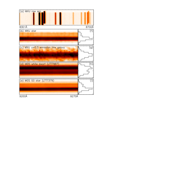
Figure 7: Illustration of 2nd order contamination or lack thereof. (a) Part of a raw MXU arc frame. Most of the lines are from the 1st order, but the 2 lines displaced upwards by 4 px are from the 2nd order. (b)–(e) 2D spectra of four objects. (f)–(i) The corresponding spatial profiles. The figure illustrates that while a modest 2nd order contamination is present (redwards of 8000 Å) in the spectra of the standard star used to establish the flux calibration (LTT7379, panel e), no 2nd order contamination is seen in the galaxy spectra (cf. panel c) due to their redder observed-frame SEDs.

Figure 7 also shows four 2D spectra covering the wavelength range $\lambda_{1}$ = 9200–9270 Å which is in the far red (only 8% of the galaxy spectra go this red). If a 2nd order spectrum is present in the figure, it will come from $\lambda_{2}\approx$ 4720–4760 Å (cf. Eq. 1). Panel (b) shows a somewhat blue star [$(B-V)=0.53,(V-I)=0.81$] observed in one of the MXU masks. A fainter 2nd order spectrum located 4 px above the 1st order spectrum is seen. Panel (c) shows an emission-line galaxy at $z=0.5$. No 2nd order spectrum is seen, presumably due to the redder observed-frame colours. This galaxy has $(V-I)=2.09$, but a more relevant colour would be one that compared 4700 Å to 9200 Å. We note that for galaxies at $z>0.2$ the potential 2nd order contamination comes from below the 4000 Å break in the rest-frame of the galaxy, even at the reddest observed wavelengths (9600 Å). Panel (d) shows a very blue standard star [$(B-V)=0.07$], and here the 2nd order spectrum is dominant. The spacing between the two spectral orders is 3 pixels for the MOS spectra, so even in good seeing the two orders overlap. Panel (e) shows the less blue G0 standard star LTT7379 [$(B-V)=0.62$], which we used to establish the flux calibration. Here a modest 2nd order contamination is present. Figure 7 illustrates two points: (1) A modest 2nd order contamination is found in the used standard star spectra. (2) No significant 2nd order contamination is seen in the galaxy spectra. Point (2) is shown quantitatively below using colours synthesised from the spectra.

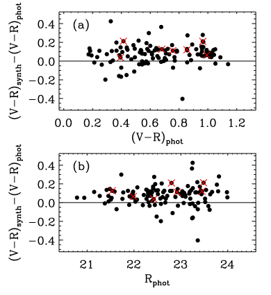
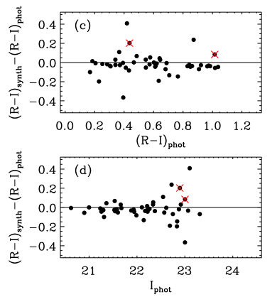
Figure 8: Comparison of colours synthesised from the spectra with colours from the photometry. Panels (a) and (b) concern $(V-R)$, while panels (c) and (d) concern $(R-I)$. To generate this figure, we only used spectra that spanned the wavelength range 4800–7500 Å for panels (a) and (b), and 5700–8700 Å for panels (c) and (d). The different width of these minimum wavelength ranges explains the different number of plotted points. Only galaxies at $z$ = 0.15–1.05 are shown. Only spectra from fields with $VRI$ photometry are used. Most of these are from run 3; the few spectra from run 4 (from 2 masks) are shown with crosses. All colours and magnitudes have been corrected for Galactic extinction and are on the AB system (Oke & Gunn 1983). The photometric colours and magnitudes have been measured within a circular aperture of radius 1^′′ in images corrected to the same fiducial seeing (cf. White et al. 2005). The used transformations to AB are $V_{\mathrm{AB}}=V_{\mathrm{Vega}}+0.036$, $R_{\mathrm{AB}}=R_{\mathrm{Vega}}+0.216$, and $I_{\mathrm{AB}}=I_{\mathrm{Vega}}+0.438$.

In run 3 we observed 7 different standard stars, and in run 4 we observed 2 different standard stars. Typically, one star was observed at the start of the night and another one at the end of the night. There were no indications of night-to-night variations, so for each star all the observations were combined and a sensitivity function was derived. The sensitivity functions for the different stars all agreed until 8000 Å, after which they diverged, with the blue stars (e.g. white dwarfs) indicating a higher sensitivity than the relatively red stars (e.g. G-stars), consistent with the divergence being due to a varying degree of 2nd order contamination. We note that a wide aperture was used to extract 1D spectra, so all the flux from both spectral orders is included. We decided to use the sensitivity function derived from the reddest star observed in both runs, namely the G0 star LTT7379 (Hamuy et al. 1992, 1994; cf. Fig. 6). In the 2D spectrum of this star the 2nd order spectrum is visible from about 8200 Å (cf. the upturn seen in Fig. 6a), so we expect that the calibration is systematically off redwards of 8000 Å by an amount which is modest even at 9200 Å (cf. Fig. 7i). Since we expect the spectra of the high-redshift galaxies to have almost no 2nd order contamination due to their much redder observed-frame SEDs (see also below), a single correction function $f(\lambda)$ valid to a good approximation for all high redshift galaxies should exist. We note that all results published in this paper (e.g. redshifts) are completely unaffected by this issue.

The spectra were corrected for atmospheric extinction. The extinction curve for La Silla was used (Tüg 1977; Schwarz & Melnick 1993) since no extinction curve was available for Paranal (ESO, priv. comm.). This is probably not a problem. The La Silla extinction curve (measured over 41 nights in 1974–1976) can be compared with the Paranal FORS1 broad-band extinction coefficients (measured over 174 nights in 2000–2001) from Patat (2003). At 4300, 5500, 6600 and 7900 Å, which we here take to represent $BVRI$, the La Silla extinction curve gives 0.22, 0.11, 0.05 and 0.02 mag airmass^-1, while the Paranal extinction coefficients are 0.22, 0.11, 0.07 and 0.05 mag airmass^-1 on average, with standard deviations of 0.01–0.02 mag airmass^-1; in other words, a formally perfect agreement for $B$ and $V$, and a systematic difference for $R$ and $I$. The latter is likely due to the extinction curve representing the part of the extinction that varies smoothly with wavelength and which scales accurately with airmass (specifically Rayleigh scattering, ozone absorption and aerosol scattering), but not the telluric absorption bands from oxygen and water vapour present in the $R$ and $I$ bands (Tüg 1977; F. Patat, priv. comm.). This is fortunate, since we will anyway in a separate step correct for the part of the extinction that is due to the telluric absorption bands. That correction is based on spectroscopic observations of hot stars.

Several hot stars were observed. These stars are intrinsically practically featureless in the region where the telluric absorption bands of interest are. Typically 1–2 stars were observed at the start of the night and at the end of the night. A 1^′′ wide longslit was used, giving spectra going to 8600 Å. The continuum was normalised to unity and the spectra from different stars and nights were combined. The spectral regions around the 4 telluric bands present in the hot star data (the B–band near 6900 Å, a weaker feature near 7200 Å, the A–band near 7600 Å, and a weaker feature near 8200 Å) were used to correct the MXU spectra for telluric absorption as follows. For each mask, the spectra of a few bright stars in the mask were located and used to derive the scaling and the shift of the hot star spectrum around the telluric feature in question. The typical rms in these fits was 0.05, as reported by the telluric IRAF task. Each telluric feature was scaled and shifted individually, apart from the weakest band (the one close to 8200 Å), which was locked to the A–band. All the spectra from the given mask were then corrected using this scaled and shifted continuum-normalised hot star spectrum.

As a test of the flux calibration and the two extinction correction steps, we derived synthetic magnitudes from the spectra and compared these with the photometry. The wavelength range of the spectra varies (cf. Sect. 2.2): the bluest spectra start in the middle of the $B$–band and cover the $V$ and $R$–bands, and the reddest spectra start a bit into the $R$–band and end beyond the $I$–band. This means that $(V-R)$ and $(R-I)$ colours can be synthesised from two disjoint subsets of the spectra without extrapolation. The high–$z$ fields with $VRI$ photometry are suited for such a comparison, whereas the mid–$z$ fields with $BVI$ photometry are not. In Fig. 8, we show the results from the comparison. Panel (a) shows the colour difference $(V-R)_{\mathrm{synth}}-(V-R)_{\mathrm{phot}}$ versus the photometric colour, and panel (b) shows the same colour difference versus photometric magnitude. Panels (c) and (d) show $(R-I)$. The scatter in colour difference is fairly small, namely 0.08 mag for $(V-R)$ and 0.06 mag for $(R-I)$, after rejecting 3$\sigma$ outliers. This scatter comes from the following sources: (1) photon noise in the spectra, (2) photon noise in the photometry, (3) possible differences due to the rectangular spectroscopic apertures not being identical to circular photometric apertures, and (4) possible spectrum-to-spectrum errors in the flux calibration. The mean value of the colour difference is $0.08\pm 0.01\,$mag for $(V-R)$ and $-0.03\pm 0.01\,$mag for $(R-I)$. Ideally these values should be zero. We have no explanation for the offset in $(V-R)$, but systematic relative flux calibration uncertainties of the order of 10% are extremely difficult to avoid in multi-slit spectroscopic observations. The negative offset in $(R-I)$ is qualitatively in agreement with the above-mentioned systematic error in the flux calibration redwards of 8000 Å, since part of the $I$–band region of the spectra is located there. It is reassuring to see that there is no significant trend of colour difference with colour (Fig. 8a and c). When a linear fit is performed, the slope is $(0.031\pm 0.026)$ for $(V-R)$ and $(0.001\pm 0.040)$ for $(R-I)$. The fact that the $(R-I)$ slope is consistent with zero is compatible with our conjecture that for high-redshift galaxies, regardless of SED (colour), the 2nd order contamination is negligible. Finally, we have compared the run 3 spectra, which constitute most of the points in Fig. 8, with the run 4 spectra (shown as crosses). The run 4 points tend to lie higher in the plots than the run 3 points, a difference that is marginally significant (2–3 sigma). The difference may be due to the different screen flat lamp setup used in run 4.

Our overall conclusion is that the accuracy of the flux calibration is typically below 10%, which is very good for this type of multi-object spectroscopy. The expected modest systematic error in the flux calibration redwards of 8000 Å can be corrected if it proves necessary.

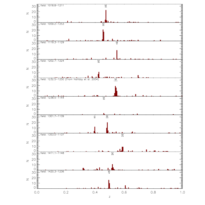
Figure 9: Redshift histograms for the 10 mid–$z$ fields. The clusters for which we have measured a redshift and a velocity dispersion (Halliday et al. 2004 or this paper) are indicated with the $\pm 3\sigma_{\mathrm{cl}}$ range shown. The labels are “M” for the main cluster and “a” or “b” for secondary clusters. Both 0-colon redshifts (“secure”) and 1-colon redshifts (“secure but with larger uncertainties”) have been used in the plot. The binsize in $z$, $\Delta z$, varies with $z$ in such a way that the binsize in rest-frame velocity, $\Delta v_{\rm rest}=c\Delta z/(1+z)$, is kept constant at 1000 km s^-1. This is achieved binning in $\log(1+z)$ space with a constant binsize of $\log(\Delta v_{\rm rest}/c+1)$.

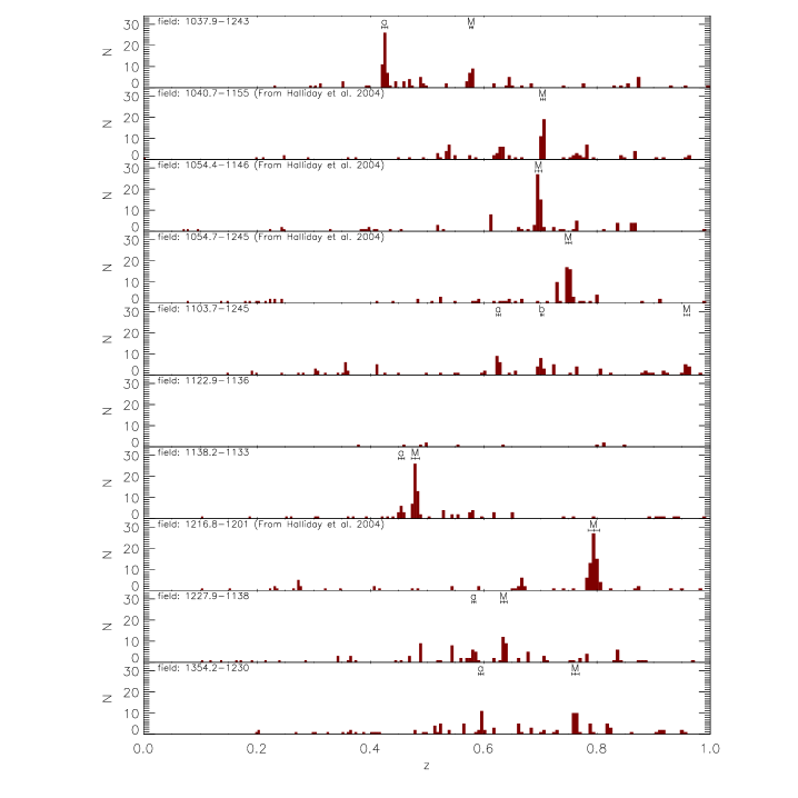
Figure 10: Redshift histograms for the 10 high–$z$ fields. Otherwise this figure is like Fig. 9.

3.5 Test of the wavelength calibration using skylines

To test the wavelength calibration, we measured the wavelength of 3 strong and almost unblended skylines in all the 2D spectra. The reference wavelengths of the 3 lines are 6300.30 Å, 6363.78 Å and 6863.96 Å (Osterbrock et al. 1996), where we have taken into account that the first and the last of these lines are blends of a strong line and a 10–12 times weaker line at our spectral resolution (FWHM $\approx$ 6 Å). For each of the 3 skylines and for each of the $\sim$2000 spectra in the long masks, the difference between the wavelength according to our wavelength calibration and the reference wavelength, $\Delta\lambda\equiv\lambda_{\mathrm{wlcal}}-\lambda_{\mathrm{ref}}$, was calculated. For the 3 lines, the mean values of $\Delta\lambda$ are $-0.11\,$Å, $-0.05\,$Å and $-0.33\,$Å, respectively. The standard deviations are 0.67 Å, 0.67 Å and 0.65 Å, respectively. Since the redshift is given by $z=\lambda_{\mathrm{obs}}/\lambda_{\mathrm{rest}}-1$, and since we typically measure the redshift from spectral lines at wavelengths of approximately $\lambda_{\mathrm{rest}}=3800\,$Å, an error of 0.67 Å in the observed wavelength $\lambda_{\mathrm{obs}}$ translates into an error in the redshift of 0.00018. We note that this number is given with 5 decimals, whereas we normally provide redshifts with only 4 decimals. This error corresponds to a rest-frame velocity of 33 km s^-1, at a typical redshift of $z=0.6$. Since this error is rather small, we have chosen not to correct for it (the zero points of the wavelength calibrations of the individual spectra could in principle have been corrected using the measured values of $\Delta\lambda$). It is worth pointing out that the arc frames from which the wavelength calibrations were established were taken during the day with the telescope pointing at zenith. The fact that the typical error nevertheless is so small testifies to the stability of the FORS2 instrument.

The measurement of the wavelength of the skylines was performed using Gaussian fits. These fits also provide a measure of the width (FWHM) of the lines. For a subset of the masks, we tested how the line width depended on the absolute value of the slit-tilt angle. It was found that there was only a weak dependence: from $0^{\circ}$ to $45^{\circ}$ the FWHM increased on average by just 4%.

4 Galaxy redshifts

4.1 The redshift measurements

Spectroscopic galaxy redshifts were measured using emission lines where possible, in particular the [Oii]$\lambda$3727 line, or the most prominent absorption lines, e.g. Calcium K and H lines at 3934 Å and 3968 Å. The redshifts were manually assigned a quality flag. The vast majority of the measured redshifts are of the highest quality, and these redshifts are listed without colons in our data tables. Secure redshifts but with larger uncertainties are listed with one colon, and doubtful redshifts are listed with two colons. For a small fraction of the objects (3.3%), no redshift could be determined, and these redshifts are listed as 9.9999 in our data tables. For the objects targeted as possible cluster members in the 66 long masks, the statistics are as follows: 2.8% stars, 93.9% galaxies and 3.3% without a determined redshift. Of the galaxy redshifts, the quality distribution (i.e. 0, 1 or 2 colons) is 96.0%, 2.6% and 1.4%, respectively.

We can estimate the typical redshift error using spectra for the galaxies that have been observed more than once (i.e. in more than one mask). In the long masks, we have 43 galaxies with 2 redshifts available, and 2 galaxies with 3 redshifts available, when only using redshifts without colons. For each object and for each redshift, we first compute the difference between the redshift and the mean of the redshifts available for the object. For example, if 2 redshifts of 0.4704 and 0.4708 are available we derive differences of $-0.0002$ and 0.0002; and if 3 redshifts of 0.6960, 0.6962 and 0.6957 are available we get differences of approximately 0.0000, 0.0002 and $-0.0003$. We then divide the differences by 0.7071 for the differences coming from 2 redshifts per object, and by 0.8166 for the differences coming from 3 redshifts per object. These scaling factors were calculated numerically based on a Gaussian distribution. The factors correct for the fact that we calculate the differences with respect to the mean of the observed values, not with respect to the (unknown) mean of the parent distribution. We finally calculate a biweight estimate of the dispersion of the 92 scaled differences, giving 0.00030 (note: 5 decimals) as the estimate of the typical redshift error. This is the same value that was found in Halliday et al. (2004). This error corresponds to 56 km s^-1 in rest-frame velocity at a typical redshift of $z=0.6$.

4.2 Redshift histograms and cluster names

Table 3: IDs for the preliminary BCGs for the additional secondary clusters

Cluster	Alt.	$z_{\mathrm{cl}}$	$z_{\rm BCG}$	BCG ID
Mid–$z$ fields:
cl1301.7$-$1139a	G1_1301	0.3969	0.3976	EDCSNJ1301351$-$1138356
High–$z$ fields:
cl1037.9$-$1243a	…	0.4252	0.4278	EDCSNJ1037523$-$1244490
cl1138.2$-$1133a	C2_1138	0.4548	0.4519	EDCSNJ1138086$-$1136549
cl1227.9$-$1138a	C2_1227	0.5826	0.5812	EDCSNJ1227521$-$1139587
cl1354.2$-$1230a	…	0.5952	0.5947	EDCSNJ1354114$-$1230452

Notes – For the remaining EDisCS clusters the BCG IDs are listed in White et al. (2005). The column “Alt.” gives the name used in Poggianti et al. (2006).

Table 4: Illustration of the format of the spectroscopic catalogues

Object ID	RA (J2000)	Dec (J2000)	$I_{1}$	$z$	Membership flag	Targeting flag
(1)	(2)	(3)	(4)	(5)	(6)	(7)
EDCSNJ1103355$-$1244515	11:03:35.53	$-$12:44:51.5	20.585	0.6259	1a	1
EDCSNJ1103373$-$1246364	11:03:37.34	$-$12:46:36.4	22.051	0.7030	1b	1
EDCSNJ1103420$-$1244409	11:03:41.99	$-$12:44:40.9	22.488	0.9637	1	1
EDCSNJ1103539$-$1248430	11:03:53.85	$-$12:48:43.0	22.556	0.2727	0	2
EDCSNJ1103538$-$1246324	11:03:53.76	$-$12:46:32.4	22.828	0.7539	0	3
EDCSNJ1018371$-$1214297	10:18:37.12	$-$12:14:29.7	19.670	0.0000	–	4
EDCSNJ1103351$-$1249044	11:03:35.12	$-$12:49:04.4	22.938	9.9999	–	1
EDCSNJ1103397$-$1246532	11:03:39.69	$-$12:46:53.2	23.497	0.6246:	1a	3
EDCSNJ1103452$-$1245403	11:03:45.16	$-$12:45:40.3	22.406	0.9383::	0	1
EDCSNJ1227551$-$1136202:A	12:27:55.07	$-$11:36:20.2	21.475	0.6390	1	1
EDCSNJ1227551$-$1136202:B	12:27:55.07	$-$11:36:20.2	21.475	0.5441	0	1
EDCSXJ1103539$-$1244439	11:03:53.91	$-$12:44:43.9	22.63	0.7025	1b	1
EDCSYJ1059032$-$1254311	10:59:03.21	$-$12:54:31.1	99.99	0.4579	1	3

Notes – This example table contains entries from several survey fields simply to illustrate all relevant features of the tables published electronically with this paper, in which the survey fields are not mixed.

Redshift histograms for all 20 EDisCS fields are shown in Fig. 9 (mid–$z$ fields) and Fig. 10 (high–$z$ fields). The binsize in terms of rest-frame velocity is kept constant at 1000 km s^-1 for easier visual interpretation of the histograms. We note that redshift histograms for 5 of the fields (1232.5$-$1250, 1040.7$-$1155, 1054.4$-$1146, 1054.7$-$1245 and 1216.8$-$1201) were already presented in Halliday et al. (2004), but they are repeated here to give an overview of the full set of EDisCS spectroscopy.

On the redshift histogram for the given field, we have indicated the location of the cluster(s) for which we have determined a velocity dispersion in Halliday et al. (2004) or this paper (Sect. 6). Most fields have a single, main cluster. By main cluster is meant the cluster corresponding to the LCDCS detection that our survey originally targeted (cf. White et al. 2005). In some fields there is a secondary cluster labelled “a”, and in one field, there is also an additional secondary cluster labelled “b”. All the main clusters and two of the secondary clusters were already discussed in White et al. (2005). In this paper, we identify 5 additional secondary clusters, chosen so that we have measured a velocity dispersion $\sigma_{\mathrm{cl}}$ of all structures with $\sigma_{\mathrm{cl}}\gtrsim 400$ km s^-1. The naming of the clusters is simple: the main cluster is named “cl” plus the field name (e.g. cl1103.7$-$1245), and the secondary “a” and “b” clusters have that letter added (e.g. cl1103.7$-$1245a, cl1103.7$-$1245b).

In the $xy$ plots and velocity histograms presented in later sections, we indicate the location of the BCG. We therefore need to identify BCGs for the 5 additional secondary clusters. We simply do this by provisionally identifying the brightest (in $I_{\mathrm{tot}}$) spectroscopic member without colons on the redshift as the BCG, see Table 3. We note that the BCGs listed in White et al. (2005) for the other clusters were identified in a more elaborate manner, considering also galaxies for which we only have photometric redshifts. In fact, 3 of the 5 BCGs listed in Table 3 have quite blue colours compared to what is usual for BCGs, making it likely that we simply have not obtained spectroscopy for the true BCG. Conversely, the listed BCGs for the clusters cl1301.7$-$1139a and cl1037.9$-$1243a have colours and total magnitudes in line with the BCGs for the other EDisCS clusters listed in White et al. (2005). These 2 BCGs have been included in the study of the evolution of the EDisCS BCGs (Whiley et al. 2007).

A note should be made about the 1122.9$-$1136 field for which we only have spectroscopy from an initial short mask (plotted in Fig. 10). The galaxy listed in White et al. (2005) as being the BCG and as having $z=0.6397$ does in fact have $z=0.4995$. The few redshifts at hand do not give substantial evidence of a cluster in that field. (The imaging does show some evidence, see White et al. 2005.)

4.3 The spectroscopic catalogues

The spectroscopic catalogues for 5 fields were published in Halliday et al. (2004), and the spectroscopic catalogues for 14 fields are published in this paper. The last of the 20 EDisCS fields has very little data and is not published. The spectroscopic catalogues are published electronically at the CDS. The format of the tables is illustrated in Table 4.

Column 1 gives the object ID. The spectroscopic target selection was based on photometric catalogues created from the imaging available at the time. Subsequently deeper imaging was obtained for some fields (e.g. the total exposure time went from 1 to 2 hours), and new photometric catalogues were created. Both sets of catalogues used the $I$–band image for the object detection and segmentation/deblending (Bertin & Arnouts 1996). For the fields where the $I$–band image had changed due to getting additional data, the object segmentation occasionally differed. For example, a galaxy and a star seen next to each other in projection might have been correctly segmented into two objects in the old catalogue but merged into one object in the new catalogue, or vice versa. The impact is as follows. For 99.5% of the objects targeted and observed spectroscopically the object in the old catalogue is also found in the new catalogue, and here we give the new ID (IDs starting with EDCSNJ). For the remaining 0.5%, the object from the old catalogue is not found in the new catalogue, and here we have constructed IDs starting with EDCSXJ. Additionally, a handful of objects, all non-targeted (i.e. serendipitously observed), neither existed in the old nor in the new catalogues, and we have given these IDs starting with EDCSYJ. We note that the EDCSXJ and the EDCSYJ objects are not found in the published photometric catalogues (e.g. the optical ones from White et al. 2005), since these catalogues are the new ones, but these objects can still be used for purposes that only use the redshift (and position), such as determining cluster velocity dispersions and substructure.

Another issue are the cases where a single object from the photometric catalogue was found to correspond to two physically-distinct objects in the obtained spectrum, i.e. at different redshifts. In the cases where the two redshifts were close we have inspected the available imaging, including HST imaging where available (Desai et al. 2007), to check that it really was two distinct galaxies. For these physically-distinct objects we have constructed unique IDs by appending “:A” and “:B” to the ID from the photometric catalogue (with :A being the southernmost object). We note that in Halliday et al. (2004), where there was one such case, we appended a colon to the IDs for both physical objects instead of :A and :B, resulting in IDs that were not unique, which might be slightly misleading.

Column 2 gives the right ascension, and column 3 gives the declination (J2000).

Column 4 gives $I_{1}$, the I–band magnitude (not corrected for Galactic extinction) within a circular aperture of radius 1^′′. This magnitude comes from the new catalogues (published in White et al. 2005), except for the EDCSXJ objects where it comes from the old catalogues. No magnitude is available for the EDCSYJ objects, and a value of 99.99 is listed in the table.

Column 5 gives the redshift, optionally with one or two colons appended to signify lower quality, see Sect. 4.1. In this paper, the redshifts are always given with 4 decimals. A value of 0.0000 denotes a star, and 9.9999 denotes that no redshift could be determined.

Column 6 gives the membership flag. It is 1 for members of the main cluster, 1a for members of the secondary “a” cluster, 1b for members of the secondary “b” cluster, 0 for field galaxies, and “–” for stars and objects without a determined redshift. The tables for the 14 fields contain flags indicating the 21 clusters listed in Table 5 ahead. Membership is defined as being within $\pm 3\sigma_{\mathrm{cl}}$ from $z_{\mathrm{cl}}$.

Column 7 gives the targeting flag, see Table 2 and Sect. 2.2.

The published redshifts come from the 66 longs masks (i.e. those listed in Table 1). In addition, 9 redshifts from the short initial masks (cf. Sect. 2.3) have been added: 8 galaxies which are members of cl1037.9$-$1243a ($z_{\mathrm{cl}}=0.4252$), and 1 galaxy which is a member of cl1103.7$-$1245 ($z_{\mathrm{cl}}=0.9586$).

As mentioned in Sect. 4.1, some objects were observed more than once. In Halliday et al. (2004), the published tables simply contained all the observations. Here we publish two tables per field: one with one entry per unique object ID, and one table with extra observations. For example, if an object was observed 3 times, we place the best observation in the unique object table, and the two other observations in the extra table. What constitutes the best observation is determined from a set of rules, for example that a redshift with 0 colons has priority over a redshift with 1 colon, and that a targeted observation has priority over a serendipitous observation.

5 Completeness, success rate and potential selection biases

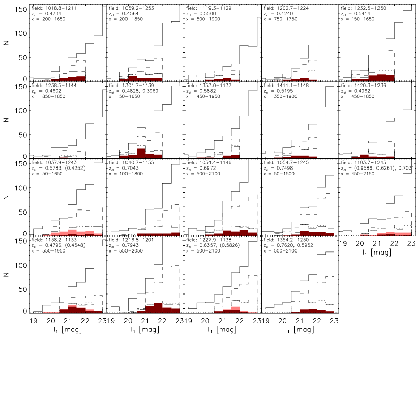
Figure 11: The target selection process as a function of magnitude for the EDisCS fields with long spectroscopic exposures plus the 1238 field. For each panel, the figure shows: solid histogram: objects in the photometric catalogue, dashed histogram: targets, dotted histogram: observed targets, long dashed histogram: targets with a secure redshift, light red filled histogram: galaxies that are members of any cluster in the field (cf. Table 5), dark red filled histogram: galaxies that are members of the cluster(s) at the redshift(s) targeted by the $z_{\mathrm{phot}}$–based target selection. The dotted and the long dashed histograms often coincide, indicating that a secure redshift was obtained for all the observed targets. All numbers have been computed within the region on the sky spanned by the spectroscopic observations, with the range in $x$ being given on the panels, and the range in $y$ being 100–1950 px, cf. the $xy$ plots (Fig. 16). The cluster redshifts are given on the figure. If more than one value is given, the order is: main cluster, secondary cluster “a”, secondary cluster “b”. Values in parentheses are for clusters that are not at the redshift(s) targeted by the $z_{\mathrm{phot}}$–based target selection.

5.1 Completeness and success rate

The target selection process, as a function of $I_{1}$ magnitude, is illustrated in Fig. 11. Each panel corresponds to a given field. To give a complete overview we also show the 5 fields from Halliday et al. (2004). The starting point is a photometric catalogue (solid histogram). Using the 4 target selection rules (Sect. 2.1), the target catalogue is created (dashed histogram). Some of the targets are observed (dotted histogram). For the vast majority of these (95% on average), a secure redshift is obtained (long dashed histogram). Some of these objects are galaxies that are members of any of the clusters in the given field, for which we have measured a velocity dispersion, cf. Table 5 ahead (light red filled histogram). Some galaxies are members of the cluster(s) at the redshift(s) targeted by the $z_{\mathrm{phot}}$–based target selection for the given field (dark red filled histogram). The distinction between the two sets of clusters can be illustrated by the 1037.9$-$1243 field: we have measured a velocity dispersion for both the main cluster (cl1037.9$-$1243, $z_{\mathrm{cl}}=0.58$) and for the secondary “a” cluster (cl1037.9$-$1243a, $z_{\mathrm{cl}}=0.43$). However, the $z_{\mathrm{phot}}$–based target selection only targeted 0.58 (cf. Table 1), i.e. only the main cluster. The cluster redshifts are given on the figure, with the redshifts for the non-targeted clusters being given in parentheses. All the histograms shown in the figure were computed within the region on the sky spanned by the spectroscopic observations. As can be seen from the $xy$ plots in Fig. 16, the objects observed spectroscopically occupy a region which does not span the full width of the imaging. This is done in order to obtain a useful wavelength coverage in the spectra, cf. Sect. 2.2.

Figure 12: The completeness as function of magnitude for the EDisCS fields with long spectroscopic exposures plus the 1238 field. The completeness is defined as $N_{\mathrm{secure}\,z}/N_{\mathrm{targets}}$, with $N_{\mathrm{secure}\,z}$ being the number of targets for which a secure redshift was obtained (long dashed line in Fig. 11), and $N_{\mathrm{targets}}$ being the number of targets (dashed line in Fig. 11). The shown error bars are too large, since they were calculated assuming that the errors on $N_{\mathrm{secure}\,z}$ and $N_{\mathrm{targets}}$ are uncorrelated.

The completeness, here defined as the fraction of the targets for which a secure redshift was obtained, is shown in Fig. 12. The completeness typically decreases as function of magnitude. This happens because the mask-design procedure (Sect. 2.2) gives priority to the brighter objects. When using the spectroscopic sample to study properties that depend on magnitude, such as the incidence of emission lines in the spectra, a correction for the completeness as a function of magnitude can be made using such histograms, cf. Poggianti et al. (2006). It should be noted that Fig. 11 and 12 are based on the published redshift tables (Halliday et al. 2004 and this paper). This means that a few secure redshifts for field galaxies and stars from the initial short masks are not included (cf. Sect. 2.3 and 4.3), so the actual completeness is slightly higher than shown in Fig. 12, particularly at bright magnitudes.

The histograms in Fig. 11 also indicate the success rate of the target selection, i.e. the ratio between the number of galaxies that are members of the cluster(s) at the redshift(s) targeted by the $z_{\mathrm{phot}}$–based target selection (dark red filled histogram) and the number of observed targets (dotted histogram). In terms of the overall success rate (i.e. not as a function of magnitude), for the 21 targeted clusters in all 19 fields with long masks, the success rate is 37% on average, ranging from 12% for the 1103.7$-$1245 field ($z_{\mathrm{cl}}=0.70$), to 63% for the 1301.7$-$1139 field ($z_{\mathrm{cl}}=0.40$, 0.48).

Had we also considered the 5 clusters which happen to be located in the fields but which were not targeted by our $z_{\mathrm{phot}}$–based selection (i.e. the 5 clusters with redshifts given in parentheses on Fig. 11), the success rate would have been 41% on average for the 19 fields, ranging from 21% for the 1238.5$-$1144 field ($z_{\mathrm{cl}}=0.46$), to 64% for the 1138.2–1133 field ($z_{\mathrm{cl}}=0.48$, 0.45). A note should be made about these 5 non-targeted clusters. Three of them (cl1103.7$-$1245a at $z_{\mathrm{cl}}=0.63$, cl1138.2$-$1133a at $z_{\mathrm{cl}}=0.45$, and cl1227.9$-$1138a at $z_{\mathrm{cl}}=0.58$) are at redshifts that are less than 0.1 from the redshifts targeted by the $z_{\mathrm{phot}}$–based selection (cf. Table 1), and any bias in the obtained spectroscopic samples of these clusters is probably small. The remaining two clusters are further than 0.1 from the targeted redshifts: cl1037.9$-$1243a at $z_{\mathrm{cl}}=0.43$, where the selection was $z_{\mathrm{phot}}\in[0.38,0.78]$ (i.e. centered on 0.58), and cl1103.7$-$1245 at $z_{\mathrm{cl}}=0.96$, where the selection was $z_{\mathrm{phot}}\in[0.50,0.90]$ (i.e. centered on 0.70). For the latter cluster in particular, it is possible that the obtained spectroscopic sample is biased with respect to the cluster members as a whole, e.g. in terms of their spectral energy distributions, because the observed sample is one of galaxies at $z_{\mathrm{spec}}=0.96$ for which the photometry gives $z_{\mathrm{phot}}$ in the range 0.50–0.90. For this reason, the spectroscopic samples for those two clusters have not been used in studies of the [OII] emitting galaxies (Poggianti et al. 2006) and the HST–based visual galaxy morphologies (Desai et al. 2007), even though both clusters have interesting properties (a large number of confirmed members and high redshift, respectively).

5.2 Failure rate

As described in Sect. 2.1 the 4 target selection rules were: 1: the magnitude $I_{1}$ had to be in a certain range; 2: the photometric redshift $z_{\mathrm{phot}}$ had to be in a certain range or the probability of being at the cluster redshift had to be greater than 50%; 3: the hyperz galaxy and star flags had to have certain values designed to remove objects that were not galaxies and possibly stars; and 4: the FWHM or the ellipticity had to be greater than certain values designed to remove small and round objects (likely stars; only in runs 3–4). We want to know whether rules 2–4, on top of the simple magnitude selection (rule 1), misses cluster members at the targeted redshifts. We are able to test this because a smaller fraction of the observed objects do not meet the target selection rules — these are objects that were used to fill the masks or which were serendipitously observed. We proceed as follows. In the 66 long masks (cf. Table 1), we select objects that meet rule 1 but not all of rules 2–4. These are 154 (unique) objects. We then remove the 6 objects that we know are blended, i.e. objects with colon-IDs, indicating that a single photometric object turned out to be two spectroscopic objects, typically two galaxies seen in projection (cf. Sect. 4.3). In this situation, the photometric redshift is not meaningful. We also remove the 10 targeting flag 4 objects, i.e. objects that were hand-picked to be stars, and placed into the masks to help field acquisition and to measure seeing. We are left with 138 objects, of which 122 objects (comprised of 102 galaxies and 20 stars) have a measured redshift. Of these 122 objects, 4 are members of the cluster(s) at the targeted redshift(s) for the given field. Therefore, a reasonable estimate of the failure rate of the target selection is 4/122 $\approx$ 3%. Of the 4 failures, 3 failed rule 2. The spectral types of these 3 galaxies differ: one has an absorption-line spectrum, one has an absorption-line spectrum possibly with some emission-filling in H$\beta$, and one has a spectrum with strong emission lines. One galaxy failed rule 3; this galaxy has an absorption-line spectrum. In conclusion, the failure fraction is low (about 3%), and the data for the small number of failures do not indicate that a bias towards a particular spectral type exists. The target selection procedure worked effectively, and for all intents and purposes we expect that our spectroscopic sample of galaxies at the targeted redshifts behaves as an $I$–band selected sample.

6 Cluster redshifts and velocity dispersions

The peculiar velocity of a galaxy with redshift $z$ in the rest-frame of a cluster with redshift $z_{\mathrm{cl}}$ is given by

$$v_{\mathrm{pec}}^{\mathrm{rest}}=c(z-z_{\mathrm{cl}})/(1+z_{\mathrm{cl}})\quad\quad({\rm for}\,\,v_{\mathrm{pec}}^{\mathrm{rest}}\ll c)\enspace$$ (2)

(e.g. Carlberg et al. 1996). The dispersion of the $v_{\mathrm{pec}}^{\mathrm{rest}}$ values for the cluster members is the cluster rest-frame velocity dispersion $\sigma_{\mathrm{cl}}$. Following standard practice, we will omit rest-frame and simply refer to $\sigma_{\mathrm{cl}}$ as the cluster velocity dispersion.

We have tested 2 methods for the determination of $z_{\mathrm{cl}}$ and $\sigma_{\mathrm{cl}}$. The data used in both cases are the set of 0-colon galaxy redshifts available for the given field. Both methods employ an iterative $\pm 3$sigma clipping scheme to determine which galaxies are cluster members. This works as follows. First, initial guesses of $z_{\mathrm{cl}}$ and $\sigma_{\mathrm{cl}}$ are obtained. Then, the following two steps are iterated until convergence on $z_{\mathrm{cl}}$ and $\sigma_{\mathrm{cl}}$ is reached: (1) Calculate $v_{\mathrm{pec}}^{\mathrm{rest}}$ (which depends on $z_{\mathrm{cl}}$) for all the galaxies. (2) For galaxies with $v_{\mathrm{pec}}^{\mathrm{rest}}$ in the interval $[-3\sigma_{\mathrm{cl}},+3\sigma_{\mathrm{cl}}]$, calculate a new estimate of $z_{\mathrm{cl}}$ and $\sigma_{\mathrm{cl}}$. The details of the 2 methods are described below.

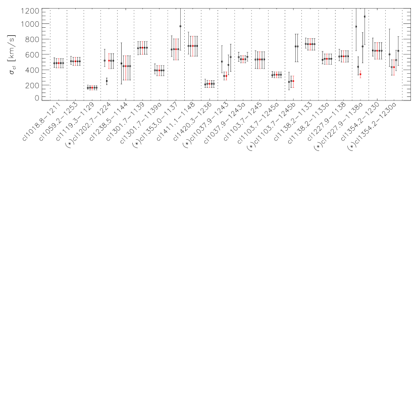
Figure 13: Comparison of the cluster velocity dispersions determined using the 5 methods that we have tested. From left to right for each cluster, the methods are: method 1, method $2_{200}$, method $2_{300}$, method $2_{500}$ and method $2_{1000}$ (see Sect. 6). For most clusters, the results from all methods agree, but for 6 clusters marked with ‘(*)’ this is not the case. For these clusters, the 5 estimates of $\sigma_{\mathrm{cl}}$ are illustrated in Fig. 14.

Method 1 is the method used in our previous paper (Halliday et al. 2004). A first estimate of $z_{\mathrm{cl}}$ is obtained from a visual inspection of the redshift histogram. Galaxies with redshifts outside the region $z_{\mathrm{cl}}\pm 0.015$ are removed and cannot enter the analysis at a later stage. The median redshift of the remaining galaxies is used as a new estimate of $z_{\mathrm{cl}}$, and this value is used to calculate $v_{\mathrm{pec}}^{\mathrm{rest}}$. The standard deviation of the $v_{\mathrm{pec}}^{\mathrm{rest}}$ values is used as the initial estimate of $\sigma_{\mathrm{cl}}$. The iteration then starts, using the median to estimate $z_{\mathrm{cl}}$, and the biweight scale estimator (Beers et al. 1990) to estimate $\sigma_{\mathrm{cl}}$. In the event that the final number of cluster members is below 10, the process is repeated using the gapper scale estimator (Beers et al. 1990) instead of the biweight scale estimator. The 68% asymmetric error bars on $\sigma_{\mathrm{cl}}$ are determined by generating bootstrap samples from the final set of $v_{\mathrm{pec}}^{\mathrm{rest}}$ values for the cluster members. For each bootstrap sample, a value of $\sigma_{\mathrm{cl}}$ is measured without any iterative clipping.

Table 5: Cluster redshifts and velocity dispersions

Cluster	$z_{\mathrm{cl}}$	$\sigma_{\mathrm{cl}}$ [km s-1]	$N_{\mathrm{mem,0}}$	$N_{\mathrm{mem,01}}$	$N_{\mathrm{mem,012}}$
Mid–$z$ fields:
cl1018.8$-$1211	0.4734	$486^{\leavevmode\nobreak\ +59}_{\leavevmode\nobreak\ -63}$	32	32	33
cl1059.2$-$1253	0.4564	$510^{\leavevmode\nobreak\ +52}_{\leavevmode\nobreak\ -56}$	41	41	41
cl1119.3$-$1129	0.5500	$166^{\leavevmode\nobreak\ +27}_{\leavevmode\nobreak\ -29}$	17	17	17
cl1202.7$-$1224	0.4240	$518^{\leavevmode\nobreak\ +92}_{-104}$	19	19	19
cl1238.5$-$1144	0.4602	$447^{+135}_{-181}$	4	4	4
cl1301.7$-$1139	0.4828	$687^{\leavevmode\nobreak\ +81}_{\leavevmode\nobreak\ -86}$	34	35	35
cl1301.7$-$1139a	0.3969	$391^{\leavevmode\nobreak\ +63}_{\leavevmode\nobreak\ -69}$	17	17	17
cl1353.0$-$1137	0.5882	$666^{+136}_{-139}$	18	20	20
cl1411.1$-$1148	0.5195	$710^{+125}_{-133}$	21	22	22
cl1420.3$-$1236	0.4962	$218^{\leavevmode\nobreak\ +43}_{\leavevmode\nobreak\ -50}$	22	24	24
High–$z$ fields:
cl1037.9$-$1243	0.5783	$319^{\leavevmode\nobreak\ +53}_{\leavevmode\nobreak\ -52}$	16	16	16
cl1037.9$-$1243a	0.4252	$537^{\leavevmode\nobreak\ +46}_{\leavevmode\nobreak\ -48}$	43	44	45
cl1103.7$-$1245	0.9586	$534^{+101}_{-120}$	9	10	10
cl1103.7$-$1245a	0.6261	$336^{\leavevmode\nobreak\ +36}_{\leavevmode\nobreak\ -40}$	14	15	15
cl1103.7$-$1245b	0.7031	$252^{\leavevmode\nobreak\ +65}_{\leavevmode\nobreak\ -85}$	11	11	11
cl1138.2$-$1133	0.4796	$732^{\leavevmode\nobreak\ +72}_{\leavevmode\nobreak\ -76}$	45	48	49
cl1138.2$-$1133a	0.4548	$542^{\leavevmode\nobreak\ +63}_{\leavevmode\nobreak\ -71}$	11	12	14
cl1227.9$-$1138	0.6357	$574^{\leavevmode\nobreak\ +72}_{\leavevmode\nobreak\ -75}$	22	22	22
cl1227.9$-$1138a	0.5826	$341^{\leavevmode\nobreak\ +42}_{\leavevmode\nobreak\ -46}$	11	11	11
cl1354.2$-$1230	0.7620	$648^{+105}_{-110}$	20	21	21
cl1354.2$-$1230a	0.5952	$433^{\leavevmode\nobreak\ +95}_{-104}$	14	14	15

Notes – $N_{\mathrm{mem,0}}$ is the number of (unique) cluster members having redshifts without colons (indicating “secure” redshifts). $N_{\mathrm{mem,01}}$ also includes 1-colon redshifts (“secure but with larger uncertainties”). $N_{\mathrm{mem,012}}$ also includes 2-colon redshifts (“not secure”). We note that redshifts and velocity dispersions for 5 additional EDisCS clusters are available in Halliday et al. (2004).

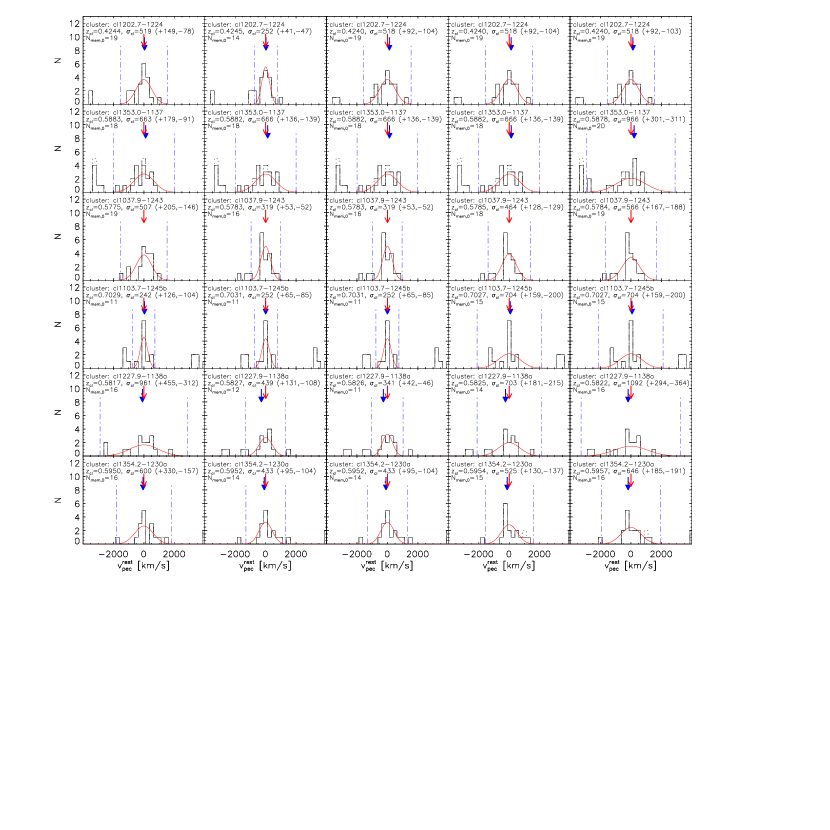
Figure 14: Histograms of peculiar velocities in the cluster rest-frame, $v_{\mathrm{pec}}^{\mathrm{rest}}=c(z-z_{\mathrm{cl}})/(1+z_{\mathrm{cl}})$, for the 6 clusters for which the 5 methods of measuring the cluster redshifts and velocity dispersions do not all agree (cf. Fig. 13). Each row shows a given cluster. We note that all panels in a given row are based on the same redshift data, but since the histograms show $v_{\mathrm{pec}}^{\mathrm{rest}}$ which depends on the cluster redshift $z_{\mathrm{cl}}$, the histograms do not always look completely identical. Each column shows a given method, from left to right: method 1, method $2_{200}$, method $2_{300}$, method $2_{500}$ and method $2_{1000}$. For the analysis we adopt method $2_{300}$. The remaining features of the plots are described in the caption of Fig. 15.

Method 2 uses the final value of $z_{\mathrm{cl}}$ from method 1 as the initial guess of $z_{\mathrm{cl}}$. It uses an initial guess of $\sigma_{\mathrm{cl}}$ of either 200, 300, 500 or 1000 km s^-1, which gives rise to four variants of method 2 referred to as methods $2_{200}$, $2_{300}$, $2_{500}$ and $2_{1000}$. In the iteration, the biweight location estimator (Beers et al. 1990) is used to estimate $z_{\mathrm{cl}}$ and the biweight scale estimator is used to estimate $\sigma_{\mathrm{cl}}$. The 68% asymmetric error bars on $\sigma_{\mathrm{cl}}$ are determined by generating bootstrap samples from the final set of redshifts for the cluster members. Each bootstrap sample is subjected to the same iterative-clipping procedure as the original dataset itself.

The 5 methods were employed on the 21 clusters in the 14 fields. The results in terms of the cluster velocity dispersions are compared in Fig. 13. It is seen that for most clusters the 4 variants of method 2 give identical results (indicating that the initial guess of $\sigma_{\mathrm{cl}}$ has no effect on the result), and the results from method 2 also agree with that from method 1 to within a few per cent. However, for the 6 clusters marked with ‘(*)’ in Fig. 13 not all 5 methods agree. For these clusters the results (i.e. $z_{\mathrm{cl}}$, $\sigma_{\mathrm{cl}}$ and number of cluster members $N_{\mathrm{mem,0}}$) from the 5 methods are illustrated in Fig. 14. This figure shows $v_{\mathrm{pec}}^{\mathrm{rest}}$ histograms calculated for the given value of $z_{\mathrm{cl}}$. The overplotted Gaussians illustrate the given value of $\sigma_{\mathrm{cl}}$, and the vertical dot-dashed lines indicate $\pm 3\sigma_{\mathrm{cl}}$ and hence which galaxies were used in the measurement of $\sigma_{\mathrm{cl}}$ (i.e. the cluster members).

We have inspected the $v_{\mathrm{pec}}^{\mathrm{rest}}$ histograms (Fig. 14) to determine which value of $\sigma_{\mathrm{cl}}$ we consider to be the most “correct” one. For the 6 clusters, our comments are as follows:
cl1202.7$-$1224: Two possible values: $\approx$ 250 and 520 km s^-1. The large value is driven by 4 galaxies on the blue side and 1 galaxy on the red side. These 5 galaxies have a similar location on the plane of the sky to the 14 galaxies in the central velocity peak. Furthermore, the separation in velocity space between the 4 galaxies on the blue side and the 14 galaxies in the central peak is small. This makes us favour the larger value.
cl1353.0$-$1137: Two possible values: $\approx$ 660 and 970 km s^-1. The large value is driven by 2 galaxies which seem to belong to a different peak, which makes us favour the smaller value.
cl1037.9$-$1243: Values range from $\approx$ 320 to 570 km s^-1. The 3 galaxies on the blue side which drive the difference seem somewhat separated in velocity space from the remaining galaxies, which makes us marginally favour the smaller value.
cl1103.7$-$1245b: Two possible values: $\approx$ 250 and 700 km s^-1. The 4 galaxies that drive the difference seem to constitute a separate peak, which makes us favour the smaller value.
cl1227.9$-$1138a: Values range from $\approx$ 340 to 1090 km s^-1. The galaxies that drive the difference seem to constitute several separate peaks, which makes us favour the small value. It was the fact that method 1 gave us the larger value for this particular cluster that made us test the other methods.
cl1354.2$-$1230a: Values range from $\approx$ 430 to 650 km s^-1. Some of the difference is driven by a single galaxy on the blue side which seems quite far from the other galaxies in velocity space. This makes us favour the smaller value.

The conclusion is that method $2_{300}$ — as the only of the tested methods — in all cases provides the result that we consider to be the most “correct” one. We therefore adopt this method throughout the rest of the paper. However, while the method $2_{300}$ results constitute our best guess, the velocity dispersions for these 6 clusters should still be treated as being more uncertain than for the rest of the clusters.

The adopted values of the cluster redshifts, velocity dispersions and number of member galaxies for all 21 clusters in the 14 fields are listed in Table 5. The values of the velocity dispersions are discussed in Sect. 8.

7 Cluster substructure

Possible cluster substructure is investigated using velocity histograms (Sect. 7.1), $xy$ plots (Sect. 7.2) and a Dressler–Shectman analysis (Sect. 7.3).

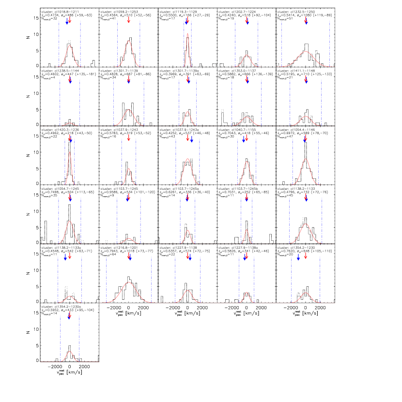
Figure 15: Histograms of peculiar velocities in the cluster rest-frame, $v_{\mathrm{pec}}^{\mathrm{rest}}=c(z-z_{\mathrm{cl}})/(1+z_{\mathrm{cl}})$, for the 26 EDisCS clusters. The solid histograms are for galaxies having redshifts without colons (indicating “secure” redshifts). The dashed histograms include the 1-colon redshifts (“secure but with larger uncertainties”). The dotted histograms include the 2-colon redshifts (“not secure”). The binsize is 250 km s^-1 and the plotted range is $\pm$4000 km s^-1. The overplotted Gaussians illustrate the measured velocity dispersion $\sigma_{\mathrm{cl}}$ of the given cluster. The vertical dot-dashed lines indicate $\pm 3\sigma_{\mathrm{cl}}$, the limits used to define cluster membership. The number of cluster members having redshifts without colons is given as $N_{\mathrm{mem,0}}$, and the area underneath the Gaussian corresponds to this number. The red skeletal arrows are located at $v_{\mathrm{pec}}^{\mathrm{rest}}=0$ km s^-1 and thus indicate the adopted cluster redshifts. The blue filled arrows indicate the adopted BCGs (except where no redshift is available).

7.1 Velocity histograms

Histograms of peculiar velocities in the cluster rest-frame, $v_{\mathrm{pec}}^{\mathrm{rest}}$, are shown for the 26 EDisCS clusters in Fig. 15. These 26 clusters are the ones with a measured velocity dispersion from Halliday et al. (2004) or this paper. The velocity of the BCG is indicated with a blue/filled arrow, except for the 2 BGCs without a spectroscopic redshift (clusters cl1059.2$-$1253 and cl1037.9$-$1243, cf. White et al. 2005). In a few cases, the adopted BCG has a substantial peculiar velocity, e.g. in cl1354.2$-$1230, cf. e.g. Pimbblet et al. (2006). The overplotted Gaussians illustrate the measured velocity dispersions. We note that velocity histograms for 5 of the clusters were already shown in Halliday et al. (2004), but those plots showed observed-frame rather than rest-frame peculiar velocities, whereas the overplotted Gaussians corresponded to the rest-frame velocity dispersions.

From these velocity histograms, most of our clusters appear to be fairly well-described by Gaussian dispersions, particularly those with many members or high velocity dispersions. It is generally unclear whether departures from Gaussianity are real or an effect of limited statistics. One feature that does stand out, however, is the incidence of smaller galaxy associations close to our clusters, which may be due to the tails of the true velocity distribution being longer than Gaussian, but in many cases appear to be separate from the cluster itself. These may be interpreted as groups which surround, and will eventually fall into, the main clusters.

7.2 XY position diagrams

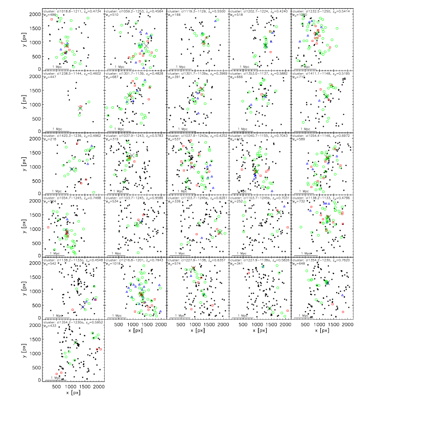
Figure 16: $xy$ plots for the 26 EDisCS clusters. North is up and east is to the left. The units on the axes are pixels = 0.2^′′. Only galaxies with no colons on their redshifts are shown. The small dots are the non-members. The large symbols are the cluster members. Depending on in which bin $v_{\mathrm{pec}}^{\mathrm{rest}}$ falls, the symbols are: blue triangles: $[-3\sigma_{\mathrm{cl}},-1\sigma_{\mathrm{cl}}[$, green circles: $[-1\sigma_{\mathrm{cl}},+1\sigma_{\mathrm{cl}}]$, red squares: $]$$+1\sigma_{\mathrm{cl}},+3\sigma_{\mathrm{cl}}]$. The cross indicates the adopted BCG, which in the case of cl1059.2$-$1253 and cl1037.9$-$1243 does not have any spectroscopy, cf. White et al. (2005). 1 Mpc bars are shown for the assumed cosmology ($\Omega_{\mathrm{m}}=0.3$, $\Omega_{\Lambda}=0.7$ and $H_{0}=70\,\mathrm{km}\,\mathrm{s}^{-1}\,\mathrm{Mpc}^{-1}$).

Plots of the locations of the galaxies on the sky ($xy$ plots) for the 26 EDisCS clusters are shown in Fig. 16. The cluster members are shown with large symbols. The symbol type and colour indicate what bin the peculiar velocity in the rest-frame of the cluster, $v_{\mathrm{pec}}^{\mathrm{rest}}$, falls into. Non-cluster members are shown with small dots. The cross indicates the adopted BCG. One of the 19 main clusters, namely cl1227.9$-$1138, has a BCG that is close to the edge of the field, cf. White et al. (2005). We note that $xy$ plots for 5 of the clusters were already shown in Halliday et al. (2004), but they have been repeated here to provide an overview of the full sample and because the plots here also show the non-cluster members, thus illustrating over which region spectroscopy has been obtained.

For the blended objects where one object in the photometric catalogue turned out to be two physical objects in the spectrum (cf. Sect. 4.3), the two objects (:A and :B) have identical $(x,y)$ coordinates, namely the $(x,y)$ coordinates from the photometric catalogue. To make both objects visible in the $xy$ plot, we have offset the :A object by 1^′′ south and the :B object by 1^′′ north.

The clusters with velocity dispersions $\ga 400\,\mathrm{km}\,\mathrm{s}^{-1}$ generally display a well-defined centre, usually coincident with the BCG. However, several of these clusters show signs of sub-clumps with coherent motion, or possibly even, for cl1216.8$-$1201 and cl1037.9$-$1243a, an overall rotation of the cluster.

7.3 The Dressler–Shectman test

Table 6: Results from the Dressler–Shectman test

Cluster	$z_{\mathrm{cl}}$	$N_{\rm g}$	$\Delta$	$P$
Mid–$z$ fields:
cl1018.8$-$1211	0.4734	$32$	$32.559$	$0.264$
cl1059.2$-$1253	0.4564	$41$	$50.193$	$0.077$
cl1301.7$-$1139	0.4828	$34$	$31.261$	$0.586$
cl1411.1$-$1148	0.5195	$21$	$13.914$	$0.841$
cl1420.3$-$1236	0.4962	$22$	$21.594$	$0.482$
High–$z$ fields:
cl1037.9$-$1243a	0.4252	$43$	$59.027$	$0.010$
cl1138.2$-$1133	0.4796	$45$	$38.456$	$0.631$
cl1227.9$-$1138	0.6357	$22$	$14.428$	$0.782$
cl1354.2$-$1230	0.7620	$20$	$31.260$	$0.001$

Notes – $N_{\rm g}$ is the number of cluster members used in the test ($N_{\rm g}$ is identical to $N_{\mathrm{mem,0}}$ in Table 5), $\Delta$ is the Dressler–Shectman statistic, and $P$ is the probability of there being no substructure in the dataset; thus, a small value (e.g. less than 0.05) indicates that substructure has been detected. We note that Dressler–Shectman results for 5 additional EDisCS clusters are available in Halliday et al. (2004).

     

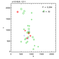
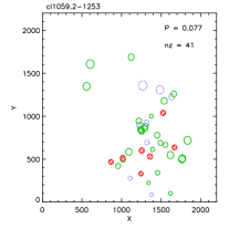
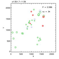
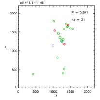
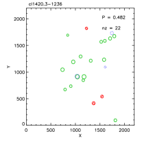
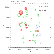
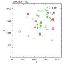
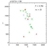
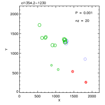
Figure 17: Dressler–Shectman (DS) plots. The DS analysis has only been performed on clusters with at least 20 members. The plots show the $x,y$ location of the cluster members. The radii of the plotted circles are equal to $e^{\frac{\delta}{2}}$ where $\delta$ is the DS measurement of local deviation from the global velocity dispersion and mean recession velocity (cf. Eq. 3). The blue/green/red circles (also shown as dotted/solid/hashed) indicate velocity in the same way as in the $xy$ plots (Fig. 16). The probability $P$ given on the figure is the probability of there being no substructure in the dataset; thus, a small value (e.g. less than 0.05) indicates that substructure has been detected. The number of members is also given on the figure; only redshifts without colons have been used. The 9 clusters in this figure are shown in the same order as in Table 6. We note that DS plots for 5 more clusters are found in Halliday et al. (2004).

In order to check for the presence of substructure in the three-dimensional space, we combine velocity and positional information by computing the statistics devised by Dressler & Shectman (1988). The test works in the following way: for each galaxy that is a spectroscopic cluster member (defined throughout this paper as being within $\pm 3\sigma_{\mathrm{cl}}$ from $z_{\mathrm{cl}}$), the ten nearest neighbours are found, and the local velocity mean and velocity dispersion are computed from this sample of $11$ galaxies. These quantities are compared to the global dynamical parameters computed for the clusters by defining the deviation $\delta$ as:

$$\delta^{2}=(11/\sigma^{2})\left[\left(\bar{v}_{\rm local}-\bar{v}\right)^{2}+\left(\sigma_{\rm local}-\sigma\right)^{2}\right]$$ (3)

where $\bar{v}$ and $\sigma$ are the global dynamical parameters and $\bar{v}_{\rm local}$ and $\sigma_{\rm local}$ are the local mean recessional velocity and velocity dispersion, determined using the $10$ closest galaxies (with spectroscopy available). Velocities and velocity dispersions were transformed to the rest-frame of the cluster.

Dressler & Shectman also define the cumulative deviation $\Delta$ as the sum of the $\delta$ for all the cluster members $N_{\rm g}$. We note that the $\Delta$ statistic is similar to a $\chi^{2}$: if the cluster velocity distribution is close to Gaussian and the local variations are only random fluctuations, then $\Delta$ will be of the order of $N_{\rm g}$.

We have applied the above test to all structures with at least $20$ members, as a conservative compromise between the formal minimum number required to perform the test ($>11$), coupled to the desire to analyse a sample of clusters as large as possible, and the need to find statistically significant substructures. We note that Dressler & Shectman (1988) apply the method to clusters with at least 26 members. The results of such an analysis are shown in Fig. 17. In each panel, the size of the symbols is proportional to $e^{\delta/2}$ and the symbols are coloured according to rest-frame peculiar velocity in the same way as in the $xy$ plots (Fig. 16).

In order to give a quantitative estimate of the significance of substructure, we have performed $1000$ Monte Carlo realizations for each structure by randomly shuffling the velocities of the galaxies used for the analysis. The significance of the occurrence of dynamical substructure can be quantified using the ratio $P$ between the number of simulations in which the value of $\Delta$ is larger than the observed value, and the total number of simulations.

In Table 6 we list, for each of the clusters used in this analysis, the number of spectroscopic members, the measured $\Delta$ statistic, and the probability $P$ of there being no substructure.

Out of the 9 clusters tested in this paper, significant substructure ($P\leq 5\%$) is detected in 2 clusters: cl1037.9$-$1243a at $z=0.43$ ($P=1.0\%$) and cl1354.2$-$1230 at $z=0.76$ ($P=0.1\%$). In Halliday et al. (2004), we tested 5 clusters and detected significant substructure in 2 clusters: cl1232.5$-$1250 at $z=0.54$ ($P=1\%$) and cl1216.8$-$1201 at $z=0.79$ ($P=5\%$). The fraction of EDisCS clusters with detected substructure is 4/14 = 29%. The same level, 21/67 = 31%, was found by Solanes et al. (1999) for a local ($z\la 0.1$) sample of clusters from the ESO Nearby Abell Cluster Survey (ENACS). This sample is also optically-selected, and the same substructure definition was used, i.e. the Dressler & Shectman (1988) test with a $P=5\%$ threshold. More data are required to check this apparent lack of evolution in the fraction of clusters with substructure from $z\sim 0.6$ to $z=0.1$.

8 Discussion

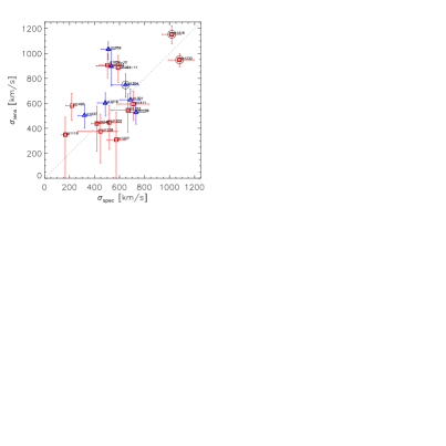
Figure 18: Comparison of the velocity dispersions obtained from the weak lensing analysis (Clowe et al. 2006), $\sigma_{\mathrm{lens}}$, with the velocity dispersions obtained from the spectroscopy (Halliday et al. 2004 and this paper), $\sigma_{\mathrm{spec}}$. The figure shows the 19 main EDisCS clusters ($z$ = 0.42–0.96). The blue triangles are the clusters with other structures near enough to possibly affect the lensing measurements (Clowe et al. 2006), and the red squares are the rest of the clusters. The 3 circled clusters are those for which the Dressler–Shectman test gives a significant detection of substructure (Halliday et al. 2004 and this paper). The dotted line shows the one to one correspondence. Abbreviated cluster names are given on the figure. The 2 major outliers of the blue triangles are cl1059.2$-$1253 and cl1103.7$-$1245, both of which were identified in Clowe et al. (2006) as having extremely high mass-to-light ratios. The 3 major outliers of the red squares are cl1420.3$-$1236, cl1054.7$-$1245 and cl1054.4$-$1146.

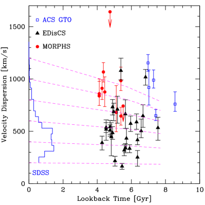
Figure 19: The distribution of velocity dispersion $\sigma$ vs lookback time for EDisCS and for two other well-studied cluster samples at similar redshifts, as well as for a well-studied local sample. The figure shows: SDSS (blue histogram) at $z<0.1$, MORPHS (red circles) at $0.37<z<0.56$, EDisCS (black triangles) at $0.40<z<0.96$, and ACS GTO (blue squares) at $0.8<z<1.3$. The EDisCS clusters fill the gap in lookback time between the MORPHS and the ACS GTO clusters and have a large range in $\sigma$. The dashed lines show how $\sigma$ is expected to evolve with redshift from $z=1$ to $z=0$ (Poggianti et al. 2006). From these curves it is apparent that EDisCS is a high redshift cluster sample for which a majority of the clusters can be progenitors of “typical” low redshift clusters. References for the plotted velocity dispersions: SDSS: von der Linden et al. (2007); MORPHS: Girardi & Mezzetti (2001); EDisCS: Halliday et al. (2004) and this paper; ACS GTO: Gioia et al. (2004); Demarco et al. (2005); Gal & Lubin (2004); Demarco et al. (2004); see also Postman et al. (2005). The shown SDSS sample contains 488 clusters selected to have $\sigma>200\,\mathrm{km}\,\mathrm{s}^{-1}$ and $\sigma/\mathrm{uncertainty}(\sigma)>4$ as measured by von der Linden et al. (2007) for a subset of the C4 cluster sample originally compiled by Miller et al. (2005).

With spectroscopic velocity dispersions, $\sigma_{\mathrm{spec}}$, available for all the EDisCS clusters, we can compare these values with the singular isothermal-sphere velocity dispersions from the weak-lensing analysis from Clowe et al. (2006), $\sigma_{\mathrm{lens}}$. The weak-lensing analysis derived a velocity dispersion for the main cluster in each field, and noted if additional mass peaks were present in the lensing maps. In Fig. 18 we plot $\sigma_{\mathrm{lens}}$ vs $\sigma_{\mathrm{spec}}$ for the 19 main clusters. The blue triangles are the clusters with other structures sufficiently close by in redshift-space, that may directly affect the lensing measurements (Clowe et al. 2006), and the red squares are the rest of the clusters. Visually there is a fairly convincing positive correlation between the two velocity dispersion measurements. Kendall and Spearman rank correlation tests (e.g. Press et al. 1992) lend some support to this: the probability of no correlation comes out to 9% and 4%, respectively. There is no clear offset between the clusters with other peaks in the lensing maps (blue triangles) and the rest of the clusters (red squares). The 3 clusters in the plot with a significant spectroscopic detection of substructure based on the Dressler–Shectman test (probability of no substructure $\leq$ 5%, Halliday et al. 2004 and Sect. 7.3) are indicated with large circles. (The fourth cluster with such a detection, cl1037.9$-$1243a, is not shown in the plot since it is not a main cluster.) One could have expected that $\sigma_{\mathrm{spec}}$ for these clusters would have been higher for their mass (and thus $\sigma_{\mathrm{lens}}$) than for the other clusters, but the limited data in Fig. 18 do not indicate this. This may indicate that the detected substructure does not have a strong effect on the measured spectroscopic velocity dispersions. Of the remaining 16 clusters in the plot, the Dressler–Shectman test does not find significant substructure for 10 of the clusters, and for the last 6 clusters the test has not been performed due to the number of spectroscopic members being less than 20. Among the outliers in the plot the case of cl1103.7$-$1245 can easily be explained: the extra lensing signal is likely due to the secondary cl1103.7$-$1245a cluster to the south. A detailed analysis of the comparison between spectroscopic and lensing velocity dispersions will be presented in Clowe et al., in prep.

The (spectroscopic) velocity dispersions for the EDisCS clusters are generally lower than the velocity dispersions for other well-studied samples of clusters at similar redshifts. This is illustrated in Fig. 19, which plots velocity dispersion versus lookback time for the EDisCS clusters as well as for the MORPHS clusters (e.g. Smail et al. 1997) and the ACS GTO clusters (Postman et al. 2005). The histogram on the left side shows the distribution of the velocity dispersions of a sample of groups and clusters in the SDSS, as described by von der Linden et al. (2007). This sample is based on the C4 cluster sample (Miller et al. 2005), but redefines the cluster centres and velocity dispersions. In particular, the velocity dispersions are computed in a similar fashion to those for the EDisCS sample. The dashed lines show how $\sigma$ is expected to evolve with redshift (Poggianti et al. 2006). From these curves, it is apparent that EDisCS is a high-redshift cluster sample for which a majority of the clusters can be progenitors of “typical” low-redshift clusters.

9 Summary

As part of the ESO Distant Cluster Survey (EDisCS), we have carried out spectroscopic observations with VLT/FORS2 of galaxies in 20 survey fields. In our first paper (Halliday et al. 2004), data for 5 fields were presented, and in this paper we have presented the data for the remaining fields. We have provided details of the target selection procedure, and we have shown how a conservative use of photometric redshifts has given an efficiency increase of almost a factor of 2, while only missing about 3% of the cluster members being targeted. For all intents and purposes, we expect that our spectroscopic sample of galaxies at the targeted redshifts behaves as an $I$–band selected sample. In the data reduction, we have paid particular attention to the sky subtraction. We have implemented the method from Kelson (2003) of performing sky subtraction prior to any rebinning/interpolation of the data. This method delivers photon-noise-limited results, whereas the traditional method of subtracting the sky after the data have been rebinned/interpolated results in substantially larger noise for spectra from tilted slits (about half of our slits are tilted to be along the major axes of the galaxies). The difference between the two methods is found where the gradient in the sky background is large, i.e. at the edges of the skylines (cf. Kelson 2003). For our data, the difference in noise can reach a factor of 10. The difference increases with the total number of collected sky counts, indicating that the longer the total exposure time is, the more of a problem the excess noise in the traditional sky subtraction becomes. We provide data tables containing position, redshifts and $I$–band magnitude for galaxies in 14 fields. Cluster redshifts and velocity dispersions are presented for 21 clusters located in these fields. Together with the clusters from Halliday et al. (2004), velocity dispersions in the range $166\,\mathrm{km}\,\mathrm{s}^{-1}$–$1080\,\mathrm{km}\,\mathrm{s}^{-1}$ are available for 26 EDisCS clusters with redshifts in the range 0.40–0.96. For clusters with at least 20 spectroscopically-confirmed members (9 clusters out of the 21 clusters from this paper), we have performed the Dressler–Shectman test for cluster substructure. Significant detections were obtained for 2 of the clusters. Combined with the results from Halliday et al. (2004) substructure is detected at the 95% confidence level for 4 clusters out of 14 clusters tested. We have taken a first look at the comparison between the velocity dispersions from the weak-lensing analysis (Clowe et al. 2006), and those derived using spectroscopic redshifts. The two quantities show a reasonable agreement. The few clusters with detected substructure do not show an offset from the rest of the clusters, possibly indicating that the detected substructure does not have a strong effect on the measured spectroscopic velocity dispersions. A detailed analysis of the comparison between lensing and spectroscopic velocity dispersions will be presented in a future paper (Clowe et al., in prep.). We have finally noted that the EDisCS clusters, of which many have fairly modest velocity dispersions ($\sim$$500\,\mathrm{km}\,\mathrm{s}^{-1}$), is a high-redshift cluster sample for which a majority of the clusters can be progenitors of “typical” low-redshift clusters.

Therefore, both this property and the large range of masses spanned qualify the EDisCS cluster sample as an unprecedented and unique dataset to study the processes affecting cluster galaxy evolution as a function of cluster mass. Future papers include studies of the optical and NIR luminosity functions, the stellar masses, the stellar populations, the spectral types, the gas phase metallicities, the star formation histories, the dependence of galaxy properties on density, the bar fractions, the Fundamental Plane and the Tully–Fisher relation.

Appendix A Quantitative comparison of the performance of the two sky subtraction methods

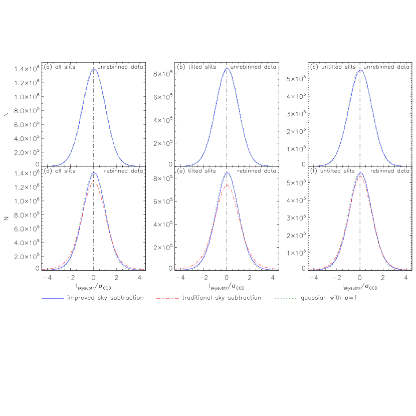
Figure 20: Illustration of the performance of the two sky subtraction methods for the spectra from all the masks and for all wavelengths. The figure shows histograms of $I_{\mathrm{skysubtr}}/\sigma_{\mathrm{CCD}}$, where $I_{\mathrm{skysubtr}}$ are the pixel values in the background-subtracted 2D galaxy spectra, and $\sigma_{\mathrm{CCD}}$ are the corresponding 2D spectra giving the standard deviation expected from the CCD noise model (photon noise and read-out noise; Eq. 4 and 7). Only pixels in the manually determined background regions were used to make the histograms, thus excluding practically all signal from known objects in the spectra (galaxies, stars). The histograms therefore illustrate the scatter caused by both natural noise sources (photon noise and read-out noise) and by possible imperfections in the sky subtraction. Solid/blue histograms: improved sky subtraction (i.e. sky subtraction performed on the unrebinned data); dash-dotted/red histograms: traditional sky subtraction (i.e. sky subtraction performed on the rebinned data). Dotted/green curves: Gaussians with $\sigma=1$, for reference. Panels (a)–(c) show unrebinned data (where sky-subtracted frames are only available for the improved sky subtraction) while panels (d)–(f) show rebinned data (where sky-subtracted frames are available for both types of sky subtraction). Panels (a)+(d) show data from all slits, while the data have been split in tilted and untilted slits in panels (b)+(e) and (c)+(f), respectively. The main conclusions from this figure are: (i) The result from the improved sky subtraction is close to the CCD noise limit, since the data in panel (a) [solid/blue curve] agree so well with a $\sigma=1$ Gaussian [dotted/green curve]; (ii) The improved sky subtraction is better than the traditional one, with a large improvement for tilted slits (panel e) and a smaller improvement for untilted slits (panel f).

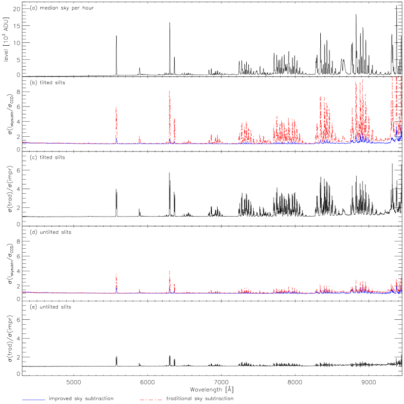
Figure 21: Illustration of the performance of the two sky subtraction methods for the spectra from all the masks as function of wavelength. The data are plotted against wavelength in bins of 1.6 Å. Panel (a) shows a sky spectrum for reference. Panel (b) shows $\sigma(I_{\mathrm{skysubtr}}/\sigma_{\mathrm{CCD}})$, which is the standard deviation of the $I_{\mathrm{skysubtr}}/\sigma_{\mathrm{CCD}}$ values in the given bin. Results from both sky subtraction methods are plotted. A value of 1 represents the noise floor set by photon noise and read-out noise. Panel (c) shows the ratio of $\sigma(I_{\mathrm{skysubtr}}/\sigma_{\mathrm{CCD}})$ for the two methods, illustrating that the traditional sky subtraction has several times more noise than the improved sky subtraction at the locations of skylines. This plot is based on all masks; had we only plotted the masks with the longest exposure times (and hence the largest number of collected sky counts) the difference between the two methods would have been larger. Panels (b) and (c) are for spectra from tilted slits, whereas panels (d) and (e) are for spectra from untilted slits.

To quantify the performance of the two sky subtraction methods (traditional and improved), we will use the values in the sky-subtracted 2D spectra ($I_{\mathrm{skysubtr}}$). We will only use the pixels located in the manually-determined background regions, which are located away from the known objects on the slits. In these regions, there is practically no signal from astronomical objects (galaxies, stars), so in the sky-subtracted spectra the pixel values will scatter around zero. The scatter will come from two sources: “natural” sources found in any CCD frame (photon noise and read-out noise) and possible extra noise from an imperfect subtraction of the skylines. The scatter will vary greatly with wavelength due to the emission-line nature of the sky background spectrum. To normalise things, we will divide the sky-subtracted 2D spectra by the corresponding 2D spectra giving the noise expected from the CCD noise model (photon noise and read-out noise). For uncorrelated pixel values, such as those in the combined but unrebinned (uninterpolated) spectra pixelised in the original coordinates $(x,y)$, the expected noise (in ADU) from the CCD noise model is

$$\sigma_{\mathrm{CCD}}^{\mathrm{unrebinned}}=\sqrt{\frac{I_{\mathrm{non\,skysubtr}}^{\mathrm{unrebinned}}}{n_{\mathrm{ave}}K}+\left(\frac{R_{\mathrm{ADU}}}{\sqrt{n_{\mathrm{ave}}}}\right)^{2}}\quad,$$ (4)

where $I_{\mathrm{non\,skysubtr}}^{\mathrm{unrebinned}}$ (in ADU) represents the combined, non-sky-subtracted 2D spectrum, a spectrum that was created as an average of $n_{\mathrm{ave}}$ individual exposures each with conversion factor $K$ (in e^-/ADU) and read-out noise $R_{\mathrm{ADU}}$ (in ADU). For our dataset, we have $K=0.70\,$e^-/ADU and $R_{\mathrm{ADU}}$ = 4.14 ADU for chip 1, and 4.50 ADU for chip 2.

For the rebinned (interpolated) spectra pixelised in $(x_{\mathrm{r}},y_{\mathrm{t}})$, things are more complicated due to the correlated errors introduced by the interpolations (first in $y$ to remove the spatial curvature, and then in $x$ to apply the 2D wavelength calibration). In principle, one could calculate the expected noise in the rebinned 2D spectrum, $\sigma_{\mathrm{CCD}}^{\mathrm{rebinned}}$, by following how the errors propagate and become correlated through the two interpolations (rebinnings). In practice, this is complicated, so we will take a simpler approach and calculate a quantity $\tilde{\sigma}_{\mathrm{CCD}}^{\mathrm{rebinned}}$ that is equal to $\sigma_{\mathrm{CCD}}^{\mathrm{rebinned}}$ on average and thus equally suitable for statistical comparisons. Imagine two pixels in the unrebinned spectrum, with values $f_{1}$ and $f_{2}$ drawn from identical Gaussian parent distributions with standard deviation $\sigma_{f}$. We do a linear interpolation defined by

$$g=\alpha f_{1}+(1-\alpha)f_{2},\quad 0\leq\alpha\leq 1$$ (5)

to derive the value $g$ in the rebinned pixel. The expected standard deviation of $g$, $\sigma_{g}$, can be calculated from Eq. (5) using the propagation of errors formula for uncorrelated errors, which gives $\sigma_{g}^{2}=\alpha^{2}\sigma_{f}^{2}+(1-\alpha)^{2}\sigma_{f}^{2}$. This reduces to

$$\frac{\sigma_{g}}{\sigma_{f}}=\sqrt{2\alpha^{2}+1-2\alpha}\quad.$$ (6)

This has the following well known consequences: For $\alpha=0$ (i.e. no interpolation), we obtain $\sigma_{g}/\sigma_{f}=1$, meaning that the noise does not change (trivial). And for $\alpha=0.5$ (i.e. taking the average of two values), we obtain $\sigma_{g}/\sigma_{f}=1/\sqrt{2}$, meaning that the noise goes down by a factor of $\sqrt{2}$, at the expense of inheriting correlated errors with the neighbouring pixel. The two values 1 and $1/\sqrt{2}$ are the extremes of Eq. (5). The mean value is found by integrating over $\alpha$ from 0 to 1 and comes out to $\approx$0.81. When we perform another linear interpolation orthogonal to the first one the same arguments apply, and the noise goes down by another factor of $\approx$0.81 on average, i.e. by a factor of $\approx$0.66 in total. The following 2D spectrum

$$\tilde{\sigma}_{\mathrm{CCD}}^{\mathrm{rebinned}}\equiv 0.66\sqrt{\frac{I_{\mathrm{non\,skysubtr}}^{\mathrm{rebinned}}}{n_{\mathrm{ave}}K}+\left(\frac{R_{\mathrm{ADU}}}{\sqrt{n_{\mathrm{ave}}}}\right)^{2}}\quad$$ (7)

will therefore on average provide the correct expected noise in the rebinned spectrum (i.e. when averaging over all the pixels in the spectrum), but for individual pixels the correct factor may not be 0.66 but somewhere between 0.5 and 1.

We note that we are concerned with the expected noise in a single pixel. If we had wanted to calculate the expected noise in, e.g., the sum of the values in a box of $10\times 10$ pixels, the answer would have been different.

In the following, we will simplify the notation and use $\sigma_{\mathrm{CCD}}$ to denote $\sigma_{\mathrm{CCD}}^{\mathrm{unrebinned}}$ (Eq. 4) when dealing with the unrebinned data, and $\tilde{\sigma}_{\mathrm{CCD}}^{\mathrm{rebinned}}$ (Eq. 7) when dealing with the rebinned data.

Our basic quantity for the analysis of the performance of the two sky subtraction methods is $I_{\mathrm{skysubtr}}/\sigma_{\mathrm{CCD}}$ (for pixels in the background regions, which will be implicit from now on). Figure 20 shows histograms $I_{\mathrm{skysubtr}}/\sigma_{\mathrm{CCD}}$. In the first row of panels, the unrebinned data have been used, and here only the improved sky subtraction is available. Also shown are Gaussians with $\sigma=1$, for reference. Panel (a) is for all the slits, whereas panels (b) and (c) shows data from tilted and untilted slits, respectively. The histograms of $I_{\mathrm{skysubtr}}/\sigma_{\mathrm{CCD}}$ in panels (a)–(c) agree very well with the $\sigma=1$ Gaussians, which indicates that the improved sky subtraction is very close to the noise floor set by photon noise and read-out noise. The second row of panels are for the rebinned data. Here we have used the approximate formula for $\sigma_{\mathrm{CCD}}$ (Eq. 7). The histograms for the improved sky subtraction (blue solid histograms) still resemble the $\sigma=1$ Gaussians quite well, indicating that the used approximation is valid on average. For this reason, we will only use the rebinned data in the following figures (Fig. 21–23), since here we can compare the two sky subtraction methods (the traditional sky subtraction is by its nature only available for the rebinned data). The second row of panels of Fig. 20 also show histograms of $I_{\mathrm{skysubtr}}/\sigma_{\mathrm{CCD}}$ for the traditional sky subtraction (red dash-dotted histograms). It is seen that these histograms are wider than those for the improved sky subtraction, showing that the traditional sky subtraction has larger noise than the improved sky subtraction. This is particularly the case for spectra coming from tilted slits (panel e), as expected.

Figure 21 plots $I_{\mathrm{skysubtr}}/\sigma_{\mathrm{CCD}}$ in a different way. The data are split in bins of 1.6 Å in wavelength. Instead of plotting a histogram of the $I_{\mathrm{skysubtr}}/\sigma_{\mathrm{CCD}}$ values, a robust (biweight) estimate of their standard deviation, $\sigma(I_{\mathrm{skysubtr}}/\sigma_{\mathrm{CCD}})$, is calculated and plotted versus wavelength, see panel (b) (tilted slits) and (d) (untilted slits). The results from both sky subtraction methods are plotted, and their ratio is plotted in panels (c) and (e). Panel (a) shows a sky spectrum for reference, and it is seen that the traditional sky subtraction has several times larger noise than the improved sky subtraction at the location of the skylines. It is also seen that this difference in noise increases with the strength of the skyline. This indicates that the extra noise found in the traditional sky subtraction is a stronger function of the sky level than the square root which enters $\sigma_{\mathrm{CCD}}$ (Eq. 7).

Figure 22 is akin to a zoom of Fig. 21 centered at the strong 6300 Å skyline. The figure shows that the traditional sky subtraction method has the highest noise at the edges of the skylines, i.e. where the gradient in the sky background is the largest (cf. Kelson 2003). Panel (c) shows that for tilted slits in this particular mask the noise in the traditional sky subtraction is 7–8 times larger than the noise in the improved sky subtraction at the edges of this skyline.

Figure 23 shows $\sigma(I_{\mathrm{skysubtr}}/\sigma_{\mathrm{CCD}})$ versus the number of collected sky counts for both sky subtraction methods and for tilted slits (panel a) and untilted slits (panel b). As before, the quantity $\sigma(I_{\mathrm{skysubtr}}/\sigma_{\mathrm{CCD}})$ would be unity if the noise in the sky-subtracted spectra was at the noise floor set by photon noise and read-out noise. What is seen most clearly in panel (a) is that the improved sky subtraction (blue crosses) is almost at the noise floor, with just a small excess noise that increases weakly with the number of collected sky counts. The traditional sky subtraction (red triangles) is much above the noise floor, and $\sigma(I_{\mathrm{skysubtr}}/\sigma_{\mathrm{CCD}})$ increases with the number of collected sky counts in a way resembling a square root function. Since $\sigma(I_{\mathrm{skysubtr}}/\sigma_{\mathrm{CCD}})$ has already been divided by $\sigma_{\mathrm{CCD}}$ (which essentially is proportional to the square root of the number of collected sky counts), the plot indicates that the extra noise in the traditional sky subtraction goes linearly with the number of collected sky counts. This has the implication that for increasingly long total exposure times, the systematic extra noise in the traditional sky subtraction becomes larger and larger compared to the photon noise.

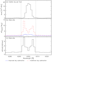
Figure 22: Illustration of the fact that the traditional sky subtraction method has the highest noise at the edges of the skylines, i.e. where the gradient in the sky background is the largest (cf. Kelson 2003). This figure is akin to a zoom of Fig. 21 centered at the strong 6300 Å skyline, but only data from a single mask have been used (and we note that the $y$–axis range for panel b has been increased). If this figure had been made using all 51 masks it would have looked rather similar, but the peaks in panel (b) and (c) would not have been so sharp due to the small wavelength shifts that exist between the masks due to instrument flexure. The dotted lines indicate the wavelength region used for the statistics shown in Fig. 23.

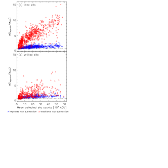
Figure 23: Illustration of how the noise in the sky-subtracted spectra depends on the collected sky counts. Only data in the narrow wavelength range $6300\pm 8\,$Å have been used (cf. Fig. 22). Data from all 51 masks have been used. The $x$–axis shows the mean collected sky counts over the total exposure time for the given spectrum, with the mean being taken over the used wavelength range. The quantity on the $x$–axis thus depends linearly on the total exposure time and on the sky brightness at 6300 Å. The $y$–axis shows $\sigma(I_{\mathrm{skysubtr}}/\sigma_{\mathrm{CCD}})$ which was also used in Fig. 21 and 22, just here computed in the single wavelength bin of $6300\pm 8\,$Å instead of in multiple bins of 1.6 Å. The quantity on the $y$–axis is the noise relative to $\sigma_{\mathrm{CCD}}$ (the noise expected from photon noise and read-out noise). The horizontal dot–dashed line at 1 represents the noise floor set by photon noise and read-out noise. The points for the traditional sky subtraction show a square root like behaviour. Since the quantity on the $y$–axis has already been divided by $\sigma_{\mathrm{CCD}}$ (which essentially is proportional to the square root of the quantity on the $x$–axis) the plot indicates that the extra noise in the traditional sky subtraction goes linearly with the number of collected sky counts.