Improved Constraints on the Preferential Heating and Acceleration of Oxygen Ions in the Extended Solar Corona

Abstract

We present a detailed analysis of oxygen ion velocity distributions in the extended solar corona, based on observations made with the Ultraviolet Coronagraph Spectrometer (UVCS) on the SOHO spacecraft. Polar coronal holes at solar minimum are known to exhibit broad line widths and unusual intensity ratios of the O VI $\lambda\lambda$1032, 1037 emission line doublet. The traditional interpretation of these features has been that oxygen ions have a strong temperature anisotropy, with the temperature perpendicular to the magnetic field being much larger than the temperature parallel to the field. However, recent work by Raouafi and Solanki suggested that it may be possible to model the observations using an isotropic velocity distribution. In this paper we analyze an expanded data set to show that the original interpretation of an anisotropic distribution is the only one that is fully consistent with the observations. It is necessary to search the full range of ion plasma parameters to determine the values with the highest probability of agreement with the UVCS data. The derived ion outflow speeds and perpendicular kinetic temperatures are consistent with earlier results, and there continues to be strong evidence for preferential ion heating and acceleration with respect to hydrogen. At heliocentric heights above 2.1 solar radii, every UVCS data point is more consistent with an anisotropic distribution than with an isotropic distribution. At heights above 3 solar radii, the exact probability of isotropy depends on the electron density chosen to simulate the line-of-sight distribution of O VI emissivity. The most realistic electron densities (which decrease steeply from 3 to 6 solar radii) produce the lowest probabilities of isotropy and most-probable temperature anisotropy ratios that exceed 10. We also use UVCS O VI absolute intensities to compute the frozen-in O⁵⁺ ion concentration in the extended corona; the resulting range of values is roughly consistent with recent downward revisions in the oxygen abundance.

1. Introduction

The physical processes that heat the solar corona and accelerate the solar wind are not yet understood completely. In order to construct and test theoretical models, there must exist accurate measurements of relevant plasma parameters in the regions that are being heated and accelerated. In the low-density, open-field regions that reach into interplanetary space, the number of plasma parameters that need to be measured increases because the plasma begins to become collisionless and individual particle species (e.g., protons, electrons, and heavy ions) can exhibit different properties. Such differences in particle velocity distributions are valuable probes of “microscopic” processes of heating and acceleration. The Ultraviolet Coronagraph Spectrometer (UVCS) operating aboard the Solar and Heliospheric Observatory (SOHO) spacecraft has measured these properties for a variety of open-field regions in the extended corona (Kohl et al.  1995, 1997, 2006).

In this paper we focus on UVCS observations of heavy ion emission lines (specifically O VI $\lambda\lambda$1032, 1037) in polar coronal holes at solar minimum. One main goal is to resolve a recent question that has arisen regarding the existence of anisotropic ion temperatures in polar coronal holes. Several prior analyses of UVCS data have concluded that there must be both intense preferential heating of the O⁵⁺ ions, in comparison to hydrogen, and a strong field-aligned anisotropy with a much larger temperature in the direction perpendicular to the magnetic field than in the parallel direction (see, e.g., Kohl et al.  1997, 1998; Li et al.  1998; Cranmer et al.  1999; Antonucci et al.  2000; Zangrilli et al.  2002; Antonucci 2006; Telloni et al.  2007). However, Raouafi & Solanki (2004, 2006) and Raouafi et al.  (2007) have reported that there may not be a compelling need for O⁵⁺ anisotropy depending on the assumptions made about the other plasma properties of the coronal hole (e.g., electron density).

The determination of O⁵⁺ preferential heating, preferential acceleration, and temperature anisotropy has spurred a great deal of theoretical work (see reviews by Hollweg & Isenberg 2002; Cranmer 2002a; Marsch 2005; Kohl et al.  2006). It is thus important to resolve the question of whether these plasma properties are definitively present on the basis of the UVCS/SOHO observations. In this paper, we attempt to analyze all possible combinations of O⁵⁺ properties (number density, outflow speed, parallel temperature, and perpendicular temperature) with the full effects of the extended line of sight (LOS) taken into account. The applicability of any particular combination of ion properties is evaluated by computing a quantitative probability of agreement between the modeled set of emission lines and a given observation. Preliminary results from this work were presented by Cranmer et al.  (2005) and Kohl et al.  (2006).

The original UVCS results of preferential ion heating and acceleration—as well as strong ion temperature anisotropy ($T_{\perp}\gg T_{\parallel}$)—were somewhat surprising, but these extreme departures from thermal equilibrium are qualitatively similar to conditions that have been measured for decades in high-speed streams in the heliosphere. At their closest approaches to the Sun ($\sim$ 0.3 AU), the Helios probes measured substantial proton temperature anisotropies with $T_{\perp}>T_{\parallel}$ (Marsch et al.  1982; Feldman & Marsch 1997). In the fast wind, most ion species also appear to flow faster than the protons by about an Alfvén speed ($V_{A}$), and this velocity difference decreases with increasing radius and decreasing proton flow velocity (e.g., Hefti et al.  1998; Reisenfeld et al.  2001). The temperatures of heavy ions are significantly larger than proton and electron core temperatures. In the highest-speed wind streams, ion temperatures exceed simple mass proportionality with protons (i.e., heavier ions have larger most-probable speeds), with $(T_{\rm ion}/T_{p})>(m_{\rm ion}/m_{p})$, for $m_{\rm ion}>m_{p}$ (e.g., Collier et al.  1996). UVCS provided the first evidence that these plasma properties are already present near the Sun.

The outline of this paper is as follows. In § 2 we present an expanded collection of UVCS/SOHO observational data that is used to determine the O⁵⁺ ion properties. § 3 outlines the procedure we have developed to produce empirical models of the plasma conditions in polar coronal holes and to compute the probability of agreement between any given set of ion properties and the observations. The resulting ranges of ion properties that are consistent with the UVCS observations are presented in § 4 along with, in our view, a resolution of the controversy regarding the oxygen temperature anisotropy. Finally, § 5 gives a summary of the major results of this paper and a discussion of the implications these results may have on theoretical models of coronal heating and solar wind acceleration.

2. Observations

The UVCS instrument contains three reflecting telescopes that feed two ultraviolet toric-grating spectrometers and one visible light polarimeter (Kohl et al.  1995, 1997). Light from the bright solar disk is blocked by external and internal occulters that have the same linear geometry as the spectrometer slits. The slits are oriented in the direction tangent to the solar limb. They can be positioned in heliocentric radius $r$ anywhere between about 1.4 and 10 solar radii ($R_{\odot}$) and rotated around the Sun in position angle. The slit length projected on the sky is 40′, or approximately 2.5 $R_{\odot}$ in the corona, and the slit width can be adjusted to optimize the desired spectral resolution and count rate.

The UVCS data discussed in this paper consist of a large ensemble of observations of polar coronal holes from the last solar minimum (1996–1997). The solar magnetic field is observed to exist in a nearly axisymmetric configuration at solar minimum, with open field lines emerging from the north and south polar regions and expanding superradially to fill a large fraction of the heliospheric volume. The plasma properties in polar coronal holes remain reasonably constant in the year or two around solar minimum (see, e.g., Kohl et al.  2006), so we assemble the data over this time into a single function of radius. In this paper, we limit ourselves to the analysis of observations of the O VI $\lambda\lambda$1032, 1037 emission line doublet in these polar regions. The relevant UVCS observations are taken from the following three sources.

1. The empirical model study of Kohl et al.  (1998) and Cranmer et al.  (1999) covered the period between 1996 November and 1997 April and took the north and south polar coronal hole properties to be similar enough to treat them together.

2. A detailed analysis of the north polar coronal hole by Antonucci et al.  (2000) coincided with the second SOHO joint observing program (JOP 2) on 1996 May 21.

3. We searched the UVCS/SOHO archive for any other north or south polar hole observations having sufficient count-rate statistics to be able to measure the O VI line widths at radii above 2 $R_{\odot}$. A total of 14 new or reanalyzed data points were identified between 1996 June and 1997 July.

The remainder of this section describes the data reduction for the third group of new data points. Table 1 provides details of these 14 measurements.

Table 1Newly Analyzed Polar Coronal Hole Data: 1996–1997

Start Date, UT Time	Obs.  Height	Slit Length	Slit Width	Exposure	$V_{1/e}$	${\cal R}$	$I_{\rm tot}$, 1032 Å line
	($R_{\odot}$)	(arcmin)	($\mu$m)	Time (hr)	(km s-1)		(106 phot s-1 cm-2 sr-1)
1996 Jun 21, 16:55	2.07	15.8 (N)	75	9.1	$363\pm 21.7$	$2.09\pm 0.4$	$32.2\pm 6.8$
1996 Sep 29, 15:26	2.08	17.5 (N)	75	5.6	$473\pm 12.4$	$1.87\pm 0.14$	$43.2\pm 8.7$
1996 Nov 07, 23:38	2.07	29.7 (N)	75	7.6	$409\pm 18.8$	$1.78\pm 0.2$	$44.6\pm 9.1$
1996 Nov 10, 06:30	3.00	25.7 (N)	350	9.4	$475\pm 27.0$	$1.16\pm 0.18$	$2.08\pm 0.44$
1996 Nov 10, 15:55	2.56	25.9 (N)	350	10.8	$505\pm 30.5$	$1.17\pm 0.17$	$4.83\pm 1.0$
1996 Nov 16, 16:56	2.17	29.6 (N)	340	9.5	$417\pm 7.43$	$1.485\pm 0.06$	$25.1\pm 5.0$
1997 Jan 05, 21:00	3.07	28.0 (N)	100	17.6	$690\pm 87.2$	$0.957\pm 0.45$	$2.02\pm 0.63$
1997 Jan 10, 14:54	3.08	20.8 (N)	150	68.8	$686\pm 38.7$	$1.23\pm 0.3$	$3.37\pm 0.76$
1997 Jan 24, 16:03	3.08	20.6 (N)	150	70.8	$594\pm 41.6$	$1.01\pm 0.3$	$1.66\pm 0.40$
1997 Mar 09, 18:00	2.57	19.0 (S)	300	8.9	$500\pm 22.0$	$1.15\pm 0.12$	$5.66\pm 1.2$
1997 Jun 04, 16:49	2.56	18.8 (N)	300	9.0	$527\pm 33.9$	$0.958\pm 0.15$	$4.14\pm 0.90$
1997 Jun 08, 20:15	3.10	18.7 (N)	300	8.3	$645\pm 65.6$	$1.33\pm 0.44$	$1.33\pm 0.33$
1997 Jul 01, 15:50	2.56	17.2 (N)	342	9.8	$534\pm 56.8$	$0.988\pm 0.26$	$3.26\pm 0.80$
1997 Jul 04, 16:45	3.63	18.9 (N)	342	29.5	$451\pm 47.9$	$1.49\pm 0.43$	$0.559\pm 0.13$

The criteria for identifying new UVCS data were as follows. We adopted a time period from 1996 April, the beginning of primary science operations, to 1998 January, after which the new cycle’s activity began to rise and high-latitude streamers appeared regularly to signal the end of true solar minimum. Only measurements of the O VI lines above the poles (i.e., position angles within $\pm$15° of the north or south poles) and at heights above 2 $R_{\odot}$ were sought. Prior experience with the count rates at large heights in coronal holes refined the search further to use measurements only with relatively long exposure times (see Table 1) to gather sufficient statistics to measure the line widths. There were two observations that appeared initially to satisfy the above criteria (1997 April 15, at 4.14 $R_{\odot}$, and 1997 July 2, at 3.10 $R_{\odot}$), but they were not used because the count rate statistics were inadequate for reliable line widths. The only point of overlap between the data in Table 1 and prior analyses (e.g., Cranmer et al.  1999) concerns the end of the month-long study of the north polar coronal hole in 1997 January (at $r\approx 3\,R_{\odot}$). These data were reanalyzed with a different line fitting technique and an improved UVCS pointing correction; the computed line widths are similar to those presented by Cranmer et al.  (1999) and the intensities are given here for the first time. For completeness, though, both the old and new data points are kept in the full ensemble of O VI data used below.

To achieve the lowest uncertainties in the determinations of the O VI $\lambda\lambda$1032, 1037 intensities and line widths, we typically integrated over 15′ to 30′ along the slit (see Table 1). This corresponds to $\pm 0.5$–1 $R_{\odot}$ on either side of the north-south axis. The use of such large areas implies that narrow flux-tube structures such as dense polar plumes and the less-dense interplume regions were not resolved. As long as all steps of the analysis remain consistent with such a coarsely averaged state (e.g., the use of a similarly averaged electron density), though, this need not be a problem. The derived plasma properties thus describe the average conditions inside coronal holes at solar minimum and do not address differences between plumes and interplume regions.

Details concerning the analysis of UVCS data are given by Gardner et al.  (1996, 2000, 2002) and Kohl et al.  (1997, 1999, 2006). The UVCS Data Analysis Software (DAS) was used to remove image distortion and to calibrate the data in wavelength and intensity. The coronal line profiles are broadened by various instrumental effects. The optical point spread function of the spectrometer depends on the slit width used (with 270.3 $\mu$m corresponding to 1 Å in the spectrum), the on-board data binning, the exposed mirror area, and the intrinsic quantization error of the detector. This broadening is taken into account by adjusting the line widths of Gaussian fits to the coronal components of the data; the data points themselves are not corrected. Tests have shown that the coronal line width can be recovered accurately even when the total instrumental width is within about a factor of two of the width of the coronal component. Instrument-scattered stray light from the solar disk is modeled as an additional narrow Gaussian component with an intensity and profile shape constrained by the known stray light properties of the instrument.

The analysis of the O VI emission line doublet involves four basic observable quantities: the total intensities of the two lines and their $1/e$ Gaussian half-widths $\Delta\lambda_{1/e}$. The latter quantities are typically expressed in Doppler velocity units as $V_{1/e}=c\Delta\lambda_{1/e}/\lambda_{0}$, where $\lambda_{0}$ is the rest wavelength of the line and $c$ is the speed of light. Rather than give the two total intensities, Table 1 provides the total intensity $I_{\rm tot}$ of the O VI $\lambda$1032 line and the ratio ${\cal R}$ of the $\lambda$1032 to the $\lambda$1037 intensities. The uncertainties given in Table 1 take account of both Poisson count-rate statistics and the fact that the various instrumental corrections are known only to finite levels of precision. Note that the ratio ${\cal R}$ does not depend on the absolute intensity calibration of the instrument.

UVCS/SOHO has not been able to resolve any departures from Gaussian shapes for the O VI lines in large polar coronal holes, so the profiles are described by just the one parameter $V_{1/e}$. For the measurements given in Table 1, we performed the line fitting by constraining the coronal components of the $\lambda$1032 and $\lambda$1037 lines to have the same width. Thus, the $V_{1/e}$ values given in Table 1 are formally a weighted mean between the two components. This is done mainly to lower the statistical uncertainties but there is some observational justification for assuming that the two components have the same width. In situations where the count rates are high, it is difficult to see any significant or systematic difference between the line widths of the two components. There are various reasons why they may be different from one another in some regions (e.g., Cranmer 2001; Morgan & Habbal 2004), but more work needs to be done to identify such subtle effects.

Figure 1.— Collected UVCS polar coronal hole measurements of (a) O VI line widths $V_{1/e}$, (b) ratio of O VI $\lambda$1032 to O VI $\lambda$1037 intensities, and (c) O VI $\lambda$1032 line-integrated intensities, with symbols specifying the sources of the data (see labels for references). Error bars denote $\pm 1\sigma$ observational uncertainties. Also shown (dotted lines) are the parameterized fits given by Cranmer et al.  (1999). SEE LAST PAGE OF PAPER FOR LARGER VERSION.

Figure 1 displays the combined ensemble of old and new UVCS O VI data for the three main observables: the line width $V_{1/e}$, the dimensionless intensity ratio ${\cal R}$, and the absolute (line-integrated) intensity of the O VI $\lambda$1032 line. There are a total of 53 separate data points from the three sources discussed above, but not all of these points have all three of the main quantities: there are 50 values of $V_{1/e}$, 52 values of ${\cal R}$ (with only 49 cases where both $V_{1/e}$ and ${\cal R}$ exist for the same measurement), and 44 values of $I_{\rm tot}$. This relative paucity of data illustrates the difficulties of measuring the plasma parameters at large heights in polar coronal holes.

In general, the radial dependences of the O VI quantities in Figure 1 are similar to those given by Kohl et al.  (1998), Cranmer et al.  (1999), and Antonucci et al.  (2000). There exists a reasonably large spread in the $V_{1/e}$ values in Figure 1a above $r\approx 2.5\,R_{\odot}$. This spread exceeds the magnitude of the $\pm 1\sigma$ uncertainty limits for the individual measurements, and thus seems to indicate that there is an intrinsic variability (possibly temporal) of the O⁵⁺ plasma conditions in polar coronal holes above heights where the ions become collisionless. It is possible that polar plumes and interplume regions become collisionless over different ranges of radius, and thus preferential ion heating mechanisms may begin to broaden the O VI lines at different rates in the two regions. The observed variation in line width may thus depend on the relative concentrations of plume and interplume plasma along the line of sight at different observation times.

3. Empirical Model Procedure

The observable properties of the O VI line doublet depend on a nontrivial combination of various O⁵⁺ plasma parameters, as well as electron parameters, integrated along the optically thin line of sight. In general, then, it is not possible to derive accurate and self-consistent plasma parameters via a simple “inversion” from the line widths and intensities. Rather, one must build up a so-called empirical model of the coronal hole—with the O⁵⁺ velocity distribution and other properties as free parameters—and synthesize trial line profiles. After some procedure of varying the coronal parameters to achieve agreement between the synthesized line profiles and the observations, the self-consistent empirical model of the ion properties can be considered complete. This technique is closely related to forward modeling approaches being used in other areas of solar physics (e.g., Judge & McIntosh 1999).

The use of the term “empirical model” has resulted in a bit of confusion regarding what assumptions are embedded in the derived plasma parameters. We emphasize that the empirical models described here do not specify the physical processes that maintain the coronal plasma in its assumed steady state. Thus, there is no explicit dependence on “theoretical” concepts such as coronal heating and acceleration mechanisms, waves and turbulent motions, or magnetohydrodynamics (MHD), within the empirical models. The derived O⁵⁺ plasma parameters depend on only the observations and on well-established theory such as the radiative transfer inherent in the line-formation process.

In this section we summarize the forward modeling of O VI line profiles for an arbitrary set of coronal parameters (§ 3.1), then we describe how these parameters are specified and varied to produce various empirical model grids (§ 3.2). Finally, we present a new method of computing the probability of agreement between a given empirical model and the observations (§ 3.3), such that no regions of the possible solution space are neglected.

3.1. Forward Modeling

The O VI line emission in coronal holes comes from two sources of comparable magnitude: (1) collisional electron impact excitation followed by radiative decay, and (2) resonant scattering of photons that originate on the bright solar disk. The emergent specific intensity of an emission line from an optically thin corona is given by

$$I_{\nu}\,=\,\int_{-\infty}^{+\infty}dx\,\left(j_{\nu}^{\rm coll}+j_{\nu}^{\rm res}\right)\,\,\,,$$ (1)

where $x$ is the coordinate direction along the observer’s line of sight (LOS) and $j_{\nu}^{\rm coll}$ and $j_{\nu}^{\rm res}$ are the collisionally excited and resonantly scattered line emissivities, respectively. We neglect the relatively weak UV continuum and the Thomson electron-scattered components of the spectral lines in question. At a given point in the three-dimensional coronal hole volume, the line emissivities are specified by

$$j_{\nu}^{\rm coll} = \frac{h\nu_{0}}{4\pi}\,q_{12}(T_{e})\,n_{e}\,n_{1}\,\phi_{\nu}$$ (2)

$$j_{\nu}^{\rm res} = \frac{h\nu_{0}}{4\pi}\,B_{12}\,n_{1}\int_{0}^{\infty}d\nu^{\prime}\oint\frac{d\Omega^{\prime}}{4\pi}\,R(\nu^{\prime},{\bf\hat{n}}^{\prime},\nu,{\bf\hat{n}})\,\tilde{I}_{\nu^{\prime}}({\bf\hat{n}}^{\prime})$$ (3)

(see, e.g., Mihalas 1978). Here, $\nu_{0}$ is the rest-frame line-center frequency, $q_{12}$ is the collision rate per particle for the transition between atomic levels 1 and 2, $n_{1}$ is the number density in the lower level of the atom or ion of interest (here, the $2s$ ${}^{2}\!S_{1/2}$ state of O⁵⁺), and $B_{12}$ is the Einstein absorption rate of the transition. The emission profile $\phi_{\nu}$ is assumed to be Gaussian. The scattering redistribution function $R$ takes the incident frequency $\nu^{\prime}$ and photon direction vector ${\bf\hat{n}}^{\prime}$ and transforms it into the observed frequency $\nu$ along the LOS direction ${\bf\hat{n}}$.

The profile $\phi_{\nu}$ and the redistribution function $R$ contain the main dependences on the properties of the ion velocity distribution. We allow for the possibility of an anisotropic O⁵⁺ velocity distribution by using a bi-Maxwellian function (e.g., Whang 1971), with the parallel and perpendicular axes oriented arbitrarily with respect to the radial direction in the corona; see § 3.2. The emissivity profiles along the LOS are modeled with the full effects of the bi-Maxwellian velocity distribution and the projected components of the bulk outflow speed along the ${\bf\hat{n}}^{\prime}$ and ${\bf\hat{n}}$ directions. For the polar coronal hole measurements being modeled here, we define a Cartesian coordinate system for which the LOS direction is denoted $x$ and the north-south polar axis of the Sun is $z$. The other coordinate $y$ is set to zero. General expressions for the emissivities are given in various levels of detail by Withbroe et al.  (1982), Noci et al.  (1987), Allen et al.  (1998), Cranmer (1998), Li et al.  (1998), Noci & Maccari (1999), Kohl et al.  (2006), and Akinari (2007).

The resonantly scattered components depend sensitively on the intensity profiles incident from the solar disk ($\tilde{I}_{\nu^{\prime}}$). As in Cranmer et al.  (1999), we used empirically derived Gaussian profiles with total intensities measured on the disk by UVCS at solar minimum (Raymond et al.  1997). The adopted O VI $\lambda$1032 (1031.93 Å) disk intensity is $1.94\times 10^{13}$ photons s^-1 cm^-2 sr^-1, and the total intensities of the O VI $\lambda$1037 (1037.62 Å), C II $\lambda$1037.02, and C II $\lambda$1036.34 disk lines are 0.500, 0.214, and 0.171 times the $\lambda$1032 intensity, respectively. We used the profile widths as given by Noci et al.  (1987); see also the comparative tables of Gabriel et al.  (2003) and Raouafi & Solanki (2004).

The collisional components depend on how the collision rate $q_{12}$ varies with electron temperature $T_{e}$. We kept the same tabulated values as were used by Raymond et al.  (1997) and Cranmer et al.  (1999). For completeness, we give a fit to $q_{12}(T_{e})$ for the O VI $\lambda$1032 transition:

$$\log_{10}(q_{12})\,=\,-0.22117t^{2}+2.4565t-14.695\,\,,$$ (4)

where $t=\log_{10}T_{e}$, and $T_{e}$ and $q_{12}$ are given in units of K and cm³ s^-1 respectively. This expression is valid to within about $\pm$ 2% over the range $5.3\leq t\leq 6.3$. The collision rate for the O VI $\lambda$1037 line is half of that of the O VI $\lambda$1032 line.

The numerical code that synthesizes line profiles by numerically integrating equations (1)–(3) is essentially the same as the one used by Cranmer et al.  (1999). The integrations over $x$ and $\nu^{\prime}$ have been simplified by replacing the adaptive Romberg method by fixed grids, with spacings that have been adjusted to minimize both numerical discretization errors and run time. The LOS integration was performed in steps of 0.1 $R_{\odot}$ from –15 to $+$15 $R_{\odot}$ along the $x$ axis. The incident frequency grid corresponds to a wavelength grid with a spacing of 0.03 Å in $\lambda^{\prime}$. These step sizes were verified to give accurate results by halving the step sizes and obtaining the same results to within a desired precision. We integrated over the solid angle of the solar disk ($d\Omega^{\prime}=\sin\theta^{\prime}\,d\theta^{\prime}\,d\phi^{\prime}$) by Gauss-Legendre quadrature in $\theta^{\prime}$ and equally spaced trapezoidal quadrature in $\phi^{\prime}$. The solar disk was assumed to be uniformly bright.

3.2. Parameter Selection for Line Synthesis

For the O VI doublet, there are three primary observables ($I_{\rm tot}$ of $\lambda$1032, $V_{1/e}$, and ${\cal R}$) that depend on the LOS distributions of four “unknown” quantities as well as a longer list of quantities that can be considered to be known independently of the UVCS observations. The four unknowns are the ion fraction (essentially $n_{1}/n_{e}$), the O⁵⁺ bulk outflow speed along the magnetic field ($u_{i\parallel}$), and the parallel and perpendicular O⁵⁺ kinetic temperatures ($T_{i\parallel}$ and $T_{i\perp}$). The known quantities include the electron density $n_{e}$, the electron temperature $T_{e}$, the incident intensity from the solar disk, and the overall magnetic geometry of the coronal hole (i.e., how to compute “parallel” and “perpendicular” at any point along the LOS). Note that both emissivities (eqs.  [2]–[3]) depend linearly on the ion fraction, so that the total intensity $I_{\rm tot}$ can be used as a straightforward diagnostic of this quantity after the other parameters have been determined. The line widths and intensity ratios do not depend on the ion fraction. This leaves two observables ($V_{1/e}$ and ${\cal R}$) to specify the values of three ion quantities ($u_{i\parallel}$, $T_{i\parallel}$, and $T_{i\perp}$). Although this system is formally underdetermined, we can nonetheless put some firm limits on the ranges of these quantities and compute the most probable values.

Below, the three O⁵⁺ velocity distribution parameters are discussed in § 3.2.1 and the other “known” parameters are discussed in § 3.2.2.

3.2.1 Ionized Oxygen Parameters

We treat the three unknown ion quantities as free parameters that are varied independently of one another. Other empirical modeling efforts (e.g., Cranmer et al.  1999; Antonucci et al.  2000; Raouafi & Solanki 2004, 2006) have tended to use some form of iterative refinement; i.e., they started with a specific set of initial conditions and assumptions, and they varied some parameters—and kept others fixed—to find the most probable values of $u_{i\parallel}$, $T_{i\parallel}$, and $T_{i\perp}$. The initial estimates tended to utilize the fact that the line widths are most sensitive to $T_{i\perp}$, whereas the line ratios depend mainly on the effect of Doppler dimming (and Doppler pumping from the C II solar disk lines) and thus are sensitive mainly to the parallel velocity distribution ($u_{i\parallel}$ and $T_{i\parallel}$). These iterative procedures contain the inherent possibility that some regions of the parameter space could be neglected, and thus possibly valid solutions could be ignored. In this paper we search the entire parameter space by constructing a three-dimensional “data cube” which contains all possible combinations of the three parameters.

The three axes of the data cube were chosen to be $u_{i\parallel}$, $T_{i\perp}$, and the anisotropy ratio $T_{i\perp}/T_{i\parallel}$. The modeled ranges of these quantities were made as wide as possible in order to avoid missing possibly relevant regions of parameter space. The outflow speed $u_{i\parallel}$ was varied between 0 and 1000 km s^-1 using a linearly spaced grid. The perpendicular kinetic temperature $T_{i\perp}$ was varied logarithmically between $5\times 10^{5}$ and $10^{9}$ K. The anisotropy ratio was varied logarithmically between 0.1 and 100. There were 50 values of each parameter along the three axes of the data cube, and we synthesized 12 wavelengths—spaced linearly between the line center and 2.7 Å redward of line center—for both O VI lines. Thus, a data cube constructed for a specific height in the corona ($z$) consisted of $3\times 10^{6}$ ($50^{3}\times 24$) individual LOS integrations.

For each point in a data cube, the scalar values of $u_{i\parallel}$ and $T_{i\perp}$ were assumed to be those in the plane of the sky (i.e., $x=0$). For other points along the LOS, the models used slightly larger values that are consistent with an assumed radial increase in both parameters. Mass flux conservation—using the modeled $n_{e}(r)$ and flux tube geometry—was used to specify the radial increase in $u_{i\parallel}$ along the LOS. Earlier empirical modeling results (specifically, eq. [28] of Cranmer et al.  1999) were used to specify the radial increase in $T_{i\perp}$. The modeled anisotropy ratio $T_{i\perp}/T_{i\parallel}$ was assumed to remain constant along the LOS. It is important to note that the modeled radial increases in $u_{i\parallel}$ and $T_{i\perp}$ were always taken to be relative to the plane-of-sky values that were varied freely throughout each data cube. Thus, there is no a priori reason for the resulting most-probable values of these parameters (determined via comparisons with observations over a range of heights $z$) to exhibit similar radial increases.

We note that the kinetic temperature quantities $T_{i\perp}$ and $T_{i\parallel}$ may describe some combination of “thermal” microscopic motions and any unresolved bulk motions due to waves or turbulence. Thus, there is a further step of interpretation required after the most likely values of these kinetic temperatures have been derived from the empirical modeling process. Making a definitive separation between the thermal and nonthermal components of these temperatures is beyond the scope of this paper. However, we can make some qualitative comments on the likely ranges of magnitude of these two components based on recent theoretical models of Alfvén waves in coronal holes; see §§ 4.2 and 4.3.

Finally, the O⁵⁺ ion fraction $n_{1}/n_{e}$ was kept at a constant (and arbitrary) value in all of the models. Comparisons between the observed and synthesized total intensities were used to derive measurements of this ion fraction in the polar coronal holes; see § 4.5.

3.2.2 Electron and Flux Tube Parameters

The three main “known” parameters that are explored in the models shown below (but kept constant over each data cube) are the electron density $n_{e}(r)$, electron temperature $T_{e}(r)$, and the macroscopic flux-tube geometry of the coronal hole. Any other parameters that could be varied—e.g., the disk intensities of the O VI and C II lines—were kept fixed at the values given above in § 3.1.

Because one main purpose of this paper is to determine why the results of Raouafi & Solanki (2004, 2006) appear to differ from earlier empirical modeling efforts, we constructed two main sets of electron and flux tube parameters: model R, which is designed to replicate many of the conditions assumed by Raouafi & Solanki (2004, 2006), and model C, which is essentially the same as used by Cranmer et al.  (1999). Below, we also discuss hybrid models with various combinations of the conditions assumed in models R and C.

Model C uses an electron temperature derived by Ko et al.  (1997) from measurements of ion charge states in the fast solar wind made by the SWICS instrument on Ulysses (Gloeckler et al.  1992). We utilize the fitting formula

$$T_{e}(r)\,=\,10^{6}\,\mbox{K}\,\left[0.35\left(\frac{r}{R_{\odot}}\right)^{1.1}+1.9\left(\frac{r}{R_{\odot}}\right)^{-6.6}\right]^{-1}\,\,.$$ (5)

For the electron density, model C uses the expression derived by Cranmer et al.  (1999) from direct inversion of UVCS/SOHO white-light polarization brightness ($pB$) data over the poles at solar minimum; i.e.,

$$\frac{n_{e}(r)}{10^{5}\,\mbox{cm}^{-3}}\,=\,3890\left(\frac{R_{\odot}}{r}\right)^{10.5}+8.69\left(\frac{R_{\odot}}{r}\right)^{2.57}\,\,.$$ (6)

The above electron density is a mean value for polar coronal holes (intermediate between plumes and interplume regions) between $r\approx 1.5$ and 4 $R_{\odot}$. Model C also uses the three-parameter empirical function of Kopp & Holzer (1976) to specify the superradial expansion of a polar coronal hole. The transverse area $A(r)\propto r^{2}f(r)$ of the entire coronal hole is specified by

$$f(r)\,=\,1+(f_{\rm max}-1)\left\{\frac{1-\exp[(R_{\odot}-r)/\sigma_{1}]}{1+\exp[(R_{1}-r)/\sigma_{1}]}\right\}\,\,,$$ (7)

and Cranmer et al.  (1999) determined $f_{\rm max}=6.5$, $R_{1}=1.5\,R_{\odot}$, and $\sigma_{1}=0.6\,R_{\odot}$. Also, the area of the hole is normalized by setting the basal colatitude $\Theta_{0}$ to 28°. The field lines inside the coronal hole volume are assumed to self-similarly follow colatitudes that remain proportional to the overall boundary of the coronal hole at any given radius (see Cranmer et al.  1999).

Model R uses a constant electron temperature of $10^{6}$ K. This value is lower than the peak of the Ko et al.  (1997) model ($T_{e}\approx 1.5\times 10^{6}$ K at $r\approx 1.6\,R_{\odot}$), and higher than the value from this model at the coronal base ($T_{e}\approx 4\times 10^{5}$ K at $r=R_{\odot}$). The constant value of $10^{6}$ K seems to be in closer agreement to both theoretical models that take account of strong electron heat conduction in the corona (e.g., Lie-Svendsen & Esser 2005; Cranmer et al.  2007) and with SUMER/SOHO observations made above the limb in coronal holes (e.g., Wilhelm et al.  1998; Doschek et al.  2001). For the electron density, model R uses equation (2) of Doyle et al.  (1999), i.e.,

$$\frac{n_{e}(r)}{10^{5}\,\mbox{cm}^{-3}}\,=\,1000\left(\frac{R_{\odot}}{r}\right)^{8}+0.025\left(\frac{R_{\odot}}{r}\right)^{4}+2.9\left(\frac{R_{\odot}}{r}\right)^{2}\,\,.$$ (8)

To specify the superradial geometry of flux tubes in the polar coronal hole, model R uses the analytic magnetic field model of Banaszkiewicz et al.  (1998).

Note that Raouafi & Solanki (2004, 2006) used equation (1) of Doyle et al.  (1999), which is a one-parameter hydrostatic fit to various measured electron densities. Above a height of $r\approx 6\,R_{\odot}$, though, the radial decrease of $n_{e}$ in the hydrostatic expression becomes substantially shallower than an inverse-square radial decrease. This is not generally expected to occur; i.e., in most observations and models, the radial decrease in $n_{e}$ goes from a rate much steeper than $1/r^{2}$ at low heights to $1/r^{2}$ at large heights where the geometry is radial and the wind speed is constant. The shallow radial density decrease in a hydrostatic model is probably unphysical and could lead to an overestimated contribution from large distances along the LOS.

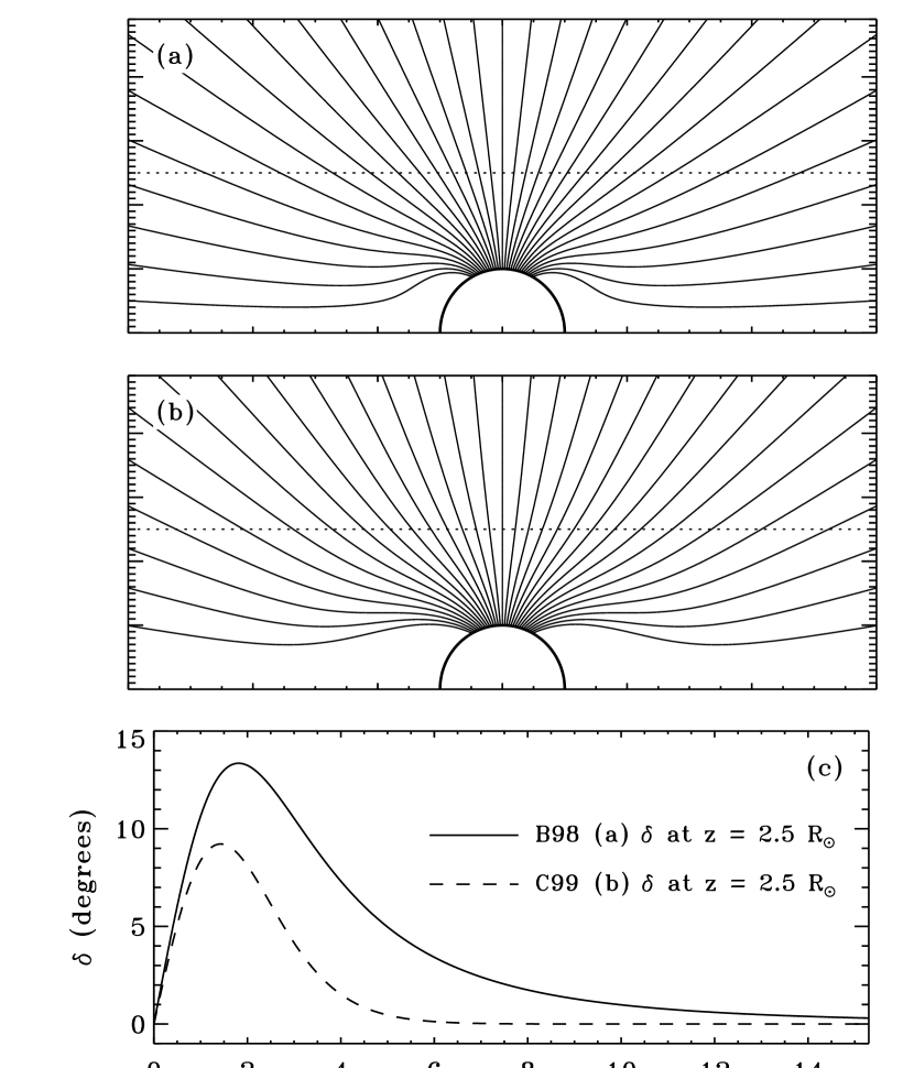
Figure 2.— Magnetic field lines in the plane of the sky for (a) the B98 (Banaszkiewicz et al.  1998) model, and (b) the C99 (Cranmer et al.  1999) model that used the Kopp & Holzer (1976) flux-tube area function. The dotted horizontal line denotes the position of the LOS along which various quantities are plotted in (c). In panel (c), the superradial angle $\delta$ is given as a function of $|x|$ (it is the same in the foreground and background halves of the LOS) for the two models shown above (see labels).

Figure 2 illustrates the differences between the magnetic geometries used in models R and C. Figures 2a and 2b show field lines that are distributed evenly in polar angle $\theta$ between 0° and 29° as measured on the solar surface from the north pole. The superradial angle $\delta$ characterizes the departure from the radial direction, and it is shown in Figure 2c as a function of LOS distance $x$ for a polar observing height $z=2.5\,R_{\odot}$. Formally, $\delta$ is defined as the angle between the radius vector ${\bf r}$ and the magnetic field ${\bf B}$ (assuming the field points outward), i.e.,

$$\delta\,=\,\cos^{-1}\left(\frac{{\bf r}\cdot{\bf B}}{|{\bf r}|\,|{\bf B}|}\right)\,\,.$$ (9)

For the polar observations described here, the LOS projection of any quantity that follows the magnetic field (e.g., the outflow velocity) is given by multiplying its magnitude by $\sin(\theta+\delta)$. The Banaszkiewicz et al.  (1998) model exhibits a larger degree of departure from radial geometry than does the Cranmer et al.  (1999) model. However, at the large heights for which the UVCS O VI anisotropy results are of interest here, the relative differences between the two models—and also the differences between either model and a radial geometry ($\delta=0$)—are small.

Figure 3 shows the range of electron densities measured by several instruments in polar coronal holes. The strong radial decrease in $n_{e}(r)$ has been removed by dividing all measurements by equation (8). The use of this normalization more clearly illustrates the relative differences between the different sets of values, which Raouafi & Solanki (2004, 2006) claimed to be important in the derivation of O⁵⁺ temperature anisotropy. The differences between plumes and interplume regions is certainly responsible for some of the wide range of variation, but some of it may also be due to absolute calibration uncertainties between instruments. Note, though, that the curve representing the hydrostatic equation (1) of Doyle et al.  (1999) appears to be clearly divergent from the other empirical curves above $r\approx 8\,R_{\odot}$, with a slope that is flatter than the other measurements even several solar radii below that.

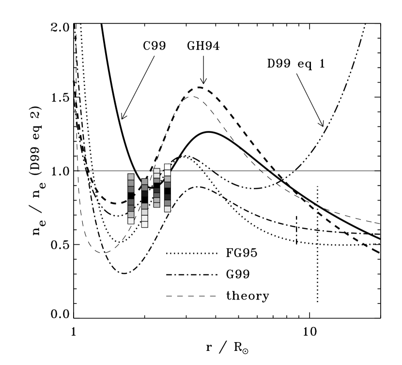
Figure 3.— Comparison of measured electron densities in polar coronal holes. Values of $n_{e}$ from Guhathakurta & Holzer (1994) (thick dashed line), Fisher & Guhathakurta (1995) (dotted line & vertical bar), Guhathakurta et al.  (1999) (dot-dashed line & vertical bar), and Cranmer et al.  (1999) (thick solid line) were divided by equation (8), i.e., equation (2) of Doyle et al.  (1999). The polar theoretical model of Cranmer et al.  (2007) is also shown (thin dashed line), as is the approximate hydrostatic fit from eq. (1) of Doyle et al.  (1999) (triple-dot-dashed line). Gray-scale histogram boxes show the range of $n_{e}$ values from the plume statistics study of Cranmer et al.  (1999), with darker shades denoting the most likely values at each height.

The gray-scale histogram boxes in Figure 3 illustrate the variations due to differing concentrations of polar plumes along a single polar LOS over three months (1996 November 1 to 1997 February 1) using a consistent data set and large enough count rates to make Poisson uncertainties negligible (see Table 3 of Cranmer et al.  1999). The curves from Fisher & Guhathakurta (1995) and Guhathakurta et al.  (1999) show averages of the various plume and interplume values given in those papers, with vertical lines illustrating the relative contrast between the densest plume-filled lines of sight and the regions with the fewest numbers of plumes. (These vertical lines are shown at $r\approx 10\,R_{\odot}$ for clarity, but they are representative of the values at the lower heights corresponding to the observed white-light data.) Polar electron density values reported recently by Quémerais et al. (2007) are not shown, but they are similar in radial shape to the Fisher & Guhathakurta (1995) mean curve (but with values about 10%–20% higher). Overall, the variations between data sets that appear to exceed the plume-interplume contrast may be due to different instrument calibrations.

When modeling the O VI observations summarized in § 2, it is probably incorrect to use the lowest “pure interplume” electron densities. At $z\approx 2.5$–3 $R_{\odot}$ in polar coronal holes, the UVCS observations were typically integrated over 15′ to 30′ in the tangential direction, whereas polar plumes at these heights have transverse sizes of only about 1′ to 2′. Thus, the most appropriate electron densities to use are those that average over plumes and interplume regions. The lower limits from Fisher & Guhathakurta (1995) and Guhathakurta et al.  (1999), as well as the fitting function given by Esser et al.  (1999), seem to be inappropriate to apply to the empirical modeling of these UVCS O VI data. At lower heights, where the plume and interplume regions have been resolved by UVCS (e.g., Kohl et al.  1997; Giordano et al.  2000), the use of the full range of plume and interplume values of $n_{e}$ would be warranted.

3.3. Comparison with Observations

Once a model data cube (which varies $u_{i\parallel}$, $T_{i\perp}$, and $T_{i\perp}/T_{i\parallel}$ along its axes) has been produced for a given observing height $z$ and a given set of $n_{e}$, $T_{e}$, and flux tube parameters, the next step is to compute the probability of agreement between a given observation and each of the simulated observations in the cube. We compute this probability $P$ as the product of two quantities that are assumed to be independent of one another: (1) the probability $P_{\rm R}$ that the observed line ratio agrees with the simulated ratio, and (2) the probability $P_{\rm S}$ that the observed profile shape of the O VI $\lambda$1032 line agrees with the simulated shape. Because the brighter O VI $\lambda$1032 line tends to dominate the measured “weighted” line width $V_{1/e}$, we use only the simulated O VI $\lambda$1032 line shape in the latter comparison.

The line ratio probability $P_{\rm R}$ is relatively straightforward to compute. The modeled total intensities of the two components of the doublet are determined by summing up the specific intensities over the 12 wavelength bins. Their ratio thus gives ${\cal R}_{\rm model}$. The relative distance between ${\cal R}_{\rm model}$ and the observed ratio ${\cal R}_{\rm obs}$, in units of the observational standard deviation ($\delta{\cal R}_{\rm obs}$), is the quantity that determines the probability of agreement. Assuming the uncertainties are normally distributed, the probability is

$$P_{\rm R}\,=\,1-\mbox{erf}\left(\frac{|{\cal R}_{\rm obs}-{\cal R}_{\rm model}|}{\delta{\cal R}_{\rm obs}\,\sqrt{2}}\right)$$ (10)

(see, e.g., Bevington & Robinson 2003). A larger argument in the error function (“erf” above) denotes a larger discrepancy between the modeled and observed ratios, and thus a lower probability of agreement.

The line shape probability $P_{\rm S}$ is not as easy to compute as $P_{\rm R}$. An initial attempt was made to fit the simulated profiles with Gaussian functions, and then to compare the resulting $V_{1/e}$ widths with the observed values using a similar expression as equation (10). However, there were many instances where the modeled lines were far from Gaussian in shape, but the best-fitting Gaussian (which was a poor fit in an absolute sense) happened to agree with the observed $V_{1/e}$. This resulted in spuriously high probabilities for wide regions of parameter space that should have been excluded. Thus, we found that the tabulated specific intensities (i.e., the full line shapes) need to be compared on a wavelength-by-wavelength basis. This raises the issue of what to use for the “observed” line shape. As described in § 2, the UVCS/SOHO data points contain a wide range of instrumental effects that were taken into account in the line fitting process. In order to compare similar quantities, either these effects must be inserted into the model profiles, or we must reconstruct “observed profile” information from the extracted $V_{1/e}$ measurements and the $\delta V_{1/e}$ uncertainties. We chose the latter option.

To determine the probability of agreement between the set of modeled specific intensities ($I_{\lambda,{\rm model}}$) and the reconstructed observed intensities ($I_{\lambda,{\rm obs}}$), we computed a $\chi^{2}$ quantity,

$$\chi^{2}\,=\,\sum_{\lambda}\left(\frac{I_{\lambda,{\rm obs}}-I_{\lambda,{\rm model}}}{\delta I_{\lambda,{\rm obs}}}\right)^{2}$$ (11)

where $I_{\lambda,{\rm model}}$ came from the data cube, and $I_{\lambda,{\rm obs}}$ was constrained to be a Gaussian function with the observed $V_{1/e}$ width and a total intensity equal to that of the modeled profile. (The observed total intensity was not used because the comparison being done here is only between the relative shapes.) The $\delta I_{\lambda,{\rm obs}}$ uncertainty was computed as a function of wavelength by comparing the idealized $I_{\lambda,{\rm obs}}$ profile with two others computed with line widths $V_{1/e}-\delta V_{1/e}$ and $V_{1/e}+\delta V_{1/e}$ (with all three profiles normalized to the same modeled total intensity). These three profiles exhibited a range of specific intensities at each wavelength, and the standard deviation quantity $\delta I_{\lambda,{\rm obs}}$ was defined as half of that full range. Then, the $\chi^{2}$ quantity above constrains the probability that the observed and modeled profiles are in agreement (i.e., the probability that the observed and modeled specific intensity values are drawn from the same distribution). Assuming normally distributed uncertainties, this probability is given by

$$P_{\rm S}\,\equiv\,Q(\chi^{2}|\nu)=\frac{1}{\Gamma(\nu/2)}\int_{\chi^{2}/2}^{\infty}e^{-t}t^{(\nu/2)-1}dt$$ (12)

(Press et al.  1992), where $\nu=N_{\lambda}-1$ is the effective number of degrees of freedom (for $N_{\lambda}=12$ wavelength points) and $\Gamma(x)$ is the complete Gamma function. When $\chi^{2}\ll\nu$ the above probability approaches unity (i.e., the modeled profile is a good match to the observed profile), and when $\chi^{2}\gg\nu$ the above probability is negligibly small.

We thus obtained the total probability $P=P_{\rm R}P_{\rm S}$ as a function of the three main O⁵⁺ variables of each data cube, for each observation at the height $z$ consistent with that data cube. The question of what is considered to be a large or small probability is open to some interpretation. Below, we often use a standard “one sigma” probability $P_{1\sigma}=1-\mbox{erf}(1/\sqrt{2})=0.317$ as a fiducial value above which the solutions are considered to be good matches with the data.

4. Empirical Model Results

In this section we present results for the most probable values of the O⁵⁺ ion properties between 1.5 and 3.5 $R_{\odot}$. In § 4.1, we show how the essential information inside the three-dimensional probability cubes can be extracted and analyzed in a manageable way. In § 4.2, the optimal values for O⁵⁺ outflow speed and perpendicular temperature are presented for models C and R. The resulting values of $u_{i\parallel}$ and $T_{i\perp}$ are consistent with earlier determinations of preferential ion heating and acceleration with respect to protons. In § 4.3, we discuss the determination of the anisotropy ratio $T_{i\perp}/T_{i\parallel}$ for models C and R, which is less certain than the other two quantities. We then focus in detail on a single representative height in § 4.4 in order to determine how models C and R can give rise to qualitatively different conclusions about the ion temperature anisotropy. Finally, in § 4.5 we extract information from both models C and R about the O⁵⁺ ion concentration in the extended corona—i.e., we compute the ratio $n_{{\rm O}^{5+}}/n_{\rm H}$ from the comparison of observed and modeled O VI $\lambda$1032 total intensities.

4.1. Deriving Ion Properties from the Data Cubes

We constructed two sets of radially dependent data cubes: one for the model C assumptions for $n_{e}$, $T_{e}$, and flux-tube geometry, and one for model R. Each set consisted of 13 data cubes with observation heights $z=1.5$, 1.6, 1.7, 1.8, 1.98, 2.11, 2.3, 2.42, 2.563, 2.7, 3.0, 3.09, and 3.565 $R_{\odot}$. These values were chosen to align with the observed data points shown in Figure 1. Any discrepancies between the observed and modeled heights never exceeded $\pm 0.065\,R_{\odot}$, and for the whole data set the average absolute value of the discrepancy was only 0.012 $R_{\odot}$. We then constructed 49 individual “probability cubes” for each of the data points for which both $V_{1/e}$ and ${\cal R}$ exist.

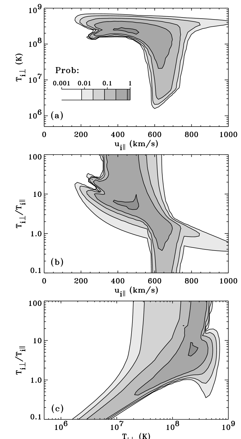
Figure 4.— Contour plots of the maximum probabilities of agreement between the model R data cube and the UVCS observation from 1997 January 5 at $r=3.07\,R_{\odot}$. The three panels show probabilities as a function of each unique pair of the three data-cube axis quantities. Contour levels are plotted at 90% of the probability values 1, 0.3, 0.1, 0.03, and 0.01 (see gray-scale code in panel a).

Even for just a single comparison between an observation and a data cube at one height, it is a challenge to display the full three-dimensional nature of the probability “cloud” $P(u_{i\parallel},T_{i\perp},T_{i\perp}/T_{i\parallel})$. We limit ourselves to showing lower-dimensional projections that keep only the highest probability values taken over the axes that are not being shown. As an example, in Figure 4 we display two-dimensional contours of $P$ as a function of all three unique pairings of the three axis-quantities of the data cube. The specific comparison is between the measurement shown in Table 1 from 1997 January 5 ($3.07\,R_{\odot}$, $V_{1/e}=690$ km s^-1) and the model R data cube constructed at $z=3.09\,R_{\odot}$. In all three contour plots, the probability shown at each location is a maximum taken over the third quantity that is orthogonal to the projection plane. Thus, for regions with a low probability in these diagrams, we can be assured that there are no values of the unplotted coordinate that can give synthetic line profiles in agreement with the observations.

Figure 4a shows an approximate anticorrelation between the ion outflow speed and the perpendicular kinetic temperature in the subset of generally “successful” models. This arises mainly because the lines can be broadened both by microscopic LOS motions (roughly proportional to $T_{i\perp}$) and by the projection of the superradially flowing bulk outflow speed along the LOS (which goes as $u_{i\parallel}$). When one of these quantities goes up, the other must go down in order to match a given observed line profile. Figure 4b shows that the region of parameter space with the larger contribution by $T_{i\perp}$ (upper left) also requires a large anisotropy ratio, but the region with the larger contribution by bulk LOS motions (lower right) may be able to match the observations with an isotropic velocity distribution (i.e., $T_{i\perp}/T_{i\parallel}\approx 1$).

The large amount of information in contour plots like Figure 4 can be collapsed down to a smaller list of parameters. We created three one-dimensional probability curves as a function of each of the three main axis quantities, with the maximum values extracted from the full plane subtended by the remaining two neglected quantities. Thus, we define the reduced probability functions $P_{u}(u_{i\parallel})$, $P_{t}(T_{i\perp})$, and $P_{a}(T_{i\perp}/T_{i\parallel})$ (the subscript “$a$” denotes the anisotropy ratio). These functions are generally peaked at some high value close to 1 and exhibit lower values far from the optimal solutions. Figure 5 shows these reduced probabilities for the same example case shown in Figure 4. The reduced probabilities for $u_{i\parallel}$ and $T_{i\perp}$ are peaked relatively sharply around their most probable values. Note that we plot the perpendicular kinetic temperature in units of a most-probable speed $w_{i\perp}=(2k_{\rm B}T_{i\perp}/m_{i})^{1/2}$ in order to facilitate comparison with earlier papers. The reduced probability for the anisotropy ratio, shown in Figure 5b, is less centrally peaked and thus the best solution for this value is less certain. The peak value corresponds to a most-probable anisotropy ratio of $T_{i\perp}/T_{i\parallel}\approx 6$, but note that the probability of isotropy remains reasonably high at $\sim$40%.

Figure 5.— Reduced probabilities for one specific comparison between a UVCS observation at $r=3.07\,R_{\odot}$ and the model R data cube (see also Figs.  4, 8, 10, and 11). (a) $P_{u}$ versus outflow speed $u_{i\parallel}$ (solid line) and $P_{t}$ versus perpendicular most-probable speed $w_{i\perp}$ (dashed line). (b) $P_{a}$ versus anisotropy ratio $T_{i\perp}/T_{i\parallel}$ for a search of the entire data cube (solid line) and for a “slice” through the data cube with fixed values of $u_{i\parallel}$ and $w_{i\perp}$ given above (dashed line). Also shown is the threshold level $P_{1\sigma}$ (dotted lines) defined in the text.

It is interesting to contrast the exhaustive data-cube-search technique used here with the more straightforward approaches taken in earlier papers. For example, Raouafi & Solanki (2004, 2006) simulated the properties of the O VI $\lambda\lambda$1032, 1037 lines after first fixing the radial variation of the outflow speed and ion temperature. Figure 5b shows an illustrative “cut” through the data cube at fixed values of $u_{i\parallel}=600$ km s^-1 and $w_{i\perp}=215$ km s^-1 at $r=3.09\,R_{\odot}$ (similar to the values used by Raouafi & Solanki 2006). In this case, the most probable value of the anisotropy ratio is surprisingly close to 1, as was also assumed by Raouafi & Solanki. The apparent consistency with the observations (i.e., a value of $P_{a}$ of about 30%) may be misleading if the rest of the data cube is not searched. Thus, we can assert that any results concerning the anisotropy ratio that were obtained by not searching the full range of possibilities for the ion parameters are potentially inaccurate.

The ultimate goal of the empirical modeling process is to characterize the peak values and widths of the reduced probability curves, in order to obtain the optimal measured values (with uncertainty limits) for the relevant O⁵⁺ plasma properties. The most satisfactory outcome, of course, would be very narrow peaks that occur far from the edges of the parameter space, but this is not always the case. After some experimentation, we chose to use weighted means to obtain the peak values, i.e.,

$$\langle x\rangle\,=\,\frac{\int dx\,x\,P_{x}(x)}{\int dx\,P_{x}(x)}$$ (13)

where $x$ denotes any of the three axis quantities $u_{i\parallel}$, $T_{i\perp}$, or $\log(T_{i\perp}/T_{i\parallel})$. We used the logarithm of the anisotropy ratio in equation (13) because tests showed that if the ratio itself (which spans three orders of magnitude) was used, the above mean would be weighted strongly toward the largest values even when the maximum of the probability distribution is at much lower values.

We experimented with using the variance, or second moment, of the reduced probability distributions to characterize the widths of “error bars” for each measurement. However, because the probability curves are generally not symmetric around the peak values, the second moment often did not accurately give a range of values with reasonable probabilities. Instead, we performed a straightforward search for the range of probabilities that are higher than the threshold value $P_{1\sigma}\approx 0.317$ discussed above. The lower and upper limits of that range were taken to be the ends of the uncertainty bounds for each measurement.

4.2. Preferential Ion Heating and Acceleration

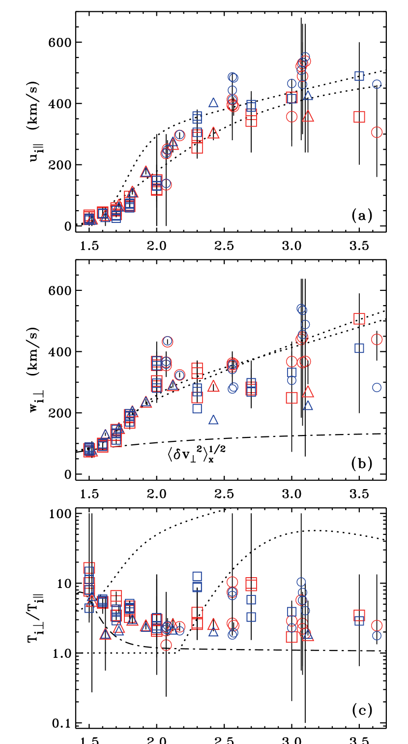
Figure 6.— Derived outflow speeds (a), perpendicular most-probable speeds (b), and kinetic anisotropy ratios (c) for model R (red points) and model C (blue points). Symbols show the weighted means of the reduced probability distributions, with styles the same as in Figure 1. Vertical bars show the full range of parameter space with reduced probabilities greater than $P_{1\sigma}$ (for model R). Also shown are empirical models B1 and B2 from Cranmer et al.  (1999) (dotted lines) and Alfvén wave quantities $\langle\delta v_{\perp}^{2}\rangle_{x}^{1/2}$ in panel (b) and $A_{\rm eff}$ in panel (c), derived from the model of Cranmer et al.  (2007) (dot-dashed lines).

Figure 6 shows the weighted mean and error-bar quantities for the O⁵⁺ plasma properties, defined as in the previous subsection, as a function of heliocentric height. The results from model C and model R are plotted in two different colors, with only the error bars of model R shown for clarity. Here we focus on the ion outflow speed (Fig.  6a) and the perpendicular ion temperature (Fig.  6b). On average, the derived values of $\langle u_{i\parallel}\rangle$ and $\langle w_{i\perp}\rangle$ were consistent between the two sets of models. To quantify the impact of varying the electron density, electron temperature, and flux-tube geometry, we computed ratios of the model C values to the model R values for each data point. For the 49 data points taken together, the mean value of the ratio of the outflow speeds was 1.002, with a standard deviation of 19%, and the mean value of the ratio of perpendicular most-probable speeds was 0.991, with a standard deviation of 14%. This shows that the determination of these parameters is relatively insensitive to the choices of electron density, electron temperature, and flux-tube geometry.

The radial dependence of the derived $\langle u_{i\parallel}\rangle$ values in Figure 6a is similar to that of the O⁵⁺ empirical models B1 and B2 given by Cranmer et al.  (1999). Note the emergence of a natural trend of radial acceleration in $\langle u_{i\parallel}\rangle$, with the possible exception of the data points at $r\gtrsim 3.5\,R_{\odot}$. This is especially serendipitous given that each data point was analyzed independently of all others.

The derived O⁵⁺ outflow speeds support earlier claims of preferential ion acceleration in coronal holes. At $r=2.5\,R_{\odot}$, the range of ion outflow speeds that gives rise to high probabilities of agreement with the data points is approximately 280–500 km s^-1 At this height, these values are substantially larger than bulk (proton-electron) solar wind outflow speeds derived via mass flux conservation. Figure 41 of Kohl et al.  (2006) showed a selection of 12 bulk outflow speed models derived using all possible combinations of four $n_{e}$ models and three coronal-hole geometries. At $r=2.5\,R_{\odot}$, these 12 models gave a range of bulk outflow speeds of 115–300 km s^-1. Despite the small degree of overlap between the two ranges, the mean value of the O⁵⁺ range (390 km s^-1) exceeds the mean value of the mass flux conservation range (208 km s^-1) by almost a factor of two. Also, proton outflow speeds derived from H I Ly$\alpha$ Doppler dimming (from a selection of papers all dealing with polar coronal holes at the 1996–1997 solar minimum) were shown in Figure 41 of Kohl et al.  (2006). At 2.5 $R_{\odot}$, the range of these values is 160–260 km s^-1—with a mean of 210 km s^-1—which is still significantly lower than the range of O⁵⁺ ion outflow speeds discussed above.

In Figure 6b, the trend of radial increase in $\langle w_{i\perp}\rangle$ is also roughly similar to that found by Cranmer et al.  (1999), especially below about 2.3 $R_{\odot}$. At larger heights, though, there appears to be less evidence for a systematic increase than existed in the model B1 and B2 curves. This could have resulted either from the inclusion of the new data points or from the more exhaustive treatment of uncertainties in the new parameter determination method described above. However, if one takes all of the derived $\langle w_{i\perp}\rangle$ values for $r\geq 2\,R_{\odot}$ and fits to a straight line, the best-fitting slope is still increasing with height at a rate of 50 km s^-1 per $R_{\odot}$. This is about a third of the $\sim$150 km s^-1 per $R_{\odot}$ slope in the B1 and B2 models.

The most-probable speeds $\langle w_{i\perp}\rangle$ shown in Figure 6b, although slightly smaller than those given by the Cranmer et al.  (1999) model B1 and B2 curves at some heights, still show definite evidence for preferential ion heating. The mean value of the $\langle w_{i\perp}\rangle$ values at heights $r\geq 2.5\,R_{\odot}$ in Figure 6b is 363 km s^-1, with a standard deviation of 73 km s^-1. Between 2.5 and 3 $R_{\odot}$, the perpendicular proton most-probable speeds derived from H I Ly$\alpha$ were about 210–240 km s^-1, with a mean value of about 225 km s^-1 (see models A1 and A2 of Cranmer et al.  1999). The fact that the O⁵⁺ mean value exceeds the proton mean value by almost two standard deviations implies that the O⁵⁺ kinetic temperature at this height is very likely to be more than “mass proportional” (i.e., implying an oxygen kinetic temperature of 130 MK, or more than 40 times the proton kinetic temperature of $\sim$3 MK.

It is important to note that the derived kinetic temperatures are likely to be a combination of thermal and nonthermal motions. The ion-to-proton kinetic temperature ratio of $\sim$40, derived above, is likely to be a lower limit to the true ratio of thermal, or microscopic temperatures. If unresolved wave motions are deconvolved from the empirical values of $\langle w_{i\perp}\rangle$, the proton most-probable speed will be reduced by a relatively larger amount than the O⁵⁺ speed. As an example, the theoretical polar coronal hole model of Cranmer et al.  (2007) has a LOS-projected Alfvén wave amplitude at $r=2.5\,R_{\odot}$ of 116 km s^-1 (this is also plotted in Fig.  6b). Converting these motions into temperature-like units and subtracting from both values given above, one obtains an O⁵⁺ perpendicular temperature of 115 MK and a proton perpendicular temperature of 2.2 MK. The ratio of ion to proton temperatures has thus increased from about 40 to 50. In any case, it is clear that the dominant contributor to the ion kinetic temperature is the true “thermal” temperature, with only a relatively minor impact from broadening due to macroscopic motions.

4.3. The Ion Anisotropy Ratio

Figure 6c illustrates the largest discrepancy between the empirical models of Cranmer et al.  (1999) and the present models (both C and R). Above a height of $\sim$2.5 $R_{\odot}$, models B1 and B2 demanded a strong anisotropy ratio $T_{i\perp}/T_{i\parallel}>10$, but the optimal ratios derived in this paper seem to cluster between 2 and 10 with no discernible radial dependence. It is important to note, though, that there is considerable overlap of the uncertainties between the old and new ranges of $\langle T_{i\perp}/T_{i\parallel}\rangle$. Several of the error bars shown in Figure 6c extend up into the range of ratios from models B1 and B2. Also, the dotted curves that illustrate models B1 and B2 correspond to the “optimal” values of the anisotropy ratio from Kohl et al.  (1998) and Cranmer et al.  (1999); the uncertainties in those models are not shown.

Because the derived values of the kinetic temperature ratio $\langle T_{i\perp}/T_{i\parallel}\rangle$ in Figure 6c exceed unity by only a relatively small amount, it is worthwhile to examine whether the numerator ($T_{i\perp}$) may have been enhanced by unresolved wave motions perpendicular to the magnetic field. In other words, for a realistic model of perpendicular wave amplitudes in polar coronal holes, we investigate whether a truly isotropic microscopic velocity distribution could have given an effective anisotropy ratio that exceeds 1. We compute such an effective anisotropy ratio as

$$A_{\rm eff}\,=\,\frac{1}{1-(\langle\delta v_{\perp}^{2}\rangle_{x}/w_{i\perp}^{2})}\,\,,$$ (14)

where $\langle\delta v_{\perp}^{2}\rangle_{x}$ is the square of the frequency-integrated Alfvén wave amplitude divided by two to sample only the motions along one of the two perpendicular directions (i.e., only along the LOS or $x$ axis). As above, we used the Alfvén wave properties from the turbulence-driven polar coronal hole model of Cranmer et al.  (2007). The model wave amplitude is plotted in Figure 6b and the quantity $A_{\rm eff}$ is plotted in Figure 6c. The condition $A_{\rm eff}\approx 1$ corresponds to the situation where the amplitudes are too small to contribute to the anisotropy ratio (as defined in the empirical models). Below $r\approx 1.7\,R_{\odot}$, the curve in Figure 6c shows that $A_{\rm eff}$ does indeed exceed 1 by about the amount computed from the UVCS data. At these low heights, the derived value of $\langle w_{i\perp}\rangle$ is of the same order of magnitude as the wave amplitude, so the latter can “contaminate” the determination of the true perpendicular most-probable speed. At heights larger than about 2 $R_{\odot}$, though, the wave amplitudes are small in comparison to the derived $\langle w_{i\perp}\rangle$ values, and thus $A_{\rm eff}\approx 1$. We thus conclude that above 2 $R_{\odot}$, any derived anisotropy ratio $\langle T_{i\perp}/T_{i\parallel}\rangle$ is likely to be truly representative of the microscopic velocity distribution and not affected by wave motions.

Despite the comparatively low values of the anisotropy ratio shown in Figure 6c ($\langle T_{i\perp}/T_{i\parallel}\rangle\approx 2$–10), we should emphasize that these values are often significantly different from unity. It is important to note that all of the data points have their largest reduced probability—measured either using the weighted mean defined above or by simply locating the maximum value—for anisotropy ratios larger than unity.

Figure 7.— Probability of ion isotropy $P_{a}(1)$ plotted versus heliocentric distance for model R, using the same data symbols as Figures 1 and 6. The filled circle shows the probability of isotropy for the specific observation ($3.07\,R_{\odot}$, $V_{1/e}=690$ km s^-1) that is considered in detail in Figures 4, 5, 8, 10, and 11.

The preponderance of evidence for anisotropy is also illustrated in Figure 7, which shows the probability that each measurement could be explained by an isotropic O⁵⁺ velocity distribution. In other words, Figure 7 gives the value of $P_{a}(1)$ for each probability cube. Taken together, a significant majority of the values (about 78% of the total number) fall below the fiducial one-sigma value of $P_{1\sigma}$, indicating that isotropy should not be considered a “baseline” assumption. Below about $r=2\,R_{\odot}$, a few of the measurements correspond to large probabilities that an isotropic distribution can explain the observations. Note from Figure 6c, though, that the most-probable anisotropy ratios for these measurements tend to be greater than 1, but some of the error bars extend down past $T_{i\perp}/T_{i\parallel}=1$. However, between 2.1 and 2.7 $R_{\odot}$ the probability of isotropy is very small for all of the observed data points. Above 3 $R_{\odot}$, some of the values of $P_{a}(1)$ become large again, but we believe this may be due to the relatively high observational uncertainties on the O VI intensities and line widths at these large heights (see below).

Figure 8.— Reduced probability $P_{a}$ versus ion anisotropy ratio $T_{i\perp}/T_{i\parallel}$ for one specific comparison between a UVCS observation at $r=3.07\,R_{\odot}$ and the model R data cube (see also Figs.  4, 10, and 11). The probability computed with the actual observational uncertainties (thick solid line) is compared with trial curves computed with a range of constant factors $\epsilon$ multiplying $\delta V_{1/e}$ and $\delta{\cal R}$ (dashed lines). Also shown is the threshold level $P_{1\sigma}$ (dotted line) and the probability of isotropy for the standard $\epsilon=1$ case that is also shown in Figure 7 (filled circle).

To better understand the impact of observational uncertainties on the probability of isotropy, Figure 8 shows the full $P_{a}(T_{i\perp}/T_{i\parallel})$ curves for one specific measurement at $r=3.07\,R_{\odot}$ (i.e., the same measurement used in Fig.  5). The multiple curves were constructed by multiplying the known observational uncertainties $\delta V_{1/e}$ and $\delta{\cal R}$ by arbitrary factors $\epsilon$. Generally, larger uncertainties lead to lower $\chi^{2}$ values when comparing the observed and modeled line shapes, and thus to larger probabilities of agreement between the observed and modeled profiles. Interestingly, though, the anisotropy ratio $T_{i\perp}/T_{i\parallel}$ at which the maximum probability occurs remains roughly constant when $\epsilon$ is varied between 0.5 and 2. Thus, if future observations above 3 $R_{\odot}$ were to obtain the same general range of values for $V_{1/e}$ and ${\cal R}$ but with lower uncertainties, it could provide stronger evidence for ion anisotropy up at these heights.

Although Figure 6c does not seem to indicate a substantial difference between models R and C, it is useful to compare these models in some additional detail. For all data points, the mean ratio of model C to model R anisotropy ratios was 1.199, but the large standard deviation (76%) shows that the models are often quite different from one another. Taking only the heights above 2.2 $R_{\odot}$, the mean ratio of model C to model R anisotropy ratios increases to 1.514, indicating that on average model C generates larger anisotropies than model R over the height range where anisotropies appear to be required.

Figure 9.— Ratios of model C to model R values for the weighted mean anisotropy ratios $\langle T_{i\perp}/T_{i\parallel}\rangle$ shown as a function of height and using the same data symbols as Figures 1, 6, and 7.

Figure 9 shows the ratio of model C to model R anisotropy ratios as a function of height. Below $r\approx 2.2\,R_{\odot}$ the two models produce roughly the same result for the anisotropy ratio. Above that height, the solutions split into two groups: one where model C produces a substantially larger ratio (2–3 times that of model R), and one where model C produces a comparable or slightly smaller ratio than model R. Note that the height range of 3.0–3.1 $R_{\odot}$—over which model R predicted a rise in the probability of isotropy (see Fig.  7)—strongly favors larger anisotropies for model C.

4.4. Varying the Electron Density, Electron Temperature, and Geometry

One of the main motivations for this paper was to explore why the results of Raouafi & Solanki (2004, 2006) were so different from earlier results (e.g., Cranmer et al.  1999) regarding the O⁵⁺ anisotropy ratio. In this subsection, we study the differences between model R and model C in more detail by focusing on the shapes of the reduced probability distributions for one representative data point. As in Figures 4, 5, and 8, we used the probabilities generated by comparing the UVCS/SOHO measurement from 1997 January 5 ($r=3.07\,R_{\odot}$, $V_{1/e}=690$ km s^-1) with data cubes constructed with various assumptions. This data point is denoted by a filled circle in Figure 9, and it is clear that this point is representative of the majority of the data points (5 out of 7) at $r\approx 3\,R_{\odot}$.

Figure 10 shows a range of reduced probability curves $P_{a}(T_{i\perp}/T_{i\parallel})$ that were computed from data cubes constructed with various combinations of the model R and model C parameters. The three-letter names for the models denote the individual choices for $n_{e}$, flux-tube geometry, and $T_{e}$ (in that order). The “pure” model R and model C cases are thus called RRR and CCC.

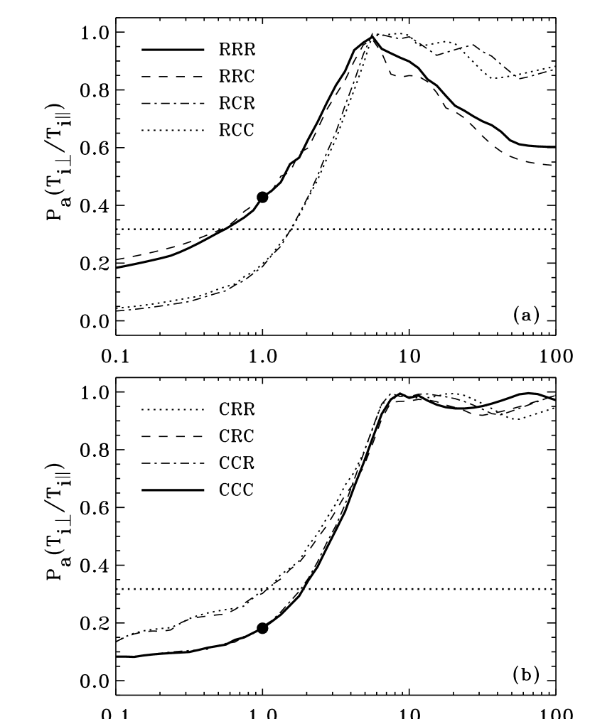
Figure 10.— Reduced probability $P_{a}$ versus ion anisotropy ratio $T_{i\perp}/T_{i\parallel}$ for the same data comparison as in Figures 4 and 8, but for various combinations of the model R and model C parameters (see above for line styles). The order of the three-letter designations is $\{n_{e},f(r),T_{e}\}$. Panel (a) thus shows all models computed with the Doyle et al.  (1999) $n_{e}$ and panel (b) shows all models computed with the Cranmer et al.  (1999) $n_{e}$. Also shown is the threshold level $P_{1\sigma}$ (horizontal dotted lines) and the probability of isotropy for the main RRR and CCC cases (filled circles).

Before examining the impact of the individual parameters on the reduced probability curves, we note that the model CCC curve in Figure 10b mirrors almost exactly the results of Kohl et al.  (1998) and Cranmer et al.  (1999) at $r\approx 3\,R_{\odot}$: the most likely O⁵⁺ anisotropy ratio ranges between 10 and 100, and an isotropic distribution is highly improbable. Model CCC exhibits a most probable ion outflow speed $\langle u_{i\parallel}\rangle=508$ km s^-1, which is only marginally smaller than the model RRR value of 521 km s^-1. Model CCC has an optimal solution for $\langle w_{i\perp}\rangle$, though, of 541 km s^-1, which is 23% larger than the corresponding value of 440 km s^-1 for model RRR (i.e., a 51% higher value of $\langle T_{i\perp}\rangle$ for model CCC). Model CCC tended to produce more line broadening via “thermal” motions near the plane of the sky, and model RRR tended to produce more line broadening via bulk outflow projected along the LOS.

The other curves shown in Figure 10 explore which of the three varied parameters were most responsible for the differences between models RRR and CCC. We see immediately that the choice of electron temperature $T_{e}$, which in our models impacts only the collision rate $q_{12}$, is relatively unimportant. The 8 curves can thus be separated into 4 pairs, each of which has the same choice for $n_{e}$ and flux-tube geometry (i.e., RRX, RCX, CRX, and CCX, where ‘X’ denotes either option for $T_{e}$). The overall insensitivity to electron temperature is evident from the fact that the two curves in each pair are virtually indistinguishable from one another.

Figure 10 shows that the unique features of the RRX models (i.e., a higher probability of isotropy and a strong peak at $T_{i\perp}/T_{i\parallel}<10$) are only present when both the electron density and flux-tube geometry are treated using model R. The models with only one of these two parameters treated using model R (i.e., RCX and CRX) appear more similar to the CCX models. At large values of the anisotropy ratio, both the RCX and CRX models are virtually identical to the CCX models. At low values of the anisotropy ratio, the CRX model is roughly intermediate between the CCX and RRX models. Generally, though, the combination of the model R assumptions for electron density (e.g., Doyle et al.  1999) and flux-tube geometry (e.g., Banaszkiewicz et al.  1998) are needed to produce broad enough profiles via outflow speed projection along the LOS to explain the observations without the need for extreme temperature anisotropies. Specifically, this enhanced LOS projection effect arises for two coupled reasons.

1. As seen in Figure 2c, the Banaszkiewicz et al.  (1998) flux tubes are tilted to a greater degree away from the radial direction than the Cranmer et al.  (1999) flux tubes. Because of these larger values of $\delta$, a larger fraction of the outflow speed $u_{i\parallel}$ is projected into the LOS direction (when $|x|>0$) for model R.

2. Figure 3 shows that the Doyle et al.  (1999) electron density does not drop as rapidly with increasing height (between about 3 and 10 $R_{\odot}$) as nearly all of the other plotted $n_{e}$ functions. Thus, for observation heights at about 3 $R_{\odot}$, the Doyle et al.  (model R) electron density provides a relative enhancement for points along the foreground and background ($|x|>0$) in comparison to the plane of the sky ($x=0$).

Note also from Figure 3 that the electron density used for model C is about 10% to 30% larger than that used for model R at the heights of interest ($r\approx 3$–4 $R_{\odot}$). A higher value of $n_{e}$ is expected to result in emission lines that are dominated more by the collisional component of the emissivity, which scales as $n_{e}^{2}$ (eq. [2]), with a correspondingly weaker contribution from the radiative component, which scales linearly with $n_{e}$ (eq. [3]). Because of the different density dependences, the collisional component is not extended as far along the LOS as the radiative component. Thus, models with higher densities would be expected to behave more like model C (with emission dominated by the plane of the sky), and models with lower densities would be expected to behave more like model R (with emission extended over a larger swath of the LOS).

To explore the effects of varying the electron density, we repeated the model R data cube analysis (for the fiducial height shown in Figs.  8 and 10) with $n_{e}(r)$ multiplied by constant factors. Figure 11 shows the resulting reduced probability curves as a function of the O⁵⁺ temperature anisotropy. A model with half of the Doyle et al.  (1999) electron density has a lower preferred value of $T_{i\perp}/T_{i\parallel}$ and a much higher probability of isotropy than the standard model R. A model with double the Doyle et al.  (1999) electron density resembles model C in that there is a high preferred range of $T_{i\perp}/T_{i\parallel}$ and a low probability of isotropy. Despite the large change in appearance of the $P_{a}$ curves as shown in Figure 11, the preferred values of the outflow speed and perpendicular kinetic temperature do not vary by very much as $n_{e}$ is varied up and down by a factor of two: $\langle u_{i\parallel}\rangle$ changes by only about $\pm 8$% (increasing as $n_{e}$ decreases), and $\langle w_{i\perp}\rangle$ changes by only about $\pm 10$% (increasing as $n_{e}$ increases). These determinations appear to be relatively insensitive to the choices for $n_{e}$ and flux-tube geometry.

Figure 11.— Reduced probability $P_{a}$ versus ion anisotropy ratio $T_{i\perp}/T_{i\parallel}$ for the same data comparison as in Figures 4, 5, 8, and 10, but for a range of constant multipliers to the Doyle et al.  (1999) electron density. The basic “model R” $n_{e}$ (solid line) is compared to a model with half (dashed line) and double (dot-dashed line) this electron density function. Also shown is the threshold level $P_{1\sigma}$ (dotted line) and the probabilities of isotropy for the three curves (filled and open circles).

The ratio of collisional emissivity to the total line emission changes dramatically for the models shown in Figure 11. For model RRR, the optimal model in the data cube exhibited a collisional fraction of 93.7% for the O VI $\lambda$1032 line and a fraction of 44.6% for the O VI $\lambda$1037 line (the latter being “Doppler pumped”). The model with half of the model R density had lower collisional fractions for the $\lambda\lambda$1032, 1037 lines of 88.2% and 28.7%, respectively. The model with double the model R density had higher collisional fractions of 96.8% and 61.7%.

It is important to note, however, that the differences in collisionality for the models shown in Figure 10 are not as drastic as those shown in Figure 11. Model CCC exhibited collisional fractions for the $\lambda\lambda$1032, 1037 lines of 90.7% and 47.0%. These values are only a few percentage points different from the model RRR fractions. The other intermediate models have values that cluster between those of models RRR and CCC. The larger value of $n_{e}$ in the plane of the sky for model C is compensated—to some degree—by the slower decrease in $n_{e}$ along the LOS for model R. Thus, despite the superficial resemblance between the model CCC curve in Figure 10 and the “double $n_{e}$” curve in Figure 11, one cannot invoke a varying amount of collisionality to explain the differences between models R and C. The LOS extension effects discussed above are more subtle than simply varying $n_{e}$ by a constant amount.

Another way we explored the dependence of the reduced probabilities on electron density was to produce a set of three other models with alternate functional forms for $n_{e}(r)$, but the same flux-tube geometry and $T_{e}$ as used in model R. These models utilized the mean electron density curves from Guhathakurta & Holzer (1994), Fisher & Guhathakurta (1995), and Guhathakurta et al.  (1999) (see also Fig.  3), and the O VI data cubes were created only at the fiducial height of 3.09 $R_{\odot}$. The reduced probabilities $P_{a}$ for these models all fell within the general range of variation illustrated in Figure 10 and are not plotted. However, the construction of these models increased the number of data cubes with “model R-like” flux-tube and $T_{e}$ parameters to seven: i.e., these three new ones, the three models shown in Figure 11, and model CRR (with a model C electron density). We performed a regression analysis on the seven values of the probability of isotropy $P_{a}(1)$ and the weighted mean anisotropy $\langle T_{i\perp}/T_{i\parallel}\rangle$ to find the optimal functional dependence on two “independent” variables that characterize the electron density:

$$n_{3}\,\equiv\,\frac{n_{e}(3\,R_{\odot})}{10^{6}\,\mbox{cm}^{-3}}\,\,,\,\,\,\,\,\,\,n_{6}\,\equiv\,\frac{n_{e}(6\,R_{\odot})}{10^{6}\,\mbox{cm}^{-3}}$$ (15)

where the arbitrary normalizations serve only to keep the combined quantities (discussed below) of order unity. The quantity $n_{3}$ characterizes the electron density in the plane of the sky of the observation, and the ratio $n_{3}/n_{6}$ characterizes the large-scale density gradient and thus the relative enhancement of foreground and background regions along the LOS. From the discussion above, we expect that larger values of both $n_{3}$ and $n_{3}/n_{6}$ should result in lower probabilities of isotropy and higher most-probable values of the anisotropy ratio. Indeed, the regression analysis found that the modeled values of these quantities exhibited the lowest combined $\chi^{2}$ spread for a single independent variable that scales as $n_{3}^{1.83}/n_{6}$ (close to the product of $n_{3}$ and $n_{3}/n_{6}$). Figure 12 shows these values as well as the best-fitting quadratic functions to $P_{a}(1)$ and $\langle T_{i\perp}/T_{i\parallel}\rangle$. The combined dependence on both $n_{e}$ and its radial gradient appears to be a key factor in determining the relative probabilities of isotropy and strong anisotropy.

Figure 12.— Reduced probabilities of isotropy (diamonds) and weighted mean anisotropy ratios (triangles) for models having a range of $n_{e}$ values and identical flux-tube and $T_{e}$ properties (see text for details). All data-cube comparisons were computed for the same fiducial data point illustrated in Figures 4, 5, 8, 10, and 11. Curves denote the best fitting quadratic relations as a function of the optimized density quantity $n_{3}^{1.83}/n_{6}$.

Finally, we must evaluate which sets of choices for the electron density and the flux-tube geometry are most consistent with observed polar coronal holes. Figure 3 does seem to indicate that most measured $n_{e}$ curves (as well as one example theoretical result for $n_{e}$) behave more like the “model C” (Cranmer et al.  1999) case than the “model R” (Doyle et al.  1999) case. Between the heights of about 3 and 10 $R_{\odot}$, the majority of the curves in Figure 3 exhibit a steeper radial decrease than the Doyle et al.  (1999) model. Thus, the CCX or CRX models shown in Figure 10b appear to be more consistent with observations than the RRX or RCX models in Figure 10a. This then implies that substantial O⁵⁺ anisotropy ($T_{i\perp}/T_{i\parallel}\gtrsim 10$) is also preferred at large heights. The optimal choice of the flux-tube geometry is less certain. Ideally, observations of the nonradial shapes of polar plumes should be able to constrain the magnetic field geometry (see, e.g., Wang et al.  2007; Pasachoff et al.  2007), but it is unclear whether existing plume observations would be able to distinguish the subtle differences between, e.g., Figures 2a and 2b. In any case, the geometry does not seem to be as major an issue as the electron density, since the variance between the four curves in Figure 10b is not large.

4.5. Oxygen Ion Number Density

By comparing the observed and modeled total intensities of the O VI $\lambda$1032 line, it is possible to derive firm limits on the combined elemental abundance and ionization fraction of O⁵⁺. The ion concentration is useful both as a tracer of fast and slow solar wind streams (e.g., Zurbuchen et al.  2002) and as a possible diagnostic of the amount of preferential heating deposited in coronal holes (Lie-Svendsen & Esser 2005). A first attempt at determining the O⁵⁺ number density from UVCS data was made by Cranmer et al.  (1999), but the “data cube search” technique developed in this paper allows a much more definitive set of measurements to be made.

The numerical code that computes the O VI line emission used an arbitrary constant value for the ratio $f_{0}=n_{{\rm O}^{5+}}/n_{e}$ of $4.959\times 10^{-6}$, which was derived from the oxygen abundance of Anders & Grevesse (1989) and the measured O⁵⁺ ionization fraction of Wimmer-Schweingruber et al.  (1998). This is merely a fiducial value that does not affect the final determination of this ratio for a given UVCS observation. When comparing the results from an empirical model data cube with a specific observation, the probability values $P(u_{i\parallel},T_{i\perp},T_{i\perp}/T_{i\parallel})$ are used to construct a weighted mean of the modeled O VI $\lambda$1032 total intensity using equation (13), as well as lower and upper limits using the full range of models with probabilities that exceed $P_{1\sigma}$. These values are converted into “observed” ion concentration ratios $f_{\rm obs}$ by assuming that the ratio $f_{\rm obs}/f_{0}$ is equal to the ratio of the observed to the modeled values of $I_{\rm tot}$. By using the modeled weighted mean, lower limit, and upper limit of $I_{\rm tot}$ we obtain the weighted mean, upper limit, and lower limit of $f_{\rm obs}$. (Note that the lower limit of $I_{\rm tot}$ gives the upper limit of $f_{\rm obs}$ and vice versa.) Finally, $f_{\rm obs}$ is converted into the ratio of O⁵⁺ to total hydrogen number density ($n_{{\rm O}^{5+}}/n_{\rm H}$) by multiplying by a factor of 1.1 (assuming a helium to hydrogen number density ratio of 5%).

Figure 13 shows the resulting ion concentration ratios as a function of height for the full range of model C data points. There is a hint of systematic radial increase at low heights. A similar radial increase would be predicted for ions that flow substantially faster than protons in the corona (by a factor of two) and then flow only $\sim$10% faster than protons at 1 AU. Above 2 $R_{\odot}$, though, Figure 13 does not show any definitive radial trend. Taking account of the uncertainty limits, the data appear consistent with the O⁵⁺ ionization fraction being more or less “frozen in” (see, e.g., Hundhausen et al.  1968; Owocki et al.  1983; Ko et al.  1997). A linear least squares fit (using the logarithm of $n_{{\rm O}^{5+}}/n_{\rm H}$ as the ordinate) is also shown, but the relatively high uncertainties at large heights preclude any reliable interpretation of the slope.

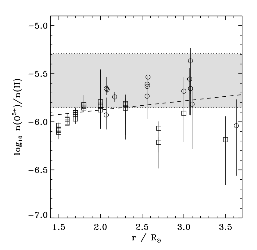
Figure 13.— O⁵⁺ ion number density ratio (with respect to hydrogen) as a function of heliocentric distance for model C. Symbols show the weighted means of the reduced probability distributions, with styles the same as in Figure 1. Vertical bars show the full range of parameter space with reduced probabilities greater than $P_{1\sigma}$. Also shown is a linear least-squares fit to the data points (dashed line) and empirical lower and upper limits as described in the text (gray region bounded by dotted lines).

Figure 13 also shows a range of values that would have been expected from prior studies of both the oxygen abundance and the O⁵⁺ ionization fraction. The abundance ratio ($n_{\rm O}/n_{\rm H}$) ranges from a relatively recent historical high of $8.5\times 10^{-4}$ (Anders & Grevesse 1989) to the more recent—and somewhat controversial—low of $4.6\times 10^{-4}$ (Asplund et al.  2004, 2005; Grevesse et al.  2007). The ionization fraction ($n_{\rm O^{5+}}/n_{\rm O}$) was measured in situ by the SWICS instrument on Ulysses (Wimmer-Schweingruber et al.  1998) to be about 0.0058 in the fast solar wind. Models that include the freezing in of heavy ions have produced values for this ratio from 0.0035 (Esser & Leer 1990) to about 0.005 (Chen et al.  2003). Although collisional ionization equilibrium is not expected to hold in the extended corona (for polar coronal holes), it is interesting to note that for $T_{e}=10^{6}$ K, both Arnaud & Rothenflug (1985) and Mazzotta et al.  (1998) give a ratio of about 0.0045. This is similar to the above values, but it varies up and down by about a factor of 50% as $T_{e}$ is decreased or increased by only $\pm 30$%. We thus take tentative lower and upper limits for $n_{\rm O^{5+}}/n_{\rm O}$ of 0.003 and 0.006. The horizontal lines shown in Figure 13 were computed from the products of the two lower limits and the two upper limits given above for

$$\frac{n_{\rm O^{5+}}}{n_{\rm H}}\,=\,\left(\frac{n_{\rm O}}{n_{\rm H}}\right)\left(\frac{n_{\rm O^{5+}}}{n_{\rm O}}\right)\,\,.$$ (16)

The model C data points shown in Figure 13 have a mean value of $n_{{\rm O}^{5+}}/n_{\rm H}=1.52\times 10^{-6}$ (taking a simple average) or $1.39\times 10^{-6}$ (taking the average of the logarithms). Performing the same analysis using model R yielded values that were larger by about 5% (on average for all data points) to 20% (specifically for points at heights above $\sim$3 $R_{\odot}$). The standard deviations of both sets of data points gave lower and upper bounds of approximately $8\times 10^{-7}$ and $2.4\times 10^{-6}$ that encompass the $\pm 1\sigma$ range. The prior studies of oxygen abundance and O⁵⁺ ionization discussed above give somewhat higher values, which extend from $1.4\times 10^{-6}$ to $5.1\times 10^{-6}$. Thus, both the model C and model R data points are in reasonably good agreement with the lower limit of the expected range, which gives some support for the recent low oxygen abundances of Asplund et al.  (2004, 2005).

5. Discussion and Conclusions

The SOHO mission (Domingo et al.  1995) has made significant progress toward identifying and characterizing the processes that heat the corona and accelerate the solar wind (see also Fleck & Švestka 1997; Domingo 2002; Fleck 2004, 2005). The results from the UVCS instrument regarding preferential heating and acceleration of heavy ions (i.e., O⁵⁺) have contributed in a major way to these advances in understanding over the past decade, and it is important to verify and confirm the key features of these results. Thus, this paper has analyzed an expanded set of UVCS data from polar coronal holes at solar minimum with the goal of ascertaining whether ion temperature anisotropies are definitively present (as claimed by Kohl et al.  1997, 1998; Li et al.  1998; Cranmer et al.  1999; Antonucci et al.  2000; Zangrilli et al.  2002; Antonucci 2006; Telloni et al.  2007) or whether one can explain the observations without such anisotropies (as claimed by Raouafi & Solanki 2004, 2006; Raouafi et al.  2007). These cases were exemplified by two sets of empirical models: one (model R) that was designed to replicate many of the conditions assumed by Raouafi & Solanki (2004, 2006), and one (model C) that used the same conditions as Cranmer et al.  (1999).

The main conclusion of this paper is that there remains strong evidence in favor of both preferential O⁵⁺ heating and acceleration and significant O⁵⁺ ion temperature anisotropy (in the sense $T_{i\perp}>T_{i\parallel}$) above $r\approx 2.1\,R_{\odot}$ in coronal holes. More detailed conclusions, linked to the sections of the paper in which they were first discussed, are summarized as follows.

1. It is important to search the full range of possible O⁵⁺ ion properties and not make arbitrary assumptions about, e.g., the ion outflow speed or the ion temperature. It is clear from Figure 5b that if the comparison with observations is restricted to certain choices for the ion parameters, the resulting conclusions about the ion temperature anisotropy can be potentially misleading. (§ 4.1)

2. The derived ion outflow speeds $u_{i\parallel}$ and perpendicular kinetic temperatures $T_{i\perp}$ exhibit values similar to those reported by Kohl et al.  (1998) and Cranmer et al.  (1999), independent of the choices of electron density and flux-tube geometry. There is significant evidence for preferential ion heating and ion acceleration with respect to protons, although the radial rate of increase of $T_{i\perp}$ may be slightly lower than that given by Cranmer et al.  (1999). The large values of $T_{i\perp}$ appear to be due to true “thermal” motions and not unresolved wave motions. (§ 4.2)

3. For heights above about 2.1 $R_{\odot}$, the models in this paper yielded higher probabilities of agreement with the UVCS observations for anisotropic velocity distributions than for isotropic distributions. The UVCS observations between the radii of 2.1 and 2.7 $R_{\odot}$ were found to have probabilities of isotropy below about 10% (see Fig.  7), no matter what was assumed for the coronal electron density or flux-tube expansion (i.e., for either model R or model C). Even when using coronal properties that seemed to maximize the probability of isotropy (e.g., model R), 78% of the UVCS data points exhibited probabilities of isotropy below our threshold one-sigma value of $\sim$32%. (§ 4.3)

4. The UVCS data at heights at and above 3 $R_{\odot}$ can be used to put limits on the likelihood of strong O⁵⁺ temperature anisotropies. A key factor in discriminating between empirical models that either require or do not require a substantial anisotropy is the degree of extension along the line of sight (LOS) of the emissivity. This extension is driven strongly by the rate of radial decrease in the electron density. The relatively shallow slope of $n_{e}(r)$ used in model R (from eq. [8]) appears to be an “outlier” when compared to other observational and theoretical determinations of the electron density profile in coronal holes (see Fig.  3). Most other $n_{e}(r)$ curves exhibit a steeper radial decrease and thus a lesser degree of LOS extension for the O VI emissivities. Our model C, which utilized the empirical model parameters derived by Cranmer et al.  (1999), had a representative “steep” electron density profile and thus required a substantial O⁵⁺ temperature anisotropy to explain the UVCS observations above $r\approx 3\,R_{\odot}$. (§ 4.4)

5. Models that exhibit enough LOS extension to reproduce the observed UVCS line profiles and intensities without a temperature anisotropy appear to require both (1) an electron density that decreases shallowly with increasing height, and (2) a highly superradial flux-tube geometry that projects a large fraction of the outflow speed vector into the LOS. Our model R, designed to be similar to the models used by Raouafi & Solanki (2004, 2006), exhibited both of these conditions and thus had higher probabilities of an isotropic velocity distribution at heights above $r\approx 3\,R_{\odot}$. (§ 4.4)

6. At the largest heights ($r\gtrsim 3\,R_{\odot}$), the uncertainties in the existing UVCS measurements make difficult a firm determination of the anisotropy ratio. The analysis technique developed in this paper takes full account of these observational uncertainties. Future observations with smaller observational uncertainties (see Fig.  8) should yield correspondingly “sharper” probability distributions for the anisotropy ratio and thus better determinations of this quantity. (§ 4.3)

7. Total intensities of the O VI $\lambda\lambda$1032, 1037 lines constrain the ion concentration ratio $n_{{\rm O}^{5+}}/n_{\rm H}$ to be approximately $1.5\times 10^{-6}$, with at least a factor of two range of uncertainty. If the freezing in of O⁵⁺ ions is considered to be relatively well understood, then this value implies a relatively low oxygen abundance in agreement with the recent downward revision of Asplund et al.  (2004, 2005). (§ 4.5)

Because of existing observational uncertainties in the electron density, flux tube geometry, and O VI line parameters such as $V_{1/e}$ (the line width) and ${\cal R}$ (the $\lambda$1032 to $\lambda$1037 intensity ratio), we cannot yet give “preferred” values for the O⁵⁺ anisotropy ratio $T_{i\perp}/T_{i\parallel}$ as a detailed function of height. Below $r\approx 2\,R_{\odot}$, the observations are consistent with an isotropic velocity distribution. Between 2.2 and 2.7 $R_{\odot}$, the most probable anisotropy ratio appears to range between 2 and 10 (see Fig.  6c). At heights around $r\approx 3\,R_{\odot}$ the uncertainties are large, but there does seem to be evidence that the anisotropy ratio is likely to exceed 10 (see, e.g., Fig.  10b). The ratio must increase between 2 and 3 $R_{\odot}$, but we do not yet claim to know the exact rate of increase.

New observations are required to make further progress. For example, as seen in Figure 3, there is still some disagreement about the radial dependence of electron density in polar coronal holes. Measurements of the white-light polarization brightness ($pB$) at solar minimum need to be made with lower uncertainties in the absolute radiometric calibration. Also, care must be taken to exclude time periods when high-latitude streamers may be contaminating the LOS in order to obtain a true mean electron density for a polar coronal hole. Existing measurements of the superradial geometry (as traced by, e.g., polar plumes) tend to be limited by the fact that the shapes evident in LOS-integrated images are often assumed to be identical to the shapes of flux tubes in the plane of the sky. Better constraints on the flux-tube geometry could thus be made by using stereoscopy (Aschwanden 2005), tomography (e.g., Frazin et al.  2007), or other time-resolved rotational techniques (e.g., DeForest et al.  2001) to trace the full three-dimensional shapes of the plume-filled flux tubes.

Improved ultraviolet spectroscopic measurements would greatly improve our ability to determine the plasma parameters in coronal holes. We anticipate that the UVCS instrument will continue to observe polar coronal holes through the present solar minimum (2007–2008). We do not yet know whether the wide spread in line widths seen a decade ago (which exceeded the observational uncertainties) was due to a changing filling factor of polar plumes along the LOS or whether it may be connected to other kinds of time variability at the coronal base. An even wider range of variation in coronal hole properties was observed over the last solar cycle with UVCS (e.g., Miralles et al.  2006). These observations of how coronal holes evolve in size and latitude have helped to constrain the realm of possible parameter space of preferential ion heating and acceleration.

There are also observations that cannot be made with UVCS that could greatly improve our understanding of ion energization in the solar wind acceleration region. For example, rather than having only O⁵⁺ (and, to a lesser extent, Mg⁹⁺; see Kohl et al.  1999) in coronal holes, an instrument with greater sensitivity and a wider spectral range could sample the velocity distributions of dozens of additional ions with a range of charges and masses. Obtaining the distribution of derived kinetic temperatures as a function of the ion charge-to-mass ratio $Z/A$ would put a firm constraint on the shape of the power spectrum of cyclotron-resonant fluctuations (e.g., Hollweg 1999; Cranmer 2002b). A next-generation instrument with greater sensitivity may also be able to detect subtle departures from Gaussian line shapes that signal the presence of specific non-Maxwellian distributions (e.g., Cranmer, 1998, 2001).

The strong heating and acceleration of minor ions, as documented by UVCS/SOHO, has provided significant insight into the physics of solar wind acceleration, but the basic chain of physical processes is still somewhat unclear. Many theoretical studies have attempted to trace this chain “backwards” from the known facts of kinetic ion energization to the properties of, e.g., ion cyclotron resonant waves that can provide such energization naturally (see reviews by Hollweg & Isenberg 2002; Marsch 2005; Kohl et al.  2006). Complementary progress has also been made in constraining the large-scale properties of the MHD fluctuations that may eventually cascade down to the microscopic kinetic scales (e.g., Verdini & Velli 2007; Cranmer et al.  2007). There are still many areas of disconnect, though, between our understanding of the macroscopic MHD scales and the microscopic kinetic scales. Future theoretical work is expected to continue exploring how the combined state of turbulent fluctuations, wave-particle interactions, and species-dependent heating and acceleration can be produced and maintained.

Figure 1.— Collected UVCS polar coronal hole measurements of (a) O VI line widths $V_{1/e}$, (b) ratio of O VI $\lambda$1032 to O VI $\lambda$1037 intensities, and (c) O VI $\lambda$1032 line-integrated intensities, with symbols specifying the sources of the data (see labels for references). Error bars denote $\pm 1\sigma$ observational uncertainties. Also shown (dotted lines) are the parameterized fits given by Cranmer et al.  (1999).

References

- (1) Akinari, N. 2007, ApJ, 660, 1660
- (2) Allen, L. A., Habbal, S. R., & Hu, Y. Q. 1998, J. Geophys. Res., 103, 6551
- (3) Anders, E., & Grevesse, N. 1989, Geochim. Cosmochim. Acta, 53, 197
- (4) Antonucci, E. 2006, Space Sci. Rev., 124, 35
- (5) Antonucci, E., Dodero, M. A., & Giordano, S. 2000, Sol. Phys., 197, 115
- (6) Arnaud, M., & Rothenflug, R. 1985, A&AS, 60, 425
- (7) Aschwanden, M. J. 2005, Sol. Phys., 228, 339
- (8) Asplund, M., Grevesse, N., Sauval, A. J., Allende Prieto, C., & Kiselman, D. 2004, A&A, 417, 751
- (9) Asplund, M., Grevesse, N., & Sauval, A. J. 2005, in Cosmic Abundances as Records of Stellar Evolution and Nucleosynthesis , ed. T. G. Barnes & F. N. Bash, ASP Conf. Ser. 336, 25
- (10) Banaszkiewicz, M., Axford, W. I., & McKenzie, J. F. 1998, A&A, 337, 940
- (11) Bevington, P. R., & Robinson, D. K. 2003, Data Reduction and Error Analysis for the Physical Sciences, 3rd ed. (Boston: McGraw-Hill)
- (12) Chen, Y., Esser, R., & Hu, Y. 2003, ApJ, 582, 467
- (13) Collier, M. R., Hamilton, D. C., Gloeckler, G., Bochsler, P., & Sheldon, R. B. 1996, Geophys. Res. Lett., 23, 1191
- (14) Cranmer, S. R. 1998, ApJ, 508, 925
- (15) Cranmer, S. R. 2001, J. Geophys. Res., 106, 24937
- (16) Cranmer, S. R. 2002a, Space Sci. Rev., 101, 229
- (17) Cranmer, S. R. 2002b, in SOHO-11: From Solar Minimum to Solar Maximum, ESA SP-508, 361 (arXiv astro-ph/0209301)
- (18) Cranmer, S. R., Panasyuk, A. V., & Kohl, J. L. 2005, Eos Trans. AGU, 86 (18), Joint Assembly Suppl., SP33A-02
- (19) Cranmer, S. R., van Ballegooijen, A. A., & Edgar, R. J. 2007, ApJS, 171, 520
- (20) Cranmer, S. R., et al. 1999, ApJ, 511, 481
- (21) DeForest, C. E., Lamy, P. L., & Llebaria, A. 2001, ApJ, 560, 490
- (22) Domingo, V., 2002, Ap&SS, 282, 171
- (23) Domingo, V., Fleck. B., & Poland, A. I. 1995, Sol. Phys., 162, 1
- (24) Doschek, G. A., Feldman, U., Laming, J. M., Schühle, U., & Wilhelm, K. 2001, ApJ, 546, 559
- (25) Doyle, J. G., Teriaca, L., & Banerjee, D. 1999, A&A, 349, 956
- (26) Esser, R., & Edgar, R. J. 2000, ApJ, 532, L71
- (27) Esser, R., & Edgar, R. J. 2001, ApJ, 563, 1055
- (28) Esser, R., Fineschi, S., Dobrzycka, D., Habbal, S. R., Edgar, R. J., Raymond, J. C., Kohl, J. L., & Guhathakurta, M. 1999, ApJ, 510, L63
- (29) Esser, R., & Leer, E. 1990, J. Geophys. Res., 95, 10269
- (30) Feldman, W. C., & Marsch, E. 1997, in Cosmic Winds and the Heliosphere, ed. J. R. Jokipii, C. P. Sonett, & M. S. Giampapa (Tucson: U. Arizona Press), 617
- (31) Fisher, R. R., & Guhathakurta, M. 1995, ApJ, 447, L139
- (32) Fleck, B., 2004, in IAU Symp. 223, Multi-Wavelength Investigations of Solar Activity, ed. A. V. Stepanov, E.E. Benevolenskaya, & A. G. Kosovichev (Cambridge: Cambridge U. Press), 589
- (33) Fleck, B. 2005, in Solar Magnetic Phenomena, ed. A. Hanslmeier, A. Veronig, & M. Messerotti (Dordrecht: Springer), 139
- (34) Fleck, B., & Švestka, Z., eds. 1997, The First Results from SOHO (Dordrecht: Kluwer)
- (35) Frazin, R. A., Vasquez, A. M., Kamabaladi, F., & Park, H. 2007, ApJ, 671, L201
- (36) Gabriel, A. H., Bely-Dubau, F., & Lemaire, P. 2003, ApJ, 589, 623
- (37) Gardner, L. D., Atkins, N., Fineschi, S., Smith, P. L.; Kohl, J. L., Maccari, L., & Romoli, M. 2000, Proc. SPIE, 4139, 362
- (38) Gardner, L. D., et al. 1996, Proc. SPIE, 2831, 2
- (39) Gardner, L. D., et al. 2002, in The Radiometric Calibration of SOHO, ed. A. Pauluhn, M. Huber, & R. von Steiger, ISSI SR-002, 161
- (40) Giordano, S., Antonucci, E., Noci, G., Romoli, M., & Kohl, J. L. 2000, ApJ, 531, L79
- (41) Gloeckler, G., et al. 1992, A&AS, 92, 267
- (42) Grevesse, N., Asplund, M., & Sauval, A. J. 2007, Space Sci. Rev., 130, 105
- (43) Guhathakurta, M., Fludra, A., Gibson, S. E., Biesecker, D., & Fisher, R. 1999, J. Geophys. Res., 104, 9801
- (44) Guhathakurta, M., & Holzer, T. E. 1994, ApJ, 426, 782
- (45) Hefti, S., et al. 1998, J. Geophys. Res., 103, 29697
- (46) Hollweg, J. V. 1999, J. Geophys. Res., 104, 24781
- (47) Hollweg, J. V., & Isenberg, P. A. 2002, J. Geophys. Res., 107 (A7), 1147, doi:10.1029/2001JA000270
- (48) Hundhausen, A. J., Gilbert, H. E., & Bame, S. J. 1968, ApJ, 152, L3
- (49) Judge, P. G., & McIntosh, S. W. 1999, Sol. Phys., 190, 331
- (50) Ko, Y.-K., Fisk, L. A., Geiss, J., Gloeckler, G., & Guhathakurta, M. 1997, Sol. Phys., 171, 345
- (51) Kohl, J. L., Noci, G., Cranmer, S. R., & Raymond, J. C. 2006, A&A Rev., 13, 31
- (52) Kohl, J. L., et al. 1995, Sol. Phys., 162, 313
- (53) Kohl, J. L., et al. 1997, Sol. Phys., 175, 613
- (54) Kohl, J. L., et al. 1998, ApJ, 501, L127
- (55) Kohl, J. L., et al. 1999, ApJ, 510, L59
- (56) Kopp, R. A., & Holzer, T. E. 1976, Sol. Phys., 49, 43
- (57) Laming, J. M., & Lepri, S. T. 2007, ApJ, 660, 1642
- (58) Li, X., Habbal, S. R., Kohl, J. L., & Noci, G. 1998, ApJ, 501, L133
- (59) Lie-Svendsen, Ø., & Esser, R. 2005, ApJ, 618, 1057
- (60) Marsch, E. 2005, in Solar Wind 11/SOHO–16: Connecting Sun and Heliosphere, ed. B. Fleck, T. Zurbuchen, & H. Lacoste (Noordwijk, The Netherlands: ESA), ESA SP-592, 191
- (61) Marsch, E., Mühlhäuser, K.-H, Schwenn, R., Rosenbauer, H., Pilipp, W., & Neubauer, F. M. 1982, J. Geophys. Res., 87, 52
- (62) Mazzotta, P., Mazzitelli, G., Colafrancesco, S., & Vittorio, N. 1998, A&AS, 133, 403
- (63) Mihalas, D. 1978, Stellar Atmospheres, 2nd ed. (San Francisco: W. H. Freeman)
- (64) Miralles, M. P., Cranmer, S. R., & Kohl, J. L. 2006, in SOHO-17: Ten Years of SOHO and Beyond, ed. H. Lacoste & L. Ouwehand (Noordwijk, The Netherlands: ESA), ESA SP-617, 15.1
- (65) Morgan, H., & Habbal, S. R. 2004, BAAS, 36, 695 (abstract 29.03)
- (66) Noci, G., Kohl, J. L., & Withbroe, G. L. 1987, ApJ, 315, 706
- (67) Noci, G., & Maccari, L. 1999, A&A, 341, 275
- (68) Owocki, S. P., Holzer, T. E., & Hundhausen, A. J. 1983, ApJ, 275, 354
- (69) Pasachoff, J. M., Rušin, V., Druckmüller, M., & Saniga, M. 2007, ApJ, 665, 824
- (70) Press, W. H., Teukolsky, S. A., Vetterling, W. T., & Flannery, B. P. 1992, Numerical Recipes in Fortran: The Art of Scientific Computing (Cambridge: Cambridge U. Press)
- (71) Quémerais, E., Lallement, R., Koutroumpa, D., & Lamy, P. 2007, ApJ, 667, 1229
- (72) Raouafi, N.-E., Harvey, J. W., & Solanki, S. K. 2007, ApJ, 658, 643
- (73) Raouafi, N.-E., & Solanki, S. K. 2004, A&A, 427, 725
- (74) Raouafi, N.-E., & Solanki, S. K. 2006, A&A, 445, 735
- (75) Raymond, J. C., et al. 1997, Sol. Phys., 175, 645
- (76) Reisenfeld, D. B., Gary, S. P., Gosling, J. T., Steinberg, J. T., McComas, D. J., Goldstein, B. E., & Neugebauer, M., 2001, J. Geophys. Res., 106, 5693
- (77) Telloni, D., Antonucci, E., & Dodero, M. A. 2007, A&A, 472, 299
- (78) Verdini, A., & Velli, M. 2007, ApJ, 662, 669
- (79) Wang, Y.-M., Biersteker, J. B., Sheeley, N. R., Jr., Koutchmy, S., Mouette, J., & Druckmüller, M. 2007, ApJ, 660, 882
- (80) Whang, Y. C. 1971, J. Geophys. Res., 76, 7503
- (81) Wilhelm, K., Marsch, E., Dwivedi, B. N., Hassler, D. M., Lemaire, P., Gabriel, A. H., & Huber, M. C. E. 1998, ApJ, 500, 1023
- (82) Wimmer-Schweingruber, R. F., von Steiger, R., Geiss, J., Gloeckler, G., Ipavich, F. M., & Wilken, B. 1998, Space Sci. Rev., 85, 387
- (83) Withbroe, G. L., Kohl, J. L., Weiser, H., & Munro, R. H. 1982, Space Sci. Rev., 33, 17
- (84) Zangrilli, L., Poletto, G., Nicolosi, P., Noci, G., & Romoli, M. 2002, ApJ, 574, 477
- (85) Zurbuchen, T. H., Fisk, L. A., Gloeckler, G., & von Steiger, R. 2002, Geophys. Res. Lett., 29 (9), 1352, doi:10.1029/2001GL013946