Pulsational and evolutionary analysis of the double-mode RR Lyrae star BS Com

Abstract

We derive the basic physical parameters of the field double-mode RR Lyrae star BS Com from its observed periods and the requirement of consistency between the pulsational and evolutionary constraints. By using the current solar-scaled horizontal branch evolutionary models of Pietrinferni et al. (2004) and our linear non-adiabatic purely radiative pulsational models, we get $M/M_{\odot}=0.698\pm 0.004$, $\log(L/L_{\odot})=1.712\pm 0.005$, $T_{\rm eff}=6840\pm 14$ K, [Fe/H]=$-1.67\pm 0.01$, where the errors are standard deviations assuming uniform age distribution along the full range of uncertainty in age. The last two parameters are in a good agreement with the ones derived from the observed $BVI_{\mathrm{C}}$ colours and the updated ATLAS9 stellar atmosphere models. We get $T_{\rm eff}=6842\pm 10$ K, [Fe/H]=$-1.58\pm 0.11$, where the errors are purely statistical ones. It is remarkable that the derived parameters are nearly independent of stellar age at early evolutionary stages. Later stages, corresponding to the evolution toward the asymptotic giant branch are most probably excluded because the required high temperatures are less likely to satisfy the constraints posed by the colours. We also show that our conclusions are only weakly sensitive to nonlinear period shifts predicted by current hydrodynamical models.

1 Introduction

Double-mode radial pulsators play a very significant role in the study of pulsating stars. This is because we can determine all fundamental stellar parameters just by using a few observed parameters and relying on the rather solid theory of linear radial pulsation (assuming of course, that the mode identification is correct – a question often raised for typically low-amplitude pulsators whereas rarely bothered with in the case of high/moderate-amplitude ones). In a series of papers (Kovács & Walker, 1999; Kovács, 2000a, b) we investigated the consistency of the method by using the observed colours and assumed cluster metallicities in deriving distances for globular clusters and for the Magellanic Clouds. These distances have been confirmed by independent studies, for example by direct HST parallax measurements of van Leeuwen et al. (2007) and Benedict et al. (2007), by Hipparcos-based $\delta$ Scuti PL-relation of McNamara, Clementini & Marconi (2007), by mixtures of parallax and interferometric methods of Fouqué et al. (2007) and by Baade-Wesselink analyses (Storm et al., 2004; Kovács, 2003). In yet another application, Buchler & Szabó (2007) put limits on the metallicities of Magellanic Cloud beat Cepheids through stellar evolution constraints.

Double-mode radial pulsators are also viable for nonlinear hydrodynamical modelling. Although early attempts have already shown that sustained double-mode pulsation is possible with purely radiative hydrodynamical codes (at least for RR Lyrae stars, see Kovács & Buchler, 1993), the modelling was put on a better sounding physical ground only after time-dependent convection was more carefully included (for Cepheids by Kolláth et al. 1998, for RR Lyrae stars by Feuchtinger 1998 and Szabó, Kolláth & Buchler 2004). Although these models are capable of producing stable double-mode pulsation in the appropriate neighbourhood of the physical parameter space and the model light curves are in reasonable agreement with the observed ones, star-by-star modelling and application of more stringent observational constraints are still lacking.

Large-scale surveys aimed at microlensing and variability studies have already yielded a considerable increase in the number of known double-mode variables. In particular, before 2000, only four double-mode RR Lyrae (RRd) stars were identified in the Milky Way (see Garcia-Melendo & Clement 1997 and Kovács 2001b for additional statistics). At the moment of this writing we have 26 RRd stars known in the Galactic field according to the literature, mostly due to the NSVS and ASAS full-sky variability surveys, and many more in the Galactic Bulge, due to the OGLE survey (Mizerski 2003; Moskalik & Poretti 2003 and Pigulski, Kolaczkowski & Kopacki 2003).

The field RR Lyrae star BS Com ($\alpha=13^{\rm h}34^{\rm m}39^{\rm s}$, $\delta=+24^{\circ}16^{\prime}38^{\prime\prime}$) was originally put on the observing list of the 60 cm automated telescope of the Konkoly Observatory (see Sódor 2007 for details on the ongoing photometric survey), due to the suspected Blazhko behaviour of this star reported by Clementini et al. (1995b). While gathering data, the star was analysed by Wils (2006), using the NSVS database. He found that BS Com was an RRd star.

This paper describes the results of the frequency analysis of our data and the pulsational/evolutionary analysis. The result of this latter, purely theoretical study will be confronted with additional constraints posed by the effective temperature and metallicity obtained from our multi-colour data. We show that the purely theoretical approach yields stellar parameters in agreement with the colour data and can be used for very accurate parameter estimation once we are able to pose an age limit for the object.

2 Photometry

2.1 Observations and data reduction

We obtained $BV(RI)_{C}$ photometric observations of BS Com with the 60 cm automated telescope of the Konkoly Observatory, Budapest. The telescope is equipped with a Wright $750\times 1100$ CCD providing a $17^{\prime}\times 24^{\prime}$ field of view (detailed parameters are given by Bakos 1999). The observations were carried out between 2005 March 1 and 2006 April 17 in 3 seasons, on a total number of 35 nights. Observational statistics are shown in Table 1. BS Com magnitudes were measured relative to BD +24 2598 by aperture photometry. GSC 00454-00454 and USNO-B1 1143-0206728 served as check stars. We used standard IRAF packages for data reduction procedures. Coefficients for linear transformation of the instrumental data into standard magnitudes were derived each year.

BS Com was tied to the standard photometric system in $B,V$ and $I_{\rm C}$ colours through the comparison star BD+24 2598. The magnitudes of BD +24 2598 were measured relative to HD 117876 ($V=6$$.\!\!^{\rm m}$$082$, $B-V=0$$.\!\!^{\rm m}$$968$, $V-R=0$$.\!\!^{\rm m}$$522$, $V-I=1$$.\!\!^{\rm m}$$017$, see Holtzman & Nations 1984), the closest standard star to BS Com. The observations were carried out near two subsequent culminations, under very good weather conditions. Because of the brightness of HD 117876, a large fraction of the incoming light had to be blocked in order to avoid saturation. We reduced the effective aperture of the telescope to the $\sim\,7\%$ of its original size by placing a circular diaphragm at the front end of the telescope tube. Because of the $\sim\,24^{\prime}$ angular distance between HD 117876 and BD+24 2598, it was not possible to observe the stars in a common field of view. In order to keep our photometric precision, the two distinct fields were observed repeatedly. We obtained 5, 10, and 9 frames in $B$, $V$, and $I_{\mathrm{C}}$, respectively, for each of the two stars. Data were corrected for atmospheric extinction. The standard magnitudes and their formal statistical errors are shown in Table 2. For BS Com, magnitude averages are shown, calculated over the complete light curve solution given in Sect. 2.2.

Table 1: BS Com observational statistics

date	nights	data points
$(\mathrm{JD}-2450000)$		$B$	$V$	$R_{\mathrm{C}}$	$I_{\mathrm{C}}$
$3431$ – $3467$	$19$	$568$	$566$	$561$	$543$
$3744$ – $3762$	$7$	$0$	$148$	$149$	$149$
$3824$ – $3843$	$9$	$0$	$256$	$214$	$243$
total:	$35$	$568$	$970$	$924$	$935$

Table 2: Standard $BVI_{\mathrm{C}}$ magnitudes

Star	$V$		$B-V$		$V-I_{\mathrm{C}}$
BD+24 2598	10.	608	0.	603	0.	662
BS Com	12.	755	0.	286	0.	433
errors:	$\pm 0$.	0015	$\pm 0$.	0016	$\pm 0$.	0032

Notes: Magnitude averages are given. The errors are standard deviations of the mean differences between BD +24 2598 and HD 117876.

2.2 Fourier analysis: the double-mode solution

We performed a standard frequency analysis on the $V$ data by discrete Fourier-transformation. We derived $P_{0}=0.48791$ d and $P_{1}=0.36307$ d for the periods of the fundamental and the first overtone modes, respectively. Besides the frequencies of the two pulsation modes, $5$ harmonics and $8$ linear combinations of the frequencies corresponding to the above periods were identified in the amplitude spectra. In order to increase the detection probability of potentially existing additional components, we applied the spectrum averaging method described by Nagy & Kovács (2006). Due to the averaging of the frequency spectra in the $V(RI)_{C}$ colours, the noise of the residual spectra decreased by a factor of $\sim\,\sqrt{3}$, down to the $\sim\,2$ mmag level. Except for the above two components, their harmonics, and linear combinations, no additional components were found. More details on the frequency analysis are given by Dékány (2007). Our 15-term Fourier-sum fit gives a full description of the light curves within the observational accuracy. The Fourier-parameters and their errors are given in Table 6.

3 Photometric abundance and temperature from $\mathbf{B,V,I_{\mathrm{C}}}$ colours

Knowledge of the metallicity and temperature is very important in the determination of the physical parameters of double-mode stars (Cox 1991; Kovács et al. 1992 and Kovács 2000b). There are two former estimates of the metallicity of BS Com. Smith (1990) obtained two measurements of $\Delta S=6.0$ and $8.2$. The second value was taken at lower brightness than the first one, so this, being closer to minimum light yields $\mathrm{[Fe/H]}=-1.53$ on the scale of Jurcsik (1995). Clementini et al. (1995b) acquired one spectrum of BS Com with a resolution of 1.4 Å and a signal-to-noise ratio of $\sim\,20$. They derived a very low abundance of ${\rm[Fe/H]}\sim\,-2.0$ from the equivalent width of the Calcium K-line. As explained by Clementini et al. (1995b), they took the spectrum ‘at minimum light’, according to their photometric $V$ time series consisting of $97$ points. However, taking into consideration the double-mode behaviour of BS Com yet unknown at that time, the real pulsational phase of the aforementioned observations is ambiguous. (Unfortunately, the pulsational parameters of BS Com derived in this paper do not enable us to predict the light curve accurately enough at the time of these observations.) Therefore, we decided to make an independent estimation of the metallicity and also the effective temperature of BS Com based on our photometric data.

The idea of deriving heavy element abundances from magnitudes measured in proper photometric bands is not new. In his early study, Sturch (1966) used $UBV$ magnitudes around minimum light to estimate the line blanketing of RRab stars. In a similar application, Lub (1979) employed the reddening-free Walraven [$B-L$] colour index for metallicity determination. Also, we refer to a more recent paper by Twarog, Anthony-Twarog & De Lee (2003), who obtained more precise abundances for open clusters using intermediate-band photometry.

The method represents the most economical approach in terms of getting a first order estimate on [M/H]. In a completely formal approach, the method of photometric abundance determination comes from the following idea. In the static stellar atmosphere computations the models are determined by fixing basic input parameters, such as chemical composition, convective parameters (mixing length over atmospheric scale height, turbulent velocity, overshooting, etc.), gravitational acceleration $g$ and effective temperature $T_{\mathrm{eff}}$. If we fix the admittedly poorly known convective parameters and assume that solar-type abundance distribution is, in general, a good approximation of the true distribution, we are left with three parameters only: overall metal abundance [M/H], $\log{g}$, and $T_{\mathrm{eff}}$. Then, it is obvious that once we have an independent estimate on $\log{g}$, then we can compute both $T_{\mathrm{eff}}$ and [M/H] from two colour indices, assuming that they depend differently on the above two parameters. Because of the availability of the average $B,V,I_{\mathrm{C}}$ magnitudes of BS Com and because the $B-V$ colour index relatively strongly depends on [M/H] (see e.g. Kovács & Walker, 1999), whereas $V-I_{\mathrm{C}}$ is mostly sensitive to $T_{\mathrm{eff}}$, it is useful to examine the possibility of determining [M/H] and $T_{\rm eff}$ through the $B-V$ and $V-I_{\mathrm{C}}$ colour indices.

Because of the poor representation of the $B-V$, [M/H], $\log{g}$, and $T_{\mathrm{eff}}$ dependence by a single linear or low-order polynomial formula, we decided to use directly the grids available for stellar atmosphere models. We employ quadratic interpolation in order to get accurate model colour indices for each set of physical parameters. More precisely, having the value of $\log{g}$ fixed, we scan the parameter range in $B-V$, $V-I_{\mathrm{C}}$ and find the best [M/H], $\log{T_{\mathrm{eff}}}$ parameters that minimise the following function:

$$\mathcal{D} = \left[\log{T_{\mathrm{eff}}}(B-V)-\log{T_{\mathrm{eff}}}(V-I_{\mathrm{C}})\right]^{2}$$ (1)

$$+\alpha^{2}_{B-V}\left[(B-V)_{\rm obs}-(B-V)\right]^{2}$$

$$+\alpha^{2}_{V-I_{\mathrm{C}}}\left[(V-I_{\mathrm{C}})_{\rm obs}-(V-I_{\mathrm{C}})\right]^{2}~{},$$

where $T_{\mathrm{eff}}(B-V)$ and $T_{\mathrm{eff}}(V-I_{\mathrm{C}})$ are the $T_{\mathrm{eff}}$ values at the respective colour indices, the subscript ‘obs’ means the observed values, whereas the scanned values are denoted without subscripts. The weights $\alpha_{B-V}$ and $\alpha_{V-I_{\mathrm{C}}}$ are set equal to $0.33$ and $0.25$, respectively, in order to account for the proportionality of $\log{T_{\mathrm{eff}}}$ to $0.33(B-V)$ and $0.25(V-I_{\mathrm{C}})$ in formulae obtained by linear regressions (see Kovács & Walker, 1999). The introduction of the last two terms in $\mathcal{D}$ is necessary, because of the high sensitivity of the method for observational noise.

We employ the stellar atmosphere models of Castelli (1999, see also ) computed with the opacity distribution functions based on the solar abundances of Grevesse & Sauval (1998) (grids quoted as ‘ODFNEW’ at Kurucz’s web site). These new grids differ from the previous ones as described in Pietrinferni et al. (2004). All models have a microturbulent velocity of $2\,\mathrm{km\,s^{-1}}$, a convective mixing length parameter of $1.25$, scaled solar heavy element distribution and no convective overshooting. For the computation of $\log{g}$ we used a similar formula to that in Kovács (2000a), adapted to the appropriate parameter regime of RR Lyrae stars:

$$\log{g}=2.47-1.23\log{P_{0}}~{}.$$ (2)

We note two possible sources of ambiguity when using Eq. (1) for the determination of $T_{\rm eff}$ and [M/H]. First, the zero points of the various colour — $T_{\rm eff}$ calibrations (e.g. infrared flux method, IRFM versus calibrations based on Vega or Sun-like stars) may be slightly different. In earlier applications we used zero points defined by IRFM (see e.g. Kovács, 2000a). For pulsating stars, there is also a problem of the difference between the static and pulsation-phase-averaged colours (Bono, Caputo & Stellingwerf, 1995). Since the sizes of these effects are still debatable, we opted to use the stellar atmosphere data by Castelli (1999) without applying any corrections to the magnitude-averaged colours. As we shall see in the subsequent test, the derived metallicities are in a good agreement with the spectroscopic ones, indicating that the theoretical colours are fairly accurate.

Figure 1: [Fe/H]_ph values computed from the $BVI_{\mathrm{C}}$ colours plotted against the spectroscopic [Fe/H]_sp values taken from the literature for 24 RRab stars. Error bars denote standard deviations for each star, obtained by adding uncorrelated Gaussian random noise with $\sigma=0$$.\!\!^{\rm m}$$005$ to the observed $B-V$, $V-I_{\mathrm{C}}$ colour indices. Open circles show the outlying stars X Ari, SS Leo, and VY Ser.

To test the reliability of the method we collected 24 fundamental mode RR Lyrae (RRab) stars from the literature with known periods, $B-V$ and $V-I_{\mathrm{C}}$ average colour indices, and spectroscopic [Fe/H] values. Details on this test sample are given in Appendix B. In Fig. 1 we show the derived [Fe/H]_ph values versus the [Fe/H]_sp spectroscopic metallicities of the test stars. By the exclusion of the three stars X Ari, SS Leo, and VY Ser with discrepant photometric metallicities (open circles in Fig. 1), the standard deviation of the fit decreases from $0.26$ dex to $0.15$ dex. We consider the latter as the $1\,\sigma$ error of the method. Estimates of the errors of the individual data points were computed by adding Gaussian random noise of $\sigma=0$$.\!\!^{\rm m}$$005$ to the input colour indices. The error bars in Fig. 1 indicate that the sensitivity of the method to observational errors increases with decreasing [Fe/H] (see also Kovács 2008 for more details).

We estimated the metallicity and effective temperature of BS Com by using $\log g=2.85$ from Eq. (2) and the average $B-V$ and $V-I_{\mathrm{C}}$ values given in Table 2. The amount of reddening at the high Galactic latitude of BS Com ($l=19\aas@@fstack{\circ}00$, $b=+79\aas@@fstack{\circ}86$) is expected to be low. Indeed, according to Schlegel, Finkbeiner & Davis (1998), $\mathrm{E}(B-V)=0.014$. This gives a maximum value for the real reddening of the star, and therefore poses minimum values to its intrinsic colours. The estimated metallicities and effective temperatures of BS Com with different possible reddening values are shown in Table 3. Formal statistical errors are $10$ K and $0.11$ dex, computed the same way as for the test objects, but using the photometric errors listed in Table 2.

4 Pulsation models

We have generated linear non-adiabatic (LNA), fully radiative stellar models to derive the fundamental physical parameters of BS Com. The pulsation code is basically identical to the one described by Buchler (1990), originally developed by Stellingwerf (1975) (see also Castor, 1971). As in Kovács (2006), we used the Rosseland mean opacity values taken from Iglesias & Rogers (1996) and Alexander & Ferguson (1994) interpolated to the appropriate chemical composition. The heavy element distribution is solar-scaled, as given by Grevesse & Anders (1991). The stellar envelopes were densely sampled with 500 mass shells down to the inner radius and mass values, where $Q_{\rm in}\equiv(R_{\rm in}/R_{\rm surf})(M_{\rm in}/M_{\rm surf})=0.05$, with $R_{\rm surf}$ and $M_{\rm surf}$ values at the outermost grid point. This zoning resulted in a deep envelope down to $(6-7)\cdot 10^{6}$ K and ensured a sufficient (better than $10^{-4}$ d) stability in the periods (as compared to shallower envelopes of $Q_{\rm in}=0.10$).

Table 3: Reddening dependence of the photometric [Fe/H] and $T_{\mathrm{eff}}$ values of BS Com.

$\mathrm{E}(B-V)$	[Fe/H]	$T_{\mathrm{eff}}$
$0.000$	$-1.47$	$6774$ K
$0.005$	$-1.51$	$6798$ K
$0.010$	$-1.54$	$6823$ K
$0.014^{*}$	$-1.58$	$6842$ K

^∗ Schlegel et al. (1998)

We covered the metallicity and temperature ranges well beyond the ones derived from the $BVI_{\rm C}$ colours in Sect. 3. By scanning these ranges and matching the observed periods, we obtained unique solutions for the possible physical parameters of the star. These solutions are listed in Table 4. To be more compatible with the evolutionary models derived by Pietrinferni et al. (2004), with the change of the overall metal content $Z$, we have also changed the hydrogen abundance $X$. We note that our best estimated [Fe/H] and $T_{\rm eff}$ values are closest to the item at $Z=0.0006$ and $T_{\rm eff}=6850$ K. It is noticeable, how sensitive the solution is to the metal content. For example, by changing [Fe/H] by $\sim\,0.2$ dex, the mass changes by $0.1$ – $0.15$ $M_{\odot}$. However, a $200$ K change in $T_{\rm eff}$ causes a change in the mass less than $0.06$ $M_{\odot}$. We also draw attention to the remarkable stability of the gravity and density. While the [Fe/H] change mentioned above causes $\sim\,15$ % change in mass, the same figure is less than $0.8$ % and $0.3$ % in $\log g$ and $\log\rho$, respectively. The effect of temperature change is even smaller. It is also important to note that all models listed in the table are linearly excited in their fundamental and first overtone modes. Therefore, they are viable for sustained double-mode pulsations. More detailed tests by direct nonlinear hydrodynamic simulations are beyond the scope of this paper (see, however Section 5).

Table 4: Pulsation models matching the periods of BS Com

$T_{\rm eff}$	$M$	$\log L$	$R$	$\log g$	$\log\rho$
		$X=0.7547$		$Z=0.0003$
6700	0.639	1.647	4.940	2.856	$-2.127$
6750	0.646	1.664	4.964	2.857	$-2.128$
6800	0.656	1.682	4.993	2.858	$-2.130$
6850	0.663	1.699	5.018	2.858	$-2.131$
6900	0.673	1.717	5.049	2.860	$-2.133$
		$X=0.7546$		$Z=0.0004$
6700	0.669	1.661	5.021	2.861	$-2.128$
6750	0.678	1.679	5.050	2.862	$-2.130$
6800	0.688	1.697	5.080	2.863	$-2.131$
6850	0.698	1.715	5.111	2.865	$-2.133$
6900	0.709	1.733	5.143	2.866	$-2.134$
		$X=0.7534$		$Z=0.0006$
6700	0.732	1.690	5.188	2.872	$-2.132$
6750	0.743	1.708	5.221	2.873	$-2.133$
6800	0.754	1.726	5.253	2.875	$-2.135$
6850	0.768	1.745	5.291	2.876	$-2.137$
6900	0.780	1.763	5.324	2.877	$-2.138$
		$X=0.7530$		$Z=0.0010$
6700	0.872	1.745	5.530	2.893	$-2.139$
6750	0.885	1.763	5.563	2.894	$-2.140$
6800	0.901	1.782	5.603	2.896	$-2.142$
6850	0.914	1.800	5.637	2.897	$-2.143$
6900	0.929	1.818	5.672	2.898	$-2.145$

Notes: $T_{\rm eff}$ is given in [K], $M$, $\log L$ and $R$ are measured in solar units, $g$ and $\rho$ are in [CGS]. Observed periods match within $10^{-5}$ d.

5 Combination of the pulsational and evolutionary models

Stellar evolutionary models play a crucial role in understanding basic stellar physics and developing more coherent models. For example, the ‘Cepheid mass discrepancy’ problem before 1992 appeared as a basic confrontation between the ‘standard’ evolutionary and pulsational theories. A desperate search for the clue of this discrepancy led Norman Simon to a plea for the re-visitation of the heavy element opacities (Simon, 1982), that has resulted finally in a success in 1992 (Rogers & Iglesias 1992, see also Seaton et al. 1994). In another application of the evolutionary results, in the current search for extrasolar planets, a generally used method for determining the physical parameters of the host star is matching stellar isochrones in the $\rho_{\rm star}$ – $T_{\rm eff}$ plane to the observed values (assuming that $T_{\rm eff}$ and [Fe/H] are reliably determined from e.g. spectroscopy, see Sozzetti et al. 2007).

From a completely formal point of view, the method of parameter determination by the combination of evolutionary and pulsational models is equivalent to the following problem. At a certain pair of periods, the LNA pulsational model grid (Table 4) gives stellar mass and luminosity as a function of temperature and metallicity. Moreover, HB evolutionary tracks of Pietrinferni et al. (2004) also give stellar mass and luminosity for arbitrary temperature, metallicity, and age values. Therefore, we have the following two vector functions sampled in discrete points:

$${\mathbf{E}}: ~{}(\mathrm{[Fe/H]},T_{\rm eff},t)\rightarrow(M,L)$$

$${\mathbf{P}}: ~{}(\mathrm{[Fe/H]},T_{\rm eff},P_{0},P_{1})\rightarrow(M,L)~{},$$

where ${\mathbf{E}}$ stands for the evolutionary models, ${\mathbf{P}}$ denotes the pulsational models, and $t$ is the time elapsed from the start of the core helium burning at the zero age horizontal branch (ZAHB). If we assume consistency between the two kinds of models, then the subspace of stellar parameters that fulfil the constraints posed by both models is given by the intersection of the two vector functions $({\mathbf{E}}={\mathbf{P}})$. This will be (at the most) a 1D subspace, i.e. a set of solutions that has age $t$ as a free parameter. The [Fe/H] and $T_{\rm eff}$ ranges corresponding to our multitude of solutions will then be compared with the ones obtained from the photometry in Section 3. The method is implemented as follows.

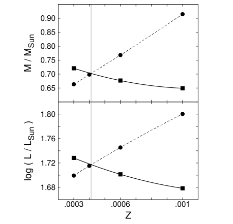
Figure 2: Stellar mass and luminosity as functions of the metallicity. Age and temperature are fixed at $\log(t[\mathrm{yr}])=7.424$ and $T_{\rm eff}=6851$ K. Continuous and dashed lines show the quadratic interpolants in Z for the evolutionary (squares) and pulsational (circles) models. For better visibility, the intersections are connected by a vertical grey line.

(a)

We construct isochrones from the solar-scaled horizontal branch models of Pietrinferni et al. (2004). Physical ingredients and details of the model building are described in their paper and references therein. Here we note only some relevant features. All models are canonical in the sense that they have been calculated without atomic diffusion and convective overshooting. They include up-to-date input physics, most importantly, they use recent and accurate results for plasma-neutrino processes and electron conduction opacities which lead to more accurate He core masses at evolutionary stages after the core helium flash. And last, but not least, their HB models have a fine mass spacing, particularly suitable for investigating stellar parameters in the instability strip.

(b)

From the pulsational solution (PS) we get ‘near straight lines’ for any fixed $T_{\rm eff}$ in the $Z~{}\rightarrow~{}(M,\log L)$ planes (hereafter ML planes).

(c)

For a given age we can search for the evolutionary solution (ES) by using the above fixed $T_{\rm eff}$. These solutions yield another set of ‘near straight lines’ in the ML planes.

(d)

The ES and PS lines may or may not intersect in the appropriate $Z$ range in the ML planes. If they do, then we have two $Z$ values at which intersection occurs. Obviously, the consistent $\mathrm{ES}=\mathrm{PS}$ solution should yield the same $Z$. Since this is generally not the case, the best solution is searched for by minimising the difference between the two metallicities:

$$\Delta Z = |\log Z_{M}-\log Z_{L}|\hskip 5.69054pt,$$ (3)

where $Z_{M}$ and $Z_{L}$ are the metallicities obtained in the M and L planes, respectively. To illustrate the solution obtained at a given age and temperature, we show the PS and ES curves and their intersections in Fig. 2. It is seen that these curves are indeed near linear. Therefore, we can employ quadratic interpolation to compute the positions of the intersections.

(e)

By changing the age, with the above method we can map the solution as a function of the evolutionary stage. As it follows from the above construction, at each stage we have different stellar parameters that yield the same periods and satisfy evolutionary constraints. The grey-scale plot of ${\Delta Z}$ on the $\log(t)$ — $T_{\rm eff}$ plane is shown in Fig. 3. It is remarkable how much the solution is limited in a narrow $T_{\rm eff}$ regime. It is also observable that we get solutions (i.e. ${\Delta Z}<10^{-4}$) at nearly all ages up to $\log(t)=7.77$ ($\approx 60$ Myr). We could, in principle, fix the age by using very accurately (and independently) determined $T_{\rm eff}$. However, the precision of the currently available methods for temperature estimation is insufficient for posing a strong constraint on the age.

Table 5: Physical parameters of BS Com derived in this paper

[Fe/H]	$T_{\rm eff}$   [K]	$M/M_{\odot}$	$\log(L/L_{\odot})$
$-1.67\pm 0.01$	$6840\pm 14$	$0.698\pm 0.004$	$1.712\pm 0.005$
$-1.58\pm 0.11$	$6842\pm 10$

Note: Errors for the ES/PS solution (first line) are the standard deviations of the various age-dependent solutions in the full age interval of $60$ Myr. Items derived from the $BVI_{\rm C}$ colours (second line) are taken from Table 3, errors are formal statistical ones.

The ridge line in Fig. 3 selects the best fitting models. The age dependencies of the corresponding $\log L$, $M$, and [Fe/H] are shown in Fig. 4. The small range of stellar parameters allowed by the solution is remarkable. The stronger topological change occurs at $\log t=7.6$ ($\approx 40$ Myr) just after the blueward loop where evolution starts toward the asymptotic giant branch. Considerably larger ages seem to be less probable because the associated high temperatures can be excluded by the ones derived from the colours. From the above result we can estimate the parameters of BS Com. Assuming equal probability of ages in the range plotted, we can compute the distributions of the various physical parameters. Although these distributions are not symmetric around their most probable values, for the present case this effect is of secondary importance and we compute the standard deviations around the averages as a first approximation of the errors introduced by the effect of age uncertainty. Table 5 displays the so-derived stellar parameters, which are compared with the independently estimated $T_{\rm eff}$ and [Fe/H] values from Table 3. It is reassuring that there is a comfortable overlap between the two sets of parameters, indicating a good level of consistency among the very different ingredients of the above parameter determination.

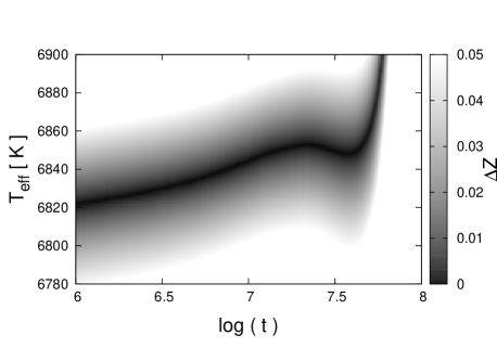
Figure 3: Grey-scale plot of the metallicity difference $\Delta Z$ [see Eq. (3)] on the age — $T_{\rm eff}$ plane.

Figure 4: Age dependence of the derived stellar parameters for BS Com.

The employment of the LNA pulsation models in the above solution presumes that the theoretical periods are applicable to the observed ones that are known to be inherently nonlinear due to the longevity of the observable double-mode state. Since our method strongly relies on this assumption, it is important to examine if the currently available nonlinear models predict some considerable change in the asymptotic nonlinear periods with respect to the LNA periods. We note that this problem is also present in any asteroseismological investigation if the multimode state is the result of some nonlinear phenomenon. However, nonlinear modelling is usually not easy to attempt since most of the multimode pulsators are of non-radial, therefore it would require full (i.e. 3D) hydrodynamics. We can pose the above question only in the case of RRd stars and double-mode Cepheids, since these variables are thought to be pure radial pulsators and we have successful nonlinear modelling available on these variables.

Data on the nonlinear/linear period difference for asymptotic hydrodynamical models are nearly non-existent. In an early assessment (Kovács, 2001b) we used the somewhat limited and preliminary result obtained by Kolláth & Buchler (2001). The nonlinear periods were longer than the linear ones in the order of $\sim\,0.001$ days. The amounts of the period shifts were such that they resulted in a decrease of less than $0.002$ in the period ratio. An ongoing, more extended study by Szabó et al. (to be published) basically confirms the above result. As it is detailed in Appendix C, we generated another set of LNA models by artificially decreasing the observed periods of BS Com by the amount predicted from the models of Szabó et al. After repeating the same computation as for the LNA periods, we ended up with stellar parameters that were remarkably close to the ones obtained with the LNA assumption. The solution curves (age vs. stellar parameters) exhibit small overall shifts that result in differences between the parameters obtained with the LNA and modified LNA solutions. The parameter shifts are approximately as follows: $+0.01$, $+0.006$, $+10$ K, $-0.08$, for $M/M_{\odot}$, $\log(L/L_{\odot})$, $T_{\rm eff}$ and [Fe/H], respectively, in the sense of modified LNA minus non-modified LNA. We conclude that considering the period shifts predicted by the currently available nonlinear simulations does not effect significantly the agreement with the independently estimated $T_{\rm eff}$ and [Fe/H].

6 Conclusions

We performed a pulsational/evolutionary analysis on one of the most extensively observed Galactic double-mode RR Lyrae (RRd) star BS Com. Our earlier analysis incorporating all of our measurements in the $BV(RI)_{\rm C}$ colours has shown that the light variation does not contain any other components except for those of the fundamental and first overtone modes together with their linear combinations (Dékány, 2007). Therefore, the presence of possible non-radial components is excluded above the $\sim$ mmag level. (This may not be the case for AQ Leo, where the analysis of the high precision data from the MOST satellite suggests the presence of two possibly non-radial components at the sub-mmag level – see Gruberbauer et al. 2007.) Based on the result of the frequency analysis, we decided to derive the physical parameters of BS Com using the assumption of radial double-mode pulsation.

Earlier studies on double-mode variables were mostly based on the period ratio (Petersen) diagram, which is an effective (but not complete) representation of the main (mass and heavy element) dependences of the periods (see e.g. Popielski et al., 2000). It is also possible to employ other available pieces of information, such as colour or overall cluster metallicity (e.g. Kovács, 2000a). In this paper we followed a purely theoretical approach, where we derived all basic stellar parameters by matching the evolutionary and pulsational properties. In the solutions age remains a free parameter.

It is important to confront the above theoretical solution with other independent pieces of information. For this goal, we utilised the observed $BVI_{\rm C}$ colours in deriving metal abundance and effective temperature with the help of updated solar-scaled stellar atmosphere models by Castelli (1999). We tested the reliability of the method through the comparison of the published spectroscopic abundances of 21 Galactic field fundamental mode RR Lyrae (RRab) stars. The standard deviation of the residuals between the spectroscopic and photometric metallicities is $0.15$ dex, which we consider as a good support for the reliability of the photometric method based on the $BVI_{\rm C}$ colours. By applying this method on BS Com, we get [Fe/H]$=-1.58\pm 0.11$, $T_{\rm eff}=6842\pm 10$ K, where the errors are purely statistical ones.

Taking into consideration the above independently estimated parameters, we can most probably exclude the late evolutionary stages after the core helium exhaustion. This is because the high temperature required by the solution is incompatible with the temperature computed from the observed colours. Therefore, in the acceptable set of solutions the age spans only an approximately 60 Myr range from the zero age horizontal branch till slightly after the start of the final redward evolution. Because we do not have independent information about the evolutionary status, all of these solutions are viable. However, the ranges covered by the parameters in the possible time interval are remarkably narrow. Furthermore, assuming uniform age distribution, most of the values are clumped in an even narrower regime at the earlier evolutionary stages. By considering this age ambiguity, we get $M/M_{\odot}=0.698\pm 0.004$, $\log(L/L_{\odot})=1.712\pm 0.005$, $T_{\rm eff}=6840\pm 14$ K, [Fe/H]=$-1.67\pm 0.01$ where the errors are $1\,\sigma$ ranges due to the above age interval.

It is interesting to compare the above values with the compilation of the average physical parameters of the RRd stars found in various stellar systems. In Table 2 of the paper by Kovács (2001a) we summarised the result for four systems, where the parameter determinations were performed without the use of evolutionary models. There are IC 4499 and LMC that have average metallicities similar to that of BS Com. Omitting LMC, due to its very wide population range, we see that the average RRd parameters in IC 4499 ($T_{\rm eff}=6760$ K, $\log L/L_{\odot}=1.708$, $M/M_{\odot}=0.755$) are remarkably similar to those of BS Com. The largest difference occurs in the mass, but this is due to the slightly longer period of BS Com than the average value of the RRd stars in IC 4499. Since the other stellar parameters are nearly the same, this period difference results in a larger average mass for the cluster stars.

Another indirect check of the consistency of our theoretical parameters of BS Com is the computation of the zero point of the period-luminosity-colour (PLC) relation of Kovács & Walker (2001). Although this relation was derived from fundamental mode RR Lyrae stars, because of its apparent generality, we use it with the period of the fundamental mode of BS Com. By using $M_{\rm bol,\odot}=4.75$, a bolometric correction interpolated to the appropriate stellar parameters of ${\rm BC}=-0.15$ (see Castelli, 1999) and a reddening value given by Schlegel et al. (1998, see Table 3), we get $-1.02$ for the PLC zero point. In comparing this value with the one published by Kovács (2003), we see that the above value is larger by $0.06$, yielding lower distance modulus for the LMC by the same amount (we recall that the LMC distance modulus with the zero point of Kovács (2003) comes out to be $18.55$). We think that the above result confirms the consistency of the derived physical parameters, especially if we add the ambiguity due to the yet to be shown fit of the RRd variables to the PLC relation derived from RRab stars.

We have also tested the effect of a possible period shift due to convection and nonlinearity. Based on the extensive set of models by Szabó et al. (in preparation), our conclusion is that the effect in the derived parameters is relatively small ($\sim\,1.5\,\%$). Once this correction is proved to be important by future studies, taking it into consideration is fairly easy, since the overall period shift seems to be almost independent of the particular model parameters. Therefore, there is no need to run specific nonlinear models in each case but it is quite enough to fit the relatively inexpensive linear models to the modified periods based on the above general corrections.

The remarkably small ambiguity of the derived stellar parameters from the purely theoretical method employed in this paper brings up several intriguing questions. One of these is the compatibility of the theoretical abundance and temperature and the ones obtained by spectroscopic and various semi-empirical methods (e.g. by the widely used infrared flux method). Accuracies such as $1\%$ (or better) are quoted for the temperature in the current papers on this topic (e.g. Masana, Jordi & Ribas, 2006). Unfortunately, for the chemical composition we still lack this level of accuracy. Most of the abundances available for RR Lyrae stars are based on some calibration of low-dispersion spectra by a low number of high-dispersion ones. Double-mode stars in globular clusters are obvious targets for the above-type of studies, due to the expected chemical homogeneity and same distance. Last, but not least, we note the need of putting more stringent constraints on the nonlinear hydrodynamical models. Our current understanding is that double-mode behaviour is caused by the non-resonant interaction of two normal modes with a delicate level of physical dissipation (understood as the result of convection). Although the global observational and theoretical properties are in reasonable agreement, the accuracy of the presently available stellar parameters is insufficient to lend further support to these models. Considering the general astrophysical importance of convection and, in particular, the role of that in double-mode pulsation, it is clear that pinning down the physical parameters is of great significance.

Appendix A Fourier decomposition of BS Comae

Table 6 shows the frequencies, amplitudes and phases of the 15-term Fourier sum fitted to the light curves of BS Com. Phases refer to sine-term decomposition with an epoch $t_{0}=2453431.0$. The Fourier-sums fit the $B,V,R_{C},I_{\mathrm{C}}$ data with $0.0116$, $0.0097$, $0.0091$, $0.0098$ mag rms scatters, respectively. These values are in the appropriate proximity of the formal errors of the individual photometric data points as derived from the IRAF package. To determine the errors of the fitted amplitudes and phases, we performed Monte Carlo simulations of the light curves. Synthetic data were generated by adding independent Gaussian random noise to the Fourier solution, with $\sigma$ made equal to the rms scatter of the residual data. Errors in Table 6 are the standard deviations of the Fourier parameters obtained from 100 independent realisations of the light curve in each colour.

Table 6: Fourier decompositions of the $B,V,R_{\rm C},I_{\rm C}$ light curves of BS Com.

Identification		Frequency	$A_{B}$	$A_{V}$	$A_{R_{\mathrm{C}}}$	$A_{I_{\mathrm{C}}}$
$f_{0}$	–	$2.04955$	$164.26\pm 0.77$	$127.05\pm 0.47$	$101.18\pm 0.45$	$79.63\pm 0.51$
$2f_{0}$	–	$4.09910$	$26.51\pm 0.70$	$20.87\pm 0.47$	$17.26\pm 0.46$	$14.88\pm 0.48$
$3f_{0}$	–	$6.14865$	$4.43\pm 0.78$	$1.82\pm 0.47$	$1.44\pm 0.45$	$2.48\pm 0.47$
–	$f_{1}$	$2.75432$	$259.43\pm 0.76$	$201.66\pm 0.46$	$161.36\pm 0.42$	$123.06\pm 0.51$
–	$2f_{1}$	$5.50864$	$35.55\pm 0.83$	$29.08\pm 0.49$	$22.76\pm 0.50$	$17.42\pm 0.47$
–	$3f_{1}$	$8.26296$	$15.57\pm 0.68$	$12.48\pm 0.46$	$9.87\pm 0.49$	$6.86\pm 0.44$
–	$4f_{1}$	$11.01728$	$3.75\pm 0.65$	$3.21\pm 0.42$	$2.94\pm 0.45$	$2.48\pm 0.47$
$f_{0}$	$f_{1}$	$4.80387$	$62.50\pm 0.65$	$50.23\pm 0.48$	$40.87\pm 0.54$	$32.82\pm 0.54$
$f_{0}$	$-f_{1}$	$0.70477$	$36.19\pm 0.68$	$29.65\pm 0.43$	$24.98\pm 0.49$	$18.10\pm 0.53$
$2f_{0}$	$f_{1}$	$6.85342$	$11.59\pm 0.78$	$9.75\pm 0.51$	$8.54\pm 0.42$	$6.86\pm 0.52$
$f_{0}$	$2f_{1}$	$7.55819$	$21.67\pm 0.74$	$20.31\pm 0.47$	$15.30\pm 0.49$	$11.38\pm 0.57$
$2f_{0}$	$2f_{1}$	$9.60774$	$10.85\pm 0.77$	$6.08\pm 0.46$	$4.99\pm 0.41$	$3.14\pm 0.45$
$f_{0}$	$3f_{1}$	$10.31251$	$8.04\pm 0.79$	$6.46\pm 0.46$	$4.28\pm 0.42$	$3.61\pm 0.50$
$f_{0}$	$-3f_{1}$	$6.21341$	$5.09\pm 0.83$	$2.63\pm 0.50$	$3.52\pm 0.47$	$2.24\pm 0.50$
$f_{0}$	$4f_{1}$	$13.06683$	$3.35\pm 0.56$	$2.56\pm 0.45$	$1.78\pm 0.43$	$1.46\pm 0.43$
			$\Phi_{B}$	$\Phi_{V}$	$\Phi_{R_{\rm C}}$	$\Phi_{I_{\rm C}}$
–	$f_{1}$	$2.754320$	$3.121\pm 0.004$	$3.080\pm 0.004$	$3.034\pm 0.005$	$2.960\pm 0.006$
–	$2f_{1}$	$5.508640$	$2.255\pm 0.030$	$2.199\pm 0.019$	$2.304\pm 0.026$	$2.210\pm 0.032$
–	$3f_{1}$	$8.262960$	$1.023\pm 0.176$	$1.562\pm 0.273$	$2.202\pm 0.355$	$1.433\pm 0.260$
–	$4f_{1}$	$11.017280$	$2.216\pm 0.003$	$2.200\pm 0.003$	$2.172\pm 0.003$	$2.104\pm 0.004$
$f_{0}$	–	$2.049550$	$1.560\pm 0.020$	$1.534\pm 0.016$	$1.502\pm 0.019$	$1.569\pm 0.030$
$2f_{0}$	–	$4.099100$	$0.438\pm 0.046$	$0.433\pm 0.035$	$0.426\pm 0.048$	$0.457\pm 0.074$
$3f_{0}$	–	$6.148650$	$5.553\pm 0.180$	$5.992\pm 0.133$	$5.746\pm 0.137$	$5.727\pm 0.169$
$f_{0}$	$f_{1}$	$4.803870$	$1.564\pm 0.014$	$1.576\pm 0.008$	$1.602\pm 0.013$	$1.542\pm 0.014$
$f_{0}$	$-f_{1}$	$0.704770$	$4.576\pm 0.022$	$4.616\pm 0.015$	$4.657\pm 0.018$	$4.682\pm 0.024$
$2f_{0}$	$f_{1}$	$6.853420$	$0.875\pm 0.054$	$0.829\pm 0.046$	$0.931\pm 0.059$	$0.793\pm 0.066$
$f_{0}$	$2f_{1}$	$7.558190$	$0.234\pm 0.035$	$0.251\pm 0.023$	$0.250\pm 0.027$	$0.316\pm 0.045$
$2f_{0}$	$2f_{1}$	$9.607740$	$0.319\pm 0.071$	$0.159\pm 0.077$	$0.113\pm 0.071$	$0.178\pm 0.135$
$f_{0}$	$3f_{1}$	$10.312510$	$0.698\pm 0.097$	$0.359\pm 0.082$	$0.102\pm 0.109$	$6.266\pm 0.114$
$f_{0}$	$-3f_{1}$	$6.213410$	$4.988\pm 0.162$	$5.180\pm 0.199$	$5.342\pm 0.145$	$5.418\pm 0.236$
$f_{0}$	$4f_{1}$	$13.066830$	$5.980\pm 0.164$	$5.303\pm 0.170$	$5.341\pm 0.232$	$4.824\pm 0.358$

Notes: The light curves are represented in the from of $A_{0}+A_{1}\cdot\sin(2\pi f(t-t_{0})+\Phi_{1})+\dots$
with $t_{0}=2453431.0$. Frequency is given in d^-1, amplitudes and phases are in mmag and radians, respectively. We show $1\sigma$ formal statistical errors.

Appendix B The sample for testing the $\mathbf{BVI_{C}}~{}-~{}\mathbf{[Fe/H],T_{eff}}$ relation

Here we present the parameters of the 24 RRab used in Sect. 3 to test the method of metallicity and temperature estimation from the $BVI_{\rm C}$ colours and fundamental periods. Table 7 shows fundamental periods, colour indices, interstellar reddenings and spectroscopic [Fe/H]_sp values taken from the literature. We relied mainly on the compilations by Kovács & Jurcsik (1997) for colour indices and on Jurcsik & Kovács (1996) for [Fe/H], except for three stars. For the abundances of UU Cet and V440 Sgr we refer to Clementini et al. (1995a) and for RV Phe to Jones (1973). Reddenings were taken from Blanco (1992), except for BB Pup for which we used the E($B-V$) value given by Schlegel et al. (1998). The derived [Fe/H]_ph photometric abundances for each star are listed in the last column of Table 7. For X Ari, SS Leo, and VY Ser, we get discrepant [Fe/H]_ph values. These might be due to systematic errors in their colour indices, which have a particularly large effect on the estimated [Fe/H]_ph at lower metallicities (see Kovács 2008). We also note that SS Leo and VY Ser have also been met as outliers in various earlier studies (e.g. Kovács & Kanbur, 1998; Kovács & Walker, 2001; Kovács, 2003).

Table 7: Properties of the test RRab stars

Star	$P_{\mathrm{F}U}$	$B-V$	$V-I_{\mathrm{C}}$	$\mathrm{E}(B-V)$	[Fe/H]sp	[Fe/H]ph
SW And	$0.4422659$	$0.434$	$0.544$	$0.09$	$-0.06$	$-0.22$
WY Ant	$0.5743365$	$0.384$	$0.549$	$0.05$	$-1.39$	$-1.13$
X Ari	$0.6511597$	$0.490$	$0.724$	$0.16$	$-2.10$	$-2.50$
RR Cet	$0.5530288$	$0.371$	$0.537$	$0.05$	$-1.29$	$-1.28$
UU Cet	$0.6053409$	$0.390$	$0.567$	$0.01$	$-1.38$	$-1.33$
W Crt	$0.4120139$	$0.370$	$0.466$	$0.09$	$-0.45$	$-0.22$
DX Del	$0.4726182$	$0.454$	$0.571$	$0.09$	$-0.32$	$-0.26$
SU Dra	$0.6604200$	$0.348$	$0.519$	$0.02$	$-1.56$	$-1.50$
SW Dra	$0.5696710$	$0.369$	$0.520$	$0.01$	$-0.95$	$-0.93$
RX Eri	$0.5872475$	$0.415$	$0.585$	$0.10$	$-1.07$	$-1.13$
RR Gem	$0.3973082$	$0.406$	$0.511$	$0.11$	$-0.14$	$-0.23$
RR Leo	$0.4523926$	$0.334$	$0.486$	$0.03$	$-1.30$	$-1.23$
SS Leo	$0.6263438$	$0.350$	$0.488$	$0.02$	$-1.56$	$-0.82$
TT Lyn	$0.5974332$	$0.381$	$0.550$	$0.05$	$-1.50$	$-1.26$
V445 Oph	$0.3970232$	$0.620$	$0.772$	$0.29$	$+0.01$	$-0.18$
AV Peg	$0.3903760$	$0.424$	$0.528$	$0.10$	$+0.08$	$-0.17$
AR Per	$0.4255489$	$0.676$	$0.853$	$0.35$	$-0.14$	$-0.31$
RV Phe	$0.5964182$	$0.370$	$0.535$	$0.03$	$-1.50$	$-1.19$
BB Pup	$0.4805468$	$0.459$	$0.582$	$0.11$	$-0.35$	$-0.47$
V440 Sgr	$0.4774788$	$0.404$	$0.568$	$0.09$	$-1.14$	$-1.09$
VY Ser	$0.7140962$	$0.377$	$0.579$	$0.02$	$-1.71$	$-2.33$
W Tuc	$0.6422370$	$0.329$	$0.490$	$0.01$	$-1.37$	$-1.39$
TU UMa	$0.5576570$	$0.364$	$0.522$	$0.05$	$-1.15$	$-1.15$
UU Vir	$0.4756062$	$0.349$	$0.475$	$0.02$	$-0.60$	$-0.66$

Note: Periods are in [days], colour indices and reddenings are in [mag]. See Appendix B for references on the sources of data.

Appendix C Effect of nonlinearity

Table 8: Pulsation models matching the modified periods of BS Com

$T_{\rm eff}$	$M$	$\log L$	$R$	$\log g$	$\log\rho$
		$X=0.7547$		$Z=0.0003$
6700	0.672	1.662	5.026	2.862	$-2.128$
6750	0.679	1.679	5.050	2.863	$-2.129$
6800	0.689	1.697	5.080	2.864	$-2.131$
6850	0.697	1.714	5.105	2.865	$-2.132$
6900	0.707	1.732	5.137	2.866	$-2.134$
		$X=0.7546$		$Z=0.0004$
6700	0.705	1.677	5.114	2.868	$-2.130$
6750	0.715	1.695	5.144	2.869	$-2.131$
6800	0.724	1.713	5.172	2.870	$-2.133$
6850	0.733	1.730	5.200	2.871	$-2.134$
6900	0.745	1.748	5.232	2.872	$-2.135$
		$X=0.7534$		$Z=0.0006$
6700	0.772	1.706	5.287	2.879	$-2.133$
6750	0.786	1.725	5.325	2.881	$-2.135$
6800	0.798	1.743	5.356	2.882	$-2.136$
6850	0.810	1.761	5.389	2.883	$-2.138$
6900	0.820	1.778	5.416	2.884	$-2.139$
		$X=0.7530$		$Z=0.0010$
6700	0.919	1.761	5.633	2.900	$-2.140$
6750	0.930	1.778	5.660	2.901	$-2.141$
6800	0.944	1.796	5.694	2.902	$-2.142$
6850	0.959	1.814	5.728	2.903	$-2.144$
6900	0.971	1.831	5.757	2.904	$-2.145$

Notes: $T_{\rm eff}$ is given in [K], $M$, $\log L$ and $R$ are measured in solar units, $g$ and $\rho$ are in [CGS]. Observed periods match within $10^{-5}$ d. The modified periods are $P_{0}=0.486448$ and $P_{1}=0.362340$ days.

In Szabó et al. (in preparation) we examine the period shifts between the asymptotic nonlinear period of the convective models and those of the purely radiative linear non-adiabatic models (i.e. the ones we use in this paper). The results are based on many different models, including various combinations of physical and model construction parameters (notably depth of the inner boundary and number of mass shells constituting the stellar model). All models show that both modes have longer periods in the asymptotic double-mode regime than those in the LNA approximation. The amount of period increase is smaller than $0.001$ days. The shifts lead to period ratio values that are lower by up to $0.0015$ than the LNA ones. For the overall relative period shifts we get:

$$P_{\rm LNA}(FU)/P_{\rm NL}(FU) = 0.997$$ (4)

$$P_{\rm LNA}(FO)/P_{\rm NL}(FO) = 0.998~{}.$$ (5)

Assuming that the observed periods of BS Com correspond to the nonlinear asymptotic values, the predicted modified LNA values are as follows:

$$P_{0}(\rm{LNA},mod.) = 0.486448$$ (6)

$$P_{1}(\rm{LNA},mod.) = 0.362340$$ (7)

$$P_{1}/P_{0}(\rm{LNA},mod.) = 0.744869~{}.$$ (8)

With these periods we performed the same type of LNA survey as described in Sect. 5 for the observed periods. The result is shown in Table C1. By comparing the items at the same chemical composition and temperature with those matching the observed periods, we see that $M$ and $\log L$ are shifted to larger values by $\sim\,0.04$ and $\sim\,0.015$, respectively. However, in the final solution the difference between the parameters obtained by the predicted and directly computed LNA periods will be considerably smaller, due to the compensating effect of changes in $T_{\rm eff}$ and [Fe/H] (see Sect. 5 for additional details).

References

- Alexander & Ferguson (1994) Alexander D. R., Ferguson J. W., 1994, ApJ, 437, 879
- Bakos (1999) Bakos G. Á., 1999, Konkoly Obs. Occ. Techn. Notes, 11 http://www.konkoly.hu/Mitteilungen/Mitteilungen.html
- Benedict et al. (2007) Benedict G. F. et al. 2007, AJ, 133, 1810
- Blanco (1992) Blanco V. M., 1992, AJ, 104, 734
- Bono et al. (1995) Bono G., Caputo F., Stellingwerf R. F., 1995, ApJS, 99, 263
- Buchler (1990) Buchler J. R., 1990, NATO ASI series, 302, 1
- Buchler & Szabó (2007) Buchler J. R., Szabó R., 2007, ApJ, 660, 723
- Castelli (1999) Castelli F., 1999, A&A, 346, 564
- Castelli et al. (1997) Castelli F., Gratton R. G., Kurucz R. L., 1997, A&A, 318, 841
- Castor (1971) Castor J. I., 1971, ApJ, 166, 109
- Clementini et al. (1995a) Clementini G., Carretta E., Gratton R., Merighi R., Mould J. R., McCarthy J. K., 1995a, AJ, 110, 2319
- Clementini et al. (1995b) Clementini G., Tosi M., Bragaglia A., Merighi R., Maceroni C., 1995b, MNRAS, 275, 929
- Cox (1991) Cox A. N., 1991, ApJ, 381, L71
- Dékány (2007) Dékány I., 2007, AN, 328, 833
- Feuchtinger (1998) Feuchtinger M. U., 1998, A&A, 337, L29
- Fouqué et al. (2007) Fouque P. et al., 2007, A&A, 476, 73
- Garcia-Melendo & Clement (1997) Garcia-Melendo E., Clement C. M., 1997, AJ, 114, 1190
- Grevesse & Anders (1991) Grevesse N., Anders E., 1991, in Solar interior and atmosphere. University of Arizona Press, 1991, p. 1227
- Grevesse & Sauval (1998) Grevesse N., Sauval A. J., 1998, Space Sci. Rev., 85, 161
- Gruberbauer et al. (2007) Gruberbauer M. et al., 2007, MNRAS, 379, 1498
- Holtzman & Nations (1984) Holtzman J. A., Nations H. L., 1984, AJ, 89, 391
- Iglesias & Rogers (1996) Iglesias C. A., Rogers F. J., 1996, ApJ, 464, 943
- Jones (1973) Jones D. H. P., 1973, ApJS, 25, 487
- Jurcsik (1995) Jurcsik J., 1995, AcA, 45, 653
- Jurcsik & Kovács (1996) Jurcsik J., Kovács G., 1996, A&A, 312, 111
- Kolláth et al. (1998) Kolláth Z., Beaulieu J. P., Buchler J. R., Yecko P., 1998, ApJ, 502, L55
- Kolláth & Buchler (2001) Kolláth Z., Buchler J. R., 2001, ASSL, 257, 29
- Kovács (2000a) Kovács G., 2000a, A&A, 360, L1
- Kovács (2000b) Kovács G., 2000b, A&A, 363, L1
- Kovács (2001a) Kovács G., 2001a, A&A, 375, 469
- Kovács (2001b) Kovács G., 2001b, ASSL, 257, 61
- Kovács (2003) Kovács G., 2003, MNRAS, 342, L58
- Kovács (2006) Kovács G., 2006, MmSAI, 77, 160
- Kovács (2008) Kovács G., 2008, to appear in Goupil M. J. et al., eds, Nonlinear Stellar Hydrodynamics and Pulsations of Cepheids, EDP Sci.
- Kovács & Buchler (1993) Kovács G., Buchler J. R., 1993, ApJ, 404, 765
- Kovács & Jurcsik (1997) Kovács G., Jurcsik J., 1997, A&A, 322, 218
- Kovács & Kanbur (1998) Kovács G., Kanbur S. M., 1998, MNRAS, 295, 834
- Kovács & Walker (1999) Kovács G., Walker A. R., 1999, ApJ, 512, 271
- Kovács & Walker (2001) Kovács G., Walker A. R., 2001, A&A, 371, 579
- Kovács et al. (1992) Kovács G., Buchler J. R., Marom A., Iglesias C. A., Rogers F. J., 1992, A&A, 259, L46
- Lub (1979) Lub J., 1979, AJ, 84, 383
- Masana et al. (2006) Masana E., Jordi C., Ribas I., 2006, A&A, 450, 735
- McNamara et al. (2007) McNamara D. H., Clementini G., Marconi M., 2007, AJ, 133, 2752
- Mizerski (2003) Mizerski T., 2003, AcA, 53, 307
- Moskalik & Poretti (2003) Moskalik P., Poretti E., 2003, A&A, 398, 213
- Nagy & Kovács (2006) Nagy A., Kovács G., 2006, A&A, 454, 257
- Pietrinferni et al. (2004) Pietrinferni A., Cassisi S., Salaris M., Castelli F., 2004, ApJ, 612, 168
- Pigulski et al. (2003) Pigulski A., Kolaczkowski Z., Kopacki G., 2003, AcA, 53, 27
- Popielski et al. (2000) Popielski B. L., Dziembowski W. A., Cassisi S., 2000, AcA, 50, 491
- Rogers & Iglesias (1992) Rogers F. J., Iglesias C. A., 1992, ApJS, 79, 507
- Schlegel et al. (1998) Schlegel D. J., Finkbeiner D. P., Davis M., 1998, ApJ, 500, 525
- Seaton et al. (1994) Seaton M. J., Yan Y., Mihalas D., Pradhan A. K., 1994, MNRAS, 266, 805
- Simon (1982) Simon N. R., 1982, ApJ, 260, L87
- Smith (1990) Smith H. A., 1990, PASP, 102, 124
- Sódor (2007) Sódor Á., 2007, AN, 328, 829
- Sozzetti et al. (2007) Sozzetti A., Torres G., Charbonneau D., Latham D. W., Holman M. J., Winn J. N., Laird J. B., O’Donovan F. T., 2007, ApJ, 664, 1190
- Stellingwerf (1975) Stellingwerf R. F., 1975, ApJ, 195, 441
- Storm et al. (2004) Storm J., Carney B. W., Gieren W. P., Fouqué P., Latham D. W., Fry A. M., 2004, A&A, 415, 531
- Sturch (1966) Sturch C., 1966, ApJ, 143, 774
- Szabó et al. (2004) Szabó R., Kolláth Z., Buchler J. R., 2004, A&A, 425, 627
- Twarog et al. (2003) Twarog B. A., Anthony-Twarog B. J., De Lee N., 2003, AJ, 125, 1383
- van Leeuwen et al. (2007) van Leeuwen F., Feast M. W., Whitelock P. A., Laney C. D., 2007, MNRAS, 379, 723
- Wils (2006) Wils P., 2006, IBVS, 5685, 1