ABOUT THE TRUE TYPE OF SMOOTHERS

Abstract

We employ the variational formulation and the Euler-Lagrange equations to study the steady-state error in linear non-causal estimators (smoothers). We give a complete description of the steady-state error for inputs that are polynomial in time. We show that the steady-state error regime in a smoother is similar to that in a filter of double the type. This means that the steady-state error in the optimal smoother is significantly smaller than that in the Kalman filter. The results reveal a significant advantage of smoothing over filtering with respect to robustness to model uncertainty.

Keywords: Linear smoothing, steady state error, type

1 Introduction

The appearance of steady-state errors is endemic in linear and nonlinear tracking systems and was extensively studied in control theory [5]. An important result from linear deterministic control theory is that the tracking properties of a closed-loop control system are determined by its type. The type of the system is defined as the number of pure integrators in the transfer function of the system within the closed loop. A type-$n$ system can track a polynomial input of the form $a\displaystyle\frac{t^{(p-1)}}{(p-1)!}$ without any steady-state error for $p\leq n$, with constant steady-state error for $p=n+1$, and cannot track the input signal for $p>n+1$. This result is easily obtained using the final value theorem [5] from Laplace transform theory.

Another result from estimation theory is that a Kalman filter [8], designed for the $n$-th order model

$$\begin{array}[]{lll}\displaystyle\frac{d^{n}x}{dt^{n}}&=&x^{(n)}=\sigma\,\dot{w}\\ &&\\ y&=&x+\rho\,\dot{v},\end{array}$$ (4)

where $w(t)$ and $v(t)$ are independent Brownian motions, results in a type-$n$ closed-loop tracking system (as demonstrated below). Combining the above results and using the linearity of the Kalman filter, implies that a Kalman filter designed for the $n$-th order model (4) tracks the signal

$$\tilde{x}^{(n)}=\sigma\,\dot{w}+a\frac{t^{m}}{m!}$$ (5)

with constant steady state error for $m=0$, and cannot track the input signal for $m>0$.

Although a steady-state error is a fundamental concept in tracking and control theory, the appearance of steady-state errors in non-causal estimators (smoothers) has never been addressed, despite the extensive study of linear and nonlinear smoothers in the literature [12, 13, 14, 10, 17, 3, 2, 15, 16, 7, 11, 1]. The purpose of this paper is to fill the gap in the theory and to give a complete description of the steady-state error regime in linear smoothers. Specifically, we compute the steady-state error in the linear minimum mean square error (MMSE) smoother, designed for the model (4). We show that the steady-state error in the smoother is similar to that in the corresponding filter of double the type. Questions of convergence and stability of fixed interval smoothers were considered recently in [6].

2 Mathematical preliminaries

We begin with the general linear signal and measurement model

$$\begin{array}[]{lll}\dot{\mbox{\boldmath$x$}}&=&\mbox{\boldmath$A$}\mbox{\boldmath$x$}+\mbox{\boldmath$G$}\dot{\mbox{\boldmath$w$}}\\ &&\\ \mbox{\boldmath$y$}&=&\mbox{\boldmath$H$}\mbox{\boldmath$x$}+\mbox{\boldmath$B$}\dot{\mbox{\boldmath$v$}},\end{array}$$ (9)

where $\mbox{\boldmath$w$}(t),\ \mbox{\boldmath$v$}(t)$ are orthogonal vectors of independent Brownian motions. The minimum mean square estimation error (MMSEE) or maximum a-posteriori (MAP) estimator $\hat{\mbox{\boldmath$x$}}(\cdot)$ of $\mbox{\boldmath$x$}(\cdot)$, conditioned on the measurement $\mbox{\boldmath$y$}(\cdot)$, is the minimizer over all square integrable functions $u$ of the integral quadratic cost functional [3, 2]

$$\int_{0}^{T}\left[(\mbox{\boldmath$y$}-\mbox{\boldmath$Hz$})^{T}(\mbox{\boldmath$BB$}^{T})^{-1}(\mbox{\boldmath$y$}-\mbox{\boldmath$Hz$})+\mbox{\boldmath$u$}^{T}\mbox{\boldmath$u$}\right]\,dt,$$ (10)

subject to the equality constraint

$$\dot{\mbox{\boldmath$z$}}=\mbox{\boldmath$Az$}+\mbox{\boldmath$Gu$},$$ (11)

where $[0,T]$ is the observation interval. Note that the first term in (10) represents the energy of the measurements noise associated with the test function $\mbox{\boldmath$z$}(\cdot)$, while the second term represents that of the driving noise associated with $\mbox{\boldmath$z$}(\cdot)$. Note further that the integral in (10) contains the white noises $\dot{\mbox{\boldmath$w$}}(t),\ \dot{\mbox{\boldmath$v$}}(t)$, which are not square integrable. To remedy this problem, we proceed in the standard way [4] by beginning with a model in which the white noises $\dot{\mbox{\boldmath$w$}}(t),\ \dot{\mbox{\boldmath$v$}}(t)$ are replaced with square integrable wide band noises, and at the appropriate stage of the analysis, we take the white noise limit.

The Euler-Lagrange (EL) equations [9] for the minimizer $\hat{\mbox{\boldmath$x$}}=\hat{\mbox{\boldmath$x$}}(t\,|\,T)$ of the problem (10), (11) are

$$\begin{array}[]{lll}\displaystyle\frac{\partial\hat{\mbox{\boldmath$x$}}(t\,|\,T)}{\partial t}&=&\mbox{\boldmath$A$}\hat{\mbox{\boldmath$x$}}(t\,|\,T)-\displaystyle\frac{1}{2}\mbox{\boldmath$GG$}^{T}\mbox{\boldmath$\lambda$}\\ &&\\ \dot{\mbox{\boldmath$\lambda$}}&=&-2\mbox{\boldmath$H$}^{T}(\mbox{\boldmath$BB$}^{T})^{-1}\mbox{\boldmath$H$}\hat{\mbox{\boldmath$x$}}(t\,|\,T)-\mbox{\boldmath$A$}^{T}\mbox{\boldmath$\lambda$}+2\mbox{\boldmath$H$}^{T}(\mbox{\boldmath$BB$}^{T})^{-1}\mbox{\boldmath$y$}(t),\end{array}$$ (15)

with the boundary conditions

$$\hat{\mbox{\boldmath$x$}}(0\,|\,T)=\mbox{\boldmath$x$}_{0},\ \ \ \ \ \mbox{\boldmath$\lambda$}(T)=0.$$ (16)

Thus, the estimation problem is reduced to a linear two-point boundary-value problem, which is solved in closed form by the sweep method. Specifically, first the signal is filtered causally by the Kalman filter $\hat{\mbox{\boldmath$x$}}(t)$, satisfying

$$\dot{\hat{\mbox{\boldmath$x$}}}(t) = \mbox{\boldmath$A$}\hat{\mbox{\boldmath$x$}}(t)+\mbox{\boldmath$P$}\mbox{\boldmath$H$}^{T}(\mbox{\boldmath$BB$}^{T})^{-1}[\mbox{\boldmath$y$}(t)-\mbox{\boldmath$H$}\hat{\mbox{\boldmath$x$}}(t)],$$ (17)

and $\mbox{\boldmath$P$}(t)$ is the covariance matrix, satisfying the Riccati equation

$$\dot{\mbox{\boldmath$P$}}=\mbox{\boldmath$AP$}+\mbox{\boldmath$PA$}^{T}+\mbox{\boldmath$GG$}^{T}-\mbox{\boldmath$PH$}^{T}(\mbox{\boldmath$BB$}^{T})^{-1}\mbox{\boldmath$HP$}.$$ (18)

Then the smoother $\hat{\mbox{\boldmath$x$}}(t\,|\,T)$ is the backward sweep of the Kalman filter,

$$\displaystyle\frac{\partial\hat{\mbox{\boldmath$x$}}(t\,|\,T)}{\partial t}=\mbox{\boldmath$A$}\hat{\mbox{\boldmath$x$}}(t\,|\,T)+\mbox{\boldmath$GG$}^{T}\mbox{\boldmath$P$}^{-1}[\hat{\mbox{\boldmath$x$}}(t\,|\,T)-\hat{\mbox{\boldmath$x$}}(t)],$$ (19)

with the boundary condition

$$\hat{\mbox{\boldmath$x$}}(T\,|\,T)=\hat{\mbox{\boldmath$x$}}(T).$$ (20)

We continue with the steady-state error regime in the Kalman filter designed for the $n$-th order model (4). Rewriting (4) in vector matrix notation leads to

$$\begin{array}[]{lll}\dot{\mbox{\boldmath$x$}}&=&\mbox{\boldmath$A$}\mbox{\boldmath$x$}+\sigma\mbox{\boldmath$b$}\dot{w}\\ &&\\ y&=&\mbox{\boldmath$h$}^{T}\mbox{\boldmath$x$}+\rho\,\dot{v},\end{array}$$ (24)

where $\mbox{\boldmath$x$}=[x,x_{2},\ldots,x_{n}]^{T}$, and

$$\mbox{\boldmath$A$}=\left[\begin{array}[]{cccccc}0&1&0&0&\ldots&0\\ 0&0&1&0&\ldots&0\\ 0&0&0&1&\ldots&0\\ &&\vdots&&&\\ 0&0&0&0&\ldots&0\end{array}\right];\quad\mbox{\boldmath$b$}=\left[\begin{array}[]{c}0\\ 0\\ \vdots\\ 0\\ 1\end{array}\right];\quad\mbox{\boldmath$h$}=\left[\begin{array}[]{c}1\\ 0\\ \vdots\\ 0\\ 0\end{array}\right].$$

The Kalman filter estimator $\hat{\mbox{\boldmath$x$}}(t)=[\hat{x}(t),\hat{x}_{2}(t),\ldots,\hat{x}_{n}(t)]^{T}$ for the model (24) satisfies (see equation (17)

$$\dot{\hat{\mbox{\boldmath$x$}}}(t)=\mbox{\boldmath$A$}\hat{\mbox{\boldmath$x$}}(t)+\mbox{\boldmath$k$}[y(t)-\hat{x}(t)],$$ (26)

where $\mbox{\boldmath$k$}(t)=[k_{1}(t),\ldots,k_{n}(t)]^{T}=\displaystyle\frac{1}{\rho^{2}}\mbox{\boldmath$P$}(t)\mbox{\boldmath$h$}$. The equation of the Kalman filter (26) may be rewritten in the form

$$\begin{array}[]{lll}\dot{\hat{x}}(t)&=&\hat{x}_{2}(t)+k_{1}[y(t)-\hat{x}(t)]\\ &\vdots&\\ \dot{\hat{x}}_{n-1}(t)&=&\hat{x}_{n}(t)+k_{n-1}[y-\hat{x}(t)]\\ &&\\ \dot{\hat{x}}_{n}(t)&=&k_{n}[y-\hat{x}(t)],\end{array}$$ (32)

which form a type-$n$ closed-loop tacking system with input $y(t)$, output $\hat{x}(t)$ and open-loop transfer function

$$G(S)=\frac{k_{1}S^{n-1}+k_{2}S^{n-2}+\ldots+k_{n}}{S^{n}}.$$ (33)

Thus, the Kalman filter designed for the $n$-th order model (4) tracks the signal

$$\tilde{x}^{(n)}=\sigma\,\dot{w}+a\frac{t^{m}}{m!}$$ (34)

with constant steady state error for $m=0$, and cannot track the input signal for $m>0$. The the terminology offset case $m=0$ of filtering theory is kept also for smoothing.

3 Steady-state errors in smoothers

Having described the steady-state error phenomenon in the Kalman filters, we continue with the evaluation of the steady-state errors in smoothers. We assume that a linear smoother is designed for the $n$-th order signal model (4), for which the Kalman filter was designed in the previous section. In order to examine the tracking properties of the smoother, we assume that the incoming signal is augmented with a $(n+m)-$th order polynomial in $t$

$$\begin{array}[]{lll}\tilde{x}^{(n)}&=&\displaystyle\frac{at^{m}}{m!}+\sigma\,\dot{w}\\ &&\\ y&=&\tilde{x}+\rho\,\dot{v}.\end{array}$$ (38)

For the sake of simplicity, we assume hereafter that $\sigma=\rho=\sqrt{\varepsilon}$ and $\tilde{x}(0)=\hat{x}(0)=0$. The smoother is a linear system, so the response of the smoother to the measurement signal $y(t)$ can be separated into a deterministic term, depending on the drift $\displaystyle\frac{at^{m}}{m!}$, and a stochastic term depending on $w(t),\,v(t)$. Because the steady-state error regime is determined by the deterministic term, we consider the noiseless version of (38)

$$\begin{array}[]{lll}\tilde{x}^{(n)}&=&\displaystyle\frac{at^{m}}{m!}\\ &&\\ y&=&\tilde{x}.\end{array}$$ (42)

Using vector matrix notation, the smoother is designed for the model (24) and the equations for the smoothed estimate $\hat{\mbox{\boldmath$x$}}(t\,|\,T)$ (19), (17) are

$$\begin{array}[]{llll}&&&\\ \displaystyle\frac{\partial{\hat{\mbox{\boldmath$x$}}}(t\,|\,T)}{\partial t}&=&\mbox{\boldmath$A$}\hat{\mbox{\boldmath$x$}}(t\,|\,T)+\displaystyle\frac{\mbox{\boldmath$Ph$}}{\varepsilon}\left[\mbox{\boldmath$y$}(t)-\mbox{\boldmath$h$}^{T}\hat{\mbox{\boldmath$x$}}(t\,|\,T)\right],&\hat{\mbox{\boldmath$x$}}(0)=0\\ &&&\\ \dot{\hat{\mbox{\boldmath$x$}}}(t\,|\,T))&=&\mbox{\boldmath$A$}\hat{\mbox{\boldmath$x$}}(t\,|\,T)+\mbox{\boldmath$bb$}^{T}\mbox{\boldmath$P$}^{-1}\left[\hat{\mbox{\boldmath$x$}}(t\,|\,T)-\hat{\mbox{\boldmath$x$}}(t)\right],&\hat{\mbox{\boldmath$x$}}(T|T)=\hat{\mbox{\boldmath$x$}}(T).\end{array}$$ (47)

Inspecting (47), we observe that the Kalman filter forms a feedback system with a type-$n$ transfer function. Thus, the Kalman filter is capable of tracking a $(p<n)$-th order polynomial in $t$ without a steady-state error, and a $(p=n)$-th order polynomial in $t$ with a constant steady-state error. The backward equation for $\hat{\mbox{\boldmath$x$}}(t\,|\,T)$ forms a feedback system tracking the output of the Kalman filter $\hat{\mbox{\boldmath$x$}}(t)$ in reverse time and the transfer function is again of type-$n$, with tracking properties similar to these of $\hat{\mbox{\boldmath$x$}}(t)$. An important feature of this forward-backward tracking system is that the tracking errors in the backward and forward equations have reverse signs. This qualitative observation may indicate that the steady-state error regime in the smoother is superior to that in the causal filter.

With the above observations in mind, we turn to the quantitative analysis of the steady-state error in the smoother. We define the estimation error $\mbox{\boldmath$e$}(t\,|\,T)=\hat{\mbox{\boldmath$x$}}(t\,|\,T)-\tilde{\mbox{\boldmath$x$}}(t)$ and use the expression (42) for the incoming signal, which we rewrite as

$$\begin{array}[]{lll}&&\\ \dot{\tilde{\mbox{\boldmath$x$}}}(t)&=&\mbox{\boldmath$A\tilde{x}$}(t)+\displaystyle\frac{at^{m}}{m!}\mbox{\boldmath$b$}\\ &&\\ y(t)&=&\mbox{\boldmath$h$}^{T}\tilde{\mbox{\boldmath$x$}}(t),\\ &&\end{array}$$ (53)

where $\mbox{\boldmath$A$},\,\mbox{\boldmath$b$}$ and $h$ are given in (24). Using the EL equations (15), the equations for the estimation error are

$$\begin{array}[]{lllll}\displaystyle\frac{\partial{\mbox{\boldmath$\mbox{\boldmath$e$}$}}(t\,|\,T)}{\partial t}&=&\mbox{\boldmath$Ae$}(t\,|\,T)-\displaystyle\frac{1}{2}\mbox{\boldmath$bb$}^{T}\mbox{\boldmath$\lambda$}(t)-\frac{at^{m}}{m!},&&\mbox{\boldmath$e$}(0\,|\,T)=0\\ &&&\\ \dot{\mbox{\boldmath$\lambda$}}(t)&=&-2\mbox{\boldmath$hh$}^{T}\mbox{\boldmath$e$}(t\,|\,T)-\mbox{\boldmath$A$}^{T}\mbox{\boldmath$\lambda$}(t),&&\mbox{\boldmath$\lambda$}(T)=0.\end{array}$$ (57)

Setting $\mbox{\boldmath$e$}(t\,|\,T)=[e_{1},\ldots,e_{n}]^{T},\ \mbox{\boldmath$\lambda$}(t)=[\lambda_{1},\ldots,\lambda_{n}]^{T}$, the error equations (57) become

$$\begin{array}[]{lllll}&&&&\\ \dot{e}_{k}&=&e_{k+1},&&\ e_{k}(0\,|\,T)=0\quad\mbox{for all}\quad 1\leq k\leq n-1\\ &&&&\\ \dot{e}_{n}&=&-\displaystyle\frac{1}{2}\lambda_{n}-\displaystyle\frac{at^{m}}{m!},&&e_{n}(0\,|\,T)=0\\ &&&&\\ \dot{\lambda}_{1}&=&-2e_{1},&&\lambda_{1}(T)=0\\ &&&&\\ \dot{\lambda}_{k}&=&-\lambda_{k-1},&&\lambda_{k}(T)=0\quad\mbox{for all}\quad 2\leq k\leq n.\\ &&&&\end{array}$$ (67)

We seek a steady-state solution, such that $\dot{e}_{k}=0\quad\mbox{for all}\quad 1\leq k\leq n$. This implies

$$\dot{e}_{n} = -\frac{1}{2}\lambda_{n}-\frac{at^{m}}{m!}=0,$$ (68)

hence

$$\lambda_{n}=-\frac{2at^{m}}{m!}.$$

Using (67), we have for all $0\leq k\leq n-1$

$$\dot{\lambda}_{n-k}=\left\{\begin{array}[]{ccc}(-1)^{k+1}\displaystyle\frac{2a\,t^{m-k-1}}{(m-k-1)!}&&\mbox{for all}\quad k\leq m-1\\ &&\\ 0&&\mbox{for all}\quad k>m-1.\end{array}\right.$$ (72)

Using the fact that $\dot{\lambda}_{1}=-2\,e_{1}$, we obtain the steady-state solution for $e_{1}$, whenever it exists, as

$$e_{1}=\left\{\begin{array}[]{cc}0&\mbox{for all}\quad m<n\\ &\\ (-1)^{n}a&\mbox{for all}\quad m=n\\ &\\ \mbox{no steady-state solution}&\mbox{for all}\quad m>n.\end{array}\right.$$ (78)

This result implies that a smoother designed for a $n$-th order model is capable of tracking polynomial inputs of order up to $2n-1$, that is, for $m=n-1$, without any steady-state error. Moreover, for a $2n$-th order polynomial input (i.e., $m=n$) a constant steady-state error of magnitude $|a|$ appears. We conclude that the steady-state regime in a smoother designed for a $n$-th order model is similar to a causal filter designed for a $2n$-th order model, as illustrated in Figures 1, 2.

The linearity of the smoother implies that the smoothing error variance induced by the Brownian motions $w(t),\,v(t)$ is not affected by the drift term $\displaystyle\frac{at^{m}}{m!}$ in the signal model (38). Thus, the smoother exhibits superior steady-state error regime without any increase in the error variance, which remains smaller than that in the causal filter [7], as shown in Figure 3.

The obtained steady-state error regime corresponds to an infinite interval $0<t<\infty$. Obviously, at the end of the interval $[0,T]$ the smoothing solution $\hat{\mbox{\boldmath$x$}}(T\,|\,T)$ is equal to the filtering solution $\hat{\mbox{\boldmath$x$}}(T)$ (47). Thus, in the offset case ($m=0$) the filter develops a constant steady-state error and the lag needed to eliminate the steady-state error by smoothing is the time constant of the system. In contrast, when $m>0$ and the causal filter error increases with time, the lag necessary to decrease the error to the values we obtained is much longer.

Figure 1: The steady-state error in the first order smoother and filter with offset $(n=1,\ m=0)$. No steady-state error develops in the smoother, while, the filter develops constant steady-state error.

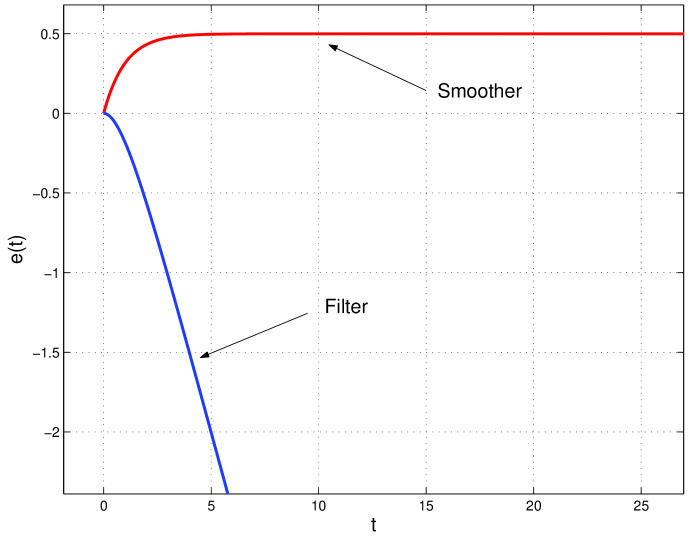
Figure 2: The steady-state error of the first order smoother and filter with the polynomial input $\displaystyle\frac{at^{2}}{2}$ $(n=1,\ m=1)$. The smoother develops constant steady-state error, while, the error in the filter is unbounded.

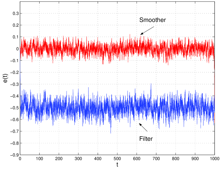
Figure 3: The estimation error in the first order smoother and filter in the offset case. No steady-state error develops in the smoother and the error variance in the smoother remains smaller.

4 Discussion and conclusions

The results reveal a significant robustness of the smoother to signals different than those, for which the smoother is optimal. In many applications in engineering practice, either there is no exact information about the signal, or the signal changes its characteristics with time. Thus, robustness of the system to the signal model is desirable. The results further indicate that the performance gap between smoothers and filters with respect to the criterion of mean square error increases as the difference between the incoming signal and the nominal signal increases.

The fact that a smoother, optimal for a $n$-th order signal, exhibits a steady-state error regime of a type $2n$ causal filter, without degradation in the error variance, is very appealing from the engineering point of view. This is due to the facts that in many applications lag estimation is possible and that linear smoothers are rather easy to implement, for example, by using approximate finite impulse response (FIR) non-causal filters. Utilizing smoothers to exploit their superior tracking properties may free the designer from the traditional trade-off that exists in causal filtering between steady-state error regime and error variance.

Steady-state errors also appear in nonlinear estimators, as shown in nonlinear filtering [18, 19]. An extension of the ideas demonstrated here to nonlinear smoothing will be given in a forthcoming paper.

References

• [1] Anderson, B.D.O. Fixed interval smoothing for nonlinear continuous time systems. J. Info. Control, 20:294–300, 1972.
• [2] Bellman, R., Kalba, R., and Middelton, D. Dynamic programming, sequential estimation and sequential detection processes. Proc. Nat. Acad. Sci.U.S.A., 47:338 341, 1961.
• [3] Bryson, A.B., and Ho, Y.C. Applied Optimal Control. John Wiley, New York, 1975.
• [4] Deuschel J.D., and Stroock, D.W. Large Deviations. Academic Press, 1989.
• [5] Dorf, R.C., and Bishop, R.H. Modern Control Systems, volume I. Addison Wesley, 1992.
• [6] Einicke, G.A. Asymptotic optimality of the minimum-variance fixed-interval smoother. IEEE Transactions on Signal Processing, 55 (4), pp.1543–1547 (2007).
• [7] Kailath, T., and Frost, P. An innovation approach to least-squares estimation part II: Linear smoothing in addative white noise. IEEE Trans. Auto. Contronl, AC-13:655–660, 1968.
• [8] Kalman, R.E., and Bucy, R.S. New results in linear filtering and prediction theory. Trans. AMSE, Ser. D., J. Basic Engng, 83:95–108, 1961.
• [9] Kirk D.E. Optimal Control Theory - an Introduction. Prentice-Hall, Inc., 1970.
• [10] Lee, R.C.K. Optimal Estimation Idetification and Control. M.I.T. Press, 1964.
• [11] Leondes, C.T., Peller, J.B., and Stear, E.B. Nonlinear smoothing theory. IEEE Trans. Sys. Sci. Cyb., SSC-6:63–71, 1970.
• [12] Rauch, H.E. Linear estimation of sampled stochastic processes with random parameters. Technical Report 2108, Stanford Electronics Labratory, Stanford University, California, 1962.
• [13] Rauch, H.E. Solutions to the linear smoothing problem. IEEE Tans. Auto. Control., AC-8:371–372, 1963.
• [14] Rauch, H.E., Tung, F., and Steibel, C.T. Maximum likelihood estimates of linear dynamic systems. AIAA J., 3:1445–1450, 1965.
• [15] Sage, A.P. Maximum a posteriori filtering and smoothing algorithms. Int. J. Control, 11:171–183, 1970.
• [16] Sage, A.P., and Ewing, W.S. On filtering and smoothing algorithms for nonlinear state estimation. Int. J. Control, 11:1–18, 1970.
• [17] Weaver, C.S. Estimating the output of a linear discrete system with Gaussian input. IEEE Trans. Auto. Control, AC-8:372–374, 1963.
• [18] Welti, A.L., and Bobrovsky, B.Z. Mean time to lose lock for a coherent second-order PN-code tracking loop-the singular perturbation approach. IEEE J. on Selected Areas in Comm., 8:809–18, 1990.
• [19] Welti, A.L., Bernhard, U.P., and Bobrovsky, B.Z. Third-order delay-locked loop: Mean time to lose lock and optimal parameters. IEEE Trans. on Comm., 43:2540–50, 1995.