Interatomic van der Waals potential in the presence of a magneto-electric sphere

Abstract

On the basis of a general formula obtained earlier via fourth-order perturbation theory within the framework of macroscopic quantum electrodynamics, the van der Waals potential between two neutral, unpolarized, ground-state atoms in the presence of a homogeneous, dispersing and absorbing magneto-electric sphere is studied. When the radius of the sphere becomes sufficiently large, the result asymptotically agrees with that for two atoms near a planar interface. In the opposite limit of a very small sphere, the sphere can effectively be regarded as being a third ground-state atom, and the nonadditive three-atom van der Waals potential is recovered. To illustrate the effect of a sphere of arbitrary radius, numerical results are presented for the triangular arrangement where the atoms are at equidistance from the sphere, and for the linear arrangement where the atoms and the sphere are aligned along a straight line. As demonstrated, the enhancement or reduction of the interaction potential in the presence of purely electric or magnetic spheres can be physically understood in terms of image charges.

I Introduction

Electromagnetic and material ground-state fluctuations are well known to produce observable effects such as dispersion forces between atoms, between atoms and bodies, or between bodies rev2 . The van der Waals (vdW) potential between two ground-state atoms in free space was first calculated by London for small interatomic separation (nonretarded limit), using perturbation theory to the leading (second) order Lon . In this limit, the result is an attractive potential proportional to $r^{-6}$, where $r$ denotes the interatomic distance. The (nonretarded) London potential was extended to arbitrary distances between the two atoms by Casimir and Polder CP , using fourth-order perturbation theory within the framework of full quantum electrodynamics (QED). In particular for large interatomic separation the potential was predicted to vary as $r^{-7}$. Recently, the closely related Casimir interaction between two magnetoelectric spheres has been studied by means of a scattering method Emig , where the inclusion of higher-order multipoles have been shown to lead to corrections of the Casimir–Polder result. In the three-atom case, a non-additive term prevents the potential from just being the sum of three pairwise contributions. This three-atom vdW potential was calculated first in the nonretarded limit by pursuing the perturbation calculation to the third order Ax , and then for arbitrary interatomic distances, by using sixth-order perturbation calculation Aub . Later on, a general formula for the non-additive $N$-atom vdW potential was derived by summing up the response of each atom to the quantized field caused by the other atoms Pow1 and by calculating the difference in the zero-point energy of the electromagnetic field of a large cavity with and without the atoms Pow2 .

The presence of macroscopic bodies modifies the fluctuation of the electromagnetic field, and consequently, the interatomic vdW interaction. A general formula expressing the vdW potential between two ground-state atoms in the presence of electrically polarizable bodies in terms of the Green tensor of the body-assisted electromagnetic field was first obtained by means of linear response theory Mc , an later by treating the effect of the bodies semiclassically Mah1 . An exact derivation of the formula based on fourth-order perturbation theory within the framework of macroscopic QED has been given recently h , where both electrically and magnetically polarizable bodies—referred to as magneto-electric bodies—are explicitly taken into account, and a generalization of the formula to the $N$-atom case has also been given BSW . The two-atom potential in the presence of arbitrary magnetoelectric bodies has recently been generalized to atoms having both electric and magnetic polarizabilities using linear response theory and was explicitly calculated for atoms embedded in a bulk medium Spag1 . Various special cases such as two atoms placed between two perfectly conducting plates Mah1 , in a bulk magneto-electric medium Mah2 ; Spag2 ; Sin ; h , near a perfectly reflecting plate h , and near a planar magneto-electric multilayer system h have been considered. Local-field corrections to the vdW potential that appear when the atoms are embedded in optically dense media have also been addressed agnes ; tomas .

On the experimental side, the vdW interaction between a single atom and a body has been explored by means of detecting the intensity of an atomic beam transmitted through a parallel-plate cavity suk ; direct force measurement using atomic-mirror techniques land ; moh ; measuring the intensity of a diffracted atomic beam from a transmission-grating gri ; making use of quantum reflection from a solid surface at nonretarded Druzhinina and retarded Pasquini1 ; Pasquini2 atom–surface separations; determining their effect on the collective oscillation frequency of the magnetically trapped atoms Obrecht . Observations of interatomic vdW interactions based on a determination of the scattering cross sections in the atomic collisions between two ground-state atomic beams chen , between an atomic beam and the atoms of a stationary target gas bru1 ; bru2 , and between a beam of ground-state atoms and a beam of excited atoms mar have been reported.

As already mentioned, the theoretical studies of medium-assisted interatomic vdW interactions have so far concentrated on bulk media and infinitely extended planar (multi-layer) bodies Here we shall consider the vdW interaction between two ground-state atoms located near a finite-size body, namely, a sphere. With recent progress in fabrication of metamaterials in mind, we allow for the sphere to exhibit both electric and magnetic properties. Note that the single-atom vdW potential in the presence of a sphere has been investigated earlier st1 .

The paper is organized as follows. The basic formulas for calculating the vdW potential between two atoms in the presence of an arbitrary arrangement of magneto-electric bodies are summarized in Sec. II. In Sec. III, the theory is applied to the case of a magneto-electric sphere, and the limiting cases of large and small sphere are considered. Detailed numerical results are presented in Sec. IV. Finally, the paper ends with a summary in Sec. V.

II Basic formulas

Consider two neutral, unpolarized, ground state atoms $A$ and $B$ with spherically symmetric polarizabilities in the presence of an arbitrary arrangement of dispersing and absorbing magneto-electric bodies. The total force acting on the atoms can be derived from the potential

$$U(\mathbf{r}_{A},\mathbf{r}_{B})=U_{A}(\mathbf{r}_{A})+U_{B}(\mathbf{r}_{B})+U_{AB}(\mathbf{r}_{A},\mathbf{r}_{B})$$ (1)

according to

$$\mathbf{F}_{A^{\prime}}(\mathbf{r}_{A^{\prime}})=-\bm{\nabla}_{\mathbf{r}_{A^{\prime}}}U(\mathbf{r}_{A},\mathbf{r}_{B}),$$ (2)

($A^{\prime}$ $\!=$ $\!A,$ $\!B$), where $U_{A^{\prime}}$ is the single-atom potential st1

$$U_{A^{\prime}}(\mathbf{r}_{A^{\prime}})=\frac{\hbar\mu_{0}}{2\pi}\int_{0}^{\infty}\mathrm{d}u\,u^{2}\alpha_{A^{\prime}}(iu)\mathrm{Tr}{\bm{G}}^{(1)}(\mathbf{r}_{A^{\prime}},\mathbf{r}_{A^{\prime}},iu),$$ (3)

and $U_{AB}$ is the two-atom interaction potential h

$$U_{AB}(\mathbf{r}_{A},\mathbf{r}_{B})=-\frac{\hbar\mu_{0}^{2}}{2\pi}\int_{0}^{\infty}\mathrm{d}u\,u^{4}\alpha_{A}(iu)\alpha_{B}(iu)\\ \times\mathrm{Tr}[{\bm{G}}(\mathbf{r}_{A},\mathbf{r}_{B},iu)\!\cdot\!{\bm{G}}(\mathbf{r}_{B},\mathbf{r}_{A},iu)].$$ (4)

In Eqs. (3) and (4), ${\alpha}_{A^{\prime}}$ is the (lowest-order) polarizability of the atom $A^{\prime}$

$$\alpha_{A^{\prime}}(\omega)=\lim_{\eta\rightarrow 0^{+}}\frac{2}{3\hbar}\sum_{k}\frac{\omega^{k0}_{A^{\prime}}|\mathbf{d}^{k0}_{A^{\prime}}|^{2}}{(\omega^{k0}_{A^{\prime}})^{2}-\omega^{2}-i\eta\omega}\,,$$ (5)

with $\omega^{k0}_{A^{\prime}}$ and $\mathbf{d}^{k0}_{A^{\prime}}$ being, respectively, the transition frequency and transition electric dipole moment between the $k$th excited state and the ground state of atom $A^{\prime}$, and $\bm{G}(\mathbf{r},\mathbf{r^{\prime}},\omega)$ is the classical Green tensor obeying the differential equation

$$\bm{\nabla}\times\frac{1}{\mu(\mathbf{r},\omega)}\bm{\nabla}\times\bm{G}(\mathbf{r},\mathbf{r^{\prime}},\omega)\\ -\frac{\omega^{2}}{c^{2}}\,\varepsilon(\mathbf{r},\omega)\bm{G}(\mathbf{r},\mathbf{r^{\prime}},\omega)=\bm{\delta}(\mathbf{r}-\mathbf{r^{\prime}})$$ (6)

together with the boundary condition at infinity. Note that the electromagnetic and geometric properties of the bodies are fully incorporated in the Green tensor via the space- and frequency-dependent permittivity $\varepsilon(\mathbf{r},\omega)$ and permeability $\mu(\mathbf{r},\omega)$. When $\mathbf{r}$ and $\mathbf{r}^{\prime}$ denote two positions in free space which can be connected without crossing a body, then the Green tensor can be decomposed as

$$\bm{G}(\mathbf{r},\mathbf{r}^{\prime},\omega)=\bm{G}^{(0)}(\mathbf{r},\mathbf{r}^{\prime},\omega)+\bm{G}^{(1)}(\mathbf{r},\mathbf{r}^{\prime},\omega),$$ (7)

where $\bm{G}^{(0)}$ is the free-space Green tensor which is obtained from Eq. (6) by letting $\varepsilon(\mathbf{r},\omega)$ $\!=$ $\!\mu(\mathbf{r},\omega)$ $\!=$ $\!1$, and $\bm{G}^{(1)}$ is the scattering part of the Green tensor.

In what follows we concentrate on the atom–atom interaction potential $U_{AB}$ in the presence of a sphere (for the single-atom potentials $U_{A}(\mathbf{r}_{A})$ and $U_{B}(\mathbf{r}_{B})$, see Ref. st1 ). According to Eq. (7), the potential $U_{AB}(\mathbf{r}_{A},\mathbf{r}_{B})$ can be cast in the form

$$U_{AB}(\mathbf{r}_{A},\mathbf{r}_{B})=U^{(0)}(\mathbf{r}_{A},\mathbf{r}_{B})+U^{(b)}(\mathbf{r}_{A},\mathbf{r}_{B}),$$ (8)

where

$$U^{(0)}(\mathbf{r}_{A},\mathbf{r}_{B})=-\frac{\hbar\mu_{0}^{2}}{2\pi}\int_{0}^{\infty}{\mathrm{d}}u\,u^{4}\alpha_{A}(iu)\alpha_{B}(iu)\\ \times\mathrm{Tr}\!\left[\bm{G}^{(0)}(\mathbf{r}_{A},\mathbf{r}_{B},iu)\cdot\bm{G}^{(0)}(\mathbf{r}_{B},\mathbf{r}_{A},iu)\right]$$ (9)

is the potential observed in the case when the two atoms are in free space, and $U^{(b)}$ is the body-induced part which can be written as

$$U^{(b)}(\mathbf{r}_{A},\mathbf{r}_{B})=U^{(1)}(\mathbf{r}_{A},\mathbf{r}_{B})+U^{(2)}(\mathbf{r}_{A},\mathbf{r}_{B}),$$ (10)

where

$$U^{(1)}(\mathbf{r}_{A},\mathbf{r}_{B})=-\frac{\hbar\mu_{0}^{2}}{\pi}\int_{0}^{\infty}{\mathrm{d}}u\,u^{4}\alpha_{A}(iu)\alpha_{B}(iu)\\ \times\mathrm{Tr}\!\left[\bm{G}^{(0)}(\mathbf{r}_{A},\mathbf{r}_{B},iu)\cdot\bm{G}^{(1)}(\mathbf{r}_{B}\mathbf{r}_{A},iu)\right]$$ (11)

is the contribution due to the cross term of the free-space part and the scattering parts of the Green tensor, and

$$U^{(2)}(\mathbf{r}_{A},\mathbf{r}_{B})=-\frac{\hbar\mu_{0}^{2}}{2\pi}\int_{0}^{\infty}{\mathrm{d}}u\,u^{4}\alpha_{A}(iu)\alpha_{B}(iu)\\ \times\mathrm{Tr}\!\left[\bm{G}^{(1)}(\mathbf{r}_{A},\mathbf{r}_{B},iu)\cdot\bm{G}^{(1)}(\mathbf{r}_{B},\mathbf{r}_{A},iu)\right]$$ (12)

is the scattering-part contribution.

The free-space Green tensor reads (see, e.g., Ref. rev )

$${\bm{G}}^{(0)}(\mathbf{r}_{A},\mathbf{r}_{B},\omega)\\ =-\frac{c^{2}}{4\pi\omega^{2}l^{3}}\left[f(-il\omega/c)\bm{I}-g(-il\omega/c)\frac{\mathbf{l}\mathbf{l}}{l^{2}}\right]e^{il\omega/c}$$ (13)

($\mathbf{r}_{A}$ $\!\neq$ $\!\mathbf{r}_{B}$), where $\bm{I}$ denotes the unit tensor, $\mathbf{l}$ $\!=$ $\!\mathbf{r}_{B}$ $\!-$ $\!\mathbf{r}_{A}$, $l$ $\!=$ $\!|\mathbf{l}|$, and

$$f(x)=1+x+x^{2},$$ (14)

$$g(x)=3+3x+x^{2}.$$ (15)

By substituting Eq. (13) together with Eqs. (14) and (15) into Eq. (9), the well known Casimir–Polder interaction potential between two ground-state atoms in free space are obtained,

$$U^{(0)}(\mathbf{r}_{A},\mathbf{r}_{B})=-\frac{\hbar}{16\pi^{3}\varepsilon_{0}^{2}l^{6}}\int_{0}^{\infty}\!\!{\rm d}u\alpha_{A}(iu)\alpha_{B}(iu)e^{-2lu/c}\\ \times\left[3+\frac{6lu}{c}+\frac{5l^{2}u^{2}}{c^{2}}+\frac{2l^{3}u^{3}}{c^{3}}+\frac{l^{4}u^{4}}{c^{4}}\right].$$ (16)

Needless to say that the scattering part of the Green tensor depends on the specific arrangement of the bodies under consideration.

III Two atoms in the presence of a magneto-electric sphere

Let us consider two atoms $A$ and $B$ in the presence of a homogeneous magneto-electric sphere of permittivity $\varepsilon(\omega)$, permeability $\mu(\omega)$, and radius $R$. Choosing the coordinate system such that its origin coincides with the center of the sphere, we may represent the scattering part of the Green tensor as le-wei

$${\bm{G}}^{(1)}(\mathbf{r}_{A},\mathbf{r}_{B},\omega)\!=\!\frac{i\omega}{4\pi c}\sum_{n=1}^{\infty}\frac{2n\!+\!1}{n(n\!+\!1)}\sum_{m=0}^{n}\frac{(n\!-\!m)!}{(n\!+\!m)!}(2\!-\!\delta_{0m})\\ \times\sum_{p=\pm 1}\left[B_{n}^{M}(\omega)\mathbf{M}_{nm,p}(\mathbf{r}_{A},\omega/c)\mathbf{M}_{nm,p}(\mathbf{r}_{B},\omega/c)\right.\\ \left.+B_{n}^{N}(\omega)\mathbf{N}_{nm,p}(\mathbf{r}_{A},\omega/c)\mathbf{N}_{nm,p}(\mathbf{r}_{B},\omega/c)\right],$$ (17)

where $\mathbf{M}_{nm,p}(\mathbf{r},q)$ and $\mathbf{N}_{nm,p}(\mathbf{r},q)$ are even ($p$ $\!=$ $\!+1$) and odd ($p$ $\!=$ $\!-1$) spherical wave vector functions. In spherical coordinates, they can be expressed in terms of spherical Hankel functions of the first kind, $h^{(1)}_{n}(x)$, and Legendre functions, $P_{n}^{m}(x)$, as follows:

$$\mathbf{M}_{nm,\pm 1}(\mathbf{r},q)=\mp\frac{m}{\sin\theta}\,h^{(1)}_{n}(qr)P_{n}^{m}(\cos\theta)\genfrac{}{}{0.0pt}{}{\sin}{\cos}(m\phi)\mathbf{e}_{\theta}\\ -h^{(1)}_{n}(qr)\frac{\mathrm{d}P_{n}^{m}(\cos\theta)}{\mathrm{d}\theta}\,\genfrac{}{}{0.0pt}{}{\cos}{\sin}(m\phi)\mathbf{e}_{\phi},$$ (18)

$$\mathbf{N}_{nm,\pm 1}(\mathbf{r},q)=\frac{n(n+1)}{qr}\,h^{(1)}_{n}(qr)P_{n}^{m}(\cos\theta)\genfrac{}{}{0.0pt}{}{\cos}{\sin}(m\phi)\mathbf{e}_{r}\\ +\frac{1}{qr}\frac{\mathrm{d}[rh^{(1)}_{n}(qr)]}{\mathrm{d}r}\left[\frac{\mathrm{d}P_{n}^{m}(\cos\theta)}{\mathrm{d}\theta}\,\genfrac{}{}{0.0pt}{}{\cos}{\sin}(m\phi)\mathbf{e}_{\theta}\right.\\ \left.\mp\frac{m}{\sin\theta}\,P_{n}^{m}(\cos\theta)\genfrac{}{}{0.0pt}{}{\sin}{\cos}(m\phi)\mathbf{e}_{\phi}\right],$$ (19)

with $\mathbf{e}_{r}$, $\mathbf{e}_{\theta}$, and $\mathbf{e}_{\phi}$ being the mutually orthogonal unit vectors pointing in the directions of radial distance $r$, polar angle $\theta$, and azimuthal angle $\phi$, respectively (inset in Fig. 1). The coefficients $B_{n}^{M}(\omega)$ and $B_{n}^{N}(\omega)$ in Eq. (17) read

$$B_{n}^{M}(\omega)=-\frac{\mu(\omega)[z_{0}j_{n}(z_{0})]^{\prime}j_{n}(z_{1})\!-\![z_{1}j_{n}(z_{1})]^{\prime}j_{n}(z_{0})}{\mu(\omega)[z_{0}h^{(1)}_{n}(z_{0})]^{\prime}j_{n}(z_{1})\!-\![z_{1}j_{n}(z_{1})]^{\prime}h^{(1)}_{n}(z_{0})}\,,$$ (20)

$$B_{n}^{N}(\omega)=-\frac{\varepsilon(\omega)[z_{0}j_{n}(z_{0})]^{\prime}j_{n}(z_{1})-[z_{1}j_{n}(z_{1})]^{\prime}j_{n}(z_{0})}{\varepsilon(\omega)[z_{0}h^{(1)}_{n}(z_{0})]^{\prime}j_{n}(z_{1})-[z_{1}j_{n}(z_{1})]^{\prime}h^{(1)}_{n}(z_{0})},$$ (21)

where $j_{n}(z)$ is the spherical Bessel function of the first kind, $z_{0}$ $\!=$ $\!kR$ ($k$ $\!=$ $\!\omega/c$), $z_{1}$ $\!=$ $\!\sqrt{\varepsilon(\omega)\mu(\omega)}z_{0}$ $\!=$ $\!n(\omega)z_{0}$, and the prime denotes differentiation with respect to the respective argument.

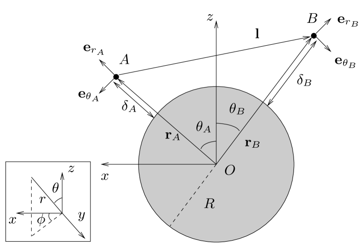
Figure 1: Two atoms $A$ and $B$ in the presence of a sphere

Without loss of generality, we assume that the two atoms are located in the $xz$-plane (Fig. 1),

$$\mathbf{r}_{A}=(r_{A},\theta_{A},0),\quad\mathbf{r}_{B}=(r_{B},\theta_{B},\pi).$$ (22)

Substituting Eqs. (18) and (19) [together with Eq. (22)] into Eq. (17), and performing the summations over $m$ and $p$, we derive (Appendix A)

$${\bm{G}}^{(1)}(\mathbf{r}_{A},\mathbf{r}_{B},iu)=\sum_{ij}G_{ij}^{(1)}(\mathbf{r}_{A},\mathbf{r}_{B},iu)\mathbf{e}_{i_{A}}\mathbf{e}_{j_{B}}$$ (23)

($i,j$ $\!=$ $\!r,\theta,\phi$), with the nonzero elements being

$$G^{(1)}_{rr}(\mathbf{r}_{A},\mathbf{r}_{B},\omega)=\frac{ic}{4\pi\omega r_{A}r_{B}}\\ \times\sum_{n=1}^{\infty}n(n\!+\!1)(2n\!+\!1)B_{n}^{N}(\omega)P_{n}(\gamma)Q_{n}^{(1)},$$ (24)

$$G^{(1)}_{\genfrac{}{}{0.0pt}{}{r\theta}{\theta r}}(\mathbf{r}_{A},\mathbf{r}_{B},\omega)\\ =\frac{-ic\sin\Theta}{4\pi\omega r_{A}r_{B}}\sum_{n=1}^{\infty}(2n\!+\!1)B_{n}^{N}(\omega)P_{n}^{\prime}(\gamma)\genfrac{}{}{0.0pt}{}{Q_{n}^{(2)}}{Q_{n}^{(3)}},$$ (25)

$$G^{(1)}_{\genfrac{}{}{0.0pt}{}{\theta\theta}{\phi\phi}}(\mathbf{r}_{A},\mathbf{r}_{B},\omega)=-\frac{i\omega}{4\pi c}\sum_{n=1}^{\infty}\frac{2n+1}{n(n+1)}\\ \times\left[B_{n}^{M}(\omega)\genfrac{}{}{0.0pt}{}{P^{\prime}_{n}(\gamma)}{F_{n}(\gamma)}Q_{n}^{(1)}+\frac{c^{2}B_{n}^{N}(\omega)}{\omega^{2}r_{A}r_{B}}\genfrac{}{}{0.0pt}{}{F_{n}(\gamma)}{P_{n}^{\prime}(\gamma)}Q_{n}^{(4)}\right],$$ (26)

where $\Theta$ $\!=$ $\!\theta_{A}$ $\!+$ $\!\theta_{B}$, $\gamma$ $\!=$ $\!\cos\Theta$, and

$$Q^{(1)}_{n}=h_{n}^{(1)}(kr_{A})h_{n}^{(1)}(kr_{B}),$$ (27)

$$Q_{n}^{(2)}=h_{n}^{(1)}(kr_{A})[zh_{n}^{(1)}(z)]^{\prime}_{z=kr_{B}},$$ (28)

$$Q_{n}^{(3)}=h_{n}^{(1)}(kr_{B})[yh_{n}^{(1)}(y)]^{\prime}_{y=kr_{A}},$$ (29)

$$Q_{n}^{(4)}=[yh_{n}^{(1)}(y)]^{\prime}_{y=kr_{A}}[zh_{n}^{(1)}(z)]^{\prime}_{z=kr_{B}},$$ (30)

$$F_{n}(x)=n(n+1)P_{n}(x)-xP_{n}^{\prime}(x).$$ (31)

To facilitate further evaluations, it is convenient to represent the free-space Green tensor (13) in the same spherical coordinate system as the scattering part, so that its nonzero elements read

$$G_{rr}^{(0)}(\mathbf{r}_{A},\mathbf{r}_{B},iu)=\frac{c^{2}}{4\pi u^{2}l^{5}}\big{[}l^{2}f(\xi)\cos\Theta-g(\xi)l_{A}l_{B}\big{]}e^{-\xi},$$ (32)

$$G_{r\theta(\theta r)}^{(0)}(\mathbf{r}_{A},\mathbf{r}_{B},iu)=\frac{-c^{2}\sin\Theta}{4\pi u^{2}l^{5}}\\ \times\left[l^{2}f(\xi)\pm g(\xi)r_{A(B)}l_{A(B)}\right]e^{-\xi},$$ (33)

$$G_{\theta\theta}^{(0)}(\mathbf{r}_{A},\mathbf{r}_{B},iu)=\frac{-c^{2}}{4\pi u^{2}l^{5}}\\ \times\left[l^{2}f(\xi)\cos\Theta-g(\xi)r_{A}r_{B}\sin^{2}\Theta\right]e^{-\xi},$$ (34)

$$G_{\phi\phi}^{(0)}(\mathbf{r}_{A},\mathbf{r}_{B},iu)=-\frac{c^{2}}{4\pi u^{2}l^{3}}\,f(\xi)e^{-\xi},$$ (35)

where $\xi$ $\!=$ $\!lu/c$, $l_{A}$ $\!=$ $\!r_{B}\cos\Theta$ $\!-$ $\!r_{A}$ and $l_{B}$ $\!=$ $\!r_{B}$ $\!-r_{A}\cos\Theta$.

Recalling Eqs. (10)–(12), we may write the body-induced part of the interaction potential as

$$U^{(b)}(\mathbf{r}_{A},\mathbf{r}_{B})=\sum_{i,j}\left[U^{(1)}_{ij}(\mathbf{r}_{A},\mathbf{r}_{B})+U^{(2)}_{ij}(\mathbf{r}_{A},\mathbf{r}_{B})\right],$$ (36)

where

$$U^{(1)}_{ij}(\mathbf{r}_{A},\mathbf{r}_{B})=-\frac{\hbar\mu_{0}^{2}}{\pi}\int_{0}^{\infty}\mathrm{d}u\,u^{4}\alpha_{A}(iu)\alpha_{B}(iu)\\ \times G^{(0)}_{ij}(\mathbf{r}_{A},\mathbf{r}_{B},iu)G^{(1)}_{ij}(\mathbf{r}_{A},\mathbf{r}_{B},iu),$$ (37)

$$U^{(2)}_{ij}(\mathbf{r}_{A},\mathbf{r}_{B})=-\frac{\hbar\mu_{0}^{2}}{2\pi}\int_{0}^{\infty}\mathrm{d}u\,u^{4}\alpha_{A}(iu)\alpha_{B}(iu)\\ \times\left[G^{(1)}_{ij}(\mathbf{r}_{A},\mathbf{r}_{B},iu)\right]^{2},$$ (38)

with $G^{(1)}_{ij}(\mathbf{r}_{A},\mathbf{r}_{B},iu)$ and $G^{(0)}_{ij}(\mathbf{r}_{A},\mathbf{r}_{B},iu)$ according to Eqs. (24)–(26) and Eqs. (32)–(35), respectively (see Appendix B). Further evaluation of $U^{(b)}(\mathrm{r}_{A},\mathrm{r}_{B})$ requires numerical methods in general. Before doing so, let us consider the limiting cases of large and small spheres.

III.1 Large sphere

The limiting case of a large sphere may be defined by the requirement that

$$\delta_{A^{\prime}}\equiv r_{A^{\prime}}-R\ll R\quad(A^{\prime}=A,B)$$ (39)

and

$$l\ll R\quad\leadsto\quad\Theta=\theta_{A}+\theta_{B}\ll 1$$ (40)

(cf. Fig. 1). In this limit, Eq. (36) leads to (Appendix C)

$$U^{(b)}(\mathbf{r}_{A},\mathbf{r}_{B})=\\ \frac{\hbar}{16\pi^{3}\varepsilon_{0}^{2}l^{5}l_{+}^{5}}\biggl{\{}\left[4X^{4}-2\delta_{-}^{2}\delta_{+}^{2}+X^{2}(\delta_{-}^{2}+\delta_{+}^{2})\right]I_{01}\\ +\frac{l_{+}^{2}}{4R}\left[3(l_{+}^{3}-\delta_{+}^{3})-\delta_{+}(\delta_{-}^{2}+4X^{2})\right]I_{11}\\ -\frac{3l^{5}}{l_{+}}\left(I_{02}+\frac{l_{+}}{4R}I_{12}\right)\biggr{\}},$$ (41)

where $X$ $\!=$ $\!-R\Theta$, $\delta_{\pm}$ $\!=$ $\!\delta_{B}$ $\!\pm$ $\!\delta_{A}$, $l_{+}$ $\!=$ $\!(X^{2}$ $\!+$ $\!\delta_{+}^{2})^{1/2}$, and

$$I_{kl}=\int_{0}^{\infty}\mathrm{d}u\,\alpha_{A}(iu)\alpha_{B}(iu)\\ \times\left[26+\varepsilon(iu)\mu(iu)R^{2}u^{2}/c^{2}\right]^{k}\left[\frac{\varepsilon(iu)-1}{\varepsilon(iu)+1}\right]^{l}.$$ (42)

Note that the case of a purely electrically polarizable sphere can be simply obtained by setting $\mu(iu)$ $\!=$ $\!1$ in Eq. (41).

For a purely magnetically polarizable sphere [$\varepsilon(iu)$ $\!=$ $\!1$] Eq. (36) leads, under the conditions (39) and (40), to (Appendix C)

$$U^{(b)}(\mathbf{r}_{A},\mathbf{r}_{B})=\frac{\hbar\left[\delta_{-}^{2}-2X^{2}+3\delta_{+}(l_{+}-\delta_{+})\right]}{64\pi^{3}\varepsilon_{0}^{2}c^{2}l^{5}l_{+}}\\ \times\int_{0}^{\infty}\mathrm{d}u\,u^{2}\alpha_{A}(iu)\alpha_{B}(iu)\frac{\left[\mu(iu)-1][\mu(iu)-3\right]}{\mu(iu)+1}.$$ (43)

As expected, Eqs. (41) and (43) are in agreement with those found for a half-space ($l_{+}/R$ $\!\rightarrow$ $\!0$) h .

III.2 Small spheres

In the opposite limit of a small sphere, where

$$R\ll r_{A^{\prime}}\quad(A^{\prime}=A,B),$$ (44)

Eq. (36) leads to (Appendix C)

$$U^{(b)}(\mathbf{r}_{A},\mathbf{r}_{B})\\ =\frac{\hbar}{64\pi^{4}\varepsilon_{0}^{3}r_{A}^{3}r_{B}^{3}l^{3}}\int_{0}^{\infty}\mathrm{d}u\alpha_{A}(iu)\alpha_{B}(iu)e^{-(r_{A}+r_{B}+l)u/c}\\ \times\!\biggl{\{}\alpha_{\mathrm{sp}}(iu)\biggl{[}f(\xi)\big{\{}g(b)\big{[}2(1\!+\!a)\!\!-\!g(a)\sin^{2}\Theta\big{]}\!+\!2a^{2}f(b)\big{\}}\\ +\frac{g(\xi)}{l^{2}}\big{\{}\big{[}(2l^{2}\!-\!r_{A}r_{B}\cos\Theta)f(a)f(b)\!+\!2a^{2}f(b)r_{A}l_{A}\\ -\!2b^{2}f(a)r_{B}l_{B}\big{]}\sin^{2}\Theta\!-\!4(1\!+\!a)(1\!+\!b)l_{A}l_{B}\cos\Theta\big{\}}\biggr{]}\\ +\frac{ab}{c^{2}}(1\!+\!a)(1\!+\!b)\beta_{\mathrm{sp}}(iu)\biggl{[}g(\xi)\frac{r_{A}r_{B}}{l^{2}}\sin^{2}\Theta\\ -2f(\xi)\cos\Theta\biggr{]}\biggr{\}}$$ (45)

($a$ $\!=$ $\!r_{A}u/c$, $b$ $\!=$ $\!r_{B}u/c$), where

$$\alpha_{\mathrm{sp}}(\omega)=4\pi\varepsilon_{0}R^{3}\,\frac{\varepsilon(\omega)-1}{\varepsilon(\omega)+2},$$ (46)

$$\beta_{\mathrm{sp}}(\omega)=\frac{4\pi R^{3}}{\mu_{0}}\,\frac{\mu(\omega)-1}{\mu(\omega)+2}.$$ (47)

Let us consider a sphere to which the Clausius–Mossotti relation applies, so that

$$\frac{\varepsilon(\omega)-1}{\varepsilon(\omega)+2}=\frac{1}{3\varepsilon_{0}}\sum_{k}n_{k}\alpha_{k}(\omega),$$ (48)

with $n_{k}$ and $\alpha_{k}(\omega)$, respectively, being the number density and the polarizability of the atoms of type $k$. In this case, Eq. (46) can be rewritten as

$$\alpha_{sp}(\omega)=\sum_{k}n_{k}\alpha_{k}(\omega),$$ (49)

where $N_{k}$ is the number of atoms of type $k$ of the sphere. Accordingly, the magnetic analog of Eq. (49) is

$$\beta_{sp}(\omega)=\sum_{k}n_{k}\beta_{k}(\omega),$$ (50)

with $\beta_{k}(\omega)$ being the magnetizability of the atoms of type $k$. Hence, we may replace in Eq. (45) the sphere parameters $\alpha_{\mathrm{sp}}(iu)$ and $\beta_{\mathrm{sp}}(iu)$, respectively, with the electric and magnetic polarizability of a single atom [say $\alpha_{k}(iu)$ and $\beta_{k}(iu)$], to obtain the nonadditive interaction potential of three atoms, two of which being purely electrically polarizable whereas the third atom being simultaneously electrically and magnetically polarizable. Indeed, after a straightforward but lengthy calculation, it can be shown that in the case of a purely electrically polarizable sphere, Eq. (45) [$\beta_{\mathrm{sp}}(iu)$ $\!=$ $\!0$] leads to the interaction potential between three electrically polarizable atoms, as derived in Refs. Ax ; Pow1 ; Pow2 ; Riz .

In the retarded limit where $l$,$r_{A}$,$r_{B}$ $\!\gg$ $\!c/\omega_{\mathrm{min}}$ ($\omega_{\mathrm{min}}$ denoting the minimum frequency among the relevant atomic and medium transition frequencies), due to the presence of the exponential term in the integral in Eq. (45), only small values of $u$ significantly contribute to the integral. Therefore, the electric and magnetic polarizabilities can be approximately replaced with their static values. After performing the remaining integral and expressing all the geometric parameters in terms of $r_{A}$, $r_{B}$, and $l$, we arrive at

$$U^{(b)}(\mathbf{r}_{A},\mathbf{r}_{B})=\frac{\hbar c\alpha_{A}(0)\alpha_{B}(0)}{32\pi^{4}\varepsilon_{0}^{3}r_{A}^{5}r_{B}^{5}l^{5}(r_{A}+r_{B}+l)^{7}}\\ \times\biggl{[}\alpha_{\mathrm{sp}}(0)\bigl{\{}\mathcal{S}[h_{1}(r_{A},r_{B},l)]+\mathcal{S}[h_{1}(r_{B},l,r_{A})]\\ +\mathcal{S}[h_{1}(l,r_{A},r_{B})]\bigr{\}}+\frac{r_{A}^{2}r_{B}^{2}}{c^{2}}\beta_{\mathrm{sp}}(0)\mathcal{S}[h_{2}(r_{A},r_{B},l)]\biggr{]},$$ (51)

where

$$h_{1}(x,y,z)=3x^{6}y^{2}(y\!-\!x)(x\!+\!y\!+\!7z)(x^{2}\!+\!7xy\!+\!11y^{2})\\ -x^{4}y^{2}z^{2}(53x^{4}+280x^{3}y-137x^{2}y^{2}\\ -329xy^{3}-623xy^{2}z-192y^{2}z^{2}),$$ (52)

$$h_{2}(x,y,z)=3x^{4}(y\!-\!x)(x\!+\!y\!+\!7z)(x^{2}\!+\!7xy\!+\!11y^{2})\\ -\!2x^{3}z^{2}(x\!+\!y)(26x^{2}\!+\!93xy\!-\!133y^{2})\!-\!7x^{2}z^{5}(3x\!-\!2y)\\ -\!14x^{3}z^{3}(2x^{2}\!-\!3xy\!-\!13y^{2})\!-\!x^{3}z^{4}(17x\!+\!161y)\\ +\!2xz^{6}(31x\!+\!105y)\!+\!5z^{7}(14x\!+\!z),$$ (53)

and $\mathcal{S}[f(x,y,z)]$ $\!=$ $f(x,y,z)$ $\!+$ $\!f(y,x,z)$.

In the nonretarded limit where $l$,$r_{A}$,$r_{B}$ $\!\ll$ $\!c/[n(0)\omega_{\mathrm{max}}]$ ($\omega_{\mathrm{max}}$ denoting the maximum frequency among the relevant atomic and medium transition frequencies), the leading contribution to the integral in Eq. (45) comes from the region where $e^{-(r_{A}+r_{B}+l)u/c}$ $\!\simeq$ $\!1$, so Eq. (45) reduces to

$$U^{(b)}(\mathbf{r}_{A},\mathbf{r}_{B})=\frac{3\hbar}{64\pi^{4}\varepsilon_{0}^{3}r_{A}^{3}r_{B}^{3}l^{3}}\\ \times\left\{\left[1\!-\!\frac{1}{l^{2}}(4l_{A}l_{B}\!+\!r_{A}r_{B}\sin^{2}\Theta)\cos\Theta+\!\cos^{2}\Theta\!\right]J_{1}\right.\\ \left.+\frac{r_{A}r_{B}}{c^{4}}\left(\frac{r_{A}r_{B}}{l^{2}}\sin^{2}\Theta\!-\!\frac{2}{3}\cos\Theta\right)J_{2}\right\},$$ (54)

where

$$J_{1}=\int_{0}^{\infty}\mathrm{d}u\,\alpha_{A}(iu)\alpha_{B}(iu)\alpha_{\mathrm{sp}}(iu),$$ (55)

$$J_{2}=\int_{0}^{\infty}\mathrm{d}u\,u^{2}\alpha_{A}(iu)\alpha_{B}(iu)\beta_{\mathrm{sp}}(iu).$$ (56)

In particular, in the case of a purely electrically polarizable sphere ($J_{2}$ $\!=$ $\!0$), Eq. (54) can be written in a very symmetric form. For this purpose we introduce the unit vectors ${\bm{a}}$, ${\bm{b}}$, and ${\bm{c}}$ pointing in the directions of $\mathbf{r}_{A}$, $\mathbf{l}$, and $-\mathbf{r}_{B}$, respectively (see Fig. 2). Noting that $l_{A}$ and $l_{B}$ defined below Eq. (35) are the components of the vector $\mathbf{l}$ in the directions of $\mathbf{r}_{A}$ and $\mathbf{r}_{B}$ and can thus be written as $l({\bm{a}}\!\cdot\!{\bm{b}})$ and $-l({\bm{b}}\!\cdot\!{\bm{c}})$, respectively, we see that

$$-\frac{1}{l^{2}}(4l_{A}l_{B}\!+\!r_{A}r_{B}\sin^{2}\Theta)+\!\cos\Theta\!=\!3({\bm{a}}\!\cdot\!{\bm{b}})({\bm{b}}\!\cdot\!{\bm{c}})$$ (57)

and can rewrite Eq. (54) as

$$U^{(b)}(\mathbf{r}_{A},\mathbf{r}_{B})=\frac{3\hbar}{64\pi^{4}\varepsilon_{0}^{3}r_{A}^{3}r_{B}^{3}l^{3}}\left[1-3({\bm{a}}\!\cdot\!{\bm{b}})({\bm{b}}\!\cdot\!{\bm{c}})({\bm{c}}\!\cdot\!{\bm{a}})\right]J_{1}.$$ (58)

If $\alpha_{sp}(iu)$ in Eq. (55) is again identified with the the electric polarizability of a single atom, Eq. (58) is nothing but the formula for the nonretarded three-atom interaction potential, which was first given by Axilrod and Teller Ax .

Figure 2: The triangle formed by the two atoms (at corners $A$ and $B$) and the sphere (at the corner $C$) in the small-sphere limit. It is seen that the vector products ${\bm{a}}\!\cdot\!{\bm{b}}$, ${\bm{b}}\!\cdot\!{\bm{c}}$ and ${\bm{c}}\!\cdot\!{\bm{a}}$ in the Axilrod and Teller’s formula Ax are equal to $-\cos\alpha$, $-\cos\beta$, and $-\cos\Theta$, respectively.

IV Numerical results

The effect of a medium-sized magneto-electric sphere on the mutual vdW interaction of two identical two-level atoms is illustrated in Figs. 3 and 4 showing the ratio $U_{AB}$ $/U^{(0)}$ [cf. Eq. (8)]. The results have been found by exact numerical evaluation of Eq. (36) together with Eqs. (72)–(78), where the permittivity and permeability of the sphere have been described by single-resonance Drude–Lorentz models,

$$\varepsilon(\omega)=1+\frac{\omega_{{\rm P}e}}{\omega_{{\rm T}e}^{2}-\omega^{2}-i\gamma_{e}\omega},$$ (59)

$$\mu(\omega)=1+\frac{\omega_{{\rm P}m}}{\omega_{{\rm T}m}^{2}-\omega^{2}-i\gamma_{m}\omega}.$$ (60)

Figure 3: The mutual vdW potential of two identical two-level atoms in a triangular configuration with (a) a purely electrically polarizable sphere with $\omega_{\mathrm{P}e}/\omega_{10}$ $\!=$ $\!3$, $\omega_{\mathrm{T}e}/\omega_{10}$ $\!=$ $\!1$, and $\gamma_{e}/\omega_{10}$ $\!=$ $\!0.001$ and (b) a purely magnetically polarizable sphere with $\omega_{\mathrm{P}m}/\omega_{10}$ $\!=$ $\!3$, $\omega_{\mathrm{T}m}/\omega_{10}$ $\!=$ $\!1$, and $\gamma_{m}/\omega_{10}=0.001$ is shown as a function of the atom–atom angular separation $\Theta$ ($\omega_{10}$ is the atomic transition frequency). The sphere radius is $R$ $\!=$ $\!c/\omega_{10}$ and the distances between the atoms and the center of the sphere are $r_{A}$ $\!=$ $\!r_{B}$ $\!=$ $\!1.03\,c/\omega_{10}$ (solid line), $1.3\,c/\omega_{10}$ (dashed line), and $2\,c/\omega_{10}$ (dotted line). $U^{(0)}$ is the potential observed in free space.

Figure 4: The mutual vdW potential of two identical two-level atoms in a linear configuration with (a) a purely electrically polarizable sphere and (b) a purely magnetically polarizable sphere is shown as a function of the interatomic distance $l$. Atom $A$ is held at a fixed position between atom $B$ and the sphere center with $r_{A}\!$ $\!=$ $\!1.03\,c/\omega_{10}$ (solid line), $1.1\,c/\omega_{10}$ (dashed line), and $1.3\,c/\omega_{10}$ (dotted line). All other parameters are the same as in Fig. 3.

In Fig. 3, a configuration is considered where the two atoms are positioned at equal distances from the sphere, $r_{A}$ $\!=$ $\!r_{B}$, briefly referred to as triangular configuration, and $U_{AB}/U^{(0)}$ is shown as a function of the angular separation $\Theta$ for three different values of the atom–sphere separation. For a purely electrically polarizable sphere [Fig. 3(a)], depending on the separation angle between the atoms, a (compared to the free-space case) relative reduction or enhancement of the vdW potential is possible, while for a purely magnetically polarizable sphere [Fig. 3(b)], the potential is typically reduced [note that for very small angular separations, a slight enhancement is possible, as can be seen from the inset in Fig. 3(b)], and the reduction increases with the angular separation. In both cases, the sphere-induced modification is strongest when the atoms are at opposite sides of the sphere ($\Theta$ $\!=$ $\!\pi$). Note that for small atom–sphere separations (solid curves) and small angular separations, the potential qualitatively agrees with the potential obtained for two atoms placed in parallel alignment near a semi-infinite half space h , as expected from the results in Sec. III.1.

In Fig. 4, a configuration is considered where the two atoms and the sphere center are aligned on a straight line, briefly referred to as linear configuration, and $U_{AB}/U^{(0)}$ is shown as a function of the interatomic distance for three different values of the position $r_{A}$ of atom $A$ which is positioned between the sphere and atom $B$. Unless both atoms are very close to the sphere, the sphere gives always rise to a (compared to the free-space case) relative enhancement of the vdW potential between the atoms; only for very small atom–sphere separations the potential can be reduced if the sphere is purely magnetically polarizable [inset in Fig. 4(b)]. Figure 4(a) shows that in the presence of a purely electrically polarizable sphere the relative enhancement of the potential increases with the interatomic separation $l$ and approaches a limit for larger interatomic separations, which depends on the separation distance between atom $A$ and the sphere. From Fig. 4(b) it is seen that in the presence of a purely magnetically polarizable sphere the relative enhancement of the potential increases with the interatomic separation $l$, reaches a maximum, and decreases with a further increase of $l$. In agreement with the results of Sec. III.1, the potential observed for small atom sphere separations (solid curves) and small interatomic separations qualitatively agrees with the potential obtained for two atoms placed in vertical alignment near a semi-infinite half space h .

Many features of the vdW potential observed in Figs. 3 and 4 can be subject to a physical interpretation via the method of image charges (the same approach as has been used for a planar geometry Ref. h ). Although being strictly valid only for sufficiently small atom–atom and atom–surface distances (such that retardation is negligible) and being most easily applicable in the perfect conductor limit, this approach yields qualititive predictions for the sphere-induced enhancement and reduction of the potential which apply beyond this case. According to the image-charge method, the effect of the boundaries is simulated by suitably placed image charges of appropriate magnitudes, so that the two-atom vdW potential effectively consists of interactions between fluctuating dipoles $A$ and $B$ and their images ${A}^{\prime}$ and ${B}^{\prime}$ in the sphere, with

$$\hat{H}_{\mathrm{int}}=\hat{V}_{AB}+\hat{V}_{AB^{\prime}}+\hat{V}_{BA^{\prime}}$$ (61)

being the corresponding interaction Hamiltonian. Here, $\hat{V}_{AB}$ denotes the direct interaction between dipole $A$ and dipole $B$, while $\hat{V}_{AB^{\prime}}$ and $\hat{V}_{BA^{\prime}}$ denote the indirect interaction between each dipole and the image induced by the other one in the sphere. The leading contribution to the energy shift is of second order in $\hat{H}_{\mathrm{int}}$,

$$\Delta E_{AB}=-\sideset{}{{}^{\prime}}{\sum}_{n,m}\frac{\langle 0_{A},0_{B}|\hat{H}_{\mathrm{int}}|n_{A},m_{B}\rangle}{\hbar(\omega_{A}^{n}+\omega_{B}^{m})}\\ \times\,\langle n_{A},m_{B}|\hat{H}_{\mathrm{int}}|0_{A},0_{B}\rangle,$$ (62)

where $|n_{A(B)}\rangle$ denotes the energy eigenstates of atom $A(B)$ with eigenenergies $\omega_{A(B)}^{n}$ and the prime indicates that the terms $n_{A(B)}=0_{A(B)}$ are not included in the sum.

In this approach, $U^{(0)}$ corresponds to the product of two direct interactions and is negative in accordance with Eq. (62). $U^{(2)}$ is the product of two indirect interactions and is also negative. The terms containing one direct and one indirect interaction are contained in $U^{(1)}$. Since the total potential is equal to $U_{AB}=U^{(0)}+U^{(1)}+U^{(2)}$, the sum $U^{(1)}+U^{(2)}$ represents the effects of the medium. The relative signs and strengths of $U^{(1)}$ and $U^{(2)}$ will determine whether the free space vdW interaction is enhanced or suppressed.

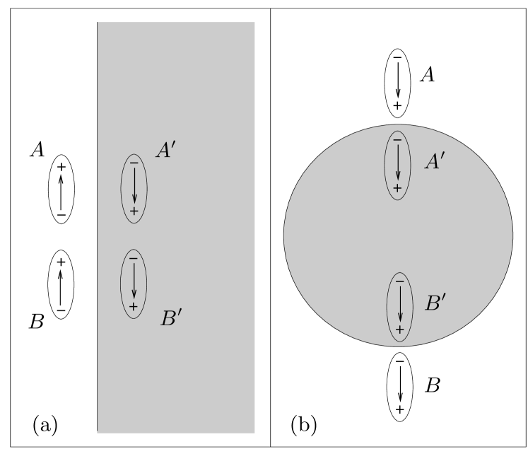
Figure 5: Two electric dipoles near a purely electrically polarizable sphere are shown in a triangulare configuration where the dipole-dipole angular separation (a) is small enough to replace the sphere, approximately, by a halfspace and (b) is equal to $\pi$.

The orientations of the dipoles $A$ and $B$ are random and independent of each other, so that strictly speaking the signs of all dipole–dipole interactions has to be obtained by averaging over all possible orientations. The effect of such averaging on the sign of the interactions can be reproduced by restricting the attention to the maximally attractive case of both dipoles pointing in the same direction parallel to their connecting line, with the dipole–dipole interaction $\hat{V}_{AB}$ being negative in this case. The image dipoles ${A}^{\prime}$ and ${B}^{\prime}$ are constructed by appropriate reflection of the dipoles $A$ and $B$. The resulting signs of the interactions $\hat{V}_{AB^{\prime}}$ and $\hat{V}_{BA^{\prime}}$ between dipoles and image dipoles are negative/positive if the respective dipole moments are parallel/antiparallel.

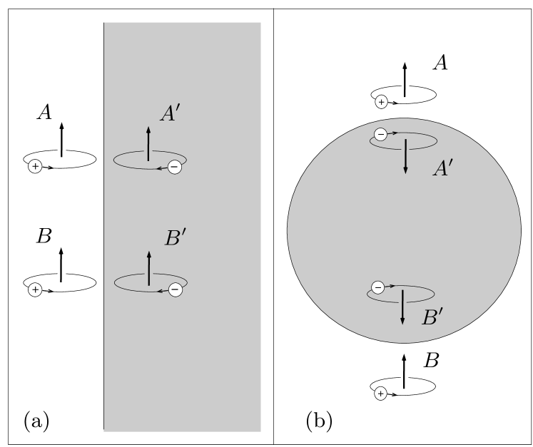
Figure 6: Two magnetic dipoles near a purely electrically polarizable sphere are shown in a triangulare configuration for a (a) very small angular separation (b) maximal angular separation.

Figure 5 shows two electric dipoles near a purely electrically polarizable sphere in the triangular configuration together with their images in the sphere. When the inter-dipole angular separation is very small, the curvature of the spherical surface can be disregarded and the sphere can be approximately replaced by a half space as in Fig. 5(a). It is seen that $U^{(1)}$, which is a product of one indirect and one direct interaction, is positive. Since the negative $U^{(2)}$ is a product of two indirect interactions, and the direct interaction is stronger than indirect one for small interatomic separations the sum $U^{(1)}+U^{(2)}$ is positive and hence the total potential $U_{AB}$ is weakened compared to that in free space. This confirms the numerical results for short distances presented in Fig. 3(a). The case of two dipoles located at the opposite ends of a sphere diameter is sketched in Fig. 5(b). It can be seen that $U^{(1)}$ is negative. As a consequence, $U_{AB}$ is enhanced in agreement with the curves in Fig. 3(a).

The case of two electric dipoles near a purely magnetically polarizable sphere can be treated by considering two magnetic dipoles near a purely electrically polarizable sphere, since the two situations are equivalent due to the duality between electric and magnetic fields. Again we consider the triangular configuration. In the limit of small separation angles, the surface can be regarded as flat. The sketch of the dipoles and their images in Fig. 6(a) indicates a negativeness of $U^{(1)}$ leading to an enhancement of the overall interaction potential [cf. Fig. 3(b) inset, solid curve]. When the separation angle is large (atoms located on opposite sides of the sphere), it can be inferred from Fig. 6(b) that $U^{(1)}$ is positive, resulting in a reduction of the interaction potential, in agreement with the numerical results shown in Fig. 3(b).

We turn now to the linear configuration. For dipoles situated near a purely electrically polarizable sphere [Fig. 7(a)], $U^{(1)}$ is negative resulting in an enhancement of the total interaction potential for all distance regimes as visible in Fig. 4(a). For a purely magnetically polarizable sphere, we again invoke the duality principle to replace it by a purely electrically polarizable one, and the electric dipoles by magnetic ones as shown in Fig. 7(b). It can be inferred from the sketch that $U^{(1)}$ is positive for all distances. In order to be conclusive about the body-induced effects, one hence has to compare the magnitudes of the competing $U^{(1)}$ and $U^{(2)}$. For small atom–atom separations, the direct interaction dominates, so $U^{(1)}$ is stronger than $U^{(2)}$ and the potential is reduced as shown in Fig. 4(b), inset. As the interatomic separation increases, the indirect interaction gains in relevance and hence $U^{(2)}$ may become dominant leading to an enhancement of the total vdW potential, in agreement with the curves presented in Fig. 4(b).

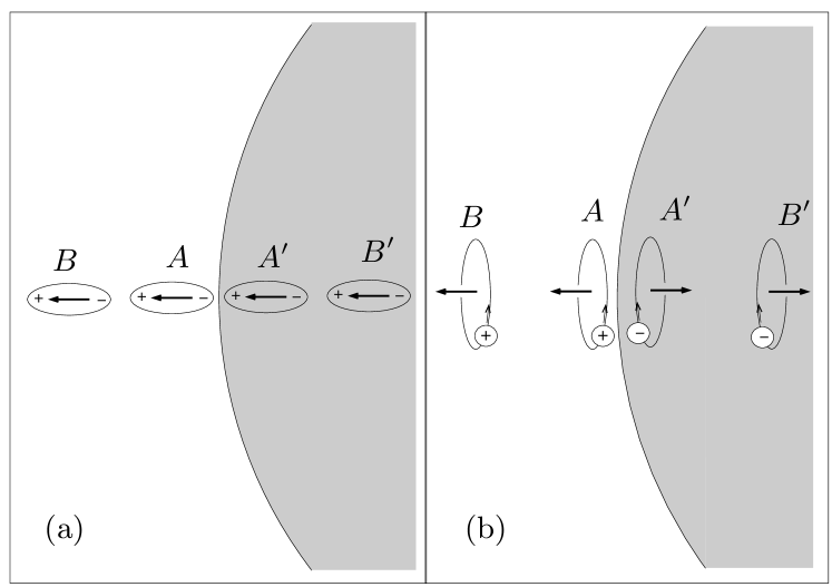
Figure 7: Two dipoles near a sphere are shown in a linear configuration. Figure 7(a) is showing two electric dipoles while in Fig. 7(b) two magnetic dipoles are shown.

V Summary

We have studied the mutual vdW interaction between two atoms near a dispersing and absorbing magneto-electric sphere and presented both analytical and numerical results. When the radius of the sphere becomes sufficiently large, then the interaction potential tends to the one found for two atoms near a magneto-electric half space. In the opposite case of a very small sphere, the sphere can be regarded as being a third atom with respective electric and magnetic polarizabilities. In particular for electrically polarizable atoms, the three-atom interaction potential is recovered.

The numerical calculations performed for medium-sized spheres show that—compared to the case of the atoms being in free space—the interatomic vdW interaction can be enhanced as well as reduced, depending on the electromagnetical properties of the sphere, the positions of the atoms relative to the sphere, and the positions of the atoms relative to each other. In general, the electric properties of the sphere have a more pronounced influence on the potential than the magnetic properties. We have shown that the behavior of the interatomic potential can be qualitytively understood in the basis of an image-charge model.

The results also indicate an essential difference between finite- and infinite-sized systems, which particularly becomes apparent in the linear configuration with a purely electrically polarizable sphere. Depending on the distance between the surface and the neighbouring atom, the (normalized) potential here approach different values, while in the case of a half-space they converge to a single value.

Appendix A Derivation of Eqs. (24)–(26)

To perform the summations over $m$ and $p$ in Eq. (17), we begin with the case $p$ $\!=$ $\!-1$ and evaluate the first term in the square brackets. Using Eqs. (18) and (22), we may write

$$\sum_{m=0}^{n}C_{nm}\mathbf{M}_{nm,-1}(\mathbf{r}_{A},k)\mathbf{M}_{nm,-1}(\mathbf{r}_{B},k)=\frac{Q^{(0)}_{n}\mathbf{e}_{\theta_{A}}\mathbf{e}_{\theta_{B}}}{\sin\theta_{A}\sin\theta_{B}}\\ \times\sum_{m=0}^{n}C_{nm}m^{2}\cos(m\pi)P_{n}^{m}(\cos\theta_{A})P_{n}^{m}(\cos\theta_{B}),$$ (63)

where

$$C_{nm}\equiv\frac{(n-m)!}{(n+m)!}(2-\delta_{0m}).$$ (64)

Differentiating the addition theorem for spherical harmonics

$$\sum_{m=0}^{n}C_{nm}P_{n}^{m}(\cos\theta)P_{n}^{m}(\cos\theta^{\prime})\cos(m\phi)=P_{n}(\psi),$$ (65)

where

$$\psi=\cos\theta\cos\theta^{\prime}+\sin\theta\sin\theta^{\prime}\cos\phi,$$ (66)

twice with respect to $\phi$, we obtain

$$\sum_{m=0}^{n}C_{nm}m^{2}\cos(m\phi)P_{n}^{m}(\cos\theta)P_{n}^{m}(\cos\theta^{\prime})\\ =-\frac{{\mathrm{d}}^{2}P_{n}(\psi)}{{\mathrm{d}}\psi^{2}}\biggl{(}\frac{{\mathrm{d}}\psi}{{\mathrm{d}}\phi}\biggr{)}^{2}-\frac{{\mathrm{d}}P_{n}(\psi)}{{\mathrm{d}}\psi}\frac{{\mathrm{d}}^{2}\psi}{{\mathrm{d}}\phi^{2}}.$$ (67)

Using Eq. (67) together with Eq. (66) in Eq. (63), we find that

$$\sum_{m=0}^{n}C_{nm}\mathbf{M}_{nm,-1}(\mathbf{r}_{A},k)\mathbf{M}_{nm,-1}(\mathbf{r}_{B},k)\\ =-Q^{(0)}_{n}\,\frac{\mathrm{d}P_{n}(\gamma)}{\mathrm{d}\gamma}\,\mathbf{e}_{\theta_{A}}\mathbf{e}_{\theta_{B}}$$ (68)

(recall that $\gamma$ $\!=$ $\!\cos\Theta$, $\Theta$ $\!=$ $\!\theta_{A}$ $\!+$ $\!\theta_{B}$). The summation over $m$ in the other terms in Eq. (17) can be performed in a similar way to obtain

$$\sum_{m=0}^{n}C_{nm}\mathbf{M}_{nm,+1}(\mathbf{r}_{A},k)\mathbf{M}_{nm,+1}(\mathbf{r}_{B},k)\\ =Q^{(0)}_{n}F_{n}(\gamma)\mathbf{e}_{\phi_{A}}\mathbf{e}_{\phi_{B}},$$ (69)

$$\sum_{m=0}^{n}C_{nm}\mathbf{N}_{nm,-1}(\mathbf{r}_{A},k)\mathbf{N}_{nm,-1}(\mathbf{r}_{B},k)\\ =-\frac{c^{2}}{\omega^{2}r_{A}r_{B}}Q^{(3)}_{n}P^{\prime}_{n}(\gamma)\mathbf{e}_{\phi_{A}}\mathbf{e}_{\phi_{B}},$$ (70)

$$\sum_{m=0}^{n}C_{nm}\mathbf{N}_{nm,+1}(\mathbf{r}_{A},k)\mathbf{N}_{nm,+1}(\mathbf{r}_{B},k)\\ =\frac{c^{2}}{\omega^{2}r_{A}r_{B}}\Bigl{\{}[n(n+1)]^{2}Q_{n}^{(1)}P_{n}(\gamma)\mathbf{e}_{r_{A}}\mathbf{e}_{r_{B}}\\ +n(n+1)\sin\Theta P^{\prime}_{n}(\gamma)\left[Q_{n}^{(2)}\mathbf{e}_{r_{A}}\mathbf{e}_{\theta_{B}}+Q_{n}^{(3)}\mathbf{e}_{\theta_{A}}\mathbf{e}_{r_{B}}\right]\\ -Q_{n}^{(4)}F_{n}(\gamma)\mathbf{e}_{\theta_{A}}\mathbf{e}_{\theta_{B}}\Bigr{\}}.$$ (71)

Inserting Eqs. (68)–(71) in Eq. (17), we arrive at Eqs. (24)–(26).

Appendix B The potential contributions $\bm{U_{ij}^{(1)}}$, Eq.(37), and $\bm{U_{ij}^{(1)}}$, Eq.(38)

We substitute Eqs. (32)–(35) together with Eqs. (24)–(26) into Eqs. (37) and (38) and obtain the following expressions for the nonzero $U^{(1)}_{ij}$ and $U^{(2)}_{ij}$:

$$U^{(1)}_{rr}(\mathbf{r}_{A},\mathbf{r}_{B})=-\frac{\hbar\mu_{0}^{2}c^{3}}{16\pi^{3}l^{5}r_{A}r_{B}}\sum_{n=1}^{\infty}n(n+1)(2n+1)P_{n}(\gamma)\\ \times\int_{0}^{\infty}{\mathrm{d}}u\,u\,e^{-lu/c}\alpha_{A}(iu)\alpha_{B}(iu)B_{n}^{N}(iu)Q_{n}^{(1)}\\ \times\left[l^{2}f(\xi)\cos\Theta-g(\xi)l_{A}l_{B}\right],$$ (72)

$$U^{(1)}_{\genfrac{}{}{0.0pt}{}{r\theta}{\theta r}}(\mathbf{r}_{A},\mathbf{r}_{B})=-\frac{\hbar\mu_{0}^{2}c^{3}\sin^{2}\Theta}{16\pi^{3}l^{5}r_{A}r_{B}}\sum_{n=1}^{\infty}(2n+1)P_{n}^{\prime}(\gamma)\\ \times\int_{0}^{\infty}{\mathrm{d}}u\,u\,e^{-lu/c}\alpha_{A}(iu)\alpha_{B}(iu)B_{n}^{N}(iu)\genfrac{}{}{0.0pt}{}{Q_{n}^{(2)}}{Q_{n}^{(3)}}\\ \times\left[l^{2}f(\xi)\pm g(\xi)r_{A(B)}l_{A(B)}\right],$$ (73)

$$U^{(1)}_{\theta\theta}(\mathbf{r}_{A},\mathbf{r}_{B})=\frac{\hbar\mu_{0}^{2}c}{16\pi^{3}l^{5}}\sum_{n=1}^{\infty}\frac{(2n+1)}{n(n+1)}\int_{0}^{\infty}{\mathrm{d}}u\,u^{3}\,e^{-lu/c}\\ \times\!\alpha_{A}(iu)\alpha_{B}(iu)\biggl{[}B_{n}^{M}(iu)Q_{n}^{(1)}P^{\prime}_{n}(\gamma)-\frac{c^{2}B_{n}^{N}(iu)}{u^{2}r_{A}r_{B}}\\ \times Q_{n}^{(4)}F_{n}(\gamma)\biggr{]}\!\left[l^{2}f(\xi)\cos\Theta-g(\xi)r_{A}r_{B}\sin^{2}\Theta\right],$$ (74)

$$U^{(1)}_{\phi\phi}(\mathbf{r}_{A},\mathbf{r}_{B})=\frac{\hbar\mu_{0}^{2}c}{16\pi^{3}l^{3}}\sum_{n=1}^{\infty}\frac{(2n+1)}{n(n+1)}\int_{0}^{\infty}{\mathrm{d}}u\,u^{3}\,e^{-lu/c}\\ \times\!\alpha_{A}(iu)\alpha_{B}(iu)\biggl{[}B_{n}^{M}(iu)Q_{n}^{(1)}F_{n}(\gamma)\\ -\frac{c^{2}B_{n}^{N}(iu)}{u^{2}r_{A}r_{B}}\,Q_{n}^{(4)}P_{n}^{\prime}(\gamma)\biggr{]}f(\xi),$$ (75)

$$U^{(2)}_{rr}(\mathbf{r}_{A},\mathbf{r}_{B})\!=\!\frac{-\hbar\mu_{0}^{2}c^{2}}{32\pi^{3}r_{A}^{2}r_{B}^{2}}\!\sum_{m,n=1}^{\infty}m(m\!+\!1)(2m\!+\!1)\\ \times n(n\!+\!1)(2n\!+\!1)P_{m}(\gamma)P_{n}(\gamma)\int_{0}^{\infty}{\mathrm{d}}u\,u^{2}\\ \times\alpha_{A}(iu)\alpha_{B}(iu)B_{m}^{N}(iu)B_{n}^{N}(iu)Q_{m}^{(1)}Q_{n}^{(1)},$$ (76)

$$U^{(2)}_{\genfrac{}{}{0.0pt}{}{r\theta}{\theta r}}(\mathbf{r}_{A},\mathbf{r}_{B})\!=\!\frac{-\hbar\mu_{0}^{2}c^{2}\sin^{2}\Theta}{32\pi^{3}r_{A}^{2}r_{B}^{2}}\!\sum_{m,n=1}^{\infty}(2m\!+\!1)(2n\!+\!1)\\ \times\!P_{m}^{\prime}(\gamma)P_{n}^{\prime}(\gamma)\int_{0}^{\infty}{\mathrm{d}}u\,u^{2}\alpha_{A}(iu)\alpha_{B}(iu)\\ \times B_{m}^{N}(iu)B_{n}^{N}(iu)\genfrac{}{}{0.0pt}{}{Q_{m}^{(2)}Q_{n}^{(2)}}{Q_{m}^{(3)}Q_{n}^{(3)}},$$ (77)

$$U^{(2)}_{\genfrac{}{}{0.0pt}{}{\theta\theta}{\phi\phi}}(\mathbf{r}_{A},\mathbf{r}_{B})=\frac{-\hbar\mu_{0}^{2}}{32\pi^{3}c^{2}}\sum_{m,n=1}^{\infty}\frac{(2n\!+\!1)}{n(n\!+\!1)}\frac{(2m\!+\!1)}{m(m\!+\!1)}\\ \times\int_{0}^{\infty}{\mathrm{d}}u\,u^{6}\alpha_{A}(iu)\alpha_{B}(iu)\biggl{[}B_{m}^{M}Q_{m}^{(1)}\genfrac{}{}{0.0pt}{}{P^{\prime}_{m}(\gamma)}{F_{m}(\gamma)}\\ -\frac{c^{2}B_{m}^{N}}{u^{2}r_{A}r_{B}}Q_{m}^{(4)}\genfrac{}{}{0.0pt}{}{F_{m}(\gamma)}{P_{m}^{\prime}(\gamma)}\biggr{]}\biggl{[}B_{n}^{M}Q_{n}^{(1)}\genfrac{}{}{0.0pt}{}{P^{\prime}_{n}(\gamma)}{F_{n}(\gamma)}\\ -\frac{c^{2}B_{n}^{N}}{u^{2}r_{A}r_{B}}Q_{n}^{(4)}\genfrac{}{}{0.0pt}{}{F_{n}(\gamma)}{P_{n}^{\prime}(\gamma)}\biggr{]}.$$ (78)

Appendix C The limiting cases of a large and a small sphere

When in the case of a large sphere the conditions (39) and (40) are satisfied, then the leading contributions to the sums in Eqs. (24)–(26) come from terms with $n$ $\!\gg$ $\!1$ (also see Ref. st1 ), for which the spherical Bessel and Hankel functions approximate to abr

$$j_{n}(z)=\frac{z^{n}}{(2n+1)!!}\left[1-\frac{z^{2}}{4n+6}+\frac{z^{4}}{(16n+24)(2n+5)}\right]$$ (79)

and

$$h_{n}^{(1)}(z)=-i\frac{(2n-1)!!}{z^{n+1}}\!\left[1\!+\!\frac{z^{2}}{4n-2}\!+\!\frac{z^{4}}{(16n-8)(2n-3)}\right]\!,$$ (80)

respectively. Hence, Eqs. (20) and (21) approximate to

$$B_{n}^{M}(iu)=\frac{i(iRu/c)^{2n+1}}{16n[(2n+1)!!]^{2}[\mu(iu)+1]}\left(a_{2}n^{2}\!+\!a_{1}n\!+\!a_{0}\right)$$ (81)

and

$$B_{n}^{N}(iu)=\frac{i(iRu/c)^{2n+1}}{16n[(2n+1)!!]^{2}[\varepsilon(iu)+1]}\left(b_{2}n^{2}\!+\!b_{1}n\!+\!b_{0}\right)\!,$$ (82)

respectively, where

$$a_{0}=\left\{488+[1+\varepsilon(iu)\mu(iu)]^{2}R^{4}u^{4}/c^{4}\right\}[\mu(iu)-1]\\ -8\left\{7\mu(iu)[\varepsilon(iu)\!-\!1]\!-\!5\varepsilon(iu)\mu(iu)^{2}\!+\!5\right\}R^{2}u^{2}/c^{2},$$ (83)

$$a_{1} =8\left\{26+[1+\varepsilon(iu)\mu(iu)]R^{2}u^{2}/c^{2}\right\}[\mu(iu)-1]$$

$$\equiv 8\eta(iu)[\mu(iu)-1],$$ (84)

$$a_{2}=32[\mu(iu)-1],$$ (85)

and $b_{0}$, $b_{1}$, and $b_{2}$ can be found from $a_{0}$, $a_{1}$, and $a_{2}$, respectively, by interchanging $\mu$ and $\varepsilon$. Equations (27)–(30) then approximate to

$$Q_{n}^{(1)}=-\left(\frac{ic}{u}\right)^{2n+2}\frac{[(2n-1)!!]^{2}}{(r_{A}r_{B})^{n+1}},$$ (86)

$$Q_{n}^{(2)}=Q_{n}^{(3)}=-Q_{n}^{(4)}/n=-nQ_{n}^{(1)}.$$ (87)

In order to illustrate the application of the approximation scheme to the Green tensor elements (24)–(26), let us consider the element $G_{rr}^{(1)}(\mathbf{r}_{A},\mathbf{r}_{B},iu)$. Inserting Eqs. (82) and (86) in Eq. (24), we find

$$G_{rr}^{(1)}(\mathbf{r}_{A},\mathbf{r_{B}},iu)=\frac{-c^{2}t}{128\pi u^{2}R^{3}[\varepsilon(iu)+1]}\sum_{k=0}^{2}a_{k}s_{k},$$ (88)

where

$$s_{k}=\sum_{n=1}^{\infty}n^{k}t^{n+1}P_{n}(\gamma)$$ (89)

and $t$ $\!=$ $\!R^{2}/(r_{A}r_{B})$. Differentiating the identity

$$\sum_{n=1}^{\infty}t^{n}P_{n}(\gamma)=\frac{1}{\sqrt{1-2t\gamma+t^{2}}}-1$$ (90)

abr with respect to $t$, we can perform the summation in Eq. (88) to obtain

$$s_{0}=\frac{t}{\sqrt{1-2t\gamma+t^{2}}}-t,$$ (91)

$$s_{1}=\frac{t^{2}\gamma-t^{3}}{\left[1-2t\gamma+t^{2}\right]^{3/2}}$$ (92)

$$s_{2}=\frac{3\gamma^{2}-4\gamma t+2t^{2}-1}{\left[1-2t\gamma+t^{2}\right]^{5/2}}$$ (93)

Recalling the conditions (39) and (40), we can further simplify the result. Up to second order in the small parameters $\delta_{A^{\prime}}/R$, we have

$$t^{k}=1-k\frac{\delta_{A}+\delta_{B}}{R}+\frac{k(k+1)}{2}\frac{\delta_{A}^{2}+\delta_{B}^{2}}{R^{2}}+k^{2}\frac{\delta_{A}\delta_{B}}{R^{2}},$$ (94)

implying that

$$1-2t\gamma+t^{2}\simeq\Theta^{2}+\frac{(\delta_{A}+\delta_{B})^{2}}{R^{2}}=\frac{l_{+}^{2}}{R^{2}}.$$ (95)

Using Eqs. (91)–(95) in Eq. (88), we find that within this order,

$$G_{rr}^{(1)}(\mathbf{r}_{A},\mathbf{r_{B}},iu)=\frac{c^{2}}{128\pi u^{2}l_{+}^{5}[\varepsilon(iu)+1]}\\ \times\bigg{\{}32(X^{2}-2\delta_{+}^{2})[\varepsilon(iu)-1]-8\frac{\delta_{+}l_{+}^{2}}{R}\eta(iu)[\varepsilon(iu)-1]\\ -\bigg{[}\bigg{(}488+[1+\varepsilon(iu)\mu(iu)]^{2}\frac{R^{4}u^{4}}{c^{4}}\bigg{)}[\varepsilon(iu)-1]\\ -8\Big{[}7\varepsilon(iu)[\mu(iu)\!-\!1]\!-\!5\varepsilon^{2}(iu)\mu(iu)\!+\!5\Big{]}\frac{R^{2}u^{2}}{c^{2}}\bigg{]}\frac{l_{+}^{4}}{R^{2}}\bigg{\}}.$$ (96)

Recalling that $X$, $l_{+}$, $\delta_{+}$ $\!\ll$ $\!R$, it can be seen that unless $|\varepsilon(iu)$ $\!-$ $\!1|$ $\!\ll$ $\!1$, the third term in the curly bracket in Eq. (96) can be approximately ignored. Hence,

$$G_{rr}^{(1)}(\mathbf{r}_{A},\mathbf{r_{B}},iu)=\frac{c^{2}}{4\pi u^{2}l_{+}^{5}}\frac{\varepsilon(iu)-1}{\varepsilon(iu)+1}\\ \times\left\{(X^{2}-2\delta_{+}^{2})-\frac{\delta_{+}l_{+}^{2}}{16R}\left[26+\varepsilon(iu)\mu(iu)R^{2}u^{2}/c^{2}\right]\right\}\!.$$ (97)

In the case of a purely magnetically polarizable sphere [$\varepsilon(iu)$ $\!=$ $\!1$], the leading contribution to $G_{rr}^{(1)}$ comes from the third term in the curly brackets in Eq. (96):

$$G_{rr}^{(1)}(\mathbf{r}_{A},\mathbf{r_{B}},iu)=\frac{\mu(iu)-1}{16\pi l_{+}}.$$ (98)

The other Green tensor elements can be evaluated in a quite similar way. Substituting the resulting expressions into Eqs. (37) and (38), and summing them in accordance with Eq. (36), we eventually arrive at Eqs. (41) and (43).

In the limiting case of a small sphere where the condition (44) holds, the leading contributions to the frequency integrals in Eqs. (72)–(78) come from the region where $u$ $\!\ll$ $\!c/R$, or equivalently $|z_{0}|$, $|z_{1}|$ $\!\ll$ $\!1$ (also see Ref. st1 ). In this region we may approximate the spherical Bessel and Hankel functions appearing in Eqs. (20) and (21) by their next-to-leading order expansions in $z$ abr , i.e.,

$$j_{n}(z)=\frac{z^{n}}{(2n+1)!!}\left[1-\frac{z^{2}}{4n+6}\right]$$ (99)

and

$$h_{n}^{(1)}(z)=-i\frac{(2n-1)!!}{z^{n+1}}\left[1-\frac{z^{2}}{2-4n}\right],$$ (100)

so that Eqs. (20) and (21), respectively, approximate to

$$B_{n}^{M}(iu)=i\frac{2n+1}{[(2n+1)!!]^{2}[\mu(iu)n+n+1]}\\ \times\left\{[\mu(iu)-1](n+1)\left(\frac{iRu}{c}\right)^{\!2n+1}+O\!\left(\frac{iRu}{c}\right)^{\!2n+3}\right\}$$ (101)

and

$$B_{n}^{N}(iu)=i\frac{2n+1}{[(2n+1)!!]^{2}[\varepsilon(iu)n+n+1]}\\ \times\left\{[\varepsilon(iu)-1](n+1)\left(\frac{iRu}{c}\right)^{\!2n+1}+O\!\left(\frac{iRu}{c}\right)^{\!2n+3}\right\},$$ (102)

revealing that in Eq. (36) the $U_{ij}^{(2)}$ terms are small in comparison to the $U_{ij}^{(1)}$ terms and can be neglected, so that, in leading order of $Ru/c$,

$$U^{(b)}=\sum_{i,j=r,\theta,\phi}U^{(1)}_{ij}(\mathbf{r}_{A},\mathbf{r}_{B}).$$ (103)

Further, it can be seen that in the sums in Eqs. (24)–(26) the terms with $n$ $\!=$ $\!1$ are the leading ones, for which

$$Q_{1}^{(1)}=-\frac{(1+a)(1+b)}{a^{2}b^{2}}\,e^{-a-b},$$ (104)

$$Q_{1}^{(2)}=\frac{(1+a)f(b)}{a^{2}b^{2}}\,e^{-a-b},$$ (105)

$$Q_{1}^{(3)}=\frac{f(a)(1+b)}{a^{2}b^{2}}\,e^{-a-b},$$ (106)

$$Q_{1}^{(4)}=-\frac{f(a)f(b)}{a^{2}b^{2}}\,e^{-a-b},$$ (107)

$$F_{1}(\gamma)=P_{1}(\gamma)=\gamma,$$ (108)

$$B_{1}^{M}(iu)=\frac{2}{3}\frac{\mu(iu)-1}{\mu(iu)+2}\left(\frac{Ru}{c}\right)^{3},$$ (109)

$$B_{1}^{N}(iu)=\frac{2}{3}\frac{\varepsilon(iu)-1}{\varepsilon(iu)+2}\left(\frac{Ru}{c}\right)^{3}.$$ (110)

Substituting Eqs. (72)–(75) together with Eqs. (104)–(110) in Eq. (103), we arrive at Eq. (45).

References

- (1) S. Y. Buhmann and D.-G. Welsch, Prog. Quant. Electron. 31, 51 (2007).
- (2) F. London, Z. Phys. 63, 245 (1930); Z. Phys. Chem. Abt. B 11, 222 (1930).
- (3) H. B. G. Casimir and D. Polder, Phys. Rev. 73, 360 (1948).
- (4) T. Emig, N. Graham, R. L. Jaffe, and M. Kardar, Phys. Rev. Lett. 99, 170403 (2007).
- (5) B. M. Axilrod and E. Teller, J. Chem. Phys. 11, 299 (1943); B. M. Axilrod, J. Chem. Phys. 19, 719 (1951).
- (6) M. R. Aub and S. Zienau, Proc. R. Soc. London, Ser. A 257, 464 (1960).
- (7) E. A. Power and T. Thirunamachandran, Proc. R. Soc. London Ser. A 401, 267 (1985).
- (8) E. A. Power and T. Thirunamachandran, Phys. Rev. A 50, 3929 (1994).
- (9) A. D. McLachlan, Mol. Phys. 7, 381 (1964).
- (10) J. Mahanty and B. W. Ninham, J. Phys. A 6, 1140 (1973); J. Mahanty and B. W. Ninham, Dispersion Forces (Academic Press, London, 1976).
- (11) H. Safari, S. Y. Buhmann, D.-G. Welsch, and Ho Trung Dung, Phys. Rev. A 74, 042101 (2006);
- (12) S. Y. Buhmann, H. Safari, and D.-G. Welsch, Open Sys. & Information Dyn. 13, 427 (2006).
- (13) S. Spagnolo, D. A. R. Dalvit, and P. W. Milonni, Phys. Rev. A 75, 052117 (2007).
- (14) J. Mahanty, N. H. March, and B. V. Paranjape, Appl. Surf. Sci. 33/34, 309 (1988).
- (15) S. Spagnolo, R. Passante, and L. Rizzuto, Phys. Rev. A 73, 062117 (2006).
- (16) O. Sinanoǧlu and K. S. Pitzer, J. Chem. Phys. 32, 1279 (1960).
- (17) A. Sambale, S. Y. Buhmann, D.-G. Welsch, and M. S. Tomaš, Phys. Rev. A 75, 042109 (2007).
- (18) M. S. Tomaš, Phys. Rev. A 75, 012109 (2007).
- (19) C. I. Sukenik, M. G. Boshier, D. Cho, V. Sandoghdar, and E. A. Hinds, Phys. Rev. Lett. 70, 560 (1993).
- (20) A. Landragin, J.-Y. Courtois, G. Labeyrie, N. Vansteenkiste, C. I. Westbrook, and A. Aspect, Phys. Rev. Lett. 77, 1464 (1996).
- (21) A. K. Mohapatra and C. S. Unnikrishnan, Europhys. Lett. 73, 839 (2006).
- (22) R. E. Grisenti, W. Schöllkopf, and J. P. Toennies, G. C. Hergerfeldt, and T. Kohler, Phys. rev. Lett. 83, 1755 (1999).
- (23) V. Druzhinina and M. DeKieviet, Phys. Rev. Lett. 91, 193202 (2003).
- (24) T. A. Pasquini, Y. Shin, C. Sanner, M. Saba, A. Schirotzek, D. E. Pritchard, and W. Ketterle, Phys. Rev. Lett. 93, 223201 (2004).
- (25) T. A. Pasquini, M. Saba, G.-B. Jo, Y. Shin, W. Ketterle, and D. E. Pritchard, Phys. Rev. Lett. 97, 093201 (2006).
- (26) J. M. Obrecht, R. J. Wild, M. Antezza, L. P. Pitaevskii, S. Stringari, and E. A. Cornell, Phys. Rev. Lett. 98, 063201 (2007).
- (27) C. H. Chen, P. E. Siska, and Y. T. Lee, J. Chem. Phys. 59, 601 (1973).
- (28) B. Brunetti, F. Pirani, Vecchiocattivi, and E. Luzzatti, Chem. Phys. Lett. 55, 565 (1978)
- (29) B. Brunetti, G. Luiti, E. Luzzatti, F. Pirani, and G. G. Volpi, J. Chem. Phys. 79, 273 (1983)
- (30) D. W. Martin, R. W. Gregor, R. M. Jordan, and P. E. Siska, J. Chem. Phys. 69, 2833 (1987).
- (31) S. Y. Buhmann, Ho Trung Dung, and D.-G. Welsch, J. Opt. B: Quantum Semiclass. Opt. 6, S127 (2004).
- (32) L. Knöll and D.-G. Welsch, Prog. Quant. Electron. 16, 135 (1992).
- (33) Le-Wei Li, Pang-Shyan Kooi, Mook-Seng Leong, and Yeo, IEEE Trans. Microwave Theory Tech. 42, 2302 (1994).
- (34) R. Passante, F. Persico, and L. Rizzuto, J. Phys. B: At. Mol. Opt. Phys. 39, 685 (2006).
- (35) M. Abramowitz and I. A. Stegun, Pocketbook of Mathematical Functions (Verlag Harri Deutsch, Frankfurt, 1984).