Optimization code with weighting function for the reconstruction of coronal magnetic fields.
Bibliographic Code: 2004SoPh..219…87W)
Abstract
We developed a code for the reconstruction of nonlinear force-free and not force-free coronal magnetic fields. The 3D magnetic field is computed numerically with the help of an optimization principle. The force-free and non force-free codes are compiled in one program. The force-free approach needs photospheric vectormagnetograms as input. The non force-free code additional requires the line-of-sight integrated coronal density distribution in combination with a tomographic inversion code. Previously the optimization approach has been used to compute magnetic fields using all six boundaries of a computational box. Here we extend this method and show how the coronal magnetic field can be reconstructed only from the bottom boundary, where the boundary conditions are measured with vector magnetographs. The program is planed for use within the Stereo mission.
keywords:
coronal magnetic fields, Stereo, MHD:
JEL codesAppl. Opt.
Kluwer Prepress Department
P.O. Box 990
3300 AZ Dordrecht
The Netherlands
KAPKluwer Academic Publishers; \abbrevcompuscriptElectronically submitted article
KAPKluwer Academic Publishers; \nomencompuscriptElectronically submitted article
D24, L60, 047
1 Introduction
The solar magnetic field is an important quantity which couples the solar interior with the photosphere and atmosphere. Knowledge regarding the coronal magnetic field plays a key role for eruptive phenomena, e.g. coronal mass ejection, flares and eruptive prominences. Unfortunately a direct measurement of the coronal magnetic field is extremely difficult. In principle one can use the polarization of emissions from magnetic sensitive coronal line transitions to draw conclusions about the coronal magnetic field. These lines, however, are very faint so that in the past they have only occasionally been observed (e.g., [House (1977), Arnaud and Newkirk (1987), Judge (1998)]). In a recent study [Judge et al. (2001)] conclude that several forbidden lines (e.g. in Fe XIII, He I, Mg VIII and Si IX) may be used to determine the coronal magnetic field. They further concluded that space born missions are not needed for such kind of coronal magnetometers but a high, dry mountain site. In their study they propose a focal plane instrument devoted to the region. These authors also point out that besides the observational part, a further major problem is the interpretation of the data. The line-of-sight integration inherent in these observations make the data analysis a badly posed inversion problem. Presently, algorithms based on vector tomography are studied to find out to which extend the coronal magnetic field can be reconstructed from these observations (Maxim Kramar and Bernd Inhester, private communication).
Despite these promising new developments regarding the principle possibility of coronal B-field measurements we have to face the fact that currently and probably also in near future high quality direct measurements of the coronal magnetic field are not available. As an alternative to the above measurements, a number of authors have modelled the coronal magnetic field by extrapolation from more sound photospheric magnetic field observations.
It is generally assumed that the magnetic pressure in the corona is much higher than the plasma pressure (small plasma ) and that therefore the magnetic field is nearly force-free (for a critical view of this assumption see [Gary (2001)]). The extrapolation methods based on this assumption include potential field extrapolation [Schmidt (1964), Semel (1967)], linear force-free field extrapolation [Chiu and Hilton (1977), Seehafer (1978), Seehafer (1982), Semel (1988)] and nonlinear force-free field extrapolation [Amari et al. (1997)]. Methods for the extrapolation non force-free fields and have been developed by [Petrie and Neukirch (2000), Wiegelmann and Inhester (2003)]. Potential fields can be determined directly from line-of-sight magnetogram data (e.g. MDI on SOHO). Linear force-free fields can as well be calculated from line-of-sight magnetograms, but contain a free parameter which has to be computed from additional data, e.g. with fitting procedures which try to match the field model with observed coronal plasma loops using data from e.g. EIT [Wiegelmann and Neukirch (2002)] or Yohkoh [Carcedo et al. (2003)]. Unfortunately potential fields and linear force-free fields do not contain free energy and are very probably a poor approximation for an active region prior to an eruption. By free energy we understand energy which can be released during an eruption. A linear force free field has more energy than a potential field. This energy can, however, not be released during an eruption related to ideal or resistive MHD-instabilities because a linear force free field cannot rapidly relax to a potential field. The reason is that the magnetic helicity is strictly conserved for ideal MHD and approximately conserved for resistive processes. (The magnetic helicity is dissipated slower than the magnetic energy, see [Berger (1984)]). A nonlinear force free field can, however, relax to a linear force free field with the same magnetic helicity. In this sense a nonlinear force free field has free energy available for an eruption. Consequently investigations regarding non-linear force-free fields are essential to understand eruptive phenomena.
The calculation of non linear force-free fields is complicated by the intrinsic nonlinearity of the underlying mathematical problem. From the observational point of view the non linear reconstruction is also more challenging because photospheric vector magnetograph data are required. Unfortunately the transversal component of the photospheric B-field is measured with significant lower accuracy as the line of sight component. An additional problem is that the transversal magnetic field is only known with respect to an ambiguity and a preprocessing of the raw data is necessary to resolve this ambiguity (One possibility is the minimum energy method by [Metcalf (1994)] used for vector magnetogram data from IVM in Hawaii.).
Several methods have been proposed to compute nonlinear force-free fields:
-
•
A conceptionally simple method is to reformulate the force-free equations (2-3) in such way that they can be used for an upward integration of the vector magnetogram into the corona [Wu et al. (1990), Amari et al. (1997)]. This direct extrapolation is an ill posed problem for the elliptic equations (2-3) and consequently the method is limited to low heights. In particular one finds that an erroneous exponential growth of the magnetic field with increasing height is a typical behaviour.
-
•
An alternative approach is to use a Grad-Rubin method ([Sakurai (1981), (3)]). This method uses a potential field as initial equilibrium and then progressively currents are introduced into the system and the fields are relaxed towards a force-free state. The method is especial useful for small deviations from a potential field with small values of and modest non linearities. The method requires an explicit calculation of the distribution on the photosphere. In principle the computation of is straight forward but this is inaccurate for observational data for the following reasons. First one needs the transversal component of the photospheric magnetic field which is measured with lower accuracy than the line of sight magnetic field. In a second step one has to take the horizontal derivatives (x,y)of these inaccurate values and finally one has to divide through the normal magnetic field which causes additional problems where is small. These errors cumulate in the photospheric distribution.
-
•
A third possibility is to use the method of MHD relaxation [Chodura and Schlüter (1981), Roumeliotis (1996)]. The idea is to start with a suitable magnetic field which is not in equilibrium and to relax it into a force-free state. For test configurations [Low and Lou (1989)] the MHD relaxation method converges to the exact solution, but with less accuracy than the optimization approach discussed below [Wiegelmann and Neukirch (2003)].
-
•
In the optimization approach [Wheatland et al. (2000)] a functional containing the force-free equations is minimized. The method directly uses the measured vector magnetograph data and an explicit computation of is not necessary. Another advantage of the method is that the quality of the reconstructed magnetic field (force-free and solenoidal condition) is controlled automatically within the iteration procedure. A difficulty of the method is that it requires boundary conditions on all boundaries of a computational box while for observational data only the bottom boundary data are known. Within this paper we are dealing with this problem and extend the optimization method accordingly.
While the low plasma in the lower corona can be described with the non linear force-free approach, it is necessary to include plasma pressure and solar gravitation to describe regions with a finite plasma , e.g. helmet streamers. [Wiegelmann and Inhester (2003)] extended the force-free optimization with the aim to include these forces and showed that the method converges for test configurations. The difficulties regarding the lateral and top boundaries are analog to the non-linear force-free case. The non force-free reconstruction requires additional data as input, e.g. the coronal plasma density distribution from an assumed model or computed with help of tomographic methods.
We outline the paper as follows. In section 2 we provide the basic equations of the modified optimization method and derive the iteration equations. In section 3 we specify useful forms of the weighting function in the boundary regions. Section 4 contains test runs regarding the non linear force-free case and section 5 consistency checks for non force-free configurations. We draw conclusions in section 6 and give an outlook for further research.
2 Basic equations
Force-free coronal magnetic fields have to obey the equations
| (1) | |||||
| (2) | |||||
| (3) |
The force-free approach is valid in the low corona where the plasma is small. For extended structures, e.g. helmet streamers the plasma increases and the force-free assumption is not valid anymore. Therefore it is necessary to consider the effect of plasma pressure and gravity here and solve the magneto hydro static equations (MHS).
| (4) | |||||
| (5) | |||||
| (6) |
where is the magnetic field, the electric current density, the plasma pressure, the plasma density, the vacuum permeability and the solar gravity potential. We define the functional
| (7) |
with
| (10) | |||||
| (11) |
is a weighting function. Useful forms of the weighting function will be discussed below.
For the force-free case the functional is given explicitly as
| (12) |
and it is obvious that (for ) the force-free equations (1-3) are fulfilled when L is equal zero. For the non force-free case L is given explicitly as
| (13) |
and when the functional reaches (for ) its minimum at then the MHS equations (4-6) are fulfilled.
The following discussion is equivalent for the force-free and non force-free case. Without weighting function the method has been developed by [Wheatland et al. (2000)] for the force-free case and by [Wiegelmann and Inhester (2003)] for the non force-free case. For the optimization method requires that the magnetic field is given on all (6 for a rectangular computational box) boundaries. This causes a serious limitation of the method because such data are only available for model configurations. For the reconstruction of the coronal magnetic field it is necessary to develop a method which reconstructs the magnetic field only from photospheric vector magnetograms. Vector magnetograms provide boundary conditions only for the bottom boundary of a computational box while the other five boundaries remain unknown. Without a weighting function all six boundaries of the computational box have equal rights and influence the solution in the box. It is therefore important to diminish the effect of the top and lateral boundaries on the magnetic field inside the computational box. This can be done either by including a variation of B not only in the interior but also on those boundaries where B is unknown. This approach, however, is numerically difficult because it involves two types of variations. We show that it is essentially equivalent to introducing finite size boundary regions on those boundaries where B is unknown with the weighting function different from unity.
The idea is do define an interior physical region where we want to calculate the magnetic field so that it fulfills the force-free or MHS equations. This region is in the center of the box (including the photosphere) with . The computational box additionally includes boundary layers towards the lateral and top boundary where decreases to at the computational boundary. Consequently the method weights deviations from the force-free state (or MHS-state) less severely close to the boundary. The use of a weighting function has been proposed for the force-free case by [Wheatland et al. (2000)] in the conclusions but no iteration equations or test simulations have been presented. Here we provide these iteration equations for the more generalized case. We carry out several tests to investigate the optimum shape of the weighting function and how the size of the boundary layer influences the quality of the reconstruction.
We minimize equation (7) with respect to an iteration parameter (see Appendix A for details) and obtain an iteration equation for the magnetic field
| (14) |
| (15) | |||||
| (16) |
| (17) | |||||
| (18) |
and is the inward unit vector on the surface . The surface integral in (14) vanishes if the magnetic field is described on the boundaries of a computational box. Inside the computational box we iterate the magnetic field with
| (19) |
which insures that is monotonically decreasing.
2.1 Algorithm
We compute the 3D-coronal magnetic field in a numerical box using the following steps.
-
•
As a start configuration we use the measured normal component of the magnetic field to calculate a potential magnetic field in the whole box with help of a Fourier representation [Seehafer (1978)].
-
•
For non force-free (finite ) configurations the plasma density distribution is described in the box. This step is unnecessary for force-free fields.
-
•
We use vector magnetograph data to describe the bottom boundary (photosphere) of the computational box. On the lateral and top boundaries the field is chosen from the potential field above.
-
•
We iterate for the magnetic field inside the computational box with (19) using a Landweber-iteration (see e.g. [Louis (1989)]). The continuous form of (19) guaranties a monotonically decreasing . This is as well ensured in the discretized form if the iteration step is sufficiently small. The code checks if after each time step. If the condition is not fulfilled, the iteration step is repeated with reduced by a factor of 2. After each successful iteration step we increase slowly by a factor of to allow the time step to become as large as possible with respect to the stability condition. The iteration stops if falls below a limiting value, e.g. of the initial iteration step 111We find that the time step keeps on decreasing recurrently when the solution has converged. We never found a further improvement of L after has once fallen below of the initial iteration step. in the current version of the code.
Let us remark that the main numerics of the optimization code is similar for the method with and without a weighting function. The main problem for the optimization method without weighting function is that it requires the vector magnetic field on all six boundaries of a computational box. As only the bottom boundary is measured one has to make assumptions regarding the lateral and top boundary, e.g. assume a potential field. In general this leads to inconsistent boundary conditions (See [Aly (1989)] regarding the compatibility of photospheric vector magnetograph data.) and consequently a bad quality of the reconstructed magnetic field. With help of the weighting function the five inconsistent boundaries are replaced by boundary layers and consequently we get more flexible boundaries around the physical domain which will adjust automatically during the iteration. The idea of introducing a boundary layer with is to reduce the dependence of the solution in the interior of the box from the unknown boundary conditions. Since we have no measurements on these boundaries any choice of the boundary conditions is a mere guess. The aim is only to allow the solution in the interior to evolve more independently from the boundary conditions chosen. So the advantage of the boundary layer is a higher degree of independence of the solution in the interior from the chosen boundary. The price we have to pay is a higher computing time, as the magnetic field has to be iterated within the whole computational box which includes the physical domain as well as the boundary layers.
3 Special forms of the weighting function .
We want to use the weighting function to deal with the unknown top and lateral boundaries. We define an inner physical domain with and boundary layers where decreases monotonically from 1 to 0 through the outer numerical boundary layer with the thickness . Consequently becomes one-dimensional in each boundary layer (e.g. at the top boundary layer) and we get . The surface integrals vanish on all boundaries because on the top and lateral boundaries and on the bottom boundary where the magnetic field is measured with vectormagnetographs. Consequently (14) reduces to
| (20) | |||||
| (21) | |||||
| (22) | |||||
It is interesting to investigate the limit of an infinitesimally thin boundary layer in (22). The thinner the boundary layer becomes the steeper is and for an infinitesimally thin boundary layer the gradient becomes infinity. The boundary layer is constructed in such way that independent from the sheet thickness we have which remains true also for . In the limit of the term remains constant through the sheet and the integration regarding can be carried out explicitly. Consequently only a surface integral remains as the last term in equation (22). The second integral in (22) vanishes for and we get
| (23) |
This exactly coincides with the non weighted case. Consequently equation (22) is a generalization of the usual optimization equation (23).

4 Tests for non linear force-free configurations.
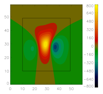
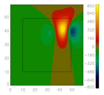
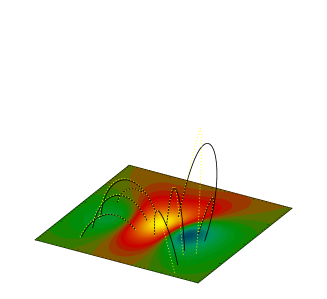

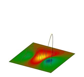
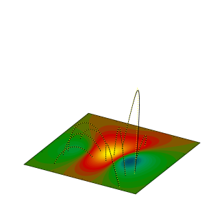
To test our code we use a semi-analytic model active region developed by [Low and Lou (1989)]. We use the Low and Lou solution with and as test. The normal photospheric magnetic field is normalized to a maximum of Gauss. Figure 2 shows the normal magnetic field on the photosphere for this configuration. The framed region contains the physical domain. We investigate two cases, in Force-Free I the physical domain is approximately flux-balanced and in Force-Free II not. We are interested in reconstructing an inner region (physical domain) of points and diagnose and averaged over the physical domain here. We also diagnose in the whole computational box.
At the lateral and top boundary we introduce an additional boundary layer of points and decreases from to in this layer. We investigate different profiles regarding the weighting function, e.g. linear, quadratic, cos and tanh (see figure 1). We investigate how the size of the boundary layer influences the solution. Table 1 and figure 3 show the result of our investigations.
| Remarks | ||||
|---|---|---|---|---|
| Force-Free I | ||||
| Start-error | ||||
| Discr-error | ||||
| 0 | ||||
| b.r. | 0 | |||
| lin | 3 | |||
| lin | 5 | |||
| lin | 10 | |||
| quad | 10 | |||
| cos | 10 | |||
| tanh | 10 | |||
| hom | 10 | |||
| lin | 20 | |||
| quad | 20 | |||
| cos | 20 | |||
| tanh | 20 | |||
| Force-free II | ||||
| Start-error | ||||
| Discr-error | ||||
| 0 | ||||
| b.r. | 0 | |||
| cos | 10 | |||
| hom | 10 | |||
| cos | 20 | |||
| MHS | ||||
| Start-error | ||||
| Discr-error | ||||
| 0 | ||||
| cos | 10 | 2000 | 401 | |
| cos | 20 | 1161 | 153 |
4.1 Force-Free I
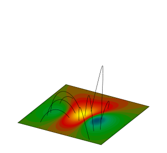
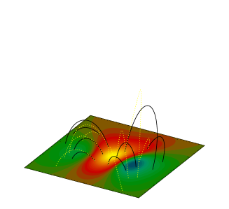
Figure 3 top right panel shows that the field lines of a potential field reconstruction are clearly different from the original Low and Lou solution. This naturally leads to high values of the functional and large forces after the bottom boundary has been replaced by the original vector magnetogram. We first apply the optimization code without weighting function . Here the boundaries of the physical domain coincide with the computational boundaries. The lateral and top boundary have the value of the potential field during the iteration. Some low lying field lines are represented quite well (left hand picture in figure 3 second row). These field lines close to the box center are of course close to the bottom boundary and far away from the other boundaries. The (observed) bottom boundary has a higher influence on the field here than the potential lateral and top boundary. Other field lines, especially high reaching field lines deviate from the analytic solution (yellow dotted line).
The values and provide a quantitative measure of the quality of the reconstructed magnetic field in the physical domain. High values correspond to a significant deviation from the force-free state. We applied the method of boundary relaxation (marked with b.r. in table 1), but the result only slightly improved 222The boundary relaxation method uses the iterative improvement for fields on the lateral and top boundary with as in (18) in addition to (19) with . See ([Wiegelmann and Neukirch (2003)] section 4.2.3 for details..
We investigate how the size and shape of a boundary layer influences the quality of the reconstruction. Both the comparison of the field lines (figure 3 panel 4 to 6) as well as the quantitative values in table 1 show that the quality of the reconstruction improves significantly with the size of the boundary layer (thickness in number of grid points ). The larger computational box displaces the lateral and top boundary further away from the physical domain and consequently its influence on the solution decreases. As a result the magnetic field in the physical domain is dominated by the vector magnetogram data, which is exactly what is required. We find that a cos-profile of the weighting function provides the best results, followed closely by a tanh-profile. The main advantage of these profiles seem to be that they have smooth gradients at the boundary of the physical domain to the boundary layer as well as at the boundaries of the computational box. We tried also a homogenous profile ( in the whole computational box, marked with hom in table 1). In the homogeneous case is equal in the whole computational box and a boundary layer does not exist. The use of for the homogeneous case in table 1 is only for diagnostic reasons and indicates that and have been computed in the same interior box (physical domain) as in the cases with weighting function for comparison. The effect that the lateral and top boundary are far away from the physical domain remains valid here, but the use of a weighting function in the boundary layers provides much better results.
4.1.1 The influence of noise
The previous calculations have been carried out under the assumption that the magnetic field on the boundary of the computational box is known exactly. Such an idealized situation will not be found when real vector magnetogram data are used. To keep control over the amount of uncertainty, we have carried out test runs by adding random noise to the vector magnetogram. We add the noise by multiplying the exact boundary conditions with a number where is a random number in the range and is the noise level. We investigate the effect of noise for Force-Free I with a boundary layer of grid points and a cos profile in for different noise levels.


| noise level | |||
|---|---|---|---|
| no noise | |||
Table 2 and figure 4 show our results. , and increase linearly with the noise level. The field line pictures in the upper panel of figure 4 show that low lying field lines are represented almost correctly while there are some deviations from the analytic Low and Lou solution for high reaching field lines. As the noise is completely random and independent between neighbouring grid points there are obvious difficulties regrading the discretisation. Our code uses forth order finite differences and consequently five grid points are required to compute derivatives. The highly oscillatory noise (The spatial variation of the noise corresponds to the spatial resolution of the grid.) naturally results in finite gradients which are linearly dependent from the noise level. is linearly dependent from spatial deviations and does consequently also depend linearly on the noise level. The computation of and contain gradients squared and are consequently quadratic dependent from the noise level. A pre-processing of raw magnetogram data, e.g. a Fourier filter or some smoothing might help to reduce the effect of random noise.
As the weighting function is designed to diminish the effect of the lateral and top boundary towards the solution, we investigate here how changes on these boundaries influence the solution. We undertook (for and a cos-profile) two runs with linear force free magnetic fields ( and ) on the lateral and top boundaries. , and are of the same order as for potential boundary conditions: potential : , , : , , : , ,
The magnetic field lines calculated from these fields look exactly the same as for potential boundary conditions. We conclude that the influence of the lateral and top boundary conditions towards the solution in the physical domain is indeed very small.
4.2 Force-Free II
The magnetogram on the right hand side of figure 2 is obviously bad conditioned. Significant parts of the magnetic flux are outside of the framed physical domain. In principle it would be better to always choose a magnetogram such that the majority of the flux is centered and the overall flux is approximately balanced but due to the limited size of vector magnetograms sometimes vector magnetograph data are not available over an entire active region. Here we investigate how this influences the quality of the reconstruction. We find that the reconstruction without weighting function provides much worse results in such a case than for a well centered force-free configuration. This is obvious caused by the potential field assumed on the lateral boundary in a region of a high magnetic flux and current density. The influence of the inconsistent lateral boundary conditions on the magnetic field in the physical domain is too strong. Here the method of boundary relaxation improves the quality of nearly by a factor of two, but the result still remains unsatisfactory. For runs with weighting function the result is basically similar as for Force-Free I. A large boundary layer (now including all active parts of the magnetogram) improves the quality of the reconstruction significantly. For the largest boundary layer points wide the quality of the reconstruction is approximately equal to a point wide boundary layer in the Force-Free I case.
If for observational data only parts of an active region are available as vector magnetogram data a nonlinear reconstruction of the coronal magnetic field might become difficult or impossible. One could try to get the corresponding normal component of the photospheric magnetic field from other sources, e.g. the line of sight magnetograph MDI on SOHO and make assumptions regarding the transversal magnetic field. The reconstructed magnetic field will then of course be influenced by these (not observed) assumptions.
5 Tests for non force-free configurations

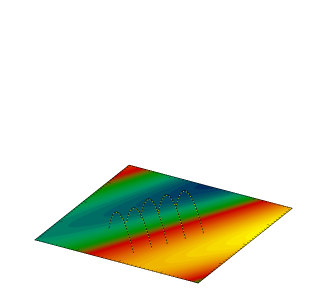
For finite configurations it is necessary to include pressure and gravity forces and solve the magneto hydro static equations (4)-(6). To test our code we use an analytic MHS equilibrium (see [Wiegelmann and Inhester (2003)] section 3.1.) with an average plasma . From this analytic solution we extract a photospheric vector magnetogram and the coronal density distribution. It is convenient to use the analytic density distribution here to test our code, but one has to keep in mind that for observational data the coronal density structure has to be reconstructed with help of a tomographic inversion. Corresponding observational data (line of sight integrals of the coronal density structure) are expected from the Stereo-mission. The tomographic inversion of these data is a challenging problem on its own and we are not going to discuss it here. [Wiegelmann and Inhester (2003)] give an overview over the tomographic inversion algorithm. Here we consider the vector magnetogram and the plasma density distribution as given. The left hand panel of figure 5 shows a potential magnetic field reconstruction consistent with the normal component of the magnetic field extracted from an analytic magneto hydro static equilibrium. The comparison of the magnetic field lines of the potential field with the exact field show significant deviations. In table 1 we diagnose and similarly as for the force-free cases and we diagnose the force balance here. Similar as in the force-free case we find that the quality of the reconstruction is poor for an optimization without weighting function. A boundary layer of points together with a cos-profile of improves the value of functional by a factor of in the physical domain and the force balance 333The functional contains the square of the force balance, see the definition 13. by a factor of about . In the right hand panel of figure 5 we compare the reconstructed field with the analytic solution and both coincide within the graphical resolution. A larger boundary layer of further improves the quantitative measures of the non force-free reconstruction. The influence of a weighting function acts similarly for force-free and non force-free configuration. In both cases the reconstruction result is significantly improved.
6 Conclusions
In this paper we improved the optimization method for the reconstruction of non linear force-free and not force-free coronal magnetic fields. The optimization method minimizes a functional which consists of a quadratic form of the force balance and the solenoidal condition. While in previous optimization attempts the magnetic field needed to be described on all six boundaries of a computational box, our approach allows us to reconstruct the coronal magnetic field from the bottom boundary data alone. This is possible by the introduction of a boundary layer around the physical domain. The physical domain is a cubic area within which we want to reconstruct the coronal magnetic field consistent with photospheric vector magnetogram data. The boundary layer replaces the hard lateral and top boundary used previously. We showed that the limit of an infinitesimally thin boundary layer formally coincides with the original hard boundary. However, our test calculations show that a finite size weighted boundary yield much better results.
We introduced a weighting function. In the physical domain the weighting function is unity. It drops monotonically in the boundary layer and reaches zero at the boundary of the computational box. At the boundary of the computational box we set the field to the value of the potential field computed from at the bottom boundary. This choice is not only convenient due to its mathematic simplicity, but as well physical motivated. The coronal magnetic field is approaching a potential field in quite regions and high in the corona. The current program uses a cartesian geometry and is designed to reconstruct basically isolated active regions. The photospheric magnetic field outside this active region (and a surrounding area) is ignored. This approach is the better justified the more the active region is isolated. Often, however, active regions are not always completely isolated but magnetically connected with other active regions. To include this effect it would in principle be preferable to reconstruct the complete coronal magnetic field with vector magnetogram data on the whole photosphere as boundary. This would avoid the problems of prescribing the lateral boundaries and only the top boundary has to be chosen accordingly, similar to the source surface of potential field reconstructions. We do not expect any difficulties to apply our method to problems in spherical geometry. Unfortunately the required photospheric boundary data are not available because current vector magnetographs do not observe the entire solar surface. The situation will probably significantly improved by the vector spectromagnetograph of the the SOLIS project. It will deliver full disk vector magnetograms.
Acknowledgements.
We thank Bernd Inhester for useful discussions. This work was supported by DLR-grant 50 OC 0007. We thank the referee Thomas R. Metcalf for useful remarks.Appendix A Derivation of and in (14).
| (A.1) |
| (A.2) |
We vary L with respect to an iteration parameter t and get
| (A.3) | |||||
Our aim is now to use vector identities and Gauss law in such way that all terms contain a product with . This will allow us to provide explicit evolution equations for to minimize . The third term has the correct form already. We expand the first and second term
| (A.4) | |||||
The fourth and fifth term have the correct form. We apply the vector identities to the first and second term
| (A.5) | |||||
Term two, four and five have the correct form. We apply to term 1 and to term 3
| (A.6) | |||||
Until here the derivation has been identical with the method without weighting function [Wiegelmann and Inhester (2003)]. Now we get additional terms with respect to the weighting function. We apply to term 2 and 5
| (A.7) | |||||
The terms 1,4,5,7,8 and 9 have the correct form. We apply Gauss’ law to term 2 and 6
| (A.8) | |||||
Now all terms except the terms 2 and 3 have the correct form. We apply to term 2 and 3
| (A.9) | |||||
Now all terms have the correct form and we write them more compact
| (A.10) |
| (A.11) | |||||
| (A.12) |
| (A.13) | |||||
| (A.14) |
References
- Aly (1989) Aly, J.J.: 1989, Solar Phys. 120, 19-48.
- Amari et al. (1997) Amari, T., Aly, J.J., Luciani, J.F., Boulmezaoud, T.Z., Mikic, Z.: 1997, Solar Phys. 174, 129.
- (3) Amari, T., Boulmezaoud, T. Z., and Mikic, Z.: 1999, Astron. Astrophys., 350, 1051-1059.
- Arnaud and Newkirk (1987) Arnaud, J. and Newkirk, Jr.G.: 1987, Astron, Astrophys., 178,263-268
- Berger (1984) Berger, M.A.:1984, Geophys. Astrophys. Fluid Dynamics, 30,79-104
- Carcedo et al. (2003) Carcedo, L., Brown, D.S., Hood, A.W., Neukirch, T., Wiegelmann, T.: 2003 Solar Phys. accepted
- Chiu and Hilton (1977) Chiu, Y.T., Hilton, H.H.: 1977, Astrophys. J. 212, 821.
- Chodura and Schlüter (1981) Chodura, R., and Schlüter, A.: 1981 J. Comp. Phys. , 41, 68-88.
- Gary (2001) Gary, G. A.: 2001, Solar Phys., 203, 71-86.
- House (1977) House, L.L.:1977 Astrophys. J., 214. 632-652
- Judge (1998) Judge, P.G.:1998 Astrophys. J., 500. 1009-1022
- Judge et al. (2001) Judge, P.G., Casini, R., Tomczyk, S., Edwards, D.P. and Francis, E.: 2001, Coronal magnetometry: a feasibility study, NCAR/TN-466+STR, NCAR technical note
- Louis (1989) Louis, A.K.: 1989, Inverse und schlecht gestellte Probleme, Teubner Studienbuecher ISBN 3-519-02085-X.
- Low and Lou (1989) Low, B.C. and Lou, Y.Q.: 1989 Astrophys. J., 352, 343-352.
- Metcalf (1994) Metcalf, T.R.: 1994 Solar Phys., 155, 235-242.
- Petrie and Neukirch (2000) Petrie, G.J.D. and Neukirch, T.: 2000, Astron. Astrophys. 356, 735.
- Roumeliotis (1996) Roumeliotis, G.: 1996, Astrophys. J., 473, 1095-1103.
- Sakurai (1981) Sakurai, T.: 1981, Solar Phys. 69, 343.
- Schmidt (1964) Schmidt, H.V.: 1964 in W.N. Ness (ed.), ASS-NASA Symposium on the Physics of Solar Flares, NASA SP-50, p. 107.
- Seehafer (1978) Seehafer, N.: 1978, Solar Phys., 58, 215.
- Seehafer (1982) Seehafer, N.: 1982, Solar Phys., 81, 69-80
- Semel (1967) Semel, M.: 1967, Ann. Astrophys. 30, 513.
- Semel (1988) Semel, M.: 1988, Astron. Astrophys. 198, 293.
- Wheatland et al. (2000) Wheatland, M. S., Sturrock, P. A., and Roumeliotis, G.: 2000, Astrophys. J., 540, 1150-1155.
- Wiegelmann and Neukirch (2002) Wiegelmann, T. and Neukirch, T.: 2002 Solar Phys., 208, 233-251.
- Wiegelmann and Neukirch (2003) Wiegelmann, T. and Neukirch, T.: 2003, Nonlinear Processes in Geophysics, 10, 313-322
- Wiegelmann and Inhester (2003) Wiegelmann, T. and Inhester, B.: 2003, Solar Phys., 214, 287-312.
- Wu et al. (1990) Wu, S. T., Sun, M. T., Chang, H. M., Hagyard, M. J., and Gary, G. A.: 1990 Astrophys. J., 362, 698-708.