Similarities and differences between coronal holes and the quiet Sun: are loop statistics the key?

Abstract

Coronal holes (CH) emit significantly less at coronal temperatures than quiet Sun regions (QS), but can hardly be distinguished in most chromospheric and lower transition region lines. A key quantity for the understanding of this phenomenon is the magnetic field. We use data from SOHO/MDI to reconstruct the magnetic field in coronal holes and the quiet Sun with the help of a potential magnetic model. Starting from a regular grid on the solar surface we then trace field lines, which provide the overall geometry of the 3D magnetic field structure. We distinguish between open and closed field lines, with the closed field lines being assumed to represent magnetic loops. We then try to compute some properties of coronal loops. The loops in the CH are found to be on average flatter than in the QS. High and long closed loops are extremely rare, whereas short and low-lying loops are almost as abundant in coronal holes as in the quiet Sun. When interpreted in the light of loop scaling laws this result suggests an explanation for the relatively strong chromospheric and transition region emission (many low-lying, short loops), but the weak coronal emission (few high and long loops) in coronal holes. In spite of this contrast our calculations also suggest that a significant fraction of the cool emission in CHs comes from the open flux regions. Despite these insights provided by the magnetic field line statistics further work is needed to obtain a definite answer to the question if loop statistics explain the differences between coronal holes and the quiet Sun.

Appl. Opt. Kluwer Prepress Department
P.O. Box 990
3300 AZ Dordrecht
The Netherlands

KAPKluwer Academic Publishers; compuscriptElectronically submitted article

KAPKluwer Academic Publishers; compuscriptElectronically submitted article

D24, L60, 047

1 Introduction

Coronal holes [Waldmeier (1957), Waldmeier (1975)], are regions with a significantly reduced emissivity in lines corresponding to coronal temperatures. Usually coronal holes are divided into two classes. During solar activity minimum large polar coronal holes exist with opposite magnetic polarity in the northern and southern hemisphere. Around solar activity maximum smaller isolated coronal holes are present at different latitudes, even close to the equator. However, the main property of coronal holes, the reduction in brightness of coronal radiation is common to both types. For the rest of the paper we distinguish between quiet Sun regions without coronal holes (and call them simply Quiet Sun regions QS) and quiet Sun regions inside coronal holes (which we call Coronal holes CH).

An intriguing observation is that the emission from chromospheric and transition region lines formed at temperatures below $6\;10^{5}K$ is not significantly reduced in coronal holes [Wilhelm et al. (2000), Stucki et al. (2000), Stucki et al. (2002), Xia (2003)] with the exception of He lines, whose formation is strongly affected by coronal radiation. Here we use a simple statistical analysis of the magnetic structure to see if a cause for this behaviour can be found, viz. that coronal holes can easily be identified in radiation alone at $10^{6}K$, but are not seen below $6\;10^{5}K$.

Coronal holes are also visible in absorption lines. The $1083$ absorption line in He I is very useful for the identification of coronal holes, because it has a greatly reduced absorption there [Harvey et al. (1975)] and this line has the additional advantage that it can be observed from the ground. The coronal maps used in this paper (see Figs. 1 and 2) have been created at NSO/Kitt Peak from these He I observations [Harvey and Recely (2001)].

The key quantity for the understanding of coronal holes is the magnetic field. According to current understanding coronal holes differ from the normal quiet Sun mainly through the structure of the magnetic field, with the field lines being mainly closed in the normal quiet Sun and open above coronal holes (e.g. Altschuler et al. 1972). Hot gas is trapped in closed loops, but is able to escape along the open field lines. The trapped gas radiates, causing the normal quiet Sun to be brighter.

Although this basic difference in magnetic structure can qualitatively explain the decreased coronal brightness in coronal holes, it begs the question why transition region brightness is not different as well. One possibility is that the chromospheric and transition region are located near the footpoints of the magnetic field lines and their properties are independent of the properties of the overlying corona. One argument against this idea come from the fact that in such a model the transition region is heated by downward conduction of heat from the corona. If there is significantly less coronal gas, as in a coronal hole it is surprising that the transition region is not affected. Another problem with such models was pointed out by, e.g., dowdy86. The emission measure predicted by models such as that of Gabriel (1976) falls far short of the observations at lower temperatures. dowdy86 proposed that short, cool loops are common in the quiet Sun. They harbour a significant fraction of the gas at lower transition region temperatures. Evidence for such loops has been found by Feldman (1998; 2001).

Since the temperature of a loop depends on its length $(T\propto L^{1/3})$; Rosner, Tucker and Vaiana (1978), Kano and Tsuneta (1996) short loops are expected to be cool, while long loops are expected to be hot. Thus, one way of explaining the decreased coronal emission together with the unaffected transition region emission in coronal holes is by having a greatly decreased number of long loops, but an almost equal number of short loops relative to the normal quiet Sun. Here we test this hypothesis.

The magnetic field strength in the photosphere beneath coronal holes has been measured by several authors, (e.g., Levine 1977, Bohlin and Sheeley 1978, Harvey et al. 1982, DeForest et al. 1997, Belenko 2001). The magnetic flux in coronal holes clearly shows a dominant polarity. This is consistent with coronal holes being the source region of the fast solar wind flowing on open magnetic field lines. harvey82 found an average magnetic field strength in coronal holes of 3 to 36 G near the solar activity maximum and 1 to 7 G close to the minimum. Zhang et al. (2002; 2003) found a range from about 4 to 30 G, where polar coronal holes are more close to the lower and solar maximum coronal holes more close to the higher limit of this range. The magnetic field is, however, not exclusively unipolar in coronal holes and consequently coronal holes should contain also locally closed coronal loops besides the open flux Levine (1977).

The presence of both magnetic polarities inside the coronal hole leads to the formation of closed magnetic loops. Here we compare features of these closed loops in coronal holes with quiet Sun loops by extrapolating the magnetic field starting from photospheric magnetograms. We organize the paper as follows. In section 2 we describe the method for computing the magnetic field from photospheric magnetograms. In section 3 we compare the average height and length of magnetic loops for several coronal holes and quiet Sun regions. The distribution functions of loop length and heights are investigated in section 4, while in section 5 we compute loop temperatures with the help of scaling laws. In section 6 we discuss which magnetic features are responsible for coronal holes and finally we draw conclusions and give an outlook for future work in section 7.

2 Reconstruction of the magnetic field in the solar atmosphere

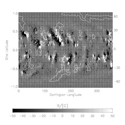
Figure 1: A synoptic chart (09.04.2001-06.05.2001) of the magnetic field constructed from SOHO/MDI. The boundaries of coronal holes taken from He I measurements made at Kitt Peak are overlaid. The analysed coronal holes are numbered.

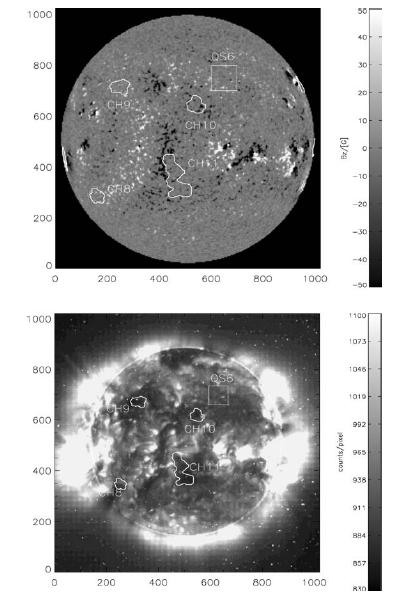
Figure 2: Full disk MDI magnetogram (top panel) and EIT Fe XII, $19.5nm$ image (bottom panel) for 16.4.2001 at 02:30h, with boundaries of coronal holes overlaid. Also marked is an analysed quiet Sun region. The disc center corresponds to a Carrington longitude of $272^{\circ}$.

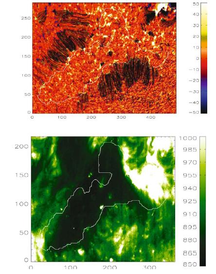
Figure 3: Top panel: MDI magnetogram (colour) with overlaid (black) closed magnetic loops in a coronal holes and the neighbouring quiet Sun. We only plot field lines with a magnetic field strength $B_{\rm lim}\geq 20G$ in order to allow individual loops to be distinguished. In the actual calculations a lower threshold of $2.7G$ is used. The coronal hole is outlined in white. Bottom panel: EIT $19.5nm$ image of the same region. Both images show the number of pixels on the x and y axis. Please note the different pixel size of MDI ($1pixel=1.978arcsec$) and EIT ($1pixel=2.629arcsec$).

Direct measurements of the magnetic field in the chromosphere and corona are mainly restricted to large active regions (e.g. Kundu et al. 2001, White 2002, Solanki et al. 2003, Lagg et al. 2004), although a few measurements of the magnetic field in the quiet corona are available (e.g. Lin et al. 1998, Raouafi et al. 2002). This kind of data is only available for a few individual cases and usually one has to calculate the coronal magnetic field by means of an extrapolation from photospheric field measurements. The extrapolation method requires some assumption regarding electric currents in the solar atmosphere. The simplest approach is to compute current free or potential magnetic fields (e.g. Schmidt 1964, Semel 1967). Potential fields can be reconstructed from the line of sight photospheric magnetic field alone. The corresponding photospheric magnetic field measurements are available e.g. from the SOHO/MDI line-of-sight magnetograph Scherrer et al. (1995). Force free and non-force-free magnetic field models are mathematically more difficult and need additional observational data, e.g. photospheric vector magnetic fields, optical observation of coronal plasma structures or even, additionally, the tomographicly reconstructed density structure for non-force-free configurations. For low lying loops in the quiet Sun investigated in this work we concentrate on potential fields. Coronal currents have a significant effect on the structure of long (say, some $100Mm$ long) loops in active regions, but for the very short (some $10Mm$ or less) quiet Sun loops investigated here their influence can be neglected.

We use a Greens function method to compute the potential magnetic field in the solar atmosphere (see Aly 1989, and appendix A for details.) We investigated $12$ coronal hole and $8$ quiet Sun regions during Carrington rotation 1975 (09.4.-06.05.2001). This period was employed because 56 consecutive 1-min magnetograms are available every day, from which 56 min averages are constructed, after compensating for solar (differential) rotation (see Krivova and Solanki 2004). The magnetic field data were taken from full disc MDI magnetograms when the coronal hole was closest to the central meridian (See table 2 in appendix A). As an example, we show the potential magnetic field lines for coronal hole region 7 and the surrounding area in figure 3, top panel. The image displays only the closed loops with a lower limit of the magnetic field strength $20G$. Open field lines are not shown. Outside the coronal hole (thick white line) the loop density is significantly higher and the loops are also longer than in the hole. The bottom panel of figure 3 shows the same region in the EIT Fe XII $19.5nm$ line. In the coronal hole both the emissivity in EIT as well as the number and length of coronal loops are significantly reduced, although in the rightmost and bottom left edges extended bright structures are found within the CH boundary determined from 1083 He I observations.

A crucial step is how to draw conclusions about the properties of coronal loops from magnetic field lines. Due to the high conductivity the coronal plasma is frozen into the magnetic field. Consequently the emitting plasma structures also outline the magnetic field lines. The gradients of e.g. the plasma pressure and temperature perpendicular to the magnetic field are much higher than along the magnetic field. Within the statistical study it is assumed that these properties are constant along a given field line and only changes from one bundle of field lines to the next. This assumption seems to be not so bad and is consistent with CDS observations regarding the thermal structure of hot coronal loops Brkovic et al. (2002). Theoretically the number of magnetic field lines in the corona (and even the number of field lines in one observed plasma loop) is infinite. To undertake statistical studies regarding the length and height of coronal loops we make the following assumptions. Each magnetic field line starts at the center of a MDI pixel. We assume that this field line is representative for all magnetic field lines starting within the area of the corresponding MDI pixel on the photosphere. Each such representative closed field line is assumed to also represent a magnetic loop. Consequently the number of magnetic loops is determined by the fraction of MDI-pixels that correspond to closed field lines. Now, it can be argued that this is an arbitrary measure of a loop. This is true, but given that from an extrapolation of the magnetic field alone no conclusions can be drawn regarding the distribution of the coronal plasma transverse to the field lines, this is a reasonable assumption. An MDI pixel is the smallest spatial scale which is accessible to us for the extrapolation and the assumption that each pixel supports a separate loop is driven by the small-scale structure seen by TRACE and the NIXT instrument (e.g. Golub et al. 1990). Although individual plasma loops may well be formed from field lines gathered from different sized areas on the solar surface, our approach should in a statistic sense provide the correct distribution of loop lengths, heights, etc. A bias could be introduced into the comparison between quiet Sun and coronal hole only if on average loops in one of these regions are thicker than in the other, for which we have found no evidence in the literature.

3 Analysis of loop height and length

Table 1: Table of coronal holes (CH) and quiet Sun regions (QS). The first column identifies the region, the second column shows the spatially averaged net magnetic field $\langle B_{z}\rangle$ in $G$, the third column the relative flux balance $\frac{\langle B_{z}\rangle}{\langle|Bz|\rangle}$, the fourth column the area of the analysed feature, the fifth column the average height $H$ (in Mm) of closed loops, the sixth column the average length $L$ of closed loops (in Mm), the second last column the number $n$ of closed loops and the last column the density of loops. CH1* and QS3* are not included in the further analysis. Unsigned values have been used when forming the average (excluding CH1 and QS3).

	$\frac{\langle B_{z}\rangle}{[G]}$	$\frac{\langle B_{z}\rangle}{\langle|B_{z}|\rangle}$	$\frac{Area}{Mm^{2}}$	$\frac{H}{[Mm]}$	$\frac{L}{[Mm]}$	$n$	$\frac{n}{Area}$
CH1*	$-0.8$	$-0.25$	$7497$	$3.7$	$20.8$	911	$0.12$
CH2	$-7.9$	$-0.82$	$25071$	$0.7$	$7.0$	2009	$0.08$
CH3	$-14.3$	$-0.91$	$16863$	$1.7$	$17.6$	949	$0.06$
CH4	$8.3$	$0.90$	$14435$	$0.5$	$4.0$	607	$0.04$
CH5	$2.7$	$0.62$	$19471$	$0.9$	$7.1$	1594	$0.08$
CH6	$17.2$	$0.95$	$7998$	$0.7$	$10.8$	310	$0.04$
CH7	$3.7$	$0.58$	$65077$	$0.8$	$5.2$	9199	$0.14$
CH8	$8.8$	$0.83$	$7117$	$0.5$	$3.7$	574	$0.08$
CH9	$2.2$	$0.59$	$7189$	$1.6$	$9.7$	552	$0.08$
CH10	$-6.8$	$-0.86$	$6049$	$0.8$	$6.4$	271	$0.04$
CH11	$-3.0$	$-0.59$	$17895$	$0.8$	$6.6$	1866	$0.10$
CH12	$8.8$	$0.78$	$4349$	$0.6$	$7.6$	253	$0.06$
$\langle\mbox{CH}\rangle$	$7.6$	$0.77$	$17410$	$0.9$	$7.8$	$1650$	$0.07$
QS1	$-0.1$	$-0.02$	$43904$	$3.0$	$15.1$	10122	$0.23$
QS2	$0.5$	$0.10$	$15876$	$4.3$	$22.0$	2653	$0.17$
QS3*	$-4.3$	$-0.62$	$37632$	$0.9$	$6.4$	5815	$0.15$
QS4	$-0.1$	$-0.02$	$7056$	$3.1$	$13.5$	914	$0.13$
QS5	$1.2$	$0.29$	$7056$	$2.5$	$11.4$	1129	$0.16$
QS6	$0.3$	$0.09$	$7056$	$3.3$	$15.2$	1254	$0.18$
QS7	$0.4$	$0.07$	$11760$	$2.3$	$9.2$	3580	$0.30$
QS8	$-0.1$	$-0.03$	$7056$	$2.8$	$12.6$	1382	$0.20$
$\langle\mbox{QS}\rangle$	$0.4$	$0.09$	$14252$	$3.0$	$14.1$	$3005$	0.20

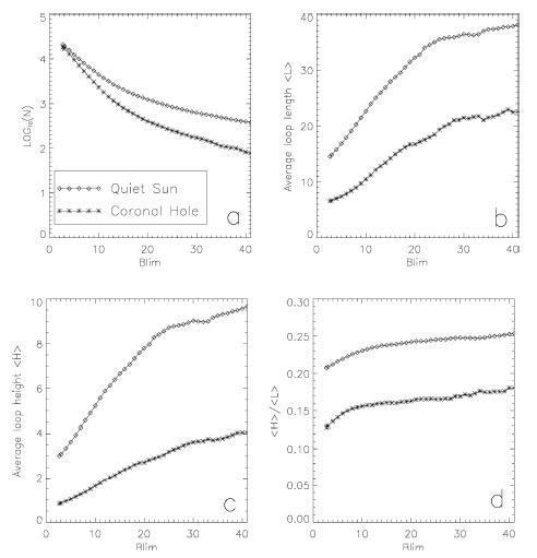
Figure 4: a: The total number of loops, logarithmic scaling, b: the average loop length c: the average loop height d: the ratio of average height to length vs. the minimum magnetic flux $|B_{\rm lim}|/[G]$ considered. The rhombi correspond to quiet Sun regions and the stars to coronal hole regions in all panels.

In table 1 we present some magnetic properties of the analysed coronal holes and quiet Sun regions. In coronal holes the average field strength of the net magnetic flux $\langle B_{z}\rangle$ is usually higher than in the quiet Sun and the ratio of net unsigned magnetic field strength $\frac{\langle B_{z}\rangle}{\langle|Bz|\rangle}$ is higher in coronal holes as well. $\langle B_{z}\rangle$ for CHs is above $2.5$ and $\frac{\langle B_{z}\rangle}{\langle|Bz|\rangle}>0.5$, while for the QS regions these quantities are below $1.2$ and $0.3$, respectively.

An exception is CH1, which shows untypical features for all quantities compared with the other coronal hole regions, and appears to have properties more similar to quiet Sun regions. Another is the quiet Sun region $QS3$ which shows typical coronal hole features. We expect that these regions have been misidentified and do not consider CH1 and QS3 for the statistical investigations in the following. Without these two regions the average values of
$\langle B_{z}\rangle$ and $\frac{\langle B_{z}\rangle}{\langle|Bz|\rangle}$ are $7.6{{}^{+}_{-}}4.8$ and $0.77{{}^{+}_{-}}0.14$ in CHs and $0.4{{}^{+}_{-}}0.4$ and $0.09{{}^{+}_{-}}0.09$ in the QS, respectively.
The unbalanced flux in coronal holes (on average $77\%$) leads to open field lines and to the absence of long closed field line structures as we shall see below.

The most striking feature of table 1 is that the average height and length of loops is significantly smaller in coronal holes compared with the quiet Sun. To compute average values of loop length and height for all quiet Sun and coronal hole regions there are two possibilities. We compute a large number of loops from an equidistant grid of foot-points and give each loop in different regions the same weight. This leads to an average loop length and height of
$\langle H_{CH}\rangle=0.84Mm$, $\;\langle L_{CH}\rangle=6.56Mm$ in CHs ($18184$ loops) and $\langle H_{QS}\rangle=3.02Mm$, $\;\langle L_{QS}\rangle=14.53Mm$ in QS ($21034$ loops).
In these statistics large regions (with many loops) obtain a higher weight than small regions (e.g. CH7 contains about half of all coronal hole loops). Another possibility is to give each region the same statistical weight and average over $\langle H\rangle$ and $\langle L\rangle$ from table 1. This leads to slightly different values:
$\langle H_{CH}\rangle=0.87{{}^{+}_{-}}0.4Mm$, $\;\langle L_{CH}\rangle=7.8{{}^{+}_{-}}3.9Mm$ in CHs and $\langle H_{QS}\rangle=3.04{{}^{+}_{-}}0.7Mm$, $\;\langle L_{QS}\rangle=14.1{{}^{+}_{-}}4.1Mm$ in QS.

We calculated the standard deviation with $11$ (CH2-CH12) coronal holes and $7$ (QS1-QS8, excluding QS3) quiet Sun regions.

The average loop height and length is significantly smaller in coronal holes compared with the quiet Sun. Quiet Sun loops are on average $3.3$ times higher and $1.8$ times longer than coronal hole loops, which means that the average coronal hole loop is not only smaller in size than a quiet Sun loop but also flatter in shape. These averages have been obtained from all loops, independently of the magnetic flux or field strength at their foot points. As the lower limit of magnetic field per pixel we used the effective $1-\sigma$ noise level of $2.7G$ valid for 56-min integrated MDI magnetograms. Since it is not clear whether the residual noise present above the $1-\sigma$ level affects the above results, we investigated how these values change if we consider only closed loops above a certain limit $B_{\rm lim}$ on the statistics. This rules out loops with low magnetic flux $|B|<B_{\rm lim}$. The results are shown in Fig. 4. The number of loops (shown with logarithmic scaling) decreases, as expected, but the decrease is much more significant for coronal hole loops (stars) than for quiet Sun loops (rhombi). This suggest a lack of high flux closed loops in coronal holes and is consistent with the fact that most of the coronal hole flux, in particular in the stronger network elements, is stored in open magnetic fields. (This point will be analysed in greater detail in a separate paper.) The average loop length and height increase with increasing $B_{\rm lim}$, which means that, on average, short and low closed loops have at least one footpoint in regions of low magnetic flux.

The result that closed loops are lower and smaller in coronal holes remains valid independently of whether we consider only loops which contain large magnetic flux or all loops. In fact, the difference in length and height between loops in coronal holes and quiet Sun regions increases with $B_{\rm lim}$. The result that coronal hole loops are on average flatter than quiet Sun loops also remains valid independently of $B_{\rm lim}$. The quotient $\frac{H}{L}$ increases slightly both in coronal holes and the quiet Sun. This implies that loops starting from weak-field regions are a bit flatter. This test shows that the results obtained so far are robust as far as noise in the magnetograms is concerned.

4 Distribution functions for loop height and length

Figure 5: a: distribution function $f(H)$ of loop height. b: distribution function $f(L)$ of loop length. The solid lines correspond to coronal holes and the dotted lines to quiet Sun regions. The error bars have been calculated from the individual statistics of the different coronal hole and quiet Sun regions. c: distribution function $f(H)$ of loop height (solid lines), an exponential fit (dotted lines) and a power law fit (dashed lines) are superimposed on each observed distribution. d: distribution function $f(L)$ of loop length (solid lines), with exponential (dotted lines) and power law fits (dashed lines) superimposed.

In the previous section we investigated the average height and length of closed coronal loops in the quiet Sun and in coronal holes. Here we calculate the distribution functions for the length and height of coronal loops (18184 loops in 11 coronal holes and 21034 loops in 7 quiet Sun regions). We normalize each distribution function by the area of the investigated region (fourth column in Table 1). Fig. 5a shows the height distribution and 5b the length distribution. The solid lines correspond to coronal holes and the dotted lines to quiet Sun regions. We first computed $H\rightarrow\frac{f(H)}{Area}$ and $L\rightarrow\frac{f(L)}{Area}$ for each coronal hole and quiet Sun region separately. The error bars represent the standard deviation over the 11 coronal hole and 7 quiet Sun regions for each interval in $H$ and $L$ respectively. The number of loops with length below a pixel diameter have not been plotted. The curves show firstly that the number of loops decreases rapidly with increasing height or length of the loops and that there are more loops (per unit area) in quiet Sun regions compared to coronal holes, irrespective of loop length and height.

We fit the average $f(H)$ and $f(L)$ with help of an exponential fit ($f(x)=c\cdot\exp(d\cdot x)$) and a power law fit ($f(x)=a\cdot x^{b}$). The best obtained fits are (see also Fig. 5 c and d where exponential fits are represented by dotted lines and power law fits by dashed lines):

$$f_{CH}(H)= 0.055\cdot\exp(-1.09\cdot H)$$

$$f_{QS}(H)= 0.043\cdot H^{-1.12}$$

$$f_{CH}(L)= 0.010\cdot\exp(-0.16\cdot L)$$

$$f_{QS}(L)= 0.015\cdot\exp(-0.09\cdot L)$$

$$f_{QS}(L)= 0.052\cdot L^{-1.08}$$

The exponential function fits the coronal hole distribution functions $f_{CH}(H)$ and $f_{CH}(L)$ very well and is superior to a power law fit, which has also been plotted for comparison. The quiet Sun distribution for the height $f_{QS}(H)$ is closer to a power law distribution, while $f_{QS}(L)$ is not fit well (towards shorter loops) by either function, even if we neglect the shortest loops, whose number is probably influenced by the limited spatial resolution of MDI. We have therefore given the parameters of both fits.

With increasing height and length of the loops the number of loops decreases, but remains significantly higher in the quiet Sun than in coronal holes. It is instructive to plot the ratio of the distributions in coronal holes and the quiet Sun, $\frac{f_{CH}(L)}{f_{QS}(L)}$ and $\frac{f_{CH}(H)}{f_{QS}(H)}$ (see Figs 6 a and b, respectively).

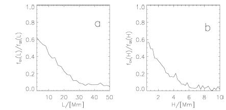
Figure 6: Relative Distribution of loop length ($f_{CH}(L)/f_{QS}(L)$, left panel) and loop height ($f_{CH}(H)/f_{QS}(H)$, right panel). The individual distribution functions have been normalized by the area covered by the solar feature. The distribution functions have been computed using all loops in quiet Sun and coronal hole regions (except CH1 and QS3).

Figure 7: Relation between loop length $L$ and volume $V$ (double logarithmic scaling). The solid gray lines correspond to power law fits. The larger power law exponent obtained for QS (panel a) suggests that these loops expand more than the CH loops of equal length (panel b).

The number of low and short loops in coronal holes is on average about $60\%$ the number of quiet Sun loops. Towards high and long loops this ratio drops rapidly. The number of loops longer than $30Mm$ in coronal holes is only about $5-10\%$ of the number in the quiet Sun. Similarly, the number of loops with a height of around $4Mm$ in coronal holes is only $10\%$ of that in the quiet Sun and the ratio drops further to below $5\%$ for higher loops.

Note that although the number of longer loops drops dramatically in CHs, the volume filled by these loops drops more slowly. We estimate the volume $V$ filled by loops of length $L$ by $V=\int_{0}^{L}\frac{B_{\rm Fp1}}{B(l)}dl\cdot A_{\rm Fp1}$, where $A_{\rm Fp1}$ is the loop cross-section area at one of the foot points, $B_{\rm Fp1}$ the corresponding field strength and $l$ is the distance measured along the loop. The factor $\frac{B_{\rm Fp1}}{B(l)}$ takes into account the expansion of the loop due to magnetic flux conservation. The relation between loop length and volume is shown in figure 7. The solid gray lines are power fits to the determined values. The larger exponent obtained for the quiet Sun suggests that these loops expand more than the CH loops of equal length. This is not surprising given that the CH loops are flatter, i.e. do not reach so high into the atmosphere as equivalent QS loops.

5 Relation of loop length to temperatures.

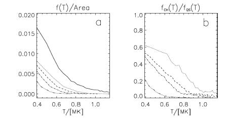
Figure 8: a: Distribution function $T\rightarrow f(T)$ for QS (solid line) and CH, were T is the temperature. We computed the temperature from the loop length with help of the RTV-model $(T\propto(pL)^{1/3}$. The pressure $p$ was chosen $0.11/[dyn\;cm^{-2}]$ on the quiet Sun and $0.11/[dyn\;cm^{-2}]$ (dotted line), $0.08/[dyn\;cm^{-2}]$ (dashed line), $0.055/[dyn\;cm^{-2}]$ (dash-dotted line), $0.03/[dyn\;cm^{-2}]$ (dash-double-dotted line) for coronal holes. (See text). b: Ratio of the distribution of loops as a function of temperature ($f_{CH}(T)/f_{QS}(T)$). The dotted, dash-dotted and dash-double-dotted lines where calculated with the same values of $p$ in the CH as in a).

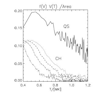
Figure 9: The plot shows $f(V)\cdot V(T)$ normalized to the area of the considered region vs. $T$. The pressure $p$ was chosen $0.11/[dyn\;cm^{-2}]$ on the quiet Sun and $0.11/[dyn\;cm^{-2}]$ (dotted line), $0.08/[dyn\;cm^{-2}]$ (dashed line), $0.055/[dyn\;cm^{-2}]$ (dash-dotted line), $0.03/[dyn\;cm^{-2}]$ (dash-double-dotted line) for coronal holes.

Here we consider in a simple manner implications of the difference in loop statistics for the temperature and temperature distribution in coronal holes. It is not straightforward to draw direct quantitative conclusions regarding the emissivity, however. While one might assume that most of the emission comes from closed magnetic loops, it is likely that some emission is related to open fields. While in quiet Sun regions (where high large loops exist) the emission from open field lines can probably be neglected, this might not be the case for coronal holes. In a region without (or with very few) high and long loops the emission from the dilute plasma on open field lines might become relatively important. The overall emissivity will, of course, still be very small.

In the following we use the assumption that short loops are cooler than long loops. This assumption is supported by a hydrostatic model Rosner, Tucker and Vaiana (1978) (RTV-model) which provides the scaling law

$$T_{max}=1400\cdot(pL)^{1/3},$$ (1)

where $T_{max}$ is the maximum temperature, $L$ the loop length in $cm$ and $p$ the pressure in $dyn\;cm^{-2}$. We use this scaling law to approximate the temperatures of the loops calculated here. We assume that the temperature along the loops equals $T_{\rm max}$. This agrees with the thermal structure of hot loops deduced from CDS (e.g. brkovic02). maxson77 found a pressure of $0.11\;dyn\;cm^{-2}$ for large-scale structures and $0.03\dots 0.08\;dyn\;cm^{-2}$ in coronal holes. Using these scaling laws and $\langle L_{CH}\rangle=7.8\;Mm$ and $\langle L_{QS}\rangle=14.1\;Mm$ we find $\frac{T_{QS}}{T_{CH}}=1.2$ if the pressure is assumed to be the same in coronal holes and the quiet Sun. If the pressure is kept fixed to $0.11$ in the quiet Sun and reduced to $0.08,\;0.055,\;0.03$ (maximum, average and minimum value in coronal holes) we find an increase of the average temperature ratio to $\frac{T_{QS}}{T_{CH}}=1.4,\;1.5\;,1.9,$ respectively. Since the maxson77 values for the CHs refer to high temperatures and probably mix contributions of both open and closed field lines, we suspect that the most realistic result is obtained assuming the pressure in CH loops to be the same as in QS loops. We have neglected any dependence of $p$ on $T$ or $L$.

The effect on the average temperature ratio may not look very dramatic, but the absence of long loops in coronal holes has a dramatic effect on the temperature distribution function, as can be seen from Fig. 8. The number of loops decreases rapidly with temperature for both QS and CH regions, irrespective of the assumed pressure in CH loops. Since longer loops are hotter, the total emitting volume does not as rapidly decrease as suggested by Fig. 8 a).

We find that hot loops are practically absent in coronal holes . The effect is clearly visible already if the same scaling law (same value of $p$)is applied to coronal holes and the quiet Sun. It becomes even stronger when we reduce $p$ in coronal holes following maxson77. Figure 8 (panel b) shows the decrease in the ratio of loops (per area) $\frac{f_{CH}}{f_{QS}}$ with increasing loop temperature. We find that (depending on the assumed $p$) $\frac{f_{CH}}{f_{QS}}$ has a ratio of $0.62,\;0.53,\;0.49,\;0.20$ at a temperature of $0.4MK$ and the ratio reduces to $0.18,\;0.06,\;0.05,\;0.00$ respectively at a temperature of $0.9MK$. Of greater interest for the observations than just the number of loops at a given temperature is the emitting volume filled by gas at that temperature. Using the fits plotted in Fig. 7 we plot $f(V)\cdot V(T)$ normalized to the area of the considered region in figure 9 vs. $T$. Again, the very large contrast at high temperatures and the much smaller contrast at low temperatures are visible.

One has to recognize, however, that the temperatures calculated here with scaling laws can only be a rough estimate. The values of $p$ required for the RTV-model (1) are not know very precisely. In addition, the RTV-model has been derived assuming a static equilibrium (no plasma flow) along the loops, zero gravity, uniform heating and a constant cross section. These assumptions are not exact. Serio et al. 1981 extended the RTV-model, taking into account gravity and non uniform heating. The scaling laws are similar to the RTV-model ($T=1400\cdot(pL)^{1/3}\cdot\exp\left[-0.04L\;\left(2/s_{H}+1/s_{p}\right)\right]$ with the heating deposition scale height $s_{H}$ and the pressure scale height $s_{p}$.) The gravity can probably be neglected here as we deal with loops small compared with the pressure scale height. kano95 showed that the heating deposition distribution along the loop influences the scaling laws. By assuming that the heat input occurs at the top of the loop Kano and Tsuneta 1995 also got the RTV-scaling law (1), but if the heat input is constant along the loop the authors found $T_{\mbox{max}}=1100\cdot(pL)^{1/3}$. If we would use the latter model instead of RTV the loop temperatures would be reduced by a factor of $0.8$. The temperature ratios and the shape of the distribution functions would remain the same, however. Another modification of the RTV-model, e.g. a different loss function Kano and Tsuneta (1995) lead to $T_{\mbox{max}}\propto(pL)^{\gamma}$ with $\gamma$ different from the RTV-value of $1/3$, but these modifications are related to temperatures above $10^{6}K$ and it is not clear to which extent they apply here. aschwanden00 found analytic approximations for hydrostatic loops by fitting results of a numerical code. The authors mainly concentrated on hot ($1-10MK$) loops and the temperature distribution along the loops, which is outside the scope of this paper. winebarger02 have argued that loops are inherently dynamic. Again, such an extension is well beyond the scope of the present paper.

6 What magnetic features are responsible for coronal holes?

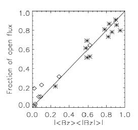
Figure 10: Fraction of open flux, normalized to the total flux of the studied region vs. $\frac{\langle B_{z}\rangle}{\langle|B_{z}|\rangle}$. The correlation coefficient between these quantities is $0.98$. The rhombi correspond to QS and the stars to CH. The solid line corresponds to $\frac{\langle B_{z}\rangle}{\langle|B_{z}|\rangle}=$ fraction of open flux.

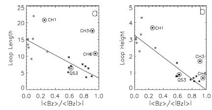
Figure 11: The figure shows the relative net flux $\frac{\langle B_{z}\rangle}{\langle|B_{z}|\rangle}$ against the average loop length (left panel) and average loop height (right panel). Each symbol represents one region. The rhombi correspond to the quiet Sun regions and the stars to coronal holes. The lines are a linear fit (CH1, CH3, CH6 and QS3 are shown in the figures (and marked with circles), but have not been considered for the linear fit.).

From previous publications Harvey et al. (1982); DeForest et al. (1997); Wilhelm (2000); Belenko (2001) we know that the magnetic flux in coronal holes is dominated by one polarity and consequently the magnetic field in a coronal hole is not flux balanced. This result is confirmed by Table 1. On average $\frac{\langle B_{z}\rangle}{\langle|B_{z}|\rangle}=0.77$ for the studied CHs and $\frac{\langle B_{z}\rangle}{\langle|B_{z}|\rangle}=0.09$ for the QS regions. Except for one region each, all CHs are distinctly different from the QS regions.

Here we investigate how $\frac{\langle B_{z}\rangle}{\langle|B_{z}|\rangle}$ is related to the amount of open flux, the average loop length $\langle L\rangle$ and height $\langle H\rangle$.

Figure 10 shows the amount of open flux, normalized to the total flux of the studied region. The rhombi correspond to quiet Sun regions and the stars to coronal holes. (Every rhombus and every star represents one quiet Sun and coronal hole region, respectively.) Remarkably, there is a small scatter (correlation coefficient $0.98$). The reason for the scatter is, that a part of the unbalanced flux in a particular region is closed and connects to fields outside the area entering the statistics (e.g. loops crossing the boundary of the CH.)

Figures 11 a) and b) show the average loop length and the average loop height, respectively, vs. the relative flux balance.

There is a clear trend for the loop height to decrease with $\frac{\langle B_{z}\rangle}{\langle|B_{z}|\rangle}$ , the correlation coefficient between these two quantities being $r_{c}=-0.87$. Interestingly the loop length is not so strongly correlated ($r_{c}=-0.57$), mainly because of CH3 and CH6, which have anomalously long loops (but not strikingly high ones). The strongest correlation is found between $\frac{\langle B_{z}\rangle}{\langle|B_{z}|\rangle}$ and $\frac{\langle H\rangle}{\langle L\rangle}$, the correlation coefficient being $-0.92$. We find that the average unsigned magnetic field strength is about a factor of two higher in coronal holes for the regions investigated here ($\langle|B_{z}|\rangle=9.3{{}^{+}_{-}}4.6G$ in CHs and $\langle|B_{z}|\rangle=4.5{{}^{+}_{-}}0.9G$ in QS).

7 Conlusions

We have investigated the local magnetic field structure of equatorial coronal holes and its relation to the emissivity. Coronal holes have a higher relative background magnetic field than quiet Sun regions and consequently most of the total magnetic flux (usually some $80\%$, for some holes more than $90\%$ and for others only about $60\%$) is unbalanced flux which mainly results in open magnetic field lines. (Some of it may be balanced in nearby regions lying outside the boundary of the CH.)

Closed loops exist, however, also in coronal holes but their average length and height is lower than in the quiet Sun. These results might provide an understanding of the appearance of coronal holes at different wavelength. The number of low and short loops in coronal holes is only somewhat smaller than in the quiet Sun (the ratio being about $65\%$), but for long and high loops the ratio drops to less than $10\%$. We also find that the ratio of loop height to loop length is lower in coronal holes, so that coronal hole loops are flatter. Converting loop length into temperature using the Rosner-Tucker-Vaiana scaling law we obtain that the fraction of the volume filled with transition region gas (at $T=4\,10^{5}K$) in CHs is on average $70\%$ of that in the QS, while at temperatures of $0.9MK$ this fraction drops to $10\%$ (see Fig. 9).

The local magnetic field structure thus provides an explanation why hot coronal line emission is absent in coronal holes. Due to the almost complete absence of closed loops at coronal temperatures in coronal holes there is hardly any emission in lines formed at high temperatures. The current, simple analysis does not provide a full solution of the puzzle yet as why CHs are just as bright as QS at transition region temperatures. Although the volume filling due to cool loops is a large fraction of that in the quiet Sun, it is still significantly lower. This may partly be due to the limited resolution and sensitivity of MDI, so that we underestimate the number of short loops. However, there would still appear to be some need for significant chromospheric and transition region heating along the open field lines in order to reproduce the observations. We must also keep in mind that on average the field is a bit stronger in CHs, so that the open flux need not be quite as bright as the closed, even in TR.

For future work it would be interesting to investigate also the local magnetic field structure of polar coronal holes. Unfortunately, magnetic field measurements of the polar magnetic field are not available to the necessary precision yet. The Solar Orbiter mission Marsch et al. (2001) will provide high quality measurements of polar magnetic fields.

Appendix A The magnetic field model

Table 2: List of coronal hole and quiet Sun regions. The first column stands for the coronal hole CH1-12 and quiet Sun QS1-8 regions investigated. The second and third columns contain the MDI number of the full disk magnetogram and observation date respectively. We chose the full disk magnetograms in order to have the coronal holes closest to the central meridian. The last four columns contain the positions of the investigated region in MDI-pixels.

Region	MDI-N.	Date	xmin	xmax	ymin	ymax
CH1	73058	0503	$406$	$528$	$478$	$572$
CH2	73082	0504	$358$	$613$	$259$	$462$
CH3	73010	0501	$406$	$526$	$457$	$644$
CH4	72962	0429	$425$	$576$	$660$	$815$
CH5	72866	0425	$417$	$632$	$767$	$906$
CH6	72818	0423	$417$	$512$	$369$	$486$
CH7	72842	0424	$260$	$746$	$96$	$385$
CH8	72746	0420	$430$	$560$	$235$	$334$
CH9	72722	0419	$467$	$589$	$668$	$759$
CH10	72650	0416	$491$	$589$	$604$	$695$
CH11	72650	0416	$398$	$542$	$264$	$465$
CH12	72506	0410	$462$	$547$	$676$	$778$
QS1	73058	0503	$500$	$699$	$250$	$429$
QS2	73010	0501	$500$	$629$	$400$	$529$
QS3	72962	0429	$400$	$599$	$220$	$379$
QS4	72818	0423	$450$	$549$	$500$	$599$
QS5	72770	0421	$580$	$679$	$720$	$819$
QS6	72650	0416	$600$	$699$	$700$	$799$
QS7	72842	0424	$470$	$609$	$70$	$169$
QS8	72842	0424	$350$	$449$	$286$	$385$

We use the line of sight magnetic field observed with SOHO/MDI and reconstruct the coronal magnetic field as a potential field with the help of a Greens function method Aly (1989). The potential and magnetic field are presented as

$$\Phi({\bf r}) = -\frac{1}{2\pi}\int_{\partial\Omega}B_{z}({\bf r^{{}^{\prime}}})\,\frac{d\sigma^{{}^{\prime}}}{|{\bf r}-{\bf r^{{}^{\prime}}}|},$$ (A.2)

$${\bf B} = \nabla\Phi,$$ (A.3)

where $\Phi$ is the scalar potential, $B_{z}$ the line of sight photospheric magnetic field, $\partial\Omega$ the bottom boundary (photosphere) of the computational box, $d\sigma=dx\,dy$, ${\bf r}=\sqrt{x^{2}+y^{2}+z^{2}}$ and ${\bf B}$ is the 3D magnetic field.

We use MDI-data as input for our potential magnetic field code. The noise-level of the original MDI-data has been reduced by forming from 56 consecutive 1-min magnetograms, from which 56 min averages are constructed, after compensating for solar (differential) rotation (see krivova04). To avoid the influence of the remaining noise in the magnetic field data, values of $|Bz|<2.7G$ are set to zero, as well as isolated data points (data points with $|Bz|\geq 2.7G$ but with no neighbour points with the same polarity). The resolution of one MDI-pixel is approximately $1.4$Mm. We compute the potential magnetic field in rectangular boxes. The magnetic field lines are calculated with a fourth order Runge-Kutta field line tracer with step size control. The field line tracer interpolates the magnetic field between pixels with a trilinear interpolation routine. The pixel size in our computational box corresponds to one MDI pixel. We start the field line integration on the photosphere and integrated the magnetic field line until it reaches again the photosphere (closed field lines, loops) or the upper boundary of the computational box. These field lines are interpreted as open field lines. This interpretation seems to be quite well justified as the fraction of open flux computed with help of the so defined open field lines and the unbalanced magnetic flux on the photosphere coincide quite well (see figure 10.

To diminish the influence of lateral boundary conditions we do not start the field line integration in a lateral boundary layer of 20 MDI pixels.

References

- Altschuler et al. (1972) Altschuler, Martin D., Trotter, Dorothy E., Orrall, Frank Q.: 1972, Solar Phys. 26, 354-365
- Aly (1989) Aly, J.J.: 1989, Solar Phys. 120, 19-48.
- Aschwanden et al. (2000) Aschwanden, M.J., Nightingale, R.W., Alexander, D.: 2000, ApJ., 541, 1059-1077
- Belenko (2001) Belenko, I.A.: 2001, Solar Physics, 199, 23-35
- Bohlin and Sheeley (1978) Bohlin, J.D. and Sheeley, N.R.Jr.: 1978, Solar Phys.56, 125-151
- Brkovic et al. (2002) Brkovic, A., Landi, E., Landini, M., Rüedi, I., Solanki, S. K.: 2002 Astron. and Astrophys., 383, 661-677
- DeForest et al. (1997) DeForest, C.E., Hoeksema, J.T., Gurman, J.B., Thompson, B.J., Plunkett, S.P., Howard, R., Harrison, R.C., Hassler, D.M.: 1997, Solar Physics, 175, 393-410
- Dowdy et al. (1986) Dowdy, J. F., Jr., Rabin, D., Moore, R. L.: 1986, Solar Phys., 105, 35-45
- Feldman (1998) Feldman, U.: 1998 ApJ., 507, 974-977
- Feldman (2001) Feldman, U., Dammasch, I. E., Wilhelm, K.: 2001 ApJ., 558, 423-427
- Gabriel (1976) Gabriel, A. H.: 1976 Phil. Trans. R. Soc. Lond., A., 281, 339-352.
- Golub et al. (1990) Golub, L., Herant, M., Kalata, K., Lovas, I., Nystrom, G., Pardo, F., Spiller, E., Wilczynski, J.: 1990, Nature, 344, 842
- Harvey et al. (1975) Harvey, J.W., Krieger, A.S., Timothy, A.F., Vaiana, G.S.: 1975, Bull. American Astron. Soc., 7, 358
- Harvey et al. (1982) Harvey, K.L., Sheeley, J.R., Harvey, J.W.: 1982, Solar Physics, 79, 149-160
- Harvey and Recely (2001) Harvey, K.L., Recely, F.: 2001, Coronal hole maps prepared at NSO/Kitt Peak by Karen Harvey and Frank Recely as part of an NSF grant. (http://nsokp.nso.edu/dataarch.html).
- Kano and Tsuneta (1995) Kano, R., Tsuneta, S.: 1995, ApJ, 454, 934-944
- Kano and Tsuneta (1996) Kano, R., Tsuneta, S.: 1996, Publ. of the Astronomical Society of Japan, 48, 535-543
- Krivova and Solanki (2004) Krivova, N. A.; Solanki, S. K.: 2004 Astron. and Astrophys., 417, 1125-1132
- Kundu et al. (2001) Kundu, M. R., White, S. M., Shibasaki, K., Raulin, J.-P.: 2001 ApJ Supplement Series, 133, 467-482
- Lagg et al. (2004) Lagg, A., Woch, J., Krupp, N., Solanki, S.K.: 2004, A & A, 414, 1109-1120
- Levine (1977) Levin, R.H.: 1977, Astrophys. J., 218, 291-305
- Lin et al. (1998) Lin, H., Penn, M.J., Kuhn, J.R.: 1998, ApJ, 493, 978-995
- Maxson and Vaiana (1977) Maxson, C.W., Vaiana, G.S.: 1977 ApJ, 215, 991-941
- Marsch et al. (2001) Marsch, E., Fleck, B., Schwenn, R.: 2001 The Outer Heliosphere: The Next Frontiers, Edited by K. Scherer, Horst Fichtner, Hans Jörg Fahr, and Eckart Marsch COSPAR Colloquiua Series, 11. Amsterdam: Pergamon Press, 2001., p.445
- Raouafi et al. (2002) Raouafi, N.-E., Sahal-Bréchot, S., Lemaire, P.: 2002, Astron. and Astrophys., 396, 1019-1028
- Rosner, Tucker and Vaiana (1978) Rosner,R., Tucker, W.H., Vaiana, G.S.:1978, ApJ., 220, 643-665
- Scherrer et al. (1995) Scherrer, P. H., Bogart, R. S., Bush, R. I., Hoeksema, J. T., Kosovichev, A. G., Schou, J., Rosenberg, W., Springer, L., Tarbell, T. D., Title, A., Wolfson, C. J., Zayer, I., MDI Engineering Team: 1995, Solar Phys. 162, 129-188
- Schmidt (1964) Schmidt, H.V.: 1964 in W.N. Ness (ed.), ASS-NASA Symposium on the Physics of Solar Flares, NASA SP-50, p. 107.
- Semel (1967) Semel, M.: 1967, Ann. Astrophys. 30, 513.
- Serio et al. (1981) Serio, S., Peres, G., Vaiana, G.S., Golub, L., Rosner, R.:1981, ApJ., 243, 288-300
- Solanki et al. (2003) Solanki, S.K., Lagg, A., Woch, J., Krupp, N., Collados, M.: 2003, Nature, 425, 692-695
- Stucki et al. (2000) Stucki, K., Solanki, S. K., Schühle, U., Rüedi, I., Wilhelm, K., Stenflo, J. O., Brkovic, A., Huber, M. C. E.: 2000, Astron. and Astrophys., 363, 1145-1154
- Stucki et al. (2002) Stucki, K., Solanki, S. K., Pike, C. D.; Schühle, U., Rüedi, I., Pauluhn, A., Brkovic, A.:, 2002, Astron. Astrophys. 381, 653-667
- Waldmeier (1957) Waldmeier, M.: Die Sonnenkorona (II). Birkhäuser Verlag Basel und Stuttgart, 1957.
- Waldmeier (1975) Waldmeier, M.: 1975, Solar Phys. 40, 351-358.
- White (2002) White, S.M.: 2002, Astron. Nachr., 323, 265-270
- Wilhelm (2000) Wilhelm, K.: 2000, Astron. Astrophys. 360, 351-362
- Wilhelm et al. (2000) Wilhelm, K., Dammasch, I. E., Marsch, E., Hassler, D. M.: 2000, Astron. Astrophys. 353, 749-756
- Winebarger et al. (2002) Winebarger, A.R., Warren, H., van Ballegooijen, A., DeLuca, E.E., & Golub L. 2002, ApJ., 567, L89
- Xia (2003) Xia, L.: Equatorial Coronal Holes and Their Relation to the High-Speed Solar Wind Streams. PhD-Thesis Göttingen, 2003.
- Zhang et al. (2002) Zhang, J.; Woch, J.; Solanki, S. K.; von Steiger, R.: 2002, GRL 29, pp. 77-1, CiteID 1236, DOI 10.1029/2001GL014471
- Zhang et al. (2003) Zhang, J., Woch, J., Solanki, S. K., von Steiger, R., Forsyth, R: 2003, JGR 108, pp. SSH 1-1, CiteID 1144, DOI 10.1029/2002JA009538