A Time-Evolving 3D Method Dedicated to the Reconstruction of Solar Plumes and Results Using Extreme Ultra-Violet Data

Abstract

An important issue in the tomographic reconstruction of the solar poles is the relatively rapid evolution of the polar plumes. We demonstrate that it is possible to take into account this temporal evolution in the reconstruction. The difficulty of this problem comes from the fact that we want a 4D reconstruction (three spatial dimensions plus time) while we only have 3D data (2D images plus time). To overcome this difficulty, we introduce a model that describes polar plumes as stationary objects whose intensity varies homogeneously with time. This assumption can be physically justified if one accepts the stability of the magnetic structure. This model leads to a bilinear inverse problem. We describe how to extend linear inversion methods to these kinds of problems. Studies of simulations show the reliability of our method. Results for SOHO/EIT data show that we are able to estimate the temporal evolution of polar plumes in order to improve the reconstruction of the solar poles from only one point of view. We expect further improvements from STEREO/EUVI data when the two probes will be separated by about 60^∘.

1 Introduction

A method known as solar rotational tomography has been used to retrieve the 3D geometry of the solar corona (Frazin 2000; Frazin and Janzen 2002). This method assumes the stability of the structures during the time necessary to acquire the data. Since we generally have only one point of view at our disposal, about 15 days are required to have data for half a solar rotation at the poles. Here, we focus our study on solar polar plumes. They are bright, radial, coronal ray structures located at the solar poles in regions of open magnetic field. The study of plumes is of great interest since it may be the key to the understanding of the acceleration of the fast component of the solar wind Teriaca et al. (2003). However the three-dimensional shape of these structures is poorly known and different assumptions have been made, e.g. Gabriel et al. 2005; Llebaria02. The plumes are known to evolve with a characteristic time of approximately 24 hours on spatial scales typical of Extreme ultra-violet Imaging Telescope (SOHO/EIT) data (2400 km) DeForest, Lamy, and Llebaria (2001). Consequently the stability assumption made in rotational tomography fails. Fortunately, the Solar TErestrial RElations Observatory (STEREO) mission consists of two identical spacecraft STEREO${}_{\text{A}}$ and STEREO${}_{\text{B}}$ which take pictures of the Sun from two different points of view. With the SOHO mission still operating, this results in three,simultaneous points of view. Three viewpoints help to improve the reconstruction of the plumes, but they are still not enough to use standard tomographic algorithms. The problem is underdetermined and consequently one has to add a priori information in order to overcome the lack of information. This leads to challenging and innovative signal analysis problems. There are different ways to deal with underdetermination depending on the kind of object to be reconstructed. Interestingly the field of medical imaging faces the same kind of issues. In cardiac reconstruction, authors make use of the motion periodicity in association with a high redundancy of the data Grass et al. (2003); Kachelriess, Ulzheimer, and Kalender (2000). If one can model the motion as an affine transformation, and if one assumes that we know this transformation, one can obtain an analytic solution Ritchie et al. (1996); Roux et al. (2004).

In solar tomography, the proposed innovative approaches involve the use of additional data such as magnetic-field measurements in the photosphere Wiegelmann and Inhester (2003) or data fusion Frazin and Kamalabadi (2005). Attempts have been made by Frazin et al.(2005) to treat temporal evolution using Kalman filtering.

Since polar plumes have apparently a local, rapid, and aperiodic temporal evolution, we developed as in the previously referenced work, a model based on the specifics of the object we intend to reconstruct (preliminary results can be found in Barbey et al.(2007). Plumes have an intensity which evolves rapidly with time, but their position can be considered as constant. This hypothesis is confirmed by previous studies of the plumes such as Deforest01. The model is made up of an invariant morphological part $({\mathb{x}})$ multiplied by a gain term $({\boldsymbol{\theta}}_{t})$ that varies with time. Only one gain term is associated with each plume in order to constrain the model. So we assume that the position of each plume in the scene is known. This model is justified if we consider polar plumes to be slowly evolving magnetic structures in which plasma flows.

Thanks to this model we can perform time-evolving three-dimensional tomography of the solar corona using only extreme ultra-violet images. Furthermore, there is no complex, underlying physical model. The only assumptions are the smoothness of the solution, the area-dependant evolution model, and the knowledge of the plume position. These assumptions allow us to consider a temporal variation of a few days, while assuming only temporal smoothness would limit variations to the order of one solar rotation (about 27 days). To our knowledge, the estimation of the temporal evolution has never been undertaken in tomographic reconstruction of the solar corona.

We first explain our reconstruction method in a Bayesian framework (Section 2). We then test the validity of our algorithm with simulated data (Section 3). An example of a reconstruction on real SOHO/EIT data is shown in Section 4. Results are discussed in Section 5. We conclude in Section 6.

2 Method

Tomographic reconstruction can be seen as an inverse problem, the direct problem being the acquisition of data images knowing the emission volume density of the object (Section 2.1). If the object is evolving during the data acquisition, the inverse problem is highly underdetermined. So our first step is to redefine the direct problem thanks to a reparametrization, in order to be able to define more constraints (Section 2.2). Then, we place ourselves in the Bayesian inference framework in which data and unknowns are considered to be random variables. The solution of the inverse problem is chosen to be the maximum a posteriori (Section 2.3). This leads to a criterion that we minimize with an alternate optimization algorithm (Section 2.4).

2.1 Direct Problem

The geometrical acquisition is mathematically equivalent to a conical beam data acquisition with a virtual spherical detector (see Figure 1). In other words, the step between two pixels vertically and horizontally is constant in angle. The angle of the full field of view is around $45$ minutes. In order to obtain an accurate reconstruction, we take into account the exact geometry, which means the exact position and orientation of the spacecraft relatively to Sun center. We approximate integration of the emission in a flux tube related to a pixel by an integration along the line of sight going through the middle of that pixel.

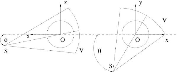
Figure 1.: Scheme of the data acquisition geometry. $(\mathbf{O};x,y,z)$ defines the Carrington heliocentric frame of reference. $S$ is the spacecraft considered. $\phi$ is the latitude, and $\theta$ the longitude of this spacecraft. $V$ is the virtual detector.

We choose to discretize the object in the usual cubic voxels. ${\mathb{x}}$ is a vector of size $N$ containing the values of all voxels. In the same way, we define the vector of data ${\mathb{y}}_{t}$ of size $M$ at time $t$. Since the integration operator is linear, the projection can be described by a matrix ${\mathb{P}}_{t}$. We choose ${\mathb{n}}_{t}$ to be an additive noise:

$${\mathb{y}}_{t}={\mathb{P}}_{t}{\mathb{x}}_{t}+{\mathb{n}}_{t}\text{, }\forall t\in[1,...,T]$$ (1)

${\mathb{P}}_{t}$ is the projection matrix at time $t$ of size $M\times N$ which is defined by the position and the orientation of the spacecraft at this time. Its transpose is the backprojection matrix. Note that a uniform sampling in time is not required. In order to be able to handle large problems with numerous well-resolved data images and a large reconstruction cube, we chose not to store the whole projection matrix. Instead, we perform the projection operation $({\mathb{P}}{\mathb{x}})$ or its transpose each time it is needed at each iteration. Thus, we need a very efficient algorithm. We developed a code written in C which performs the projection operation. It makes use of the geometrical parameters given in the data headers in order to take into account the exact geometry (conicity, position, and orientation of the spacecraft). To keep this operation fast, we implemented the Siddon algorithm Siddon (1985). It allows a fast projection or backprojection in the case of cubic voxels (Cartesian grid). Since we focus on a small region at the poles, we consider that we do not need to use a spherical grid which would require a more time-consuming projection algorithm.

We take into account the fact that the field of view is conical. Despite the fact that the acquisition is very close to the parallel acquisition geometry, it is sufficient to introduce an error of several voxels of size 0.01 solar radius from one side to the other of a three solar radii reconstructed cube.

2.2 Modeling of the Temporal Evolution

With this model, the inverse problem is underdetermined since we have at most three images at one time and we want to reconstruct the object with its temporal evolution. In order to do so, we first redefine our unknowns to separate temporal evolution from spatial structure. We introduce a new set of variables ${\mathb{g}}_{t}$ of size $N$ describing the temporal evolution and require that ${\mathb{x}}$ does not depend on time:

$${\mathb{y}}_{t}={\mathb{P}}_{t}({\mathb{x}}\circ{\mathb{g}}_{t})+{\mathb{n}}_{t}$$ (2)

with $\circ$ being the term-by-term multiplication of vectors. This operator is clearly bilinear. However, this model would increase the number of variables excessively. So, we need to introduce some other kind of a priori into our model. We make the hypothesis that all of the voxels of one polar plume have the same temporal evolution:

$${\mathb{g}}_{t}={\mathb{L}}{\boldsymbol{\theta}}_{t}$$ (3)

The matrix ${\mathb{L}}$ of size $N\times P$ ($P$ being the number of areas) localizes areas where the temporal evolution is identical. Each column of ${\mathb{L}}$ is the support function of one of the plumes. We would like to stress that in our hypothesis, those areas do not move relative to the object. In other words, ${\mathb{L}}$ does not depend on time. Localizing these areas defines ${\mathb{L}}$ and only leaves $P\,T$ variables to estimate. We redefined our problem in a way that limits the number of parameters to estimate but still allows many solutions. Furthermore, the problem is linear in ${\mathb{x}}$ knowing ${\boldsymbol{\theta}}$ and linear in ${\boldsymbol{\theta}}$ knowing ${\mathb{x}}$. It will simplify the inversion of the problem as we shall see later. Note, however that the uniqueness of a solution $({\mathb{x}},{\boldsymbol{\theta}})$ is not guaranteed with bilinearity despite its being guaranteed in the linear case. This example shows that $A$ can be chosen arbitrarily without changing the closeness to the data: ${\mathb{x}}\circ{\mathb{g}}=(A{\mathb{x}})\circ(A^{-1}{\mathb{g}})$, where $A$ is a real constant. Introducing an a priori of closeness to ${\mathbf{1}}$ for ${\boldsymbol{\theta}}$ would allow us to deal with this indeterminacy in principle. But note that this indeterminacy is not critical since the physical quantity of interest is only the product ${\mathb{x}}\circ{\mathb{g}}$. Féron, Duchêne, and Mohammad-Djafari (2005) present a method which solves a bilinear inversion problem in the context of microwave tomography.

We do not deal with the estimation of the areas undergoing evolution, but we assume in this paper that the localization is known. This localization can be achieved using other sources of information, e.g. stereoscopic observations. We expect to be able to locate the areas using some other source of information.

We can regroup the equations of the direct problem. We have two ways to do so, each emphasizing the linearity throughout one set of variables.

$$\begin{array}[]{c}{\mathb{y}}={\mathb{U}}_{\mathb{x}}{\boldsymbol{\theta}}+{\mathb{n}}\\ \left(\begin{array}[]{c}{\mathb{y}}_{1}\\ \vdots\\ {\mathb{y}}_{T}\end{array}\right)=\left(\begin{array}[]{ccc}{\mathb{P}}_{1}{\mathb{X}}{\mathb{L}}&&\mathbf{0}\\ &\ddots&\\ \mathbf{0}&&{\mathb{P}}_{T}{\mathb{X}}{\mathb{L}}\end{array}\right)\par\left(\begin{array}[]{c}{\boldsymbol{\theta}}_{1}\\ \vdots\\ {\boldsymbol{\theta}}_{T}\end{array}\right)+\left(\begin{array}[]{c}{\mathb{n}}_{1}\\ \vdots\\ {\mathb{n}}_{T}\end{array}\right)\par\end{array}$$ (4)

with ${\mathb{X}}=diag({\mathb{x}})$, the diagonal matrix defined by ${\mathb{x}}$. ${\mathb{x}}$ is of size $N$, ${\mathb{y}}$ and ${\mathb{n}}$ are of size $M\,T$, ${\boldsymbol{\theta}}$ is of size $P\,T$ and ${\mathb{U}}_{\mathb{x}}$ is of size $M\,T\times P\,T$.

Similarly,

$$\begin{array}[]{c}{\mathb{y}}={\mathb{V}}_{\boldsymbol{\theta}}{\mathb{x}}+{\mathb{n}}\\ \text{ with }{\mathb{V}}_{\boldsymbol{\theta}}=\left(\begin{array}[]{ccc}{\mathb{P}}_{1}{\mathrm{diag}}({\mathb{L}}{\boldsymbol{\theta}}_{1})&&\mathbf{0}\\ &\ddots&\\ \mathbf{0}&&{\mathb{P}}_{T}{\mathrm{diag}}({\mathb{L}}{\boldsymbol{\theta}}_{T})\end{array}\right)\left(\begin{array}[]{c}{\mathb{I}}_{d}\\ \vdots\\ {\mathb{I}}_{d}\end{array}\right)\end{array}$$ (5)

with ${\mathb{I}}_{d}$ the identity matrix of size $M\times M$. ${\mathb{V}}_{\boldsymbol{\theta}}$ is of size $MT\times N$.

2.3 Inverse Problem

In Bayes’ formalism, solving an inverse problem consists in knowing the a posteriori (the conditional probability density function of the parameters, the data being given). To do so we need to know the likelihood (the conditional probability density function of the data knowing the parameters) and the a priori (the probability density function of the parameters). An appropriate model is a Gaussian, independent, identically distributed (with the same variance) noise ${\mathb{n}}$. The likelihood function is deduced from the noise statistic:

$$f({\mathb{y}}|{\mathb{x}},{\boldsymbol{\theta}},\sigma_{n},\mathcal{M})=K_{1}\exp\left(-\frac{\|{\mathb{y}}-{\mathb{U}}_{\mathb{x}}{\boldsymbol{\theta}}\|^{2}}{2\sigma_{\mathb{n}}^{2}}\right)$$ (6)

$\mathcal{M}=\left[{\mathb{P}},{\mathb{L}}\right]$ describing our model (the projection algorithm and parameters and the choice of the plume position). We assume that the solution is smooth spatially and temporally, so we write the a priori as follows:

$$f({\mathb{x}}|\sigma_{\mathb{x}})=K_{2}\exp\left(-\frac{\|{\mathb{D}}_{r}{\mathb{x}}\|^{2}}{2\sigma_{\mathb{x}}^{2}}\right)\textrm{ and }f({\boldsymbol{\theta}}|\sigma_{\boldsymbol{\theta}})=K_{3}\exp\left(-\frac{\|{\mathb{D}}_{t}{\boldsymbol{\theta}}\|^{2}}{2\sigma_{\boldsymbol{\theta}}^{2}}\right)$$ (7)

${\mathb{D}}_{r}$ and ${\mathb{D}}_{t}$ are discrete differential operators in space and time. Bayes’ theorem gives us the a posteriori law if we assume that the model $\mathcal{M}$ is known as well as the hyperparameters $\mathcal{H}=\left[\sigma_{\mathb{n}},\sigma_{\mathb{x}},\sigma_{\boldsymbol{\theta}}\right]$:

$$f({\mathb{x}},{\boldsymbol{\theta}}|{\mathb{y}},\mathcal{H},\mathcal{M})=\frac{f({\mathb{y}}|{\mathb{x}},{\boldsymbol{\theta}},\sigma_{\mathb{n}},\mathcal{M})f({\mathb{x}}|\sigma_{\mathb{x}})f({\boldsymbol{\theta}}|\sigma_{\boldsymbol{\theta}})}{f({\mathb{y}}|\mathcal{H},\mathcal{M})}$$ (8)

We need to choose an estimator. It allows us to define a unique solution instead of having a whole probability density function. We then choose to define our solution as the maximum a posteriori. which is given by:

$$({\mathb{x}}^{\scriptscriptstyle\text{MAP}},{\boldsymbol{\theta}}^{\scriptscriptstyle\text{MAP}})=\mathop{\mathrm{arg\,max}}_{{\mathb{x}},{\boldsymbol{\theta}}}f({\mathb{y}}|{\mathb{x}},{\boldsymbol{\theta}},\sigma_{\mathb{n}},\mathcal{M})f({\mathb{x}}|\sigma_{\mathb{x}})f({\boldsymbol{\theta}}|\sigma_{\boldsymbol{\theta}})$$ (9)

since $f({\mathb{y}}|\mathcal{M})$ is a constant. Equation (9) can be rewritten as a minimization problem:

$$({\mathb{x}}^{\scriptscriptstyle\text{MAP}},{\boldsymbol{\theta}}^{\scriptscriptstyle\text{MAP}})=\mathop{\mathrm{arg\,min}}_{{\mathb{x}},{\boldsymbol{\theta}}}J({\mathb{x}},{\boldsymbol{\theta}})$$ (10)

with:

$$J({\mathb{x}},{\boldsymbol{\theta}})=-2\sigma_{n}\log f({\mathb{x}},{\boldsymbol{\theta}}|{\mathb{y}},\mathcal{M},\mathcal{H})=\|{\mathb{y}}-{\mathb{U}}_{\mathb{x}}{\boldsymbol{\theta}}\|^{2}+\lambda\|{\mathb{D}}_{r}{\mathb{x}}\|^{2}+\mu\|{\mathb{D}}_{t}{\boldsymbol{\theta}}\|^{2}$$

$\lambda=\frac{\sigma_{n}^{2}}{\sigma_{x}^{2}}$ and $\mu=\frac{\sigma_{n}^{2}}{\sigma_{\alpha}^{2}}$ are user-defined hyperparameters.

The equivalence of Equations (9) and (10) has been proved by Demoment89.

Note that the solution does not have to be very smooth. It mostly depends on the level of noise since noise increases the underdetermination of the problem as it has been shown by the definition of $\lambda$ and $\mu$.

2.4 Criterion Minimization

The two sets of variables ${\mathb{x}}$ and ${\boldsymbol{\theta}}$ are very different in nature. However, thanks to the problem’s bilinearity, one can easily estimate one set while the other is fixed. Consequently we perform an iterative minimization of the criterion, and we alternate minimization of ${\mathb{x}}$ and ${\boldsymbol{\theta}}$. At each step $n$ we perform:

$${\boldsymbol{\theta}}^{n+1}=\mathop{\mathrm{arg\,min}}_{\boldsymbol{\theta}}J({\mathb{x}}^{n},{\boldsymbol{\theta}})\text{ and }{\mathb{x}}^{n+1}=\mathop{\mathrm{arg\,min}}_{\mathb{x}}J({\mathb{x}},{\boldsymbol{\theta}}^{n+1})$$ (11)

The two subproblems are formally identical. However, ${\boldsymbol{\theta}}$ is much smaller than ${\mathb{x}}$. This is of the utmost practical importance since one can directly find the solution on ${\boldsymbol{\theta}}$ by using the pseudo-inverse method. ${\mathb{x}}$ is too big for this method, and we have to use an iterative scheme such as the conjugate-gradient to approximate the minimum. These standard methods are detailed in Appendices A and B.

2.5 Descent Direction Definition and Stop Threshold

We choose to use an approximation of the conjugate-gradient method that is known to converge much more rapidly than the simple gradient method Nocedal and Wright (2000); Polak and Ribière (1969).

$$\begin{array}[]{ccc}{\mathb{d}}^{p+1}&=&{\mathb{d}}^{p}+b^{p}{\bf\nabla}_{{\mathb{x}}}\left.J\right|_{{\mathb{x}}={\mathb{x}}^{p}}\\ b^{p}&=&\frac{\left<{\bf\nabla}_{{\mathb{x}}}\left.J\right|_{{\mathb{x}}={\mathb{x}}^{p}},{\bf\nabla}_{{\mathb{x}}}\left.J\right|_{{\mathb{x}}={\mathb{x}}^{p-1}}\right>}{\|{\bf\nabla}_{{\mathb{x}}}\left.J\right|_{{\mathb{x}}={\mathb{x}}^{p-1}}\|^{2}}\end{array}$$ (12)

Since the minimum is only approximately found, we need to define a threshold which we consider to correspond to an appropriate closeness to the data in order to stop the iterations. Since the solution is the point at which the gradient is zero, we choose this threshold for updating $x$:

$$\text{mean}_{{\mathb{x}}\in[{\mathb{x}}^{p},{\mathb{x}}^{p-1},{\mathb{x}}^{p-2}]}\|{\bf\nabla}_{{\mathb{x}}}J\|^{2}<S_{x}$$ (13)

For the global minimization, the gradient is not computed, so we choose:

$$\text{mean}_{[n,n-1,n-2]}\|({\mathb{x}}_{n},{\boldsymbol{\theta}}_{n})-({\mathb{x}}_{n-1},{\boldsymbol{\theta}}_{n-1})~\|^{2}<S_{G}$$ (14)

Note that this way to stop the iteration allows one to define how close one wants to be to the solution: if the difference between two steps is below this threshold, it is considered negligible. The algorithm can be summarized as shown in Figure 2.

• ${\mathb{x}}=0$ and ${\boldsymbol{\theta}}=1$

• Equation (14) is satisfied

  • Equation (13) is satisfied

    • compute gradient at ${\mathb{x}}_{n}$ with Equation (19)

    • compute descent direction with Equation (12)

    • compute optimum step with Equation (21)

    • update ${\mathb{x}}$ with Equation (22)

  • • compute the matrix ${\mathb{U}}_{{\mathb{x}}^{n}}^{T}{\mathb{U}}_{{\mathb{x}}^{n}}$ and the vector ${\mathb{U}}_{{\mathb{x}}^{n}}^{T}{\mathb{y}}$

    • inverse the matrix ${\mathb{U}}_{{\mathb{x}}^{n}}^{T}{\mathb{U}}_{{\mathb{x}}^{n}}+\mu{\mathb{D}}_{r}^{T}{\mathb{D}}_{r}$

    • compute Equation (18)

Figure 2.: Tomographic Reconstruction with Temporal Evolution Algorithm

3 Method Validation

In order to validate the principle of our method and test its limits, we simulate an object containing some plumes with temporal evolution and try to extract it from the data.

3.1 Simulation Generation Process

We generate an emission cube with randomly-placed, ellipsoidal plumes with a Gaussian shape along each axis:

$$E_{p}=A\exp\left(-\frac{1}{2}\left[\frac{{\mathb{r}}.{\mathb{u}}_{\phi})}{a}\right]^{2}-\frac{1}{2}\left[\frac{{\mathb{r}}.{\mathb{u}}_{\phi+\frac{\pi}{2}}}{b}\right]^{2}\right)$$ (15)

The plumes evolve randomly but smoothly by interpolating over a few randomly generated points. Once the object is generated, we compute a typical set of 60 images equally spaced along 180^∘ using our projector algorithm. A Gaussian random noise is added to the projections with a signal to noise ratio (SNR) of five. The simulation parameters are summarized in Table 1.

Plume	Semimajor	Semiminor	$\phi$	$x_{0}$	$y_{0}$	Intensity
Number	Axis $a$	Axis $b$				$(A)$
1	4.8	4.2	1.2	29	29	329
2	5.6	3.3	1.1	23	33	430
3	5.2	4.8	0.1	40	42	723

Table 1.: Simulation Definition: Plumes Parameters

cube size	cube number	pixel	projection
(solar radii)	of voxels	size (radians)	number of pixels
$1\times 1\times 0.05$	$64\times 64\times 4$	$5\times 10^{-5}\times 5\times 10^{-5}$	$128\times 8$

Table 2.: Simulation Definition: Geometric Parameters

SNR	$\lambda$	$\mu$	$S_{\mathb{x}}$	$S_{G}$
$5$	$2\times 10^{-2}$	$100$	$2\times 10^{-2}$	$1\times 10^{-2}$

Table 3.: Simulation Definition: Other Parameters

3.2 Results Analysis

We now compare our results (Figure 3) with a filtered back-projection (FBP) algorithm. This method is explained by Natterer86 and Kak87.

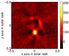
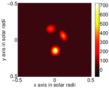
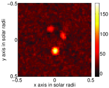
(a) ${\mathb{x}}$ with a FBP algorithm	(b) Simulated ${\mathb{x}}$	(c) ${\mathb{x}}$ with our algorithm
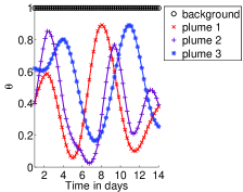
(d) Chosen temporal areas	(e) Simulated ${\boldsymbol{\theta}}$	(f) ${\boldsymbol{\theta}}$ with our algorithm

Figure 3.: Comparison of a standard FBP method (a), the real simulated object (b), and the object reconstructed with our method (c). The object is reconstructed using 60 projections regularly spaced over 180^∘. The areas of homogeneous temporal evolution (e) are the same in the simulation and the reconstruction. We associated one time per projection to define ${\boldsymbol{\theta}}$ in the simulation (e) and our reconstruction (f). The time scale is in days assuming a rotation speed of half a rotation in 14 days. ${\mathb{x}}$ is the spatial distribution of the emission density volume. ${\boldsymbol{\theta}}$ is a gain representing the emission variation over time. Except for the FBP reconstruction, only the product ${\mathb{x}}\circ{\boldsymbol{\theta}}$ has physical dimensions. The spatial scales are given in solar radii and centered on the solar axis of rotation. (a), (b) and (c) are slices of 3D cubes at the same $z=0.1\,R_{\odot}$. Emission densities (arbitrary units) are scaled in the color bars in the right-end side of (a), (b), (c).

By comparing the simulation and the reconstruction in Figure 3, we can see the quality of the temporal evolution estimation. The shape of the intensity curves is well reproduced except for the first plume in the first ten time steps where the intensity is slightly underestimated. This corresponds to a period when plume 1 is hidden behind plume 2. Thus, our algorithm attributes part of the plume 1 intensity to plume 2. Let us note that this kind of ambiguity will not arise in the case of observations from multiple points of view such as STEREO/EUVI observations. The indeterminacy of the problem is due to its bilinearity discussed in Section 2.2. This allows the algorithm to attribute larger values to the ${\boldsymbol{\theta}}$ parameters and to compensate by decreasing the corresponding ${\mathb{x}}$. This is not a drawback of the method since it allows discontinuities between plumes and interplumes. The only physical value of interest is the product ${\mathb{x}}\circ{\mathb{g}}$.

Figure 4 shows the relative intensity of the plumes at different times. One can compare with the reconstruction. One way to quantify the quality of the reconstruction is to compute the distance (quadratic norm of the difference) between the real object and the reconstructed one. Since the FBP reconstruction does not actually correspond to a reconstruction at one time, we evaluate the minimum of the distances at each time. We find it to be $3000$. This is to be compared with a value of $700$ with our algorithm, which is much better.

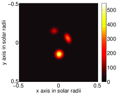
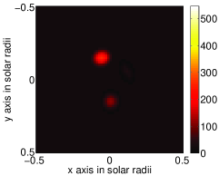
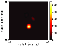
(a) Simulation at $10\Delta T$	(b) Simulation at $30\Delta T$	(c) Simulation at $50\Delta T$
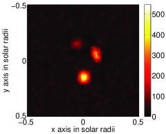
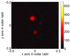
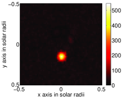
(d) Result at $10\Delta T$	(e) Result at $30\Delta T$	(f) Result at $50\Delta T$

Figure 4.: Comparison of ${\mathb{x}}\circ{\mathb{g}}$ simulated and reconstructed at different times. $\Delta T$ is the time between two data images (5.6 hours). Distances are in solar radii. Values represent the volume emission density. All of this images are slices of 3D cubes at the same $z=0.1R_{\odot}$.

3.3 Choice of Evolution Areas

One can think that the choice of the evolution areas is critical to the good performance of our method. We show in this section that it is not necessarily the case by performing a reconstruction based on simulations with incorrect evolution areas. All parameters and data are exactly the same as in the previous reconstruction. The only difference is in the choice of the areas, i.e. the ${\mathb{L}}$ matrix. These are now defined as shown in Figure 5(a).

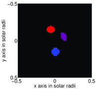
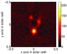
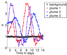
(a) New choice of areas	(b) ${\mathb{x}}$ with our algorithm	(c) ${\boldsymbol{\theta}}$ with our algorithm

Figure 5.: Reconstruction with smaller areas. To be compared with Figure 3. The new areas (a) do not correspond anymore to the ones used to generate the data. (b) is the emission map and (c) the temporal evolution estimated with our algorithm. (b) and (c) are slices of 3D cubes at the same $z=0.1\,R_{\odot}$. Emission densities (arbitrary units) are scaled in the color bars in the right-end side of (b).

Although approximately 50 % of the voxels are not associated with their correct area, we can observe that the algorithm still performs well. The emission map of Figure 5(b) is still better than the emission reconstructed by a FBP method. Plus, the estimation of the temporal evolution in Figure 5(c) corresponds to the true evolution 3(e) even if less precisely than in Figure 3(f).

4 Reconstruction of SOHO/EIT Data

4.1 Data Preprocessing

We now perform reconstruction using SOHO/EIT data. We have to be careful when applying our algorithm to real data. Some problems may arise due to phenomena not taken into account in our model; e.g. cosmic rays, or missing data.

Some of these problems can be handled with simple preprocessing. We consider pixels hit by cosmic rays as missing data. They are detected with a median filter. These pixels and missing blocks are labeled as missing data and the projector and the backprojector do not take them into account (i.e. the corresponding rows in the matrices are removed).

4.2 Results Analysis

In Figures 6 and 7, we present results from 17.1 nm EIT data between 1 and 14 November 1996. This period corresponds to the minimum of solar activity when one can expect to have less temporal evolution. 17.1 nm is the wavelength where the contrast of the plumes is the strongest. Some images are removed resulting in a sequence of 57 irregularly-spaced projections for a total coverage of 191^∘. We assume that we know the position of four evolving plumes as shown on Figure 6(b). For each reconstructed image, we present subareas of the reconstructed cube of size 64$\times$64 centered on the axis of rotation. We assume the rotation speed to be the rigid body Carrington rotation. All of the parameters given in Table 4 and 5 are shared by the different algorithms provided they are required by the method. The computation of this reconstruction on a Intel(R) Pentium(R) 4 CPU 3.00 GHz was 13.5 hours long.

cube size	cube number	pixel	projection
(solar radii)	of voxels	size (radians)	number of pixels
$3\times 3\times 0.15$	$256\times 256\times 8$	$2.55\times 10^{-5}\times 2.55\times 10^{-5}$	$512\times 38$

Table 4.: EIT Data Reconstruction: Geometric Parameters

$\lambda$	$\mu$	$S_{\mathb{x}}$	$S_{G}$
$2\times 10^{-2}$	$1\times 10^{4}$	0.1	0.05

Table 5.: EIT Data Reconstruction : Other Parameters

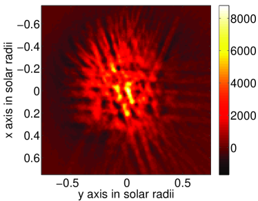
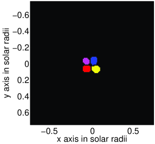
(a) ${\mathb{x}}$ with a FBP algorithm	(b) Chosen temporal areas. Numbered
	clockwise starting from lower-left
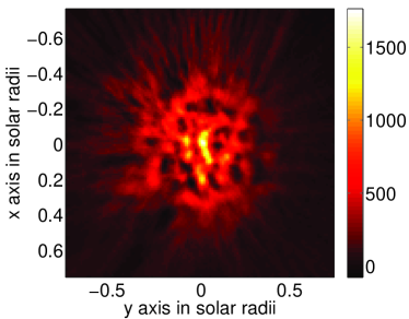
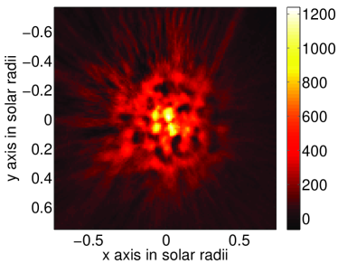
(c) ${\mathb{x}}$ without temporal evolution	(d) ${\mathb{x}}$ with our algorithm

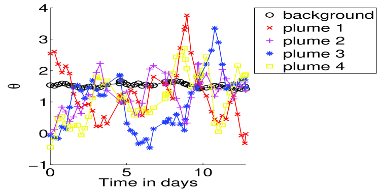
(e) ${\boldsymbol{\theta}}_{t}$ with our algorithm.

Figure 6.: A comparison of FBP (a), a gradient-like algorithm without temporal evolution (c), and our algorithm (d) with real EIT data. ${\mathb{x}}$ is the spatial distribution of the volume emission density integrated over EIT 17.1 nm passband. The chosen areas are shown in (b). ${\boldsymbol{\theta}}$ is a gain representing the emission variation during time (e). The time scale is in days. In the case of our algorithm, only the product ${\mathb{x}}\circ{\boldsymbol{\theta}}$ has physical meaning. The spatial scales are given in solar radii and centered on the solar axis of rotation. (a), (b), (c), and (d) are slices of 3D cubes at the same $z=1.3R_{\odot}$. Emission densities (arbitrary units) are scaled in the color bars in the right-end side of (a), (c), (d).

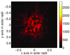
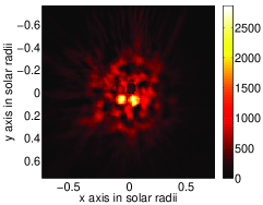
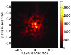
(a) Reconstruction at $t_{25}$	(b) Reconstruction at $t_{35}$	(c) Reconstruction at $t_{45}$
(6 days)	(8.5 days)	(9.8 days)

Figure 7.: Reconstruction of ${\mathb{x}}\circ{\mathb{g}}$ at different times. Distances are in solar radii. Values represent the volume emission density integrated over the EIT 17.1 nm passband. All of these images are slices of 3D cubes at the same $z=1.3\,R_{\odot}.$

Presence of negative values is the indication of a poor behavior of the tomographic algorithm since it does not correspond to actual physical values. We can see in Figure 6 that our reconstruction has many fewer negative values in the ${\mathb{x}}$ map than the FBP reconstruction. In the FBP reconstruction cube, 50% of the voxels have negative values; in the gradient-like reconstruction without temporal evolution 36% of the voxels are negative while in our reconstruction only 25 % are negative. This still seems like a lot but most of these voxels are in the outer part of the reconstructed cube. The average value of the negative voxels is much smaller also. It is -120 for the FBP, -52 for the gradient-like method without temporal evolution, and only -19 for our reconstruction with temporal evolution. However, we notice that the gain coefficients present a few slightly negative values.

In the reconstructions without temporal evolution, plumes three (upper right) and four (lower right) correspond to a unique elongated structure which we choose to divide. Note how our algorithm updated the ${\mathb{x}}$ map reducing the emission values between these two plumes. It shows that what was seen as a unique structure was an artifact resulting from temporal evolution and it tends to validate the usefulness of our model. We note the disappearance of a plume located around (-0.2, -0.15) solar radii on the FBP reconstruction. It shows the utility of gradient-like methods to get rid of artifacts due to the non-uniform distribution of images. Another plume at (0.2, 0.2) solar radii has more intensity in the reconstruction without temporal evolution than with our algorithm. It illustrates how temporal evolution can influence the spatial reconstruction.

5 Discussion

The major feature of our approach is the quality of our reconstruction, which is much improved with respect to FBP reconstruction, as demonstrated by the smaller number of negative values and the increased closeness to the data. Let us now discuss the various assumptions that have been made through the different steps of the method.

The strongest assumption we made, in order to estimate the temporal evolution of polar plumes, is the knowledge of the plume position. Here, we choose to define the plumes as being the brightest points in a reconstruction without temporal evolution. The choice is not based on any kind of automatic threshold. The areas are entirely hand-chosen by looking at a reconstruction. It is possible that these areas do not correspond to the actual physical plumes, they could correspond to areas presenting increased emission during half a rotation. Note that this is biased in favor of plumes closer to the axis of rotation since, along one slice of the reconstructed cartesian cube, their altitude is lower and thus, their intensity is higher. In order to have constant altitude maps one would have to carry out the computation on a spherical grid or to interpolate afterwards onto such a grid. For this reconstruction example we are aware that we did not locate all of the plumes but only tried to find a few. It would be interesting to try to locate the plumes using other data or with a method estimating their positions and shapes.

The method involves hyperparameters which we choose to set manually. There are methods to estimate hyperparameters automatically such as the L-curve method, the cross-validation method Golub, Heath, and Wahba (1979) or the full-bayesian method Higdon et al. (1997); Champagnat, Goussard, and Idier (1996). We performed reconstructions using different hyperparameter values. We then looked at the reconstruction to see if the smoothness seemed exaggerated or if the noise were amplified in the results. This allowed us to reduce the computational cost and does not really put the validity of the method into question.

One possible issue with this algorithm is the non-convexity of our criterion. This can lead to the convergence to a local minimum that does not correspond to the desired solution defined as the global minimum of the criterion. One way to test this would be to change the initialization many times.

We chose the speed of rotation of the poles to be the Carrington rotation speed. But the speed of the polar structures has not been measured precisely to our knowledge and could affect drastically the reconstruction. This is an issue shared by all tomographic reconstructions of the Sun.

In the current approach, we need to choose on our own the position of the time-evolving areas which are assumed to be plumes. This is done by assuming that more intense areas of a reconstruction without temporal evolution correspond to plume positions. A more rigorous way would be to try to use other sources of information to try to localize the plumes. Another, self-consistent way, would be to develop a method that jointly estimates the position of the plumes in addition to the emission (${\mathb{x}}$) and the time evolution (${\boldsymbol{\theta}}$). We could try to use the results of Yu and Fessler (2002) who propose an original approach in order to reconstruct a piece-wise homogeneous object while preserving edges. The minimization is alternated between an intensity map and boundary curves. The estimation of the boundary curves is made using level sets technics (Yu and Fessler (2002) and references therein). It would also be possible to use a Gaussian mixture model Snoussi and Mohammad-Djafari (2007).

6 Conclusion

We have described a method that takes into account the temporal evolution of polar plumes for tomographic reconstruction near the solar poles. A simple reconstruction based on simulations demonstrates the feasibility of the method and its efficiency in estimating the temporal evolution assuming that parameters such as plume position or rotation speed are known. Finally we show that it is possible to estimate the temporal evolution of the polar plumes with real data.

In this study we limited ourselves to reconstruction of images at 17.1 nm but one can perform reconstructions at 19.5 nm and 28.4 nm as well. It would allow us to estimate the temperatures of the electrons as in Frazin, Kamalabadi, and Weber (2005) or Barbey et al.(2006).

Acknowledgements

Nicolas Barbey acknowledges the support of the Centre National
d’Études Spatiales and the Collecte Localisation Satellites. The authors thank the referee for their useful suggestions for the article.

Appendix A Pseudo-Inverse Minimization

We want to minimize:

$$J=\|{\mathb{y}}-{\mathb{U}}_{{\mathb{x}}^{n}}{\boldsymbol{\theta}}\|^{2}+\lambda\|{\mathb{D}}_{r}{\mathb{x}}^{n}\|^{2}+\mu\|{\mathb{D}}_{t}{\boldsymbol{\theta}}\|^{2}$$ (16)

The second term does not depend on ${\boldsymbol{\theta}}$. Due to the strict convexity of the criterion, the solution is a zero of the gradient. Since the criterion is quadratic, one can explicitly determine the solution:

$$\left.{\bf\nabla}_{{\boldsymbol{\theta}}}J\right|_{{\boldsymbol{\theta}}={\boldsymbol{\theta}}^{n+1}}=2{\mathb{U}}_{{\mathb{x}}^{n}}^{T}\left({\mathb{U}}_{{\mathb{x}}^{n}}{\boldsymbol{\theta}}^{n+1}-{\mathb{y}}\right)+2\mu{\mathb{D}}_{t}^{T}{\mathb{D}}_{t}{\boldsymbol{\theta}}^{n+1}=\mathbf{0}$$ (17)

from which we conclude:

$${\boldsymbol{\theta}}^{n+1}=\left[{\mathb{U}}_{{\mathb{x}}^{n}}^{T}{\mathb{U}}_{{\mathb{x}}^{n}}+\mu{\mathb{D}}_{t}^{T}{\mathb{D}}_{t}\right]^{-1}{\mathb{U}}_{{\mathb{x}}^{n}}^{T}{\mathb{y}}$$ (18)

Appendix B Gradient-like Method

In this method we try to find an approximation of the minimum by decreasing the criterion iteratively. The problem is divided in two subproblems: searching for the direction and searching for the step of the descent. In gradient-like methods, the convergence is generally guaranteed ultimately to a local minimum. But since the criterion is convex, the minimum is global. To iterate, we start at an arbitrary point $({\mathb{x}}^{0})$ and go along a direction related to the gradient. The gradient at the $p^{th}$ step is:

$$\left.{\bf\nabla}_{{\mathb{x}}}J\right|_{{\mathb{x}}={\mathb{x}}^{p}}=2{\mathb{V}}_{{\boldsymbol{\theta}}^{n+1}}^{T}\left({\mathb{V}}_{{\boldsymbol{\theta}}^{n+1}}{\mathb{x}}^{p}-{\mathb{y}}\right)+2\lambda{\mathb{D}}_{r}^{T}{\mathb{D}}_{r}{\mathb{x}}^{p}$$ (19)

Once the direction is chosen, searching for the optimum step is a linear minimization problem of one variable:

$$a_{\scriptscriptstyle\text{OPT}}^{p+1}=\mathop{\mathrm{arg\,min}}_{a}J({\mathb{x}}^{p}+a{\mathb{d}}^{p+1})$$ (20)

which is solved by:

$$a_{\scriptscriptstyle\text{OPT}}^{p+1}=-\frac{1}{2}\frac{{\mathb{d}}^{p+1}\left.{\bf\nabla}_{{\mathb{x}}}J\right|_{{\mathb{x}}={\mathb{x}}^{p}}}{\|{\mathb{V}}_{{\boldsymbol{\theta}}^{n+1}}{\mathb{d}}^{p+1}\|^{2}+\lambda\|{\mathb{D}}_{r}{\mathb{d}}^{p+1}\|^{2}}$$ (21)

We can write the iteration:

$${\mathb{x}}^{p+1}={\mathb{x}}^{p}+a_{\scriptscriptstyle\text{OPT}}^{p+1}{\mathb{d}}^{p+1}$$ (22)

References

- Barbey et al. (2006) Barbey, N., Auchére, F., Rodet, T., Bocchialini, K., Vial, J.C.: 2006, Rotational Tomography of the Solar Corona-Calculation of the Electron Density and Temperature. In: Lacoste, H. (ed.) SOHO 17 - 10 Years of SOHO and Beyond. ESA Special Publications. ESA Publications Division, Noordwijk, 66 – 68.
- Barbey et al. (2007) Barbey, N., Auchère, F., Rodet, T., Vial, .J.C.: 2007, Reconstruction Tomographique de Séquences d’Images 3D - Application aux Données SOHO/STEREO. In: Actes de GRETSI 2007., 709 – 712.
- Champagnat, Goussard, and Idier (1996) Champagnat, F., Goussard, Y., Idier, J.: 1996, Unsupervised deconvolution of sparse spike trains using stochastic approximation. IEEE Transactions on Signal Processing 44(12), 2988 – 2998.
- DeForest, Lamy, and Llebaria (2001) DeForest, C.E., Lamy, P.L., Llebaria, A.: 2001, Solar Polar Plume Lifetime and Coronal Hole Expansion: Determination from Long-Term Observations. Astrophys. J. 560, 490 – 498.
- Demoment (1989) Demoment, G.: 1989, Image reconstruction and restoration: Overview of common estimation structure and problems. IEEE Transactions on Acoustics, Speech and Signal Processing 37(12), 2024 – 2036.
- Féron, Duchêne, and Mohammad-Djafari (2005) Féron, O., Duchêne, B., Mohammad-Djafari, A.: 2005, Microwave imaging of inhomogeneous objects made of a finite number of dielectric and conductive materials from experimental data. Inverse Problems 21(6), S95 – S115.
- Frazin (2000) Frazin, R.A.: 2000, Tomography of the Solar Corona. I. A Robust, Regularized, Positive Estimation Method. Astrophys. J. 530, 1026 – 1035.
- Frazin et al. (2005) Frazin, R.A., Butala, M.D., Kemball, A., Kamalabadi, F.: 2005, Time-dependent Reconstruction of Nonstationary Objects with Tomographic or Interferometric Measurements. ApJ 635(2), L197 – L200.
- Frazin and Janzen (2002) Frazin, R.A., Janzen, P.: 2002, Tomography of the Solar Corona. II. Robust, Regularized, Positive Estimation of the Three-dimensional Electron Density Distribution from LASCO-C2 Polarized White-Light Images. Astrophys. J. 570, 408 – 422.
- Frazin and Kamalabadi (2005) Frazin, R.A., Kamalabadi, F.: 2005, Rotational Tomography For 3D Reconstruction Of The White-Light And Euv Corona In The Post-SOHO Era. Sol. Phys. 228, 219 – 237.
- Frazin, Kamalabadi, and Weber (2005) Frazin, R.A., Kamalabadi, F., Weber, M.A.: 2005, On the Combination of Differential Emission Measure Analysis and Rotational Tomography for Three-dimensional Solar EUV Imaging. ApJ 628, 1070 – 1080.
- Gabriel et al. (2005) Gabriel, A.H., Abbo, L., Bely-Dubau, F., Llebaria, A., Antonucci, E.: 2005, Solar Wind Outflow in Polar Plumes from 1.05 to 2.4 . Astrophys. J. 635, L185 – L188.
- Golub, Heath, and Wahba (1979) Golub, G.H., Heath, M., Wahba, G.: 1979, Generalized cross-validation as a method for choosing a good ridge parameter. Technometrics 21(2), 215 – 223.
- Grass et al. (2003) Grass, M., Manzke, R., Nielsen, T., KoKen, P., Proksa, R., Natanzon, M., Shechter, G.: 2003, Helical cardiac cone beam reconstruction using retrospective ECG gating. Phys. Med. Biol. 48, 3069 – 3083.
- Higdon et al. (1997) Higdon, D.M., Bowsher, J.E., Johnson, V.E., Turkington, T.G., Gilland, D.R., Jaszczak, R.J.: 1997, Fully Bayesian estimation of Gibbs hyperparameters for emission computed tomography data. IEEE Transactions on Medical Imaging 16(5), 516 – 526.
- Kachelriess, Ulzheimer, and Kalender (2000) Kachelriess, M., Ulzheimer, S., Kalender, W.: 2000, ECG-correlated imaging of the heart with subsecond multislice spiral CT. IEEE Transactions on Medical Imaging 19(9), 888 – 901.
- Kak and Slaney (1987) Kak, A.C., Slaney, M.: 1987, Principles of computerized tomographic imaging. IEEE Press, New York.
- Llebaria, Saez, and Lamy (2002) Llebaria, A., Saez, F., Lamy, P.: 2002, The fractal nature of the polar plumes. In: Wilson, A. (ed.) ESA SP-508: From Solar Min to Max: Half a Solar Cycle with SOHO., 391 – 394.
- Natterer (1986) Natterer, F.: 1986, The Mathematics of Computerized Tomography. John Wiley.
- Nocedal and Wright (2000) Nocedal, J., Wright, S.J.: 2000, Numerical optimization. Series in Operations Research. Springer Verlag, New York.
- Polak and Ribière (1969) Polak, E., Ribière, G.: 1969, Note sur la convergence de méthodes de directions conjuguées. Rev. Française d’Informatique Rech. Opérationnelle 16, 35 – 43.
- Ritchie et al. (1996) Ritchie, C.J., Crawford, C.R., Godwin, J.D., King, K.F., Kim, Y.: 1996, Correction of computed tomography motion artifacts using pixel-specific backprojection. IEEE Med. Imag. 15(3), 333 – 342.
- Roux et al. (2004) Roux, S., Debat, L., Koenig, A., Grangeat, P.: 2004, Exact reconstruction in 2d dynamic CT: compensation of time-dependent affine deformations. Phys. Med. Biol. 49(11), 2169 – 2182.
- Siddon (1985) Siddon, R.L.: 1985, Fast calculation of the exact radiological path for a three-dimensional CT array. Medical Physics 12, 252 – 255.
- Snoussi and Mohammad-Djafari (2007) Snoussi, H., Mohammad-Djafari, A.: 2007, Estimation of structured Gaussian mixtures: the inverse EM algorithm. IEEE Trans. on Signal Processing 55(7), 3185 – 3191.
- Teriaca et al. (2003) Teriaca, L., Poletto, G., Romoli, M., Biesecker, D.A.: 2003, The Nascent Solar Wind: Origin and Acceleration. Astrophys. J. 588, 566 – 577.
- Wiegelmann and Inhester (2003) Wiegelmann, T., Inhester, B.: 2003, Magnetic modeling and tomography: First steps towards a consistent reconstruction of the solar corona. Solar Physics 214, 287 – 312.
- Yu and Fessler (2002) Yu, D., Fessler, J.: 2002, Edge-preserving tomographic reconstruction with nonlocal regularization. IEEE Med. Imag. 21, 159 – 173.