The transport of cosmic rays in self-excited magnetic turbulence

Abstract

The process of diffusive shock acceleration relies on the efficacy with which hydromagnetic waves can scatter charged particles in the precursor of a shock. The growth of self-generated waves is driven by both resonant and non-resonant processes. We perform high-resolution magnetohydrodynamic simulations of the non-resonant cosmic-ray driven instability, in which the unstable waves are excited beyond the linear regime. In a snapshot of the resultant field, particle transport simulations are carried out. The use of a static snapshot of the field is reasonable given that the Larmor period for particles is typically very short relative to the instability growth time. The diffusion rate is found to be close to, or below, the Bohm limit for a range of energies. This provides the first explicit demonstration that self-excited turbulence reduces the diffusion coefficient and has important implications for cosmic ray transport and acceleration in supernova remnants.

1 Introduction

Supernova remnants (SNR) have long been identified as possible locations for the production and acceleration of galactic cosmic rays. The diffusive shock acceleration mechanism provides a natural explanation for the observed power-law spectrum for these cosmic rays. Acceleration to high energies relies on confinement of relativistic particles to the accelerating region close to the shock. Pitch-angle scattering from self-produced hydromagnetic waves can provide a suitable mechanism, but a detailed analysis demonstrates that the spectrum still falls short of the cosmic ray knee at $\approx 10^{15}$ eV (Lagage & Cesarsky, 1983). However, theory dictates that the maximum energy of the cosmic rays is determined by the diffusion coefficient, which is assumed to scale with the strength of the ambient magnetic field. Therefore, in the quasilinear framework, amplification of the apparent ambient magnetic field in the vicinity of the shock facilitates acceleration to higher energies.

To within an order of magnitude the timescale for the diffusive shock acceleration of a particle is $t_{\rm acc}\approx{\kappa}/{v_{\rm sh}^{2}}$ where $\kappa\equiv\lim_{t\to\infty}\langle\Delta^{2}r\rangle/2t$ is the asymptotic spatial diffusion coefficient where $\Delta r$ is the spatial displacement over time interval $t$. The conventional approximation for transport of particles of speed $v$ via scattering is Bohm diffusion which assumes a single scattering event occurs during each Larmor time.

In the region upstream of a shock, the scattering of particles is due to resonant collisions with slowly moving magnetic irregularities which, in turn, are amplified by such interactions themselves. These turbulent irregularities, until recently, have been assumed to saturate at levels $\delta B\lesssim B_{0}$ (McKenzie & Völk, 1982). With such turbulence, Bohm diffusion can be taken as a lower limit for the diffusion coefficient, $\kappa\,\raisebox{-1.72218pt}{$\stackrel{{\scriptstyle>}}{{\scriptstyle\sim}}$}\,\kappa_{\rm Bohm}$. In highly turbulent fields, however, numerical investigations suggest that particle transport properties may differ significantly from this approximation (Casse, Lemoine & Pelletier, 2002).

Bell & Lucek (2001) proposed a process of resonant amplification of the magnetic field driven by the pressure gradient of cosmic rays, allowing rapid transfer of energy into the Alfvén waves. Amplification factors of $\delta B/B_{0}\sim 1000$ were estimated from the linear theory, although this value is possibly excessive as the analysis most likely does not hold beyond $\delta B/B_{0}\sim 1$. Nevertheless, a more detailed non-linear analysis does suggest acceleration up to $E_{\rm max}\sim 10^{16}{\rm eV}$. In particular, under expansion into a stellar wind, it may even be possible to achieve proton energies of the order $E_{\rm max}\sim 10^{17}$eV via this process.

Moving beyond this result, Bell (2004) identified a non-resonant instability driven by streaming, positively charged cosmic rays that operates on length scales much shorter than the Larmor radius $r_{\rm g}\equiv p/eB_{0}$ of the driving particles (where $p$ is the particle momentum, $e$ is the electronic charge, and $B_{0}$ is the mean magnetic field magnitude). Crucially, under typical conditions in the precursor of a high Alfvén-Mach-number supernova remnant shock, the growth rate for this non-resonant instability can be several orders of magnitude greater than that of its resonant counterpart. Indeed, numerical magnetohydrodynamic simulations carried out in the same work confirmed that field amplification by a factor of an order of magnitude is possible.

Only recently have analytical approaches to particle transport achieved results consistent with numerical approaches. In the case of interplanetary shocks it has been shown that using detailed models of particle transport in turbulent environments sub-Bohm diffusion can be achieved (see Zank et al. (2006) and references therein).

In this paper we investigate, using high resolution MHD simulations, the non-resonant Bell-type instability and its non-linear evolution. We also determine the effective transport properties in the amplified field and compare them with the standard Bohm diffusion description.

The structure of the paper is as follows. In Section 2, we recall the linear MHD analysis of the dispersion relation relevant to the numerical simulations performed. In Section 3 we describe the numerical method used to investigate the non-resonant instability and discuss some properties of the field produced. In Section 4, we describe the techniques used to integrate equations of motion in the snapshot field obtained from the simulations. We discuss the transport properties of both field lines and test particles. Finally, in Section 5, we present our conclusions.

2 The non-resonant instability

Following Bell (2004), we determine the dispersion relation for waves in the precursor of a quasi-parallel non-relativistic shock, where the energy density of the cosmic rays is comparable to the ram pressure of the shock ($\sim 10\%$). The usual assumptions made in the linear analysis of MHD waves propagating in a plasma are that the plasma is quasi-neutral, i.e. is charge neutral on aggregate. Therefore, assuming a plasma consisting entirely of protons and electrons in the presence of a pure proton cosmic ray component, the thermal plasma has a charge excess of electrons. In the reference frame in which the upstream protons are at rest, the cosmic rays are seen to stream with a group velocity approximately equal to the shock velocity, $\langle v\rangle\approx{v}_{\rm sh}$. A charge flux is induced in thermal plasma to neutralise this current. In the case of a mean field $\mathbf{B}_{\|}$ parallel to the shock normal, this return current has a mean (unperturbed) value given by $\mathbf{j}_{\|}=n_{cr}e\mathbf{v}_{\rm sh}$ where $n_{cr}$ is the number density of cosmic rays and $e$ is the electronic charge. The momentum equation is given in the MHD approximation by

$$\rho\frac{{\rm d}{\bf u}}{{\rm d}t}=-\nabla P+{\bf j}_{\rm th}\times{\bf B},$$ (1)

where ${\bf j}_{\rm th}$, the current density carried by the thermal plasma, is determined by Ampère’s law,

$$\nabla\times{\bf B}=\mu_{0}\sum_{s}n_{s}q_{s}{\bf v}_{s}=\mu_{0}({\bf j}_{\rm th}+{\bf j}_{\rm cr}),$$ (2)

where $s$ is an index used to sum over the charged species and $\mu_{0}$ is the plasma permeability. The zeroth order cosmic-ray current density is parallel to the mean magnetic field, which is chosen to lie along the z-axis. All first order perturbations are taken to lie perpendicular to the zeroth order components such that the magnetic field and cosmic-ray current density can be expressed as $\mathbf{B}=\mathbf{B}_{\|}+\mathbf{B}_{\perp}$, $\mathbf{j}_{\rm cr}=\mathbf{j}_{\|}+\mathbf{j}_{\perp}$ respectively. Making use of the induction equation

$$\frac{\partial{\bf B}}{\partial t}=\nabla\times({\bf u\times B})$$ (3)

we look for plane-wave solutions to the linearised system with $\mathbf{k}$ also parallel to the mean field. All first order quantities $\mathbf{B}_{\perp}$, $\mathbf{j}_{\perp}$, $\mathbf{u}_{\perp}$ and $\mathbf{E}_{\perp}=-\mathbf{u}_{\perp}\times\mathbf{B}_{\|}$, take the circularly polarised form $A_{x}\pm iA_{y}=A_{0}\exp[i(kz-\omega t)]$. For the purposes of analysis, the plasma is taken to be initially at rest.

Using a kinetic description, it was shown by Reville et al. (2007) that for modes with wavenumbers $kr_{\rm g1}\gg 1$, where $r_{\rm g1}\equiv p_{1}/e|B_{\|}|$ is the Larmor radius of the cosmic rays of minimum momentum $p_{1}$, kinetic effects can be neglected i.e. both thermal effects and perturbations to the mean cosmic-ray flux are negligible. Splitting the perpendicular magnetic field perturbation into its cartesian components in the x-y plane the relation

$$\left(\begin{array}[]{cc}\omega^{2}-v_{\rm a}^{2}k^{2}&iB_{\|}j_{\|}k/\rho\\ -iB_{\|}j_{\|}k/\rho&\omega^{2}-v_{\rm a}^{2}k^{2}\end{array}\right)\left(\begin{array}[]{c}B_{x}\\ B_{y}\end{array}\right)=0$$ (8)

is obtained where $v_{\rm a}=B_{\|}/\sqrt{\mu_{0}\rho}$ is the Alfvén speed in the unperturbed field. This system permits several waves, whose dispersion relation takes the form

$$\omega^{2}=k^{2}v_{\rm a}^{2}\pm\zeta v_{\rm sh}^{2}\frac{k}{r_{\rm g1}}$$ (9)

similarly to equation (15) from Bell (2004) where the dimensionless driving parameter $\zeta$ is given by

$$\zeta=\mu_{0}\frac{j_{\|}}{B_{\|}}\frac{v_{\rm a}^{2}}{v_{\rm sh}^{2}}r_{\rm g1}.$$ (10)

It follows that, for strongly driven modes such that $\zeta v_{\rm sh}^{2}/v_{\rm a}^{2}\gg 1$, there exist aperiodic waves (Re $\omega=0$), over the range $1<kr_{\rm g1}<\zeta v_{\rm sh}^{2}/v_{\rm a}^{2}$. From equation (9) it is straight forward to show that the fastest growing mode occurs at

$$k_{\rm max}=\frac{\mu_{0}}{2}\frac{j_{\|}}{B_{\|}}$$ (11)

with growth rate

$$\gamma_{\rm max}=v_{\rm a}k_{\rm max}.$$ (12)

The dispersion relation for arbitrary orientations of $\mathbf{k}$, $\mathbf{j}_{\rm cr}$, and $\mathbf{B}_{0}$ has been determined by Bell (2005) demonstrating that unstable modes exist for all orientations provided $\mathbf{k}\cdot\mathbf{B}_{0}\neq 0$. Melrose (2005) has compared the resonant and non-resonant instabilities for arbitrary angle of propagation and shown that the latter occur with elliptically polarised modes. This emphasises the need for high resolution simulations in three dimensions.

3 Instability Driven Turbulent Field Generation

Our simulation box represents a region in the restframe of the upstream magnetised fluid (shock precursor). We assume a thin box such that both the pressure and density can be taken to be initially constant, and the cosmic rays can be considered unmagnetised (i.e. they travel through the box with straight trajectories).

\psfrag{pp1}[Bl][Bl][1.0][+0]{$t$}\psfrag{pp2}[Bl][Bl][1.0][+0]{$B^{\rm rms}_{\|}$}\psfrag{pp3}[Bl][Bl][1.0][-0]{$B^{\rm rms}_{\perp}$}\includegraphics[width=203.80193pt]{./growth.eps}

Figure 1: The root-mean-square value of the perpendicular (solid) and parallel (dashed) components of the magnetic field. The field is initially damped as the initial energy input goes into kinetic energy, setting the inertial plasma into motion. Once the fluid is in motion the perturbations grow according to the linear analysis as $\exp(\gamma_{\rm max}t)$.

Following Bell (2004) we take typical interstellar values for the upstream quantities $B_{\|}=30{\rm nT}$, nucleon density $n_{0}=1\times 10^{-6}{\rm m}^{-3}$, corresponding to an Alfvén speed $v_{\rm a}=6.6\times 10^{3}{\rm ms}^{-1}$. Furthermore assuming $10\%$ energy transfer to cosmic rays and shock speed $v_{s}/c=1/30$, with $\ln(p_{2}/mc)=14$, where $p_{2}$ is the upper cut-off of the cosmic-ray energy spectrum, we obtain $\zeta=4.8\times 10^{-4}$ and $\zeta v_{s}^{2}=1100v_{\rm a}^{2}$.

In the quasilinear theory of diffusive shock acceleration, the minimum momentum of the cosmic-ray distribution is expected to increase with distance upstream, since lower energy cosmic rays are confined closer to the shock (Eichler, 1979; Blasi, 2002). Assuming Bohm diffusion the minimum cosmic ray momentum at a given distance $z$ upstream of the shock is $p_{1}\approx 3v_{\rm sh}eBz/c$. In order for the non-resonant mode to leave the regime of linear growth before being overtaken by the shock front, i.e., before being advected over a distance of roughly $cr_{\rm g1}/{\rm v}_{\rm sh}$, we take $p_{1}c=1$ PeV (although this is not a lower limit). This gives corresponding physical scales $k^{-1}_{\rm max}=2\times 10^{13}\,{\rm m}$, $\gamma^{-1}_{\rm max}=98\,{\rm yr}$, and $r_{\rm g1}=1.1\times 10^{16}\,{\rm m}$.

3.1 Turbulent seed field

The non-resonant instability develops in a field containing a level of seed turbulence. In the simulations that follow the magnetic field is initialised according to the following prescription

$$\mathbf{B}(x,y,z)=\mathbf{B}_{0}+\mathbf{\delta B}(x,y,z),$$ (13)

where ${\bf\delta B}$ is a small isotropic turbulent field component ($\delta B/B_{0}\ll 1$). The turbulent component is constructed similarly to Giacalone & Jokipii (1994), by choosing $N$ plane-wave modes with random phases, orientations, and polarization states given by

$$\delta{\bf B}({\bf r})=2\sum_{n=1}^{N}A_{n}e^{i({\mathbf{k}}_{n}\cdot\mathbf{r}+\psi_{n})}\hat{\xi}_{n},$$ (14)

where $\mathbf{k}_{n}\equiv k_{n}\hat{\mathbf{e}}_{n}^{1}$. For each mode $n$, $A_{n}$, $\psi_{n}$, $k_{n}$, and $\hat{\mathbf{e}}_{n}^{1}$ are the amplitude, phase, wave-number, and propagation direction respectively. Additionally, the polarization vector $\hat{\xi}_{n}$ is given by

$$\hat{\xi}_{n}\equiv\cos(\alpha_{n})\hat{\mathbf{e}}_{n}^{2}+i\sin(\alpha_{n})\hat{\mathbf{e}}_{n}^{3}$$ (15)

where $\alpha_{n}$ is the polarization angle. The three vectors ($\hat{\mathbf{e}}_{n}^{1}$, $\hat{\mathbf{e}}_{n}^{2}$, $\hat{\mathbf{e}}_{n}^{3}$) form an orthonormal basis for the plane waves such that, for a continuous representation, the field is guaranteed to be solenoidal by the condition $\bf{k}_{n}\cdot\mathbf{\xi}_{n}=0$. However, when the field is projected onto a mesh of uniform spacing $h$ the solenoidal condition on a central-differenced grid is given by O’Sullivan & Downes (2007),

$$\hat{\bf\xi}_{n}\cdot\sin({\bf k}_{n}h)=0.$$ (16)

The amplitude of each mode for a given variance $\sigma^{2}$ is

$$A_{n}^{2}=\sigma^{2}G_{n}\left[\sum_{n=1}^{N}G_{n}\right]^{-1},$$

with

$$G_{n}=\frac{\Delta V_{n}}{1+(k_{n}L_{c})^{\Gamma}}\;\;.$$ (17)

Here $\Gamma$ is the spectral index of the turbulence, and the normalisation factor for three-dimensional turbulence is $\Delta V_{n}=4\pi k_{n}^{2}\Delta k_{n}$. $L_{c}$ is the correlation length of the magnetic field, which in this case we take to be the largest wavelength in the system.

In order to generate the turbulent field component 4 random numbers are required for each mode: two to specify the orientation of the wave-vector $\hat{\mathbf{e}}_{n}^{1}$, and one each for the phase and polarization angles $\psi_{n}$ and $\alpha_{n}$ respectively.

Since the turbulent field will be represented on a periodic mesh, each mode must have an integral number of wavelengths in each coordinate direction. Explicitly, assuming a cubic grid of dimension $L$ with $N$ mesh points in each coordinate direction, $\mathbf{k}=2\pi/L(n_{x},n_{y},n_{z})$ where $n_{x}=0..N/2$ etc. (The factor 2 is necessitated by the hermiticity of $\mathbf{\delta B}$ requiring both negative and positive $k$ modes be allowed.) This geometrical constraint also means that at small $k$, the density of unique modes is low and available $\mathbf{k}$ vectors will have a strong preferential bias along the grid axes. Since isotropic and homogeneous turbulence is only achieved in the limit of $N\to\infty$ (Batchelor, 1982), we do not include modes from the low-$k$ range where this bias is greatest. Additionally, we attenuate the dynamic range at high-$k$ by requiring the shortest scale fluctuations are well resolved over 10 cells (rather than 2 as minimally required above).

3.2 Numerical Scheme

We describe the numerical scheme used to perform the simulations of the non-resonant Bell-type instability. The simulations are performed with considerably higher resolution than those performed previously by Bell (2004). The cosmic-ray current is taken to be uniform along the $z$-axis and constant in time. Kinetic effects are again neglected such that ${\bf j}_{\perp}=0$. For clarity from this point onwards, terms involving magnetic field $\mathbf{B}$ are assumed to have absorbed a factor $1/\sqrt{\mu_{0}}$, and terms involving charge current density $\mathbf{j}$ are assumed to have absorbed a factor $\sqrt{\mu_{0}}$. The MHD equations including cosmic ray current may be written in the form

$$\frac{\partial{\bf U}}{\partial t}+\nabla\cdot{\bf V}={\bf S},$$ (18)

where

$${\bf U}=(\rho,\rho{\bf u},{\bf B},E)^{T}$$ (19)

and

$${\bf V}=\left(\begin{array}[]{c}\rho{\bf u}\\ \rho{\bf uu}+{\bf\mathbb{I}}p^{*}-{\bf BB}\\ {\bf uB-Bu}\\ (E+p^{*}){\bf u}-{\bf(u\cdot B)B}\end{array}\right),$$ (20)

with $p^{*}=p+B^{2}/2$, the total pressure. The source terms are given by

$${\bf S}=\left(\begin{array}[]{c}0\\ -j_{\|}{\bf\hat{z}}\times{\bf B}\\ 0\\ -{\bf u}\cdot(j_{\|}{\bf\hat{z}}\times{\bf B})\end{array}\right).$$ (21)

We have constructed a finite volume Godunov code in three dimensions, MENDOZA, which follows the method described in Falle et al. (1998). The equations are split into three one-dimensional problems to find the fluxes on the surface of each cell. The fluxes are determined at each cell interface from the solution to the linearised Riemann problem, and the field is updated with second-order accuracy in both time and space. The source terms are then added as explicit volume-averaged quantities. We have investigated a variety of divergence cleaning methods, but found the generalised Lagrangian multiplier (GLM) method of Dedner et al. (2002) to be most effective. Divergence errors are naturally produced in multidimensional simulations, due to the fact that the one-dimensional problem is solved for each direction and the fluxes simply added together. While the GLM method does not identically conserve $\nabla\cdot{\bf B}=0$, it has the unique property of rapidly damping any divergence introduced, while advecting them away from the problem areas at the fastest admissible speed. For the study of magnetic instabilities, particularly in the presence of strong pressure gradients, we find this method to have many advantages over correction schemes. For a comparison of many different divergence cleaning methods see, for example, Tóth (2000).

Using simulation units, the model is then initialised with

$P=\rho=1$ ,

$j_{\|}=4\pi/5$ ,

$B_{\|}=1$ ,

$\mathbf{u}=0$ .

Equations (10) to (12) then yield

$v_{\rm a}=1$ ,	$v_{\rm sh}=1520$ ,	$k_{\rm max}=2\pi/5$ ,
$\gamma_{\rm max}=2\pi/5$ ,	$r_{\rm g1}=1375/\pi$ .

As is common practice in the literature, the turbulent field spectrum is represented by a superposition of plane wave modes, one selected in a random direction from each of a number of uniform intervals of $\log k$ over a finite range. As commented in Section 3.1 however, since a discrete mesh is being used to represent a periodic field, viable $k$-vectors are finite in number and may be clustered or multiply degenerate in $k$. Therefore, for a given grid resolution, requiring that each interval contains at least one viable $k$-vector determines the total number of modes used to construct the turbulent field representation and the cutoffs in the power spectrum. In this work, a $512^{3}$ grid is used with modes in the range $40\leq kL\leq 550$. With these parameters the number of modes we obtain is $N=151$. While this dynamic range ($\sim 14$) is relatively small, it does represent isotropic, homogeneous turbulence well over the chosen narrow band since at least one mode exists within each interval (by construction). As long as $k_{\rm max}$ is central to this range, it should make little difference to the experiment that the spectrum is narrow since for $k>2k_{\rm max}$ the linear growth rate is zero and for $k<2k_{\rm max}$ the growth rate goes as $k^{1/2}$ (Bell, 2004). We choose $L=64$ such that $k_{\rm max}L=80$ and the corresponding fastest-growing fluctuation scale is well resolved over $\sim 40$ cells.

In simulation units, the initial seed field is set with $\sigma^{2}=0.01B_{\|}^{2}$. Finally, we restrict our studies to the spectral index corresponding to three-dimensional Kolmogorov turbulence, $\Gamma=11/3$, (e.g. Giacalone & Jokipii, 1999).

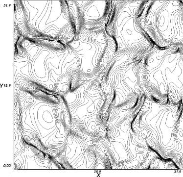
Figure 2: Slice through the $x$-$y$ plane at the centre of the simulation box at $t=6$ showing the isolines of the magnetic field magnitude. Contours have uniform spacing of $0.5$ with $B_{\rm min}=0.5$ and $B_{\rm max}=13$. The regions of strongest field are found in the regions of higher density.

3.3 Results and Discussion I

Initialising the fields using the parameters described in sections 3.1 and 3.2, the development of the root mean squared parallel and perpendicular components of the magnetic field is plotted in Figure 1. Since the plasma starts from rest, the energy input at the beginning primarily goes into kinetic energy of the background fluid and no field growth is observed. After this brief initial stage, at approximately $t=1$, the magnetic field starts to grow at close to the linear growth rate $\gamma_{\rm max}$. The energy in the perpendicular magnetic field eventually overtakes that of the parallel field but continues to grow at the same rate. As the amplitude of the unstable modes approaches that of the mean field, cavity structures similar to those observed in the simulations of Bell (2004) start to appear. The development of these cavities is driven by the Lorentz force exerted on the circular/elliptical modes by the return current. The expansion of each cavity is hindered by the growth of neighbouring cavities and dense regions are formed between them. The frozen-in magnetic field becomes very large inside these cavity walls, as shown in Figure 2.

It is at this point that neglecting the non-linear feedback of the field on the cosmic rays becomes apparent. As discussed in Bell (2005), information is only passed along the direction of the cosmic ray current via tension in the magnetic field lines. However, as the field increases, the cosmic rays themselves would most likely be beamed into the resulting cavities. From the simulations, it is observed that there are no clear coherent structures forming along the direction of the cosmic ray current.

A second difficulty is that vacuum states begin to form within the cavities, and the MHD equations lose their validity. A possible solution to this is to use a highly dissipative scheme, but this reduces the accuracy of the solution. Using such a method the results obtained for the long term evolution of the field are similar to those in Bell (2004), and we do not comment on them.

Since we are primarily concerned with determining diffusion statistics in an amplified field we choose to take a snapshot of the field in the early stages of the non-linear development, at $t=6$. The power spectrum of the field at $t=5$ and $t=6$ is plotted in Figure 3.

\psfrag{pp1}[Bl][Bl][1.0][+0]{$kL$}\psfrag{pp2}[Bl][Bl][1.0][-0]{P(k)}\psfrag{pp3}[Bl][Bl][1.0][-0]{$t=5$}\psfrag{pp4}[Bl][Bl][1.0][-0]{$t=6$}\includegraphics[width=138.76157pt,angle={-90}]{./powerspec.eps}

Figure 3: Logarithmic plot of the power spectrum in the amplified field at times $t=5$ and $t=6$. The spectrum at large $k$ is a power law with $P(k)=k^{-s}$, with $s\approx 7.5$ at $t=5$ and $s\approx 5$ at $t=6$. The turnover in the spectrum moves to smaller $k$ as the parallel component of the field increases.

In the shock frame, the amplified field is advected towards the shock. It is expected that lower energy particles are confined closer to the shock by the turbulence produced further upstream by the cosmic rays which can diffuse further from the shock. We determine the transport properties for relativistic protons in a static amplified field taken at $t=6$.

4 Cosmic Ray and Field Line Transport in Turbulent Field

We now discuss the first results of cosmic-ray transport in a turbulent field resulting from the non-resonant instability of Bell (2004) as described in Section 2. In particular, we investigate how the transport properties differ from the Bohm diffusion limit. Much work has been done on this topic numerically by  (Giacalone & Jokipii, 1994, 1999; Casse, Lemoine & Pelletier, 2002, for example) but in all cases an a priori field was assumed. However, the field we use has been determined self-consistently.

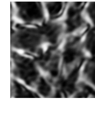
Figure 4: A comparison of the fields after being passed through the low power filter. The same large scale structure maintained quite well between the filtered field (left) and MENDOZA’s field (right).

To determine the statistical transport properties of the amplified field we have developed the code “LYRA” (O’Sullivan et al., 2008). LYRA assumes a Fourier mode description of a static magnetic field as described in Section 3.1. However, MENDOZA represents the magnetic field at a finite number of mesh points (in our case, at $512^{3}$ uniformly spaced points). We convert the field into a continuous Fourier mode representation by taking a Fourier transform and importing the 5000 highest power real modes into LYRA. In the particular case considered here, passing the field through what amounts to a low-power filter results in a loss of $16\%$ of the power in the field. Any lost power is returned to the field by rescaling the included modes accordingly. Figure 4 provides a comparative illustration of the pre-processed field generated by MENDOZA and the filtered field read in by LYRA for the particle transport simulations. As can be seen, the overall large scale structure of the field is maintained quite well, but there is a certain amount of smoothing of the sharper features. However, the continuous description of the field provided by the Fourier transform is more practical than a piecewise constant mesh for the purposes of integrating particle trajectories. The resulting field is also divergence free. We can not be certain that the spreading of the field inside the cavity walls does not affect the final results, but in the current work the Fourier description makes the computations much simpler. We will address this issue in future work.

Another important limitation introduced by importing the field from a periodic grid representation is that while, in theory, we have access to an arbitrarily large dynamic range, the field will remain periodic on the relatively small scale of the parent field. It is important to consider this point when interpreting results displaying any similarity on scales corresponding to the periodicity of the field.

With the field described in this manner, the equations of motion are integrated using the Burlisch-Stoer method (Press et al., 1992). In the case of field lines, the equation to be integrated is $\mbox{d}\mathbf{r}/\mbox{d}s=\mathbf{B}/B$. For protons, the governing equations are

$$\frac{{\rm d}\gamma{\bf v}}{{\rm d}t}=e{\bf v\times B},$$ (22)

and

$$\frac{{\rm d}{\bf r}}{{\rm d}t}={\bf v}.$$ (23)

When integrating the equations of motion for protons, the tolerances in the integrator are set to conserve energy to $\,\raisebox{-1.72218pt}{$\stackrel{{\scriptstyle<}}{{\scriptstyle\sim}}$}\,1\%$ over $1000/2\pi\omega_{\rm g}^{-1}$ where $\omega_{\rm g}^{-1}\equiv 2\pi r_{\rm g}$. We determine the statistical transport properties for 9 different energy values ranging from $\gamma=10^{3}$ to $\gamma=4\times 10^{5}$. For each value, an ensemble of 2000 particles is initialised with random starting positions and pitch angles. Using the $t=6$ field snapshot described in the previous section, with magnetic field simulation units expressed in terms of a $3\mu$G ISM field value, we carry out particle transport simulations using LYRA.

4.1 Results and Discussion II

To investigate the properties of the field lines themselves 2000 field lines are integrated, and the mean square perpendicular displacement along each field line is calculated. The magnetic diffusivity $D\equiv\langle\Delta x^{2}\rangle/2s$, where $s$ is the distance along a field line, is plotted in figure 5. Since the fastest growing modes are circularly polarised, the field lines are helical, although the guiding centre wanders about the $x$-$y$ plane as it moves along the $z$-axis. The parallel diffusivity is essentially ballistic ($D_{\|}\propto s$).

\psfrag{pp1}[Bl][Bl][1.0][+0]{$D_{\perp}$}\psfrag{pp2}[Bl][Bl][1.0][-0]{$s$}\includegraphics[width=186.45341pt]{./DmPerp.eps}

Figure 5: The Perpendicular magnetic diffusivity plotted against distance along a field line. Both in in units of box lengths.

We numerically determine the statistical average diameter of the helices by iterating over the same 2000 field lines, and approximating the diameter of each revolution. In what follows, all length units are normalised to simulation box lengths. The root mean square diameter of the helices is $d=0.148$ which is an important length scale in the study of the fields properties. The peak in the perpendicular magnetic diffusivity is located at $s=0.273$. Using this value and setting the perpendicular displacement equal to the root mean square diameter gives $D_{\perp}=0.08$ which is in reasonable agreement with the experimentally determined peak at approximately $D_{\perp}=0.057$, as shown in figure 5.

\psfrag{pp1}[Bl][Bl][1.0][+0]{$t$}\psfrag{pp2}[Bl][Bl][1.0][-0]{ $\frac{\langle\Delta z^{2}\rangle}{2\Delta t}$}\includegraphics[width=138.76157pt,angle={-90}]{./kpll.eps}

Figure 6: $\frac{\langle\Delta z^{2}\rangle}{2\Delta t}$ at t=6 showing times for super-diffusive regime in units of box-lengths squared per Larmor time. Lines correspond to gamma factors (from bottom to top at $\Delta t=100$) $\gamma=4\times 10^{3},~{}10^{4},~{}2\times 10^{3},~{}2\times 10^{4},~{}10^{3}$. Time units are Larmor times for a $\gamma=10^{4}$ particle. Note these lines continue to asymptotic values and we show only the early evolution to demonstrate the super-diffusive behaviour.

The mode with the fastest growth rate has a wavelength similar to the gyroradius of protons with a particle gamma factor of $\gamma\approx 2\times 10^{4}$. We focus on the transport properties close to this value. Particles with $\gamma$ much less or greater than this have mean free paths close to a cell width or box length respectively.

We interpret these results in terms of the diffusion coefficients for the actual particle trajectories determined from LYRA. The parallel and perpendicular diffusion coefficients are determined by averaging over a large ensemble of particles

$$\kappa_{\|}\equiv\lim_{\Delta t\rightarrow\infty}\frac{\langle\Delta z^{2}\rangle}{2\Delta t}$$ (24)

$$\kappa_{\bot}\equiv\lim_{\Delta t\rightarrow\infty}\frac{\langle\Delta x_{\bot}^{2}\rangle}{2\Delta t}$$ (25)

Note that the $\kappa_{\|}$ and $\kappa_{\perp}$ refer to parallel and perpendicular directions with respect to the initial field, whereas in the $t=6$ snapshot of the field the perpendicular component already dominates, as is evident from Figure 1.

The initial evolution of the particle trajectories are governed by the field line statistics. Figure 6 and Figure 7 plot the early parallel and perpendicular diffusion respectively, showing an initially super diffusive regime, with a peak in the perpendicular value for the lower energy particles occurring at approximately 5 $\omega_{\rm g}^{-1}$. Inserting this values into Eq. (25) and equating to the experimental peak value $\sim 0.0015$, gives an estimate for the root mean square perpendicular displacement at the peak, $\sqrt{\langle\Delta x_{\bot}^{2}\rangle}=0.08$. This value is also in agreement with the statistical mean radius of the helices. For higher energy particles the Larmor radius of a particle becomes comparable to or larger than the average diameter, and the peak time differs from this value. These particles are not trapped to individual field lines and must travel a greater distance before becoming diffusive.

\psfrag{pp1}[Bl][Bl][1.0][+0]{$t$}\psfrag{pp2}[Bl][Bl][1.0][-0]{ $\frac{\langle\Delta x_{\bot}^{2}\rangle}{2\Delta t}$}\includegraphics[width=138.76157pt,angle={-90}]{./kperp.eps}

Figure 7: $\kappa_{\perp}$ at $t=6$ showing times for super-diffusive regime in units of box-lengths squared per Larmor time. Lines correspond to gamma factors (from bottom to top) $\gamma=10^{3},~{}2\times 10^{3},~{}4\times 10^{3},~{}10^{4},~{}2\times 10^{4},~{}4\times 10^{4}$. Time units are Larmor times for a $\gamma=10^{4}$ particle .

The asymptotic values of the diffusion coefficients, after the non-diffusive regimes, are plotted in figure 8. It is clear that $\kappa_{\|}<\kappa_{\bot}<\kappa_{\rm Bohm}$, in the energy range corresponding to $k_{\rm max}r_{\rm g}\approx 1$. In a uniform field, quasi-linear theory predicts $\kappa_{\bot}<\kappa_{\rm Bohm}<\kappa_{\|}$. However, in the highly non-uniform field produced by the non-resonant instability, the experimentally determined transport properties are much more complicated. Nevertheless, the parallel diffusion coefficient, along with the shock speed, defines the residence and acceleration timescales. While the simulations presented in this paper do not include resonant wave excitation, which would act to reduce the diffusion coefficients even further, it is worthwhile speculating on the effects that our results would have on the shape of the CR spectrum and the rate of the shock acceleration process. The acceleration rate defined by Lagage & Cesarsky (1983) is proportional to the magnetic field strength. Amplification of the magnetic field, as in the snapshot we selected, above interstellar medium values would therefore increase the maximum energy limit given by Lagage & Cesarsky (1983). Inclusion of resonant wave excitation and application to the case of a circumstellar wind would increase that limit even further (Bell & Lucek, 2001) as, of course, would a higher saturation level of the non-resonant waves.

\psfrag{pp1}[Bl][Bl][1.0][+0]{$\kappa_{\|}/\kappa_{\rm Bohm}$}\psfrag{pp3}[Bl][Bl][1.0][-0]{$\kappa_{\perp}/\kappa_{\rm Bohm}$}\psfrag{pp2}[Bl][Bl][1.0][-0]{$\gamma$}\includegraphics[width=203.80193pt]{./koverkb.eps}

Figure 8: $\kappa_{\|}/\kappa_{\rm Bohm}$ (solid) and $\kappa_{\bot}/\kappa_{\rm Bohm}$ (dashed) with $\kappa_{\rm Bohm}$ evaluated in a $3\mu{\rm G}$ field, at t=6.

Turning to the shape of the spectrum, at a strong shock front with a compression ratio of four the standard result that $f\propto p^{-4}$ applies provided that particles are isotropised and that their motion becomes diffusive within a residence time either side of the shock (Duffy et al., 1996). In our simulations the isotropisation is very rapid, on the timescale of one to two Larmor times. However, the parallel motion only becomes fully diffusive after almost ten Larmor times and is super-diffusive ($<\Delta x^{2}>\propto t^{\beta}$ where $\beta>1$) up to that point. It has been shown (Kirk, Duffy & Gallant, 1996) that if particle crossings happen on a timescale below that required for diffusive transport then the resulting spectrum will be a power law given by $f\propto p^{-(5-\beta)}$ provided the distribution remains close to isotropy. In our super-diffusive case, $\beta>1$, this would imply a spectrum that is harder than the diffusive shock acceleration result. Therefore, our results are consistent with the rapid acceleration of a relatively hard spectrum,but clearly more work needs to be done on resonant wave excitation and overall dynamical range before drawing definitive conclusions.

5 Conclusions

We have reported on the results from high-resolution MHD simulations of the non-resonant current driven instability. The long term evolution of the field is still uncertain, as the non-linear development leads to very low density cavities in the absence of significant numerical dissipation. To overcome this, future simulations should include a non-linear feedback on the cosmic rays perhaps using a hybrid code, similar to the work of Lucek & Bell (2000), or by performing large-scale particle in cell (PIC) simulations. To this end, Riquelme & Spitkovsky (2007) have performed 2D PIC simulations of the relativistic generalisation of the Bell-type instability (Reville, Kirk, & Duffy, 2006) and preliminary results show that the field saturates with both the perpendicular and parallel magnetic field well in excess of the initial mean value. On the other hand, Niemiec & Pohl (2007) have reported on 3D PIC simulations, with initial parameters chosen such that the non-resonant mode is expected to be observed. However, the filamentation instability dominates the growth of the field and the perturbations do not grow much beyond the initial mean field value. The results of PIC simulations of this instability remain inconclusive. The simulations of Riquelme & Spitkovsky (2007) are promising in that they do show the development of extended filaments, as predicted in Bell (2005), and this should be important for future investigations of particle transport.

In recent years, magnetic field amplification has become a popular mechanism for accelerating cosmic rays beyond the Lagage-Cesarsky limit. We present here, the first attempt at investigating self-consistently the particle diffusion statistics in a self-excited magnetic field. The observed diffusion is anisotropic ($\kappa_{\|}\neq\kappa_{\perp}$), with the low energy particles’ diffusion being largely determined by the field statistics. Thus at low energies $\kappa_{\|}>\kappa_{\perp}$. However, on length scales similar to the wavelength of the helical modes, motion parallel to the shock normal is more diffusive. At high energies the diffusion seems to be energy independent perpendicular to the initial field direction, but scales as $\gamma^{2}$ parallel. This follows naturally since there are few waves with scalelength comparable to the gyroradii of these particles in our simulation box. However, the simulations do achieve sub-Bohm diffusion with only modest amplification of the effective ambient field.

It is clear that in the presence of non-linear waves the diffusion properties of particles differ greatly from the standard picture. Based on the results presented here it is difficult to say if the super-diffusive or sub-diffusive regimes will have a significant effect on the shape of the spectrum. An estimation of the acceleration timescale of cosmic rays is beyond the scope of this paper, nevertheless we have demonstrated that self-excited turbulence does reduce the diffusion coefficient of the cosmic rays and is therefore likely to lead to acceleration beyond the Lagage-Cesarsky limit.

References

- Batchelor (1982) Batchelor G.K., 1982, The Theory of Homogeneous Turbulence, Cambridge University Press
- Bell (2004) Bell A.R., 2004, Mon. Not. R. Astron. Soc. , 353, 550
- Bell (2005) Bell A.R., 2005 , Mon. Not. R. Astron. Soc. , 358, 181
- Bell & Lucek (2001) Bell A.R., Lucek S.G., 2001, Mon. Not. R. Astron. Soc. 321, 433
- Blasi (2002) Blasi P., 2002, Astroparticle Physics, 16, 429
- Casse, Lemoine & Pelletier (2002) Casse F., Lemoine M., Pelletier G., 2002, Phys. Rev. D, 65, 3002
- Dedner et al. (2002) Dedner A., Kemm F., Kröner D., Munz C.-D., Schnitzer T. and Wesenberg,M.A., 2002, J.Comp.Phys. 175, 645
- Duffy et al. (1996) Duffy P., Kirk J.G., Gallant Y.A., Dendy R.O., 1996, Astronomy & Astrophysics, 302, L21
- Eichler (1979) Eichler D., 1979, Astrophysical Journal, 229, 419
- Giacalone & Jokipii (1994) Giacalone J., Jokipii J. R., 1994, Astrophysical Journal, 430, L137
- Giacalone & Jokipii (1999) Giacalone J., Jokipii J. R., 1999, Astrophysical Journal, 520, 204
- Falle et al. (1998) Falle S.A.E.G., Komissarov S.S., Joarder P., 1998, Mon. Not. R. Astron. Soc. , 297, 265
- Kirk, Duffy & Gallant (1996) Kirk J.G., Duffy P., Gallant Y.A., 1996, Astronomy & Astrophysics 314 1010
- Lagage & Cesarsky (1983) Lagage P.O., Cesarsky C.J., 1983, Astronomy & Astrophysics 125 249
- Lucek & Bell (2000) Lucek S. G., Bell A. R., 2000, Mon. Not. R. Astron. Soc. 314, 65
- McKenzie & Völk (1982) McKenzie J.F., Völk H.J., 1982 Astronomy & Astrophysics 116, 191
- Melrose (2005) Melrose D., 2005, AIPC, 781, 135
- Niemiec & Pohl (2007) Niemiec J., Pohl M., 2007, AIPC, 921, 405
- O’Sullivan & Downes (2007) O’Sullivan S., Downes T.P., 2007, Mon. Not. R. Astron. Soc. 376, 4
- O’Sullivan et al. (2008) O’Sullivan S., Duffy P., Blundell K.M., Binney J., submitted to Phys. Rev. D.
- Press et al. (1992) Press, W. H., Teukolsky, S. A., Vetterling, W. T., Flannery, B. P., 1992, Numerical recipes in C, Cambridge: University Press
- Reville et al. (2007) Reville B., Kirk J.G., Duffy P., O’Sullivan S. 2007, Astronomy & Astrophysics 475, 435
- Reville, Kirk, & Duffy (2006) Reville, B., Kirk, J. G., & Duffy, 2006, P., Plasma Physics and Controlled Fusion, 48, 1741
- Riquelme & Spitkovsky (2007) Riquelme M., Spitkovsky A., 2007, HEPRO conference proceedings
- Tóth (2000) Tóth G., 2000, Journal of Computational Physics, 161, 605
- Zank et al. (2006) Zank G. P., Li G., Florinski V., Hu Q., Lario D., Smith C. W., 2006, J. Geophys. Res., 111, A06108