Detecting photon-photon scattering in vacuum at exawatt lasers
Abstract
In a recent paper, we have shown that the QED nonlinear corrections imply a phase correction to the linear evolution of crossing electromagnetic waves in vacuum. Here, we provide a more complete analysis, including a full numerical solution of the QED nonlinear wave equations for short-distance propagation in a symmetric configuration. The excellent agreement of such a solution with the result that we obtain using our perturbatively-motivated Variational Approach is then used to justify an analytical approximation that can be applied in a more general case. This allows us to find the most promising configuration for the search of photon-photon scattering in optics experiments. In particular, we show that our previous requirement of phase coherence between the two crossing beams can be released. We then propose a very simple experiment that can be performed at future exawatt laser facilities, such as ELI, by bombarding a low power laser beam with the exawatt bump.
pacs:
12.20.Ds, 42.50.Xa, 12.20.FvI Introduction
Radiative corrections in Quantum Electrodynamics (QED) have been studied for 70 years, both theoretically and experimentallyWeinberg . Nevertheless, in the last decade they have gained an increasing interest, following the extraordinary advancements in the fields of Quantum and Nonlinear Optics. On one hand, it has been noted that a fundamental uncertainty in the number of photons is unavoidably generated by QED radiative correctionstommasini0203 , eventually competing with the experimental errors. On the other hand, the interchange of virtual electron-positron pairs can produce classically forbidden processes such as photon-photon scattering in vacuum.
Although it is a firm prediction of QED, photon-photon scattering in vacuum has not yet been detected, not even indirectly. The rush for its discovery is then wide open. A hammer strategy will be to build a photon-photon colliderphcollider , based on an electron laser producing two beams of photons in the range (i.e., having wavelengths in the range of a few ). This will maximize the cross section for the process. A second approach will be to perform experiments using ultrahigh power optical lasers, such as those that will be available in the near futuremourou06 , in such a way that the high density of photons will compensate the smallness of the cross section. In this case, the photon energies are well below the electron rest energy, and the effect of photon-photon collisions due to the interchange of virtual electron-positron pairs can be expressed in terms of the effective Euler-Heisenberg nonlinear LagrangianHalpern ; Heisenberg . This modifies Maxwell’s equations for the average values of the electromagnetic quantum fieldsmckenna and affects the properties of the QED vacuumklein .
Ultra intense photon sources are available thanks to the discovery of chirped pulse amplification (CPA)strickland85 in the late 80’s and optical parametric chirped pulse amplification (OPCPA) dubietis92 in the 90’s. These techniques opened the door to a field of research in the boundary between optics and experimental high-energy physics, where lots of novelties are expected to come in the next years. In fact, several recent works propose different configurations that can be used to test the nonlinear optical response of the vacuum, e.g. using harmonic generation in an inhomogeneous magnetic fieldding92 , QED four-wave mixing4wm , resonant interactions in microwave cavitiesbrodin , or QED vacuum birefringenceAlexandrov which can be probed by x-ray pulsesxray , among othersothers .
In a recent Letterprl99 , we have shown that photon-photon scattering in vacuum implies a phase correction to the linear evolution of crossing electromagnetic waves, and we have suggested an experiment for measuring this effect in projected high-power laser facilities like the European Extreme Light Infrastructure (ELI) projectELI for near IR radiation. Here, we provide a more complete analysis, including a full numerical solution of the QED nonlinear wave equations for short-distance propagation in a symmetric configuration. The excellent agreement of such a solution with the result that we obtain using a perturbatively-motivated Variational Approach is then used to justify an approximation that can be applied in a more general case. This allows us to find the most promising configuration for the search of photon-photon scattering in optics experiments. In particular, we show that our previous requirement of phase coherence between the two crossing beams can be released. We then propose a very simple experiment that can be performed at future exawatt laser facilities, such as ELI, by bombarding a low power laser beam with the exawatt bump. The effect of photon-photon scattering will be detected by measuring the phase shift of the low power laser beam, e.g. by comparing it with a third low power laser beam. This configuration is simpler, and significantly more sensitive, than the one proposed in our previous paper. Even in the first step of ELI, we find that the resulting phase shift will be at least , which can be easily measured with present technology. Finally, we discuss how the experimental parameters can be adjusted to further improve the sensitivity.
The paper is organized as follows:
In Section II, following Ref. prl99 , we present the nonlinear equations that replace the linear wave equation when the QED vacuum effect is taken into account.
In Section III, we consider a linearly polarized wave, describing the scattering of two counterpropagating plane waves that have the same intensity and initial phase at the origin (symmetric configuration). In this case, we perform a numerical simulation for short-distance propagation, which provides the first known solution to the full QED nonlinear wave equation.
In Section IV, we study the same configuration as in Sect. III by using a Variational Approximation. This allows us to obtain an analytical solution which is valid even for a long evolution. After showing that this variational solution is in good agreement with the numerical simulation of Sect. III, we give a method to study different configurations that cannot be integrated numerically in a simple and direct way.
In Section V, we apply our Variational Approximation to the case of the scattering of a relatively low power wave with a counterpropagating high power wave, both traveling along the axis. We allow an arbitrary initial phase relation between the two waves, and obtain an analytical solution showing a phase shift of the low power wave.
In Section VI, we discuss the possibility of detecting photon scattering by measuring the phase shift of two counterpropagating waves at ELI. We show that an asymmetric configuration, in which only one high power laser beam is used and the phase is measured on the low power laser beam, is not only simpler to realize, but it also gives a better sensitivity than the symmetric configuration. The resulting proposed experiment will then allow to detect photon-photon scattering as originated by QED theory.
In Section VII, we resume our conclusions, and discuss why we think that our proposed experiment will be the simplest and most promising way to detect photon-photon scattering with optical measurements in the near future.
II The nonlinear equation for linearly polarized waves in vacuum
In this section we introduce the equations that govern the evolution of the electromagnetic fields E and B when the QED effects are taken into account. We assume that the photon energy is well below the threshold for the production of electron-positron pairs, . This means that we will only consider radiation of wavelengths , which is always the case in optical experiments. In this case, the QED effects can be described by the Euler-Heisemberg effective Lagrangian densityHeisenberg ,
| (1) |
being
| (2) |
the linear Lagrangian density and and the dielectric constant and the speed of light in vacuum, respectively. As it can be appreciated in Eq. (1), QED corrections are introduced by the parameter
| (3) |
This quantity has dimensions of the inverse of an energy density. This means that significant changes with respect to linear propagation can be expected for values around , corresponding to beam fluxes with electromagnetic energy densities given by the time-time component of the energy-momentum tensor
| (4) |
While such intensities may have an astrophysical or cosmological importance, they are not achievable in the laboratory. The best high-power lasers that are being projected for the next few decades will be several orders of magnitude weaker, eventually reaching energy densities of the order mourou06 . Therefore, we will study here the “perturbative” regime, in which the non-linear correction is very small, . As we shall see, even in this case measurable effects can be accumulated in the phase of beams of wavelength traveling over a distance of the order . Thus, current sensitive techniques could be used to detect traces of QED vacuum nonlinearities.
Once the electromagnetic fields are expressed in terms of the four-component gauge field as and , the equations of motion are given by the Variational Principle:
| (5) |
where is the QED effective action. Instead of studying the resulting equations for the fields and , that can be found in the literaturemckenna ; variational , for the present purposes it is more convenient to consider the equations for the gauge field components . In general, these four equations cannot be disentangled. However, after some straightforward algebra it can be seen that they admit solutions in the form of linearly polarized waves, e.g. in the direction, with and , provided that: the field does not depend on the variable (a transversality condition) and satisfies the single equation:
| (6) |
where we have used the convention for the metric tensor. In non-relativistic notation, Eq. (6) can be written as
| (7) | |||
where , and .
Hereafter, we will restrict our discussion to this case of linearly-polarized solution. The orthogonality relation is then automatically satisfied, and the effective Lagrangian Eq. (1) reduces to . Note that the plane-wave solutions of the linear Maxwell equations, such as , where is a constant, and , are still solutions of Eq. (6). However, we expect that the non-linear terms proportional to , due to the QED correction, will spoil the superposition principle.
III A numerical solution of the full nonlinear equation (symmetric configuration)
In general, the numerical solution of a nonlinear wave equation such as Eq. (7) is a formidable problem. In fact, it is of an higher order (and is much more complicated) than the nonlinear Shrödinger equation in three dimensions, which is nevertheless a highly nontrivial and rich systemnlse . There are two main difficulties in dealing with Eq. (7). First of all, the direct numerical integration is practically impossible when the integrating interval is much larger than the wavelength. Second, one has to find convenient boundary conditions.
In this section, we will study a particular configuration for which a numerical solution of the full nonlinear equation Eq. (7) can be found. Let us first consider two counter-propagating plane waves that travel along the -axis, for simplicity having the same phase at the space-time origin. The corresponding analytical solution of the linear wave equation (that can be obtained by setting in Eq. (7)) would be
where is a constant amplitude, is the wave vector, and is the angular frequency. It is easy to see that Eq. (III) can also be considered as the analytical solution of the linear wave equation satisfying the boundary conditions
| (9) | |||||
where for convenience we chose as the integration interval a ‘small’ cuboid of time-dimension and space-dimension . With such a choice, the linear wave equation can also be integrated numerically, obtaining a result that coincides (within the numerical error) with the analytical one.
Of course, in the case of the linear equation this result is trivial. However, we will use it here as a guide in order to find a solution of the nonlinear Eq. (7). In fact, although we do not know any analytical solution of the latter equation, we can find its numerical solution that satisfies the same boundary conditions of Eq. (9) using the same small cuboid as the integration interval.
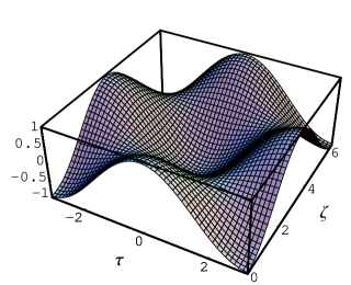

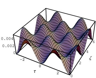
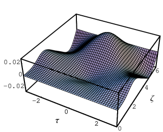
With these conditions, the result of the numerical integration of Eq. (7) is shown in Figs. 1 and 2 for a choice of parameters such that . The corresponding energy density, obtained as
is plotted in Fig. 3.
As far as we know, this is the first time that a numerical solution of the full nonlinear wave equation Eq. (7) is obtained. Of course, it corresponds to a very simple particular case and a short space-time evolution. However, we will see later that this solution will allow us to reach very important conclusions and prove the viability of useful approximation methods.
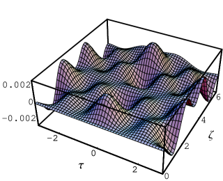
For the moment, we note that our numerical solution, as given in Figs. 1, 2 and 3, shows an oscillatory behaviour. However, the time-average of the energy density turns out to be approximately constant along the -evolution, giving . As we have discusses above, this value of the product is several order of magnitude larger than what can be achieved in the laboratory in the next decades. Of course, we will use realistic values of when we will present our proposals of experiments in the last sections. For the moment, it is interesting to note that even such an enormous energy density is still small enough so that the effect of the nonlinear terms gives a small correction to the linear evolution in the short distance. In fact, we see from Fig. 4 that the relative difference between the linear and the nonlinear evolution, in our integration interval which is of the order of the wavelength, is of the order of few percent, i.e. of the same order than the adimensional parameter . This result is not surprising, and will provide a justification for the perturbatively-motivated variational approach that we will use in the next sections.
.
However, from Fig. 4 itself, we can also appreciate that the difference between the linear and nonlinear behaviour tends to increase along the evolution, so that it can be expected that it will eventually become large after a distance much larger than the wavelength. In the next section, we will see an analytical argument that confirms this expectation.

Finally, in Fig. 5 we compare the -evolution of the solutions and in a greater detail for values of around the second zero of the solutions. We see that anticipates , and the corresponding phase shift can be evaluated numerically if we define an effective wave vector component by computing the value corresponding to , and setting . The numerical determination of the zero gives , so that . We will provide a full explanation for this result in the following section.
IV Variational approximation (symmetric configuration)
Although it can be considered as an interesting achievement due to its simplicity and lack of previous approximations, in practice the numerical solution that has been discussed above can only be obtained in the special configuration of two counter-propagating, in-phase waves, and for short propagation (of the order of the wavelength). In this section, we will consider the same configuration, and we will look for a variational approximation that will provide an analytical solution which is valid even for a long evolution. After showing that this variational solution is consistent with the numerical one of the previous section, we will obtain a method to study different configurations that cannot be integrated numerically in a simple and direct way.
We will thus consider again the two counterpropagating waves, that would be described by Eq. (III) in the linear case. Note that any of the two crossing waves, and , when taken alone, would be a solution of both the linear and non-linear equations, provided that . However, their superposition would only solve the linear equations of motion.
As we discussed in Ref. prl99 , in all the experimental configurations that can be studied in the present and the near future, the product will be so small, that the non-linear correction will act in a perturbative way, progressively modifying the form of as the wave proceeds along the direction. We will therefore make the ansatz
| (11) |
allowing for the generation of the other linearly-independent function (we will take and ). Note that the invariance of Eq. (7) under time reversal guarantees that, if the initial behavior is proportional to , which is even under time inversion, no uneven term proportional to will be generated.
According to the Variational Method, the best choice for the functions and corresponds to a local minimum of the effective action , after averaging out the time-dependence as follows:
| (12) |
The expression that is obtained by this procedure is still quite complicated, due to the presence of the trigonometric functions of multiples of . However, as we shall see below, when this -dependence is much faster than that of the envelop functions and . Therefore, it is a very good approximation to perform the integral in two steps: first, we average over a period, treating and as if they were constant. In this way, we get rid of the trigonometric functions. At this point, we allow again the dependence of the envelop functions. If we call the average action that is obtained by this procedure, we will then minimize it with respect to the functions and by solving the equations y .
After a long but straightforward computation, and neglecting the non-linear terms involving derivatives of the functions and , since they give a smaller contribution as we discussed in Ref. prl99 , these two equations can be written as
| (13) |
and
| (14) |
where is a parameter that describes the leading nonlinear effects.
Now, in the perturbative regime in which is small, we can also neglect the second derivatives in the previous equationsprl99 , so that an (approximate) analytical solution for Eqs. (13) and (14) is given by and . Substituting this result into the variational ansatz (11), and using elementary trigonometry, we obtain
| (15) |
As a result, we find that the phase of the wave is shifted by a term
| (16) |
Note that the solution of Eq. (15) can also be written as
| (17) |
therefore we see that each of two scattering waves is phase shifted according to Eq. (16), due to the crossing with the other wave. A similar behavior can also be found in a nonlinear mediumnl2 , although the analogy cannot be pushed too far, as we have discussed in Ref. prl99 , where we have shown that the vacuum does not present the usual AC Kerr effect.
Note also that the result of Eq. (15) can be stated equivalently by defining a wave vector as , that satisfies a modified dispersion relation, .
In order to make definite numerical predictions, it is convenient to express the amplitude in terms of the energy density, as given by Eq. (III). In our perturbative regime, after time and space average, this gives with a very good approximation. Thus we get , so that the phase shift accumulated after a distance is
| (18) |
We see now that the slow varying envelop approximation was justified as far as .
For the same choice of parameters that was considered in the previous section, , in agreement with the numerical simulation. Thus we get , which is two order of magnitude smaller than . Our approximations can then be expected to be reasonably good even for the extremely large of that we have chosen here. Note also that this corresponds to a value , in agreement with the result that we obtained from the numerical simulation in the previous section.
In Fig. 6 we compare the corresponding analytical solution , given in Eq. (15), with the numerical solution of the QED wave equations that we have found in the previous section. Comparing with Fig. 4, we see that the variational solution is an order of magnitude closer to the numerical simulation than the linear evolution, Eq. (III), that was obtained by completely neglecting the nonlinear terms. This is a significant improvement in such a short distance. However, according to the previous discussion, in the perturbative regime corresponding to small values of the product , the variational solution is expected to be a good approximation even when a longer propagation distance is considered along the -axis. In fact, this expectation is confirmed by Fig. 6 itself, that shows that the error of the variational solution oscillates without any substantial increment in the integration interval. As we have observed in the previous section, this was not the case for the linear solution, which was incresing its error even in the short distances. Of course, this is due to the fact that it does take into account the phase shift, which is the leading effect due to the nonlinear terms according to our Variational Method. On the other hand, the agreement of the variational solution with the numerical simulation can be used as an additional, a posteriori justification for our analytical approach.
V Variational approximation (asymmetric configuration)
In the previous section, we have proved the reliability of a perturbatively-motivated Variational approach in the search for approximate solutions of the QED nonlinear wave equation, Eq. (7) In that case, we studied a symmetric configuration in order to compare the result with the numerical integration of the full equation. With this strong justification in mind, we can now apply the Variational Method to different configurations, that do not allow for a direct integration of the full Eq. (7).
In this section, we will study the case of the scattering of a relatively low power wave with a counterpropagating high power wave, both traveling along the axis. In this case, the main effect will be the modification of the low power beam due to the crossing with the high power one, which would be unaffected in a first approximation.
Using our variational approach, we will describe the high power field by a wave polarized in the direction, having the -component of the vector potential given by
| (19) |
where is an arbitrary phase, describing the unknown phase difference between the two counterpropagating beams. Such a beam is shot against a low power wave that, in the absence of the nonlinear QED terms, would be described by a -component of the vector potential given by , where the constant is related to the intensity of the beam. In other words, the only condition is that the two waves have the same frequency. Photon-photon scattering will then generate a -dependence of and an additional term proportional to in the low power wave, so that
| (20) |
with the initial condition and . Neglecting the effect of the low power beam on the high power wave, we are then lead to the ansatz
| (21) |
According to the Variational Method, we require that the functions and correspond to a local minimum of the effective action , after averaging out the time-dependence as described in Eq. (12). After averaging over the fast dependence on , as discussed in the previous section, and neglecting again the non-linear terms involving derivatives of the functions and , we get the following equations
| (22) |
and
| (23) |
where . Note that Eqs. (22) and (23) are linear, and they do not show any dependence of the initial phase difference between the two beams. Neglecting the second derivatives, for the same reason that were discussed in the previous section, we get the solution and . Note also that this solution is valid for any value of the amplitude of the low power wave, provided that it is much smaller than the amplitude of the high power beam, .
As a result, we find that the low power beam becomes
| (24) |
Taking into account that the average energy density of the high power wave is , we can compute the phase shift accumulated by the low power wave after a distance as
| (25) |
We stress that this result only depends on the energy density of the high power wave, as far as it much larger than that of the low power wave. The initial phase difference is found to be irrelevant.
VI Proposal of an experiment
We can now discuss the possibility to test the non-linear properties of the QED vacuum by measuring small phase changes in one of two crossing laser beams at a very high power laser facility. In the previous sections, we have studied the leading QED nonlinear effect on two counterpropagating waves traveling in the -direction. We have considered two different configurations: a symmetric one, in which both waves are high power waves with the same initial phase and amplitude; and an asymmetric configuration, in which only one the two waves is high power, and they do not need to be in phase. Of course, the second configuration is easier to be produced experimentally. Moreover, as we shall discuss below, it leads to a phase shift which is (at least) twice higher than that which could be obtained from the symmetric configuration, for the same experimental facility.
In fact, the total energy density achievable in the symmetric configuration is the space-time average due to both waves, that have to be obtained from the same original high power pulse through a beam splitter. Therefore, even if we neglect the energy loss when the beams split, the value of in Eq. (25) is roughly the same than that of the single high power beam of Eq. (18). Therefore, the asymmetric configuration of section V produces a phase shift which is roughly twice than that of the symmetric configuration that we have discussed.
Therefore, we will propose the following experimental setup, which in our opinion will provide the simplest and most effective way to look for optical effects of photon-photon scattering in future exawatt laser facilities. A common laser pulse is divided in two beams, A and B, one of which (say A) crosses at a a very high power beam. As a result, the central part of the distribution of the beam A has acquired a phase shift with respect to beam B, that has propagated freely. In a experiment corresponding to the parameters of the ELI project in its first step we have pulses of wavelength , intensity and duration which are focused in a spot of diameter . From Eq. (25), this results in a phase shift for beam A, which can be resolved comparing with the beam B which was not exposed to the effects of QED vacuum. Current techniques like spectrally resolved two-beam coupling, which can be applied for ultrashort pulseskang97 , can be used to this purpose.
It is interesting to note that the sensitivity of this method for the detection of photon-photon scattering may be enhanced by a suitable choice of the combination of the intensity , the wavelength and the time duration that enter in Eq. (25). In fact, taking into account that , Eq. (25) implies that the most sensitive experimental configuration will be that having the maximum value of the combination .
Comparing to other alternatives like x-ray probing of QED birefringence, our system does not need an extra free electron laser and the power requirements of the system are only one order of magnitude higher. Moreover, the measurement of the ellipticity and the polarization rotation angle in birefringence experiments is not yet possible with current technology. Other techniques like four-wave mixing processes4wm require the crossing of at least three beams, with the corresponding alignment problems and the rest of the requirements are similar to our proposal. Moreover, the present result also improves significantly the one arising for two high-power waves that we discussed in Ref. prl99 .
VII Conclusions
In this paper, we have studied the nonlinear wave equations that describe the electromagnetic field in the vacuum taking into account the QED corrections. In particular, we have studied the scattering of two waves in a symmetric and an asymmetric configuration. In the first case, we have found a full numerical solution of the QED nonlinear wave equations for short-distance propagation. We have then perfomed a variational analysis and found an analytical approximation which is in very good agreement with our numerical solution, but can also be used for long distance propagation. We have then studied an aymmmetric configuration corresponding to the head-on scattering of a ultrahigh power with a low power laser beam and argued that it is the most promising configuration for the search of photon-photon scattering in optics experiments. In particular, we have shown that our previous requirement of phase coherence between the two crossing beams can be released. We have then proposed a very simple experiment that can be performed at future exawatt laser facilities, such as ELI, by bombarding a low power laser beam with the exawatt bump. Photon-photon scattering will then be observed by measuring the phase shift of the low power laser beam, e.g. by comparing with a third low power laser beam. This configuration is simpler, and significantly more sensitive, than that proposed in our previous paper. Even in the first step of ELI, we have found that the resulting phase shift will be at least , which can be easily measured with present technology. Finally, we have discussed how the experimental parameters can be adjusted to further improve the sensitivity.
Acknowledgments.- We thank Miguel Ángel García-March, Pedro Fernández de Córdoba, Gérard Mourou and Mario Zacarés for useful discussions. One of the authors (D. T.) would also like to thank the whole InterTech group at the Universidad Politécnica de Valencia for its warm hospitality. This work was partially supported by contracts PGIDIT04TIC383001PR from Xunta de Galicia, ACOMP07/221 from Generalitat Valenciana, FIS2007-29090-E, FIS2007-62560, FIS2005-01189 and TIN2006-12890 from the Government of Spain.
References
- (1) S. Weinberg, The Quantum Theory of Fields, Vol. I, Cambridge University Press (1995).
- (2) D. Tommasini, JHEP 07, 039 (2002); Opt. Spectrosc. 94, 741 (2003).
- (3) I. Ginzburg, G. Kotkin, V. Serbo, V. Telnov, Pizma ZhETF 34, 514 (1981); JETP Lett. 34, 491 (1982).
- (4) O. Halpern, Phys. Rev. 44, 855 (1933); H. Euler, Ann. Physik 26, 398 (1936).
- (5) W. Heisenberg and H. Euler, Z. Physik 98, 714 (1936).
- (6) J. McKenna and P. M. Platzman, Phys. Rev. 129, 2354 (1963).
- (7) J. J. Klein and B. P. Nigam, Phys. Rev. 135, B1279 (1964)
- (8) G. A. Mourou, T. Tajima, and S. V. Bulanov, Rev. Mod. Phys. 78, 310 (2006).
- (9) A. D. Strickland and G. Mourou, Opt. Comm. 56, 212 (1985); P. Maine and G. Mourou, Opt. Lett. 13, 467 (1988).
- (10) A. Dubietis, G. Jonusauskas, and A. Piskarskas, Opt. Comm 88, 437 (1992).
- (11) Y. J. Ding and A. E. Kaplan, J. Nonlinear Opt. Phys. Mater. 1, 51 (1992).
- (12) S. L. Adler, Ann. Phys. 67, 599 (1971); F. Moulin and D. Bernard, Opt. Comm. 164, 137 (1999); E. Lundstrom et al., Phys. Rev. Lett. 96, 083602 (2006).
- (13) G. Brodin, M. Marklund, and L. Stenflo, Phys. Rev. Lett. 87, 171801 (2001).
- (14) E. B. Aleksandrov, A. A. Anselm, and A. N. Moskalev, Zh. Eksp. Teor. Fiz. 89, 1181 (1985)[Sov. Phys. JETP 62, 680 (1985)].
- (15) T. Heinzl et al., Opt. Comm. 267, 318 (2006); A. Di Piazza et al., Phys. Rev. Lett., 97, 083603 (2006).
- (16) M. Soljačić and M. Segev, Phys. Rev. A 62, 043817 (2000); M. Marklund and P. K. Shukla, Rev. Mod. Phys. 78, 591 (2006), and references therein.
- (17) A. Ferrando, H. Michinel, M. Seco, and D. Tommasini, Phys. Rev. Lett., 99, 150404 (2007).
- (18) Information about the ELI project is available at the official web site http://www.extreme-light-infraestructure.eu.
- (19) G. Brodin, et al. Phys. Lett. A 306, 206 (2003).
- (20) R. de la Fuente R, O. Varela, and H. Michinel, Opt. Comm. 173, 403 (2000); V. M. Pérez-García et al., J. Opt. B 2, 353 (2000).
- (21) J. Babarro, et al. Phys. Rev. A 71, 043608 (2005); H. Michinel, et. al. Phys. Rev. A 60, 1513 (1999).
- (22) I. Kang, T. Krauss, and F. Wise, Opt. Lett. 22, 1077 (1997).