The University of New South Wales Extrasolar Planet Search: a catalogue of variable stars from fields observed 2004–2007

Abstract

We present a new catalogue of variable stars compiled from data taken for the University of New South Wales Extrasolar Planet Search. From 2004 October to 2007 May, 25 target fields were each observed for 1–4 months, resulting in $\sim 87000$ high precision light curves with 1600–4400 data points. We have extracted a total of 850 variable light curves, 659 of which do not have a counterpart in either the General Catalog of Variable Stars, the New Suspected Variables catalogue or the All Sky Automated Survey southern variable star catalogue. The catalogue is detailed here, and includes 142 Algol-type eclipsing binaries, 23 $\beta$ Lyrae-type eclipsing binaries, 218 contact eclipsing binaries, 53 RR Lyrae stars, 26 Cepheid stars, 13 rotationally variable active stars, 153 uncategorised pulsating stars with periods $<$10 d, including $\delta$ Scuti stars, and 222 long period variables with variability on timescales of $>$10 d. As a general application of variable stars discovered by extrasolar planet transit search projects, we discuss several astrophysical problems which could benefit from carefully selected samples of bright variables. These include: (i) the quest for contact binaries with the smallest mass ratio, which could be used to test theories of binary mergers; (ii) detached eclipsing binaries with pre-main-sequence components, which are important test objects for calibrating stellar evolutionary models; and (iii) RR Lyrae-type pulsating stars exhibiting the Blazhko-effect, which is one of the last great mysteries of pulsating star research.

1 Introduction

The University of New South Wales (UNSW) is conducting a wide-field survey for transiting extrasolar planets, and is one of an increasing number teams around the world using this method. The nature of wide-field surveys has resulted in an enormous number of high-precision light curves being produced, numbering in the millions for some teams (e.g. Collier Cameron et al. (2007)).

In order to maximise the output efficiency from wide-field surveys, it is important to make the data available for use in other studies once planet candidates have been identified. The most extensive results produced by these projects to date have been long lists of newly discovered variable stars, inevitably with very limited information apart from the period and amplitude in a single band (Hartman et al., 2004; Pepper & Burke, 2006). Therefore, one can imagine the main use of these variable star catalogues is to define starting samples for astrophysically interesting follow-up studies that benefit from large samples of carefully selected stars. A recent example is the list of variable stars coincident with x-ray sources presented by Norton et al. (2007).

The UNSW Extrasolar Planet Search is performed with the largest clear aperture telescope of the wide-field transit surveys. With a diameter of 0.5-m, this project occupies the niche between the typical wide-field transit surveys observing brighter targets with 0.1–0.2-m diameter telescopes, and the deeper surveys with narrower fields of view using $>$1-m diameter telescopes. The larger collecting area in this project has been exploited to increase the acquisition rate for the observations, as compared to observing deeper targets, since brighter targets have a higher potential for interesting follow-up studies. The large data set of light curves we have obtained is therefore the ideal starting point from which to compile a bright variable star catalogue of particularly well-sampled light curves with high precision photometry and moderately long observing baselines (1–4 months).

The paper is organised as follows. Section 2 describes the observations and reduction pipeline. Section 3 describes the methods by which the variable light curves were selected. The final catalogue is presented in Section 4, while three possible applications of the sample are discussed in Section 5. The data are publicly available at the University of New South Wales Virtual Observatory (VO) facility, which is described in Section 6. We close the main body of the paper with a short summary of the project in Section 7. Cross-references to the General Catalogue of Variable Stars (GCVS) and the All Sky Automated Survey (ASAS) database are given in the Appendix.

2 Observations and Reduction

2.1 Photometry

The data were obtained using the dedicated 0.5-m Automated Patrol Telescope at Siding Spring Observatory, Australia. Observing is performed remotely on every clear night when the Moon is not full and is almost entirely automated; the observer initiates the observing script and monitors the weather conditions. The CCD camera used for these observations consists of an EEV CCD05-20 chip, with $770\times 1150$ pixels. The pixel size of 22.5 $\mu$m produces a relatively low spatial resolution of 9.4 arcsec pixel^-1, and the field of view of each image is $2\times 3$ deg². The observations were taken through a Johnson $I$ filter, a decision designed to maximise the contribution to the photometry of later spectral type dwarf stars, around which it is easier to detect transiting planets. A new CCD camera covering $7\times 7$ deg² with a higher spatial resolution of 4.19 arcsec pixel^-1 has been constructed for this project and will be installed on the telescope in 2008.

Observations were obtained for 32 months from 2004 October to 2007 May on 25 target fields, listed in Table 1, resulting in a total sky coverage of $\sim 150$ deg². The equatorial coordinates of the centre of each field is given, as are the Galactic coordinates. The strategy employed for field selection was again motivated by transit detection. The most southerly fields were chosen in order to reduce the airmass variations over the course of the night, with a maximum allowable declination of 70^∘ due to building constraints. At the same time, the Galactic latitude was constrained to $b>10$^∘ to alleviate crowding effects in the field, which led to several more northern fields being selected. This latter constraint was relaxed for the final field in order to observe a more crowded stellar field.

Most of the fields were observed in pairs in order to increase the number of target stars, with observations alternating between the two fields over the course of the night. For the majority of the fields the rate of acquisition is 15 images per hour, however for the first pair of fields it is half as often as this. For the final three fields we implemented an automated script that adjusted the exposure times according to the sky brightness levels, and the rate of acquisition ranges from 10–40 images per hour. These fields were also observed singly instead of pairwise, which accounts for the higher rates achieved. Each field was observed for a minimum of 20 nights for at least $\sim 4-5$ hours per night, resulting in $1600-4400$ observed data points for each star. Each field contained $\sim 1200-8000$ stars with $8.0\geq I\geq 14.0$, depending on the Galactic coordinates. The numbers of stars observed down to 14^th magnitude in each field are included in Table 1, with $\sim 87000$ light curves being generated.

Table 1: Details of the target fields observed with the Automated Patrol Telescope. The columns for each field are as follows: the field name, the coordinates and Galactic latitude of the centre of the field, the total observations obtained, the number of stars in each field brighter than $I=14^{\rm th}$ magnitude, and the number of images obtained per hour.

Field	RA	Dec	$b$∘	Obs	Stars	Image rate
	(J2000.0)	(J2000.0)				$({\rm hr}^{-1})$
L1	04 56 24	$-30$ 00 00	$-36.8$	1791	2195	7.5
L2	04 45 00	$-26$ 18 00	$-38.3$	1692	1943	7.5
N1	09 05 00	$-14$ 30 00	$21.1$	1824	3271	15
N2	09 25 00	$-13$ 30 00	$25.5$	1619	2495	15
O3	12 00 00	$-36$ 00 00	$25.7$	2441	3066	15
O4	12 00 00	$-38$ 10 00	$23.6$	2420	2008	15
Q1	17 06 00	$-60$ 00 00	$-11.4$	2083	8096	15
Q2	17 09 00	$-57$ 55 00	$-10.5$	1854	7559	15
R1	00 00 00	$-59$ 00 00	$-56.9$	3708	1401	15
R2	00 00 00	$-57$ 00 00	$-58.8$	3446	1496	15
S5	04 03 00	$-02$ 55 00	$-38.3$	1980	1327	15
S6	04 06 00	$-04$ 55 00	$-38.7$	1944	1284	15
Jan06_1	09 20 00	$-24$ 30 00	$17.5$	1713	3261	15
Jan06_2	09 15 00	$-22$ 30 00	$17.9$	1773	3520	15
Feb06_1	12 55 00	$-45$ 15 00	$17.6$	2732	4734	15
Feb06_2	13 15 00	$-45$ 10 00	$17.5$	2631	4975	15
Apr06_1	14 48 00	$-39$ 00 00	$18.5$	1840	5176	15
Apr06_2	14 48 00	$-41$ 00 00	$16.7$	1840	3996	15
May06_1	18 27 00	$-65$ 00 00	$-21.9$	2579	4421	15
May06_2	18 27 00	$-67$ 00 00	$-22.5$	2731	4269	15
Jul06_1	21 09 00	$-66$ 30 00	$-38.2$	2065	2246	15
Jul06_2	21 09 00	$-68$ 30 00	$-37.5$	2034	2303	15
Sep06	23 42 00	$-69$ 24 00	$-46.5$	3497	1630	10–40
Dec06	08 03 00	$-67$ 24 00	$-18.4$	3007	3387	10–40
Mar07	14 15 00	$-69$ 00 00	$-7.3$	4450	6714	10–40

2.2 Reduction pipeline

In order to achieve the extremely precise photometry required for transit detection, we have developed a simple, robust, automated aperture photometry reduction pipeline. A detailed description can be found in Hidas et al. (2005); a summary is included here for completeness, and there have been no modifications.

Using the tools developed by Irwin & Lewis (2001), each image is processed in the standard manner, including bias subtraction, flat-field correction and catalogue generation. For each field, a master image is generated by combining $\sim 10$ consecutive, low airmass images with small image-to-image shifts, and a master coordinate list is produced. Each image frame is then transformed into the master reference frame with a positional accuracy of better than 0.01 pixels. Aperture photometry is performed on the transformed images, with a fixed aperture radius of 3 pixels, which equals 30^′′on the sky. At the typical Galactic latitude of our fields, this results in multiple stars falling within the same photometry aperture more than 80% of the time; these stars can only be resolved in higher spatial resolution images. As a result, the magnitudes listed in this catalogue should be taken as upper limits on the true magnitude, and the variability amplitudes as lower limits. Magnitude variations from image to image are calibrated by using a subset of the brightest stars. The magnitude residuals $\Delta m$ for each star are fit iteratively with a position-dependent function of the form

$$\Delta m=a+bx+cy+dxy+e^{2}$$ (1)

where $x$ and $y$ are the pixel coordinates of the star on the CCD, and $a-e$ are a set of constants for each image. With each iteration, the stars with the highest r.m.s. residuals are removed.

After the light curves are generated by the reduction pipeline, they are processed to remove the significant systematic signals using an implementation of the trend-filtering algorithm described by Kovács, Bakos & Noyes (2005). A random subset of several hundred stars are chosen as template light curves. For each of the remaining light curves, the closest matching synthetic light curve that can be reconstructed from a linear combination of the template light curves is subtracted. Signals that are common to the template and original light curve will be removed, and signals that are unique to the original light curve remain. Figure 1 shows an example of the precision achievable in a typical field of data, before and after being processed with the trend-filtering algorithm. For the stars brighter than $I\sim 11.5$ the r.m.s. precision of the filtered light curves is less than 10 mmag.

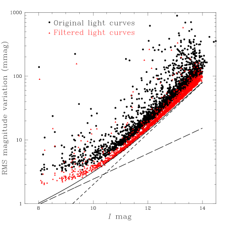
Figure 1: A typical example of the precision of the photometry we have obtained with our reduction pipeline and additional trend-filtering to remove systematic noise. The target field is Jan06_1 and light curves are comprised of 1713 data points. The solid circles are the original light curves produced by the pipeline; the hollow triangles show the improvement in the precision with the trend-filtering. The solid line shows the theoretical Poisson noise limits from the sky flux (short dashed line) and stellar flux (long dashed line).

3 Selection of variable candidates

Three methods were used to extract the variable light curves from the full data set: (i) visual inspection of the filtered light curves down to 13^th magnitude, (ii) implementation of a box-search algorithm on all filtered light curves (down to 14^th magnitude), and (iii) implementation of the Stetson Variability Index on the entire set of filtered and unfiltered light curves. The first two methods formed part of the search for transiting extrasolar planets, the main science driver of this project (Hidas et al., 2005). The third was implemented to improve the completeness of the catalogue.

3.1 Visual inspection

As a first pass, all light curves down to 13^th magnitude are visually inspected. This has the advantage of being reasonably immune to the effects of systematic variability in the light curves, since the brain can be quickly trained to filter out similar signals appearing in multiple light curves. However, it becomes less useful for light curves fainter than 13^th magnitude due to the increased shot noise; it can also fail for brighter stars where the variable signal is of low significance, and will not be evident until the light curve is phased with the correct period. Importantly, this method is not successful for the detection of variable light curves with periods greater than $\sim$5 d. In these cases, the light curve for each night appears essentially flat, especially to someone specifically searching for transit events on the order of a few hours. Also, visual inspection has the potential to miss light curves that exhibit only single or partial events on a single pass through.

3.2 Transit detection algorithm

The light curves are subsequently processed with a transit detection algorithm (Aigrain & Irwin, 2004) which searches for box-shaped transit events within specified transit duration and period windows. For each light curve, the algorithm determines the combination of epoch, transit duration and period within a specified range that returns the highest signal-to-noise (S/N) ratio. Subsequently, light curves with a S/N greater than some cut-off (typically $>$8.0, although this value varied with the degree to which each field was affected by systematics) when folded at the these parameters are visually inspected in both raw and folded formats. We have chosen the transit duration and period windows for maximum efficiency in the extrasolar planet transit search, using windows of 0.04–0.25 d and 1.0–5.0 d respectively. The algorithm will detect the variable light curves with parameters that fall within these windows: both the shallow transit events that are flagged as potential transiting planet candidates and the deeper events produced by detached eclipsing binary systems. Additionally, it returns many variable light curves which can be approximated to some extent by a box-shaped model lying within the required period range, including: grazing eclipsing binaries exhibiting V-shaped transits; continuously varying light curves that give a significant result when folded to an optimum period; and variable light curves with periods outside the specified window but where an integer number of periods is located within the window. It also has the additional advantage of detecting those light curves with only single or partial events and providing a potential period. However, it is not useful for detecting variable light curves with periods much shorter ($<$0.5 d) or much longer ($>$10 d) than the specified period window.

3.3 Stetson Variability Index

Neither of the preceding methods will rigorously detect the longest period variables in our light curves. In order to increase the completeness of this variable star catalogue it was essential to correct this bias. An additional method of detecting variability in light curves is the Stetson Variability Index (Stetson, 1996), a measure of the correlated signal in a light curve.

Using the notation of Stetson (1996), the index $J$ is given by

$$J=\frac{\sum_{k=1}^{n}w_{k}{\rm sgn}(P_{k})\sqrt{|P_{k}|}}{\sum_{k=1}^{n}w_{k}}$$ (2)

where $n$ pairs of observations have been defined. For the $k$th pair, with a weighting of $w_{k}$, the magnitude residuals are $\delta_{i(k)}$ and $\delta_{j(k)}$, where $i$ and $j$ are the observations forming the pair. We can therefore define the product of the magnitude residuals as $P_{k}=\delta_{i(k)}\delta_{j(k)}$, or $P_{k}=\delta_{i(k)}^{2}-1$ for single observations (where $i=j$). The term ${\rm sgn}(P_{k})$ is the sign (positive or negative) of $P_{k}$. We have calculated the magnitude residuals in the same manner as Stetson (1996), scaling by the individual observational errors and correcting for the statistical bias to the mean, giving

$$\delta=\sqrt{\frac{n}{n-1}}\left(\frac{\upsilon-\bar{\upsilon}}{\sigma_{\upsilon}}\right)$$ (3)

where $\upsilon$ is the measured magnitude of the observation, $\bar{\upsilon}$ is the mean magnitude over all observations, and $\sigma_{\upsilon}$ is the individual error on the observed magnitude. To form the pairs of observations we chose a timescale of 10 minutes; all observations that lie within 10 minutes of each other are paired. All pairs with $i\neq j$ are assigned a weight of 1.0, and those with $i=j$ a weight of 0.1. We found the best results in terms of detecting longer period variables ($>$ 1 d) when the data were binned on a similar timescale of $\sim$10 minutes, although this was at the cost of lowering the detection of the very shortest period variables. The solid squares in Figure 2 show a typical distribution of this variability index for a single field, in this case the Dec06 field as shown in Figure 1, prior to the trend-filtering stage.

One problem we encountered was the tendency for our implementation of the trend-filtering algorithm to suppress or entirely remove the night-to-night magnitude jumps present in the long-period variable light curves, resulting in a smaller than expected variability index. This was solved by running the variability index on both the filtered light curves to detect the shorter period variables and the unfiltered light curves to detect the longer period variables. The caveat to this is that long period trends in the systematic signals in the data, for instance signals correlated with moon phase, are not removed from the long period light curves. In an effort to overcome this, we have removed those long period light curves where multiple light curves in the same field demonstrate the same morphology and are described well by the same period and epoch. In the future we plan to resolve this problem by replacing the trend-filtering algorithm with an implementation of SYSREM (Tamuz, Mazeh & Zucker, 2005). Preliminary tests indicate this will not affect the longer period variable light curves in the same manner. The hollow triangles in Figure 2 show the distribution of the variability index after trend-filtering. For the unfiltered light curves, we set a cut-off of $J=1.0$, and for the filtered light curves we set $J=0.4$. We found these limits recovered 90–97% of the variables previously identified by visual inspection and the box-search algorithm, as well as over 150 long-period variables that had previously been undetected. The variables that were not recovered were generally the shallower longer period eclipsing binary light curves where the occasional small excursion from the mean magnitude was not sufficient to increase the variability index above the cut-off. Also missing were the shortest period variables with periods less than 1 hr, where the timescales for pairing and binning of 10 minutes were long enough to reduce the effectiveness of the variability index as a true measure of variability.

Figure 2: The Stetson Variability Index $J$ as a function of magnitude for the Dec06 field. The solid circles are the original light curves, and the hollow triangles are the filtered light curves. During the variable selection process unfiltered light curves with $J>1.0$ (the dotted line) and filtered light curves with $J>0.4$ (the dashed line) were flagged.

4 The light curve catalogue of variable stars

Using these methods, we find a total of 850 variable light curves in our data set. These have been analysed in a similar iterative fashion to Derekas et al. (2007) as follows. Initial periods have been determined with either the transit detection algorithm (for eclipsing light curves) or $\chi^{2}$ fitting of sine waves using discrete Fourier transforms (for continuously varying light curves). Each of the resulting phased curves was then visually inspected to assign a type of variability, and also to confirm that the automatically determined period was not half or an integer multiple of the real period, a common occurrence for light curves of eclipsing binaries. A visual inspection of every phase diagram was usually sufficient to show whether the determined period was an alias or was slightly inaccurate. In the case of an alias, we multiplied the initial period by different constants (in most cases by 2) until the shape of the curve was consistent with that of an eclipsing binary. For the long period variables, the observing baseline was typically insufficient to determine if the variability was periodic; in these cases the period and epoch are not supplied in the catalogue.

We next used the string-length method (Lafler & Kinman 1965; Clarke 2002) to improve the period determination (see also Derekas et al. 2007 for further details). We applied the method for 500 periods within $\pm 1$% of the best initial period guess. The typical period improvement resulted in a change in the 3rd-4th decimal place, consistent with the limited frequency resolution of the data (which scales with 1/T_obs, where T_obs is the time-span of the observations).

During the individual inspection of the phase diagrams, we made a visual classification of all 850 variables. Based on the light curve shapes alone, phased with the final adopted periods, we placed each star into one of the following categories: Algol-type (EA), $\beta$ Lyrae-type (EB), W Ursae Majoris-type (EW), RR Lyrae stars (RRL), Cepheids (DCEP), long period variables with periods $>10$ d (LPV), and pulsating variables with periods $<10$ d (including $\delta$ Scuti and other multiply periodic variables, referred to as PUL). We follow the convention of using a colon to indicate a loose classification (for example, EB:). In several cases we used the “spotted variable” type, which refers to singly periodic variables with periods of several days, light curve amplitudes of a few hundredths of a magnitude and light curve shapes characteristic of known rotationally variable active stars. These can be binaries or single stars, and have multi-periodic light variations on time scales of years and decades (see for example Oláh et al. 2000). We note that for sinusoidal light curve shapes, it is difficult to differentiate between the EW, PUL and spotted variable classifications by eye. Where there is an ambiguity between several classifications they are listed as, for example, EW/PUL. If there are two types of variability present they are listed as, for example, EA+PUL. If there is additional information it is given as, for example, RRL-Blazhko.

Figure 3: The variability amplitude detection limits for this catalogue. The mean $I$-band magnitude and the variability amplitude are plotted for the entire data set of variable light curves.

The detection limits of the catalogue are shown in Figure 3, with the mean $I$-band magnitude and variability amplitude plotted for all 850 variable light curves. For the detached eclipsing binaries the amplitude was the best-fitting transit depth as recorded by the box-search algorithm; for the continuously varying light curves we have used the amplitude from the sinusoid-fitting. For the multi-periodic light curves this will represent an approximate amplitude of the dominant frequency. As discussed in Section 2.2, due to dilution of the signal in crowded photometry apertures, the variability amplitudes presented here are lower limits on the true amplitudes. From Figure 3 it is apparent that around $I\approx 12$ mag we lose sensitivity to the lowest amplitude variables (such as the multi-periodic $\delta$ Scuti stars or pulsating red giants), while for $I>13$ mag only the highest amplitude pulsators (RR Lyrae stars) and eclipsing binaries remain.

The last step in the variable star analysis was cross-correlation with existing databases to supplement the catalogue with as much additional information as possible. Namely, we queried the most recent update of the General Catalogue of Variable Stars (GCVS, Samus et al. 2007), including the New Suspected Variables catalogue, to identify already known variable stars. In addition, we checked the ASAS-3 database of southern variables (Pojmanski 2002). This revealed that 191 out of 850 variables are positionally coincident with previously published variable stars, leaving the total number of our new discoveries at 659. This corresponds to 78%, which is a lower fraction than, for instance, the 90% new discoveries found by Hartman et al. (2004) in the HATNet observations of the Kepler field. However, it is still surprisingly large, given the fact that the ASAS-3 project had previously observed each of our fields, whereas the Kepler field had not been targeted with variability surveys prior to the Hartman et al. study. We also performed a cross-correlation with the 2MASS Point Source Catalog (Skrutskie et al. 2006) to provide $JHK$ magnitudes. Where multiple 2MASS sources are present within the APT photometry aperture, the source closest to the centre of the photometry aperture that is brighter than $J\sim 15$ mag is selected. Finally the catalogue was cross-correlated with the ROSAT X-Ray Source Catalog (Voges et al., 1999, 2000) to determine which sources, if any, might be active stars with hot coronae.

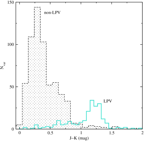
Figure 4: A comparison of the colour histograms for LPV and non-LPV variables.

A histogram of the $J-K$ colour indices (Figure 4) for the LPV and non-LPV variables (the latter including all eclipsing binaries and classical pulsators) demonstrates the expected dichotomy, with LPVs mostly having $J-K>0.6$ mag, i.e. being red giant stars. A few LPVs have bluer colours, which might indicate early-type stars with longer periods unrelated to red giant pulsations (e.g. ellipsoidal variability in binaries, rotational modulation due to starspots), or mismatches with the 2MASS catalogue. Conversely, most of the non-LPVs have $J-K<0.7$ mag, corresponding to spectral types A–K. The few redder non-LPVs are all located at lower galactic latitudes, suggesting strong interstellar reddening in their cases.

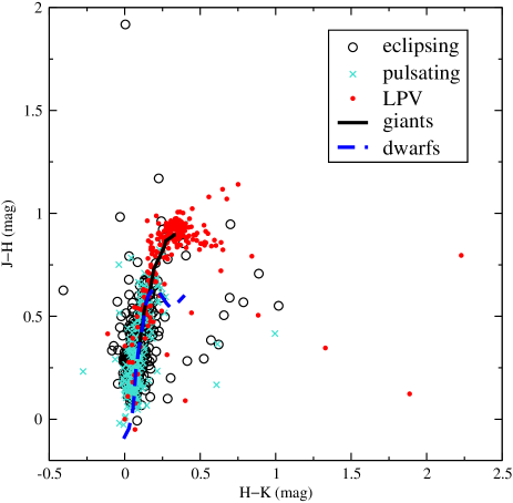
Figure 5: The $J-H$ vs. $H-K$ colour-colour diagram with the three broad categories and the stellar loci taken from Bessell & Brett (1988).

We also tested the consistency between the assigned variability types and their expected stellar types via the $J-H$ vs. $H-K$ colour-colour diagram. Using the intrinsic stellar loci determined for dwarfs and giants by Bessell & Brett (1988) and transformed into the 2MASS system (Carpenter 2001), we plot the locations of stars in three broad categories (eclipsing, pulsating, LPV) in Figure 5. Here we find a good agreement: almost all LPVs follow the intrinsic location of red giant stars, even showing hints of the separate carbon-rich LPV sequence for $J-K>1.0$ mag and $H-K>0.4$ mag. There are several outliers towards both bluer and redder $H-K$ colours, almost exclusively eclipsing binaries, where we may suspect high reddening, mismatches with the 2MASS catalogue, composite colours of stars blended in the 2MASS catalogue, which has a spatial resolution of 1 arcsec pixel^-1, or large photometric errors in the 2MASS magnitudes.

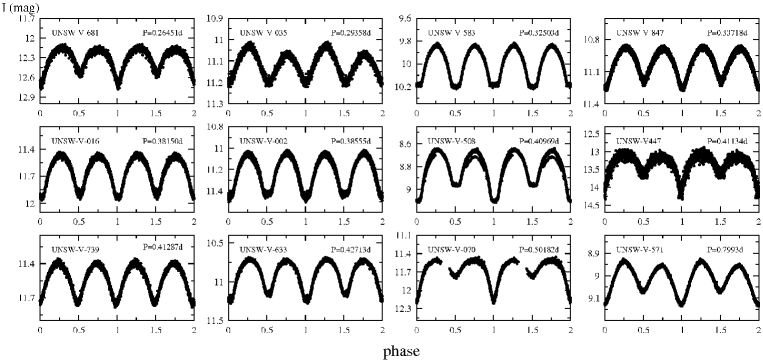
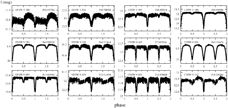
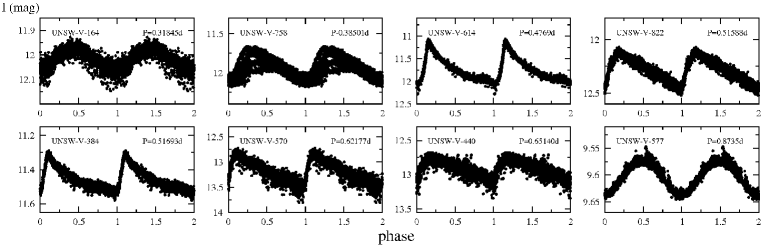
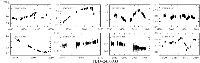
Figure 6: Sample light curves for contact eclipsing binaries (top three rows), detached eclipsing binaries (next three rows), RR Lyrae stars (next two rows) and LPV (bottom two rows). These light curves have not been processed with the trend-filtering algorithm.

As an indication of the quality of the light curves in this catalogue, we plot a representative sample of eclipsing binaries, pulsating variables and LPVs (Figure 6). All data are publicly available at the University of New South Wales Virtual Observatory facility (see Section 6). Table 2 contains an extract of the complete summary table available in the electronic version of this paper. For each star the ID, J2000 coordinates, galactic coordinates, 2MASS $JHK$ magnitudes, mean $I$-band magnitude, $I$-band amplitude, period, epoch of minimum light, previous identifier where appropriate and classification in this catalogue are shown.

Table 2: Extract from the complete catalogue included in the electronic version of this paper. See text for an explanation of the columns.

ID	RA	Dec	$l$∘	$b$∘	$J$	$H$	$K$	$I$	$A$	Period	Epoch	Alternate ID	Type
	(J2000.0)	(J2000.0)			(mag)	(mag)	(mag)	(mag)	(mag)	(d)	HJD-2450000.0
UNSW-V-001	04:52:56.7	$-$29:48:14.3	231.0476	$-$37.4715	8.258	7.805	7.650	8.66	0.012	-	-		LPV
UNSW-V-002	04:53:38.1	$-$29:06:38.0	230.2417	$-$37.1672	11.228	10.933	10.821	11.23	0.200	0.38555	3289.1020	ASAS 045338-2906.6	EW
UNSW-V-003	04:53:48.2	$-$29:53:49.2	231.2140	$-$37.3108	12.475	12.078	11.969	12.71	0.026	0.69570	3289.0900		EA
UNSW-V-004	04:54:43.8	$-$29:34:07.0	230.8696	$-$37.0407	12.388	12.111	12.083	12.46	0.018	-	-		LPV
UNSW-V-005	04:57:28.8	$-$29:09:48.3	230.5523	$-$36.3636	8.540	8.235	8.160	8.75	0.005	3.2684	3289.1200		EB
UNSW-V-006	04:57:45.4	$-$30:14:05.8	231.8658	$-$36.5529	9.342	9.162	9.109	9.38	0.003	-	-		LPV
UNSW-V-007	04:58:03.5	$-$29:55:59.1	231.5185	$-$36.4208	10.068	9.823	9.745	10.21	0.128	3.0683	3324.2200	ASAS 045804-2956.0	EA
UNSW-V-008	04:58:18.2	$-$29:04:54.7	230.5073	$-$36.1695	13.720	13.279	13.238	13.73	0.050	0.31036	3288.9700		EW
UNSW-V-009	04:50:06.9	$-$30:39:50.7	231.9448	$-$38.2536	13.548	13.424	13.386	13.69	0.139	1.0641	3351.9800		EA
UNSW-V-010	04:50:18.7	$-$30:21:29.1	231.5754	$-$38.1480	11.697	11.139	10.976	12.31	0.032	1.9175	3290.4200		PUL

5 Discussion

An extensive collection of variable stars always leads to some unexpected results: in the course of analysing transit candidates, the University of New South Wales Extrasolar Planet Search has identified a low-mass K7 Ve detached eclipsing binary (M${}_{\rm tot}=1.04\pm 0.06$ M_⊙, Young et al. 2006) and the first high-amplitude $\delta$ Scuti star in an eclipsing binary system (Christiansen et al. 2007). While these alone are interesting, the full breadth of the data is much more extensive. Below we discuss several possible applications, making no attempt at completeness.

5.1 Close eclipsing binaries with extreme properties

Contact binaries (or W UMa-type eclipsing variables) are among the most common types of variable stars, occurring at a rate of roughly 1 in every 500 FGK dwarfs (Rucinski 2006), which explains their large occurrence rate in variable star catalogues (e.g. 218 out of 850 in this catalogue). One intriguing problem related to these stars is that of binary mergers. When the total angular momentum of a binary system is at a certain critical (minimum) value, a secular tidal instability occurs which eventually forces the stars to merge into a single, rapidly rotating object (Arbutina 2007 and references therein). In the case of contact binaries, the instability occurs at a minimum mass-ratio of $q_{\rm min}\sim 0.071-0.076$ (Rasio 1995, Li & Zhang 2006), which has been the explanation for the very few contact systems with $q<0.1$ (see Arbutina 2007 for the updated lists of ten contact systems in the range of 0.065-0.13). The exact limit depends on assumptions on the stellar structure and dynamical stability (Li & Zhang 2006). Since it is likely that at least a fraction of blue straggler stars in star clusters formed via binary mergers (Mapelli et al. 2004), there is an exciting opportunity to constrain binary merger theories by increasing the number of known contact binaries with extremely low mass-ratios, and probing the limits of the observed $q_{\rm min}$.

Figure 7: Possible candidates for low mass-ratio contact binaries.

Examining the published light curves of the lowest mass-ratio systems (e.g. AW UMa: Pribulla et al. 1999; V870 Ara: Szalai et al. 2007), a single flat-bottomed minimum is always present, which corresponds to the full eclipse of the much smaller component that occurs within a certain range of inclinations. In our sample we find about five binaries with very similar periods (0.3–0.4 d) and light curve shapes (three are shown Figure 7), which might therefore be low mass-ratio systems deserving further attention. This could include obtaining and modelling multi-colour light curves in several bands (see, e.g., Qian et al. 2005).

Similarly to the mass-ratio, contact binary periods also have a very well-defined cut-off, which occurs at $P\approx 0.215-0.22$ d, just 0.05 d shorter than the maximum of the volume-corrected period distribution (Rucinski 2007). Stepien (2006) attempted to explain the period cut-off via the magnetic-wind driven angular momentum loss, the rate of which shows a progressive decay with the shortening of the period so that the period evolution takes progressively longer time. The period cut-off would then be due to a finite age of the binary population of several Gyr. Using the ASAS sample of binaries, Rucinski (2007) concluded that while no evidence exists for angular momentum evolution, the drop in numbers towards the cut-off still suffers from small number statistics and the cut-off itself remains unexplained. Hence, improving the statistics at the short-period end of contact binaries is important, where high-cadence transit search programs could play an important role. In our sample, there are four contact binaries out of 218 in the range of $P=0.246-0.250$ d, which fall on the short-period end of the distribution but do not improve the statistics near the cut-off (the present record holder in the Galactic field has a period of 0.2178 d; Rucinski 2007).

It is also possible to use the periods and light curve morphologies to identify close eclipsing binaries that are potentially composed of low-mass components. Identifying low-mass stars in eclipsing binaries is extremely important for accurately deriving the fundamental stellar parameters of mass and radius that are crucial for constraining low-mass stellar formation and evolution models. Following the method of Weldrake et al. (2007), we select those contact binaries with periods $<0.25$ d, and Algol-type detached eclipsing binaries with no obvious out-of-eclipse variations and periods $<1.6$ d as good candidates for low-mass eclipsing binary systems. We find four contact binaries (the same four located near the period cut-off) and 31 detached binaries matching these criteria, listed in Table 3. There are quite a few bright ($I>12$) objects in this list which would make excellent targets for spectroscopic follow up.

Table 3: Eclipsing binary systems potentially composed of low-mass components.

ID	RA(J2000.0)	Dec(J2000.0)	$I$ (mag)	P (d)
Contact eclipsing binaries
UNSW-V-077	09 30 05.4	$-$14 02 17.9	12.64	0.2480
UNSW-V-219	16 55 48.1	$-$60 19 08.7	13.50	0.2456
UNSW-V-659	21 07 03.6	$-$65 56 42.0	11.08	0.2472
UNSW-V-662	21 10 21.6	$-$66 54 53.3	12.37	0.2492
Detached eclipsing binaries
UNSW-V-003	04 53 48.2	$-$29 53 49.2	12.71	0.6956
UNSW-V-090	11 56 40.6	$-$35 43 43.8	12.53	1.1870
UNSW-V-097	11 59 53.9	$-$36 13 26.1	12.18	0.9025
UNSW-V-143	16 57 00.6	$-$60 29 51.9	12.17	0.8117
UNSW-V-156	17 00 06.2	$-$60 17 02.4	13.43	1.5618
UNSW-V-192	17 09 18.1	$-$60 01 43.5	13.45	1.4877
UNSW-V-198	17 10 18.2	$-$59 46 08.9	13.20	1.2275
UNSW-V-205	17 13 55.3	$-$60 12 15.3	11.83	0.9610
UNSW-V-301	17 16 37.3	$-$58 09 40.4	11.04	1.4828
UNSW-V-312	00 00 06.0	$-$59 44 48.3	13.63	1.0574
UNSW-V-353	04 04 51.2	$-$24 11 30.4	13.73	0.7065
UNSW-V-379	09 22 49.7	$-$25 12 40.8	13.35	0.4975
UNSW-V-386	09 14 14.5	$-$24 53 31.6	11.43	1.2956
UNSW-V-410	09 13 47.8	$-$22 48 23.5	13.07	0.9690
UNSW-V-472	13 08 49.2	$-$44 47 55.2	12.46	0.5484
UNSW-V-527	14 45 10.0	$-$39 25 47.3	10.99	1.363
UNSW-V-528	14 45 19.4	$-$38 08 48.0	11.26	1.211
UNSW-V-536	14 47 27.5	$-$38 31 36.7	11.56	0.2303
UNSW-V-540	14 49 09.1	$-$38 38 10.1	12.92	0.5216
UNSW-V-598	18 21 14.1	$-$64 30 03.1	11.77	0.8492
UNSW-V-617	18 38 00.5	$-$65 06 07.7	10.66	1.5092
UNSW-V-621	18 11 49.9	$-$67 06 13.8	13.76	1.0194
UNSW-V-624	18 18 48.4	$-$67 27 54.1	12.76	1.482
UNSW-V-644	18 34 50.6	$-$67 24 09.9	12.96	1.4238
UNSW-V-683	20 58 55.7	$-$67 02 12.8	13.21	1.0740
UNSW-V-696	21 08 04.4	$-$68 57 53.1	11.55	0.9428
UNSW-V-706	20 58 35.9	$-$69 04 01.4	12.03	1.025
UNSW-V-722	23 25 23.1	$-$70 01 48.5	12.20	1.3523
UNSW-V-740	08 04 02.0	$-$66 28 02.6	13.63	1.2634
UNSW-V-746	08 08 27.0	$-$68 19 07.5	12.68	1.0324
UNSW-V-846	15 03 44.5	$-$68 40 02.6	12.13	1.5804

5.2 Pre-main-sequence eclipsing binaries

Detached eclipsing binaries provide one of the most accurate (largely model-independent) sources of fundamental stellar parameters, notably masses and radii. These can be used to put the strongest constraints on stellar evolutionary models, which in turn can improve our understanding of the formation and evolution of individual stellar populations. On the pre-main-sequence, the calibration of stellar parameters is presently extremely scarce below 1 M_⊙ where only six eclipsing binaries are known, all located in the Taurus-Orion region (Irwin et al. 2007). Comparison of these systems to different stellar models have indicated difficulties in fitting both components of the binaries simultaneously, which shows our current models of low-mass stars are seriously challenged by the known systems (see also Aigrain et al. (2007)).

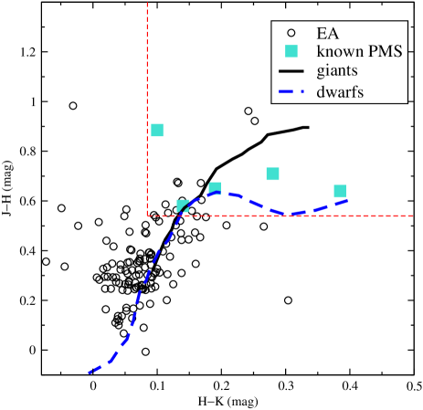
Figure 8: Detached binaries and the location of five known pre-main-sequence eclipsing systems (data taken from Stassun et al. 2004, Covino et al. 2004, Hebb et al. 2006, Stassun, Mathieu & Valenti 2007 and Irwin et al. 2007).

Table 4: Candidate PMS detached binaries

ID	RA(J2000.0)	Dec(J2000.0)	$I$ (mag)	P (d)
UNSW-V-097	11 59 53.9	$-$36 13 26.1	12.18	0.90251
UNSW-V-107	12 03 06.8	$-$35 37 47.5	12.40	6.23034
UNSW-V-299	17 16 10.8	$-$57 20 37.5	12.33	5.97542
UNSW-V-312	00 00 06.0	$-$59 44 48.3	13.63	1.05762
UNSW-V-491	13 12 31.5	$-$46 04 08.8	12.76	3.83246
UNSW-V-518	13 07 31.8	$-$45 12 42.0	12.59	2.75743
UNSW-V-617	18 38 00.5	$-$65 06 07.7	10.66	1.50906
UNSW-V-676	21 20 45.9	$-$66 22 18.5	13.50	3.28503
UNSW-V-722	23 25 23.1	$-$70 01 48.5	12.20	1.01274
UNSW-V-746	08 08 27.0	$-$68 19 07.5	12.68	1.03214

One possibility for identifying pre-main-sequence binaries is by using colour-colour diagrams, such as the one depicted in Figure 8. Here we plot the location of the detached binaries in our sample, using 2MASS $JHK$ magnitudes, the intrinsic stellar loci from Bessell & Brett (1988) and the position of five PMS binaries with published $JHK$ photometry (mostly from 2MASS). We use two dashed lines as boundaries for defining a PMS candidate: the vertical and horizontal lines are at $H-K=0.085$ mag and $J-H=0.54$ mag, respectively. In total we extract 17 Algol-type systems from our sample that have redder colours than the boundary lines (i.e. located around the known PMS systems in Figure 8). Investigation of higher spatial resolution archived images from the Digitized Sky Surveys (DSS) demonstrates that in six cases, the APT photometry aperture contains a single central 2MASS source. In four additional cases, the aperture contains a single bright source and up to half a dozen additional sources several magnitudes fainter, where the depth of the eclipse ($>0.5$ mag) precludes the fainter sources from producing binary signal.

These ten are listed in Table 4: some could be heavily reddened main-sequence stars, but since the majority of our fields are located above a Galactic altitude of 15^∘, there is the distinct possibility of genuine PMS binaries in the sample. There is also the possibility of composite colours of unresolved blends in the 2MASS catalogue. One method of confirmation would be obtaining high-resolution spectroscopy to look for PMS signatures, such as strong Li absorption (Irwin et al. 2007)

5.3 The Blazhko-effect in RR Lyrae stars

RR Lyrae stars are horizontal branch stars showing high-amplitude pulsations driven by the $\kappa$-mechanism, with typical periods of about 0.5 days. It is known that a large fraction of RR Lyrae stars (20–30% of the fundamental mode RRabs and 2% of the first-overtone RRcs, Kovács 2001) exhibit periodic amplitude and/or phase modulations, the so-called Blazhko-effect, which is one the greatest mysteries in classical pulsating star research. Currently, two classes of models are usually put forward as possible explanations, both assuming the presence of non-radial oscillations (note, that RR Lyrae stars have long been considered as the prototypes of purely radially pulsating stars): the resonance models, in which resonance effects excite non-radial modes in addition to the main radial mode, and the magnetic models, which are essentially oblique rotating pulsator models (see Kolenberg et al. 2006 and references for more details). Recently, Stothers (2006) published a new explanation, in which turbulent convection inside the hydrogen and helium ionization zones becomes cyclically weakened and strengthened owing to the presence of a transient magnetic field that is generated by some kind of a dynamo mechanism.

Table 5: RR Lyrae stars with detected Blazhko-effect and double-mode pulsation.

ID	RA(J2000.0)	Dec(J2000.0)	$I$ (mag)	P (d)
Blazhko-effect
UNSW-V-101	12 00 49.6	$-$36 11 59.2	14.26	0.6264
UNSW-V-203	17 12 35.0	$-$60 29 32.1	11.99	0.4933
UNSW-V-384	09 24 25.5	$-$24 05 03.4	11.45	0.5169
UNSW-V-442	12 50 44.3	$-$44 41 20.3	13.08	0.5853
UNSW-V-614	18 34 41.2	$-$65 27 08.1	11.74	0.4769
UNSW-V-773	14 40 40.8	$-$68 23 16.8	11.03	0.5518
Double-mode
UNSW-V-358	09 16 04.3	-23 36 08.0	13.49	0.3602
				0.4840
UNSW-V-532	14 46 35.8	-39 33 31.7	12.86	0.6540
				0.5012
UNSW-V-577	14 52 42.1	-41 41 55.3	9.60	0.8735
				0.6682
UNSW-V-758	08 16 09.3	-66 44 46.3	11.94	0.3850
				0.5170
UNSW-V-810	14 50 13.3	-69 45 18.5	11.70	0.7372
				1.0576

With a variety of competing models, theory is in desperate need for further empirical constraints, most notably ones that are capable of detecting non-radial oscillations and/or magnetic fields, for example high-resolution spectroscopy. Hence, the discovery of bright to moderately faint RR Lyrae stars with well-expressed Blazhko-effect could be of great interest. In our sample we find six RR Lyrae stars out of 52, listed in Table 5, that demonstrate the Blazhko-effect. Four were previously known variables, and two are new discoveries. The Blazhko-period of modulation for RR Lyrae stars typically ranges from tens to hundreds of days (see, for example, fig. 4 of Szczygiel & Fabrycky (2007)), although they can be as short as a few days (Jurcsik et al., 2006). Due to the comparable baseline of our observations, we could not determine the Blazhko-period for any of the stars, but the four objects brighter than $I\sim 12$ mag, one of which is a new discovery, are good candidates for further studies. We also find five double-mode RR Lyrae stars, for which the period ratios suggest the well-known mixture of fundamental+first radial overtone pulsation. Three of these are new discoveries, with two previous published in the ASAS-3 catalogue, thus raising the total number of field double-mode RR Lyrae stars known in the Galaxy to 30; see Szczygiel & Fabrycky (2007).

6 Online access to light curves

All APT images from 2002 July until present day, including those used in the creation of this catalogue, are stored in a publicly available archive. This archive can be accessed using a web browser and the conventional web interface located at:

http://astro.ac3.edu.au

Alternatively, the archive can be accessed via the Simple Image Access Protocol (SIAP) (Tody & Plante 2004) as defined by the International Virtual Observatory Alliance (IVOA). The SIAP defines a standard for retrieving images from a repository using simple URL-based queries. For example, a request made to the following URL will return a list of APT images that intersect with the 1 degree square region centred on (75,-30) with RA and Dec expressed in decimal degrees:

http://astro.ac3.edu.au/unsw/siap?POS=75,-30&SIZE=1&TEL=APT

The POS parameter is mandatory and defines the centre of the search region. The SIZE parameter is optional (default is SIZE=1) and determines the size of the search region. The TEL parameter distinguishes between images from different telescopes, and is specific to the UNSW implementation of the SIAP service.

The list of images returned by the SIAP query is in VOTable format (Ochsenbein et al. 2004). Each item in the list contains a set of attributes describing a particular image that satisfies the search criteria. Also included is a URL which can be used to download the associated image.

The catalogue of light curves discussed in this paper is available from the UNSW archive via the Simple Spectral Access Protocol (SSAP) (Tody et al 2007). The SSAP is an IVOA standard for accessing archives of one dimensional spectra, including time series data such as light curves. The format of an SSAP query is very similar to the format of an SIAP query. For example, the query specified in the following URL will search for light curves of stars within a circle of diameter 1 degree centred at the point (75,-30).

http://astro.ac3.edu.au/unsw/ssap?REQUEST=queryData&POS=75,-30&SIZE=1

The REQUEST parameter is the only mandatory parameter. The optional parameters include POS, SIZE, BAND and TIME, which are used to constrain the search by region (degrees), bandpass (metres) and time of observation (ISO 8601).

The list of light curves returned by the SSAP query is in VOTable format, and each item in the list contains a set of metadata describing a particular light curve, including a URL for downloading the data. The light curve data itself is also presented in VOTable format and follows the structure of the Spectrum Data Model (McDowell 2007). Consequently, these light curve VOTables may be examined with any VO-compliant tool, such as TOPCAT (Taylor 2005).

7 Summary

We have presented a catalogue of 850 variable stars, compiled from 32 months of observations obtained for the University of New South Wales Extrasolar Planet Search. Of these stars, 659 are new discoveries that have not been previously reported in the GCVS, NSV or ASAS-3 catalogues. This catalogue of well-sampled high precision light curves, each spanning 1–4 months, has significant potential for astrophysically interesting data mining. We have nominated several possibilities, including eclipsing binary systems with low mass ratios, low-mass components or pre-main sequence components, and RR Lyrae stars demonstrating the curious Blazhko-effect. The data have been made publicly available on the University of New South Wales VO server in a standard format for retrieval and for analysis with standard VO tools.

Appendix A Cross-identifications with the GCVS, ASAS and ROSAT catalogues

The positions of the stars in this catalogue were correlated with the General Catalog of Variable Stars (GCVS) and All Sky Automated Survey (ASAS) variable star catalogues, using the Vizier online database (Ochsenbein et al., 2000). The photometry aperture used in our data reduction pipeline has a radius of 28.2^′′, and so a simple cone search with a radius of 30^′′ was performed. The results of the correlation are shown in Table 6. 191 of the 850 stars presented in this catalogue are positionally coincident with previously published variable stars. The columns in the table are the UNSW identifier from this catalogue, the right ascension and declination (J2000.0), the mean $I$-band magnitude, $I$-band amplitude of variation, period, epoch, the identifier from either the GCVS, NSV or ASAS catalogues, and our classification, which was found to be in good agreement with the published classification in more than 90% of the cases with a few exceptions, like V717 Ara (EB), which is listed as an RR Lyr in the GCVS or V500 Ara (EW), also RR Lyr in the GCVS. However, these are the classes with highly sinusoidal, i.e. indistinguishable light curve shapes, and it is therefore not surprising that single-filtered light curves are not enough in doubtful cases.

The positions were also correlated with x-ray sources in the ROSAT 1RXS (Voges et al., 1999, 2000) and 2RXP (ROSAT 2000) catalogues, similarly to Norton et al. (2007). The search was again performed through Vizier using a 30^′′ cone search, and the results are shown in Table 9. The columns are as for Table 61, although in this case the second identifier column contains the ROSAT source identifier. 22 of the 850 stars were found to be spatially coincident with ROSAT sources, although we note that since the majority have been classified as pulsating variables, which are not expected to be strong X-ray sources (Makarov 2003), it is doubtful how much of the coincidence is real.

Table 6: UNSW variable stars coincident with GCVS/ASAS records.

ID	RA	Dec	$I$	$A$	Period	Epoch	Alternate ID	Type
	(J2000.0)	(J2000.0)	(mag)	(mag)	(d)	HJD-2450000.0
UNSW-V-002	04 53 38.1	$-$29 06 38.0	11.23	0.200	0.38555	3289.1020	ASAS 045338-2906.6	EW
UNSW-V-007	04 58 03.5	$-$29 55 59.1	10.21	0.128	3.06827	3324.2200	ASAS 045804-2956.0	EA
UNSW-V-011	05 00 55.6	$-$30 07 54.1	12.06	0.127	0.84183	3291.1200	ASAS 050056-3007.9	EW
UNSW-V-013	05 02 46.6	$-$29 44 04.2	8.41	0.026	-	-	ASAS 050247-2944.1	LPV
UNSW-V-016	04 51 51.6	$-$29 34 22.4	11.65	0.209	0.38150	3289.3880	ASAS 045151-2934.3	EW
UNSW-V-018	04 42 00.0	$-$25 28 45.5	13.52	0.134	0.58747	3289.1000	ASAS 044200-2528.8	RRL
UNSW-V-019	04 42 16.3	$-$25 49 32.1	11.46	0.220	0.25489	3285.3350	ASAS 044216-2549.5	EW
UNSW-V-021	04 42 25.4	$-$26 17 31.3	11.52	0.087	0.45552	3285.2000	ASAS 044225-2617.5	EW
UNSW-V-026	04 48 00.9	$-$25 31 23.1	12.23	0.200	0.54883	3285.1700	ASAS 044801-2531.4	RRL
UNSW-V-035	09 03 32.6	$-$14 52 45.5	11.12	0.070	0.29358	3376.9850	ASAS 090333-1452.8	EW
UNSW-V-043	09 05 55.6	$-$14 51 23.4	10.90	0.069	0.56636	3377.1500	ASAS 090556-1451.4	EW
UNSW-V-046	09 07 07.5	$-$14 07 37.7	9.84	0.041	-	-	ASAS 090708-1407.7	LPV
UNSW-V-050	09 08 20.6	$-$13 35 43.2	11.14	0.068	15.44279	3389.0400	ASAS 090821-1335.8	EA
UNSW-V-055	08 59 54.2	$-$15 15 22.9	11.57	0.186	0.39362	3371.1350	ASAS 085954-1515.4	EW
UNSW-V-057	09 22 21.2	$-$13 38 50.4	12.50	0.188	0.53220	3377.9800	IV HYA/ASAS 092220-1338.8	RRL
UNSW-V-061	09 23 55.7	$-$14 20 22.1	8.65	0.026	35.06803	3393.0000	ASAS 092356-1420.4	LPV
UNSW-V-062	09 24 55.9	$-$13 11 58.2	12.92	0.180	0.61124	3382.1500	ASAS 092456-1312.0	RRL
UNSW-V-066	09 26 41.0	$-$13 45 06.5	9.66	0.239	0.44976	3377.2500	EZ HYA/ASAS 092641-1345.1	EW
UNSW-V-070	09 28 20.1	$-$12 50 51.2	11.70	0.248	0.50182	3377.0970	ASAS 092820-1250.9	EB
UNSW-V-071	09 28 28.7	$-$13 26 33.2	11.68	0.205	0.73146	3378.4340	ASAS 092829-1326.5	EB
UNSW-V-074	09 28 57.5	$-$13 07 12.4	8.16	0.029	45.49365	3402.0000	ASAS 092857-1307.2	LPV
UNSW-V-075	09 29 15.3	$-$14 05 57.2	12.27	0.263	0.33259	3377.2450	ASAS 092915-1405.9	EW
UNSW-V-081	09 20 17.4	$-$14 05 09.7	8.61	0.099	-	-	ASAS 092018-1405.1	LPV
UNSW-V-084	11 55 44.0	$-$36 26 19.8	11.78	0.134	0.53132	3415.1900	ASAS 115544-3626.3	EW
UNSW-V-086	11 56 12.9	$-$35 59 29.9	11.50	0.266	0.37801	3415.1180	V0576 CEN/ASAS 115613-3559.5	EW
UNSW-V-087	11 56 20.4	$-$35 28 45.5	11.39	0.141	0.29374	3415.3250	ASAS 115620-3528.8	EW
UNSW-V-090	11 56 40.6	$-$35 43 43.8	12.53	0.102	1.18713	3415.1300	V577 CEN	EA
UNSW-V-091	11 57 20.2	$-$36 40 23.3	13.52	0.133	0.58688	3422.9900	V0580 CEN	RRL
UNSW-V-092	11 57 57.2	$-$36 06 10.3	13.41	0.266	0.34622	3415.1670	V0581 CEN	EW
UNSW-V-097	11 59 53.9	$-$36 13 26.1	12.18	0.057	0.90251	3422.1700	NSV 05410	EA
UNSW-V-101	12 00 49.6	$-$36 11 59.2	14.26	0.170	0.62644	3423.0900	V0582 CEN	RRL
UNSW-V-105	12 02 27.6	$-$35 26 39.3	14.04	0.143	0.67441	3423.0800	EF HYA	RRL
UNSW-V-107	12 03 06.8	$-$35 37 47.5	12.40	0.078	6.23034	3415.0100	NSV 05437	EA
UNSW-V-115	11 53 52.2	$-$35 26 55.4	13.57	0.084	0.58367	3415.1200	DS HYA	RRL
UNSW-V-116	11 54 06.9	$-$35 14 54.8	11.22	0.082	3.30294	3423.1900	ASAS 115407-3514.9	EA
UNSW-V-122	11 56 27.7	$-$38 08 51.3	8.85	0.077	84.16663	-	ASAS 115628-3808.9	LPV
UNSW-V-131	12 01 25.6	$-$37 24 52.6	8.35	0.583	135.44203	-	V0583 CEN/ASAS 120125-3724.9	LPV
UNSW-V-132	12 02 19.3	$-$38 46 22.3	12.86	0.264	0.45906	3415.0900	V0584 CEN/ASAS 120219-3846.4	RRL
UNSW-V-137	12 06 53.6	$-$37 37 36.0	12.51	0.157	0.39816	3415.3260	ASAS 120654-3737.7	EW
UNSW-V-138	11 53 40.7	$-$38 22 00.5	10.55	0.063	0.82146	3423.5700	ASAS 115341-3822.1	EW
UNSW-V-140	16 56 35.0	$-$59 04 41.2	10.44	0.580	184.16278	-	CG ARA	LPV
UNSW-V-143	16 57 00.6	$-$60 29 51.9	12.17	0.020	0.81166	3510.1600	V0805 ARA	EA
UNSW-V-144	16 57 15.2	$-$60 08 05.3	12.71	0.224	0.92708	3499.5400	V0705 ARA	EW
UNSW-V-145	16 57 50.6	$-$59 07 20.0	12.60	0.187	0.57442	3509.1100	V0414 ARA	RRL
UNSW-V-147	16 57 43.8	$-$60 41 16.4	9.33	0.086	1.20159	3499.8030	ASAS 165744-6041.3	EW
UNSW-V-154	16 59 07.2	$-$60 05 25.4	8.55	0.903	174.95479	-	LS ARA/ASAS 165907-6005.4	LPV
UNSW-V-171	17 02 35.4	$-$59 30 48.7	9.84	0.302	118.49562	-	V0810 ARA	LPV
UNSW-V-178	16 54 36.1	$-$60 09 04.8	10.68	0.375	-	-	V0696 ARA	LPV
UNSW-V-184	17 05 59.3	$-$59 40 34.1	12.63	0.033	0.51838	3499.1100	V0464 ARA	RRL
UNSW-V-186	17 06 48.2	$-$59 03 20.0	8.68	0.864	152.13318	-	CH ARA/ASAS 170648-5903.3	LPV
UNSW-V-187	17 07 32.4	$-$60 58 45.6	11.47	0.117	2.32845	3504.1400	ASAS 170732-6058.8	EA
UNSW-V-194	17 09 43.0	$-$60 31 14.9	12.27	0.170	0.35894	3499.2330	ASAS 170944-6031.2	EW
UNSW-V-195	17 10 07.8	$-$60 39 45.7	10.51	0.134	2.52195	3499.2000	V0617 ARA/ASAS 171008-6039.8	CEP
UNSW-V-198	17 10 18.2	$-$59 46 08.9	13.20	0.072	1.22754	3555.2400	V0485 ARA	EA
UNSW-V-199	17 11 16.1	$-$60 20 42.8	8.69	0.637	184.16278	-	CN ARA	LPV
UNSW-V-200	17 11 32.5	$-$60 14 35.9	9.46	0.273	152.13318	-	NSV 08245	LPV
UNSW-V-203	17 12 35.0	$-$60 29 32.1	11.99	0.045	0.49332	3504.2800	CS ARA	RRL
UNSW-V-207	17 13 52.6	$-$59 05 16.1	9.56	0.137	75.56063	-	V0733 ARA/ASAS 171352-5905.2	LPV
UNSW-V-214	17 15 58.6	$-$60 04 06.2	11.25	0.129	0.40006	3499.1600	ASAS 171559-6004.1	EW
UNSW-V-215	17 16 19.3	$-$59 55 07.2	12.77	0.072	0.77541	3504.2500	DG ARA	RRL
UNSW-V-217	17 16 35.5	$-$60 21 01.4	11.65	0.204	0.36364	3499.1060	V0791 ARA/ASAS 171636-6021.1	EW
UNSW-V-218	17 17 40.0	$-$60 31 19.1	11.77	0.066	0.59981	3499.1400	MT ARA	EB
UNSW-V-229	17 01 00.5	$-$58 35 18.1	12.12	0.066	1.28635	3504.2500	V717 ARA	EW
UNSW-V-231	17 01 23.8	$-$58 16 46.1	12.90	0.036	0.58292	3504.1000	V0441 ARA	RRL
UNSW-V-232	17 01 33.8	$-$58 18 35.1	13.47	0.047	2.04759	3558.1000	V0442 ARA	EA
UNSW-V-233	17 01 49.3	$-$57 59 33.5	10.25	0.712	166.85367	-	V0779 ARA	LPV
UNSW-V-238	17 02 59.7	$-$57 06 42.8	9.49	0.080	0.98892	3510.2800	V0722 ARA	EA
UNSW-V-248	16 57 56.7	$-$57 52 46.4	10.94	0.471	-	-	V0776 ARA	LPV
UNSW-V-252	17 06 37.5	$-$58 07 40.2	11.02	0.124	0.89702	3504.2500	ASAS 170637-5807.7	EW
UNSW-V-254	17 06 33.9	$-$57 42 51.4	8.71	0.163	129.34859	-	NSV 08172/ASAS 170634-5742.9	LPV
UNSW-V-255	17 06 46.4	$-$58 31 15.2	12.05	1.066	175.19339	-	V0780 ARA	LPV
UNSW-V-259	16 58 20.3	$-$57 19 38.9	11.20	0.031	0.11082	3504.2200	V0709 ARA	PULS
UNSW-V-262	17 09 25.7	$-$57 44 43.4	12.60	0.099	0.66760	3504.5700	V0817 ARA	EB
UNSW-V-264	17 09 44.2	$-$57 53 42.2	11.57	0.075	0.45536	3504.0700	ASAS 170944-5753.7	EW
UNSW-V-265	17 09 55.7	$-$58 43 14.5	12.32	0.014	0.90689	3504.2800	V0783 ARA	EA
UNSW-V-267	17 10 00.8	$-$58 10 08.9	11.82	0.154	0.41460	3504.0800	CL ARA/ASAS 171000-5810.2	EW
UNSW-V-268	17 10 01.4	$-$57 58 26.0	9.87	0.017	8.56234	3581.5000	ASAS 171002-5758.4	EA
UNSW-V-269	17 10 15.8	$-$57 26 47.2	10.05	0.087	58.40231	-	V0731 ARA/ASAS 171016-5726.7	LPV

Table 7: continued

ID	RA	Dec	$I$	$A$	Period	Epoch	Alternate ID	Type
	(J2000.0)	(J2000.0)	(mag)	(mag)	(d)	HJD-2450000.0
UNSW-V-271	17 11 13.0	$-$57 14 03.1	13.04	0.230	0.96374	3504.1900	V0785 ARA	EB
UNSW-V-274	17 11 24.2	$-$57 00 47.6	12.30	0.129	0.49237	3503.9700	V0492 ARA	EW
UNSW-V-277	17 11 58.9	$-$57 36 53.2	10.39	0.918	166.85367	-	V0493 ARA/ASAS 171200-5737.2	LPV
UNSW-V-278	17 12 09.1	$-$58 34 15.1	10.66	0.543	166.85367	-	CQ ARA/ASAS 171209-5834.2	LPV
UNSW-V-280	17 12 34.4	$-$57 24 11.1	11.23	0.823	122.58292	-	CT ARA	LPV
UNSW-V-285	17 13 33.5	$-$57 55 15.3	10.57	0.389	119.22419	-	V0732 ARA/ASAS 171334-5755.2	LPV
UNSW-V-287	17 14 24.3	$-$58 46 39.6	10.39	0.918	140.15567	-	V0498 ARA	LPV
UNSW-V-289	17 14 28.1	$-$57 26 15.9	12.97	0.177	0.39302	3504.2300	V0500 ARA	EW
UNSW-V-295	17 15 33.2	$-$57 05 15.1	10.46	1.149	175.19339	-	DE ARA	LPV
UNSW-V-301	17 16 37.3	$-$58 09 40.4	11.04	0.032	1.48306	3531.2800	ASAS 171638-5809.7	EA
UNSW-V-307	17 18 45.7	$-$57 46 29.7	11.17	0.208	0.79384	3510.2070	NSV 08452/ASAS 171846-5746.5	EB
UNSW-V-308	17 18 45.1	$-$57 26 20.8	8.03	0.045	1.80572	3499.6000	V0858 ARA	PUL
UNSW-V-310	23 57 02.7	$-$58 26 01.3	13.42	0.223	0.68809	3582.2300	ASAS 235702-5826.0	RRL
UNSW-V-317	00 04 15.9	$-$58 15 53.5	9.11	0.060	143.47872	-	ASAS 000416-5815.9	LPV
UNSW-V-327	00 01 47.5	$-$57 14 30.4	10.09	0.082	0.47036	3579.1760	ASAS 000147-5714.5	EW
UNSW-V-329	00 02 29.3	$-$56 53 49.9	8.79	0.042	13.21167	3591.5000	ASAS 000229-5653.9	CEP
UNSW-V-336	23 51 57.4	$-$57 25 20.8	10.01	0.088	0.39260	3577.1370	ASAS 235157-5725.4	EW
UNSW-V-337	23 54 23.7	$-$57 56 27.6	10.40	0.199	0.58423	3577.5100	ASAS 235424-5756.5	EW
UNSW-V-352	04 13 38.9	$-$24 33 32.5	12.05	0.066	-	-	ASAS 041339-2433.5	EW
UNSW-V-367	09 18 55.4	$-$25 16 44.1	9.14	0.398	59.06429	-	Z PYX/ASAS 091855-2516.7	LPV
UNSW-V-369	09 19 41.8	$-$24 18 38.5	9.96	0.081	36.01291	-	ASAS 091942-2418.6	LPV
UNSW-V-370	09 20 00.7	$-$23 38 42.9	8.51	0.034	52.60413	-	ASAS 092000-2338.7	LPV
UNSW-V-377	09 22 37.7	$-$25 27 06.4	12.18	0.212	0.48368	3740.2300	SS PYX/ASAS 092238-2527.1 1	EW
UNSW-V-384	09 24 25.5	$-$24 05 03.4	11.45	0.076	0.51693	3742.0900	ASAS 092425-2405.1	RRL
UNSW-V-390	09 25 51.5	$-$24 00 39.4	7.98	0.242	59.06429	-	LP HYA	LPV
UNSW-V-396	09 10 29.0	$-$22 44 34.4	8.71	0.025	35.67026	-	ASAS 091029-2244.6	LPV
UNSW-V-400	09 11 03.1	$-$23 27 16.3	11.69	0.168	0.62330	3743.0300	ASAS 091103-2327.3	EW
UNSW-V-421	09 17 26.3	$-$22 48 10.7	9.03	0.120	59.06429	-	ASAS 091726-2248.2	LPV
UNSW-V-450	12 54 31.3	$-$46 07 36.5	8.68	0.014	1.04272	3805.1500	NSV 06020	CEP
UNSW-V-461	12 47 23.7	$-$45 35 03.3	9.26	0.075	-	-	ASAS 124724-4535.1	LPV
UNSW-V-473	13 08 47.6	$-$45 56 58.3	8.35	0.084	67.33070	-	ASAS 130848-4557.3	LPV
UNSW-V-477	13 10 17.1	$-$44 25 59.7	8.08	0.025	48.60485	-	ASAS 131017-4426.2	LPV
UNSW-V-480	13 10 31.5	$-$45 19 31.4	9.30	0.085	49.98603	-	NSV 06118	LPV
UNSW-V-494	13 13 20.7	$-$45 38 13.4	8.21	0.115	48.60485	-	ASAS 131321-4538.5	LPV
UNSW-V-495	13 13 33.0	$-$44 49 31.8	9.10	1.206	57.39314	-	ASAS 131333-4449.8	LPV
UNSW-V-500	13 10 18.5	$-$45 08 59.8	11.38	0.031	5.35927	3787.9950	ASAS 131018-4509.2	EA+DSCT
UNSW-V-503	13 15 39.9	$-$45 51 14.9	12.18	0.151	0.33926	3788.1100	ASAS 131540-4551.5	EW
UNSW-V-508	13 16 49.0	$-$45 48 47.2	8.82	0.195	0.40969	3788.1050	ASAS 131649-4549.0	EW
UNSW-V-516	13 18 21.8	$-$44 43 28.1	12.08	0.074	0.30021	3788.0000	ASAS 131823-4443.9	RRL
UNSW-V-520	13 21 15.1	$-$45 13 21.9	8.36	0.018	29.35691	4000.0000	ASAS 132115-4513.6	LPV
UNSW-V-524	14 43 52.6	$-$39 54 40.2	10.07	0.265	31.46413	-	V0549 CEN	LPV
UNSW-V-535	14 47 23.2	$-$39 06 22.6	11.80	0.158	0.31378	3846.9350	ASAS 144723-3906.4	EW
UNSW-V-537	14 48 14.5	$-$38 18 32.7	8.44	0.795	29.14202	-	V0557 CEN/ASAS 144815-3818.6	LPV
UNSW-V-551	14 52 30.1	$-$38 24 33.2	10.44	0.082	30.28946	-	ASAS 145230-3824.6	LPV
UNSW-V-556	14 54 44.7	$-$38 56 47.8	9.81	0.135	31.77751	-	V0566 CEN	LPV
UNSW-V-557	14 42 20.5	$-$38 40 32.9	12.76	0.103	3.09517	3848.9600	V0544 CEN	EA
UNSW-V-558	14 43 27.3	$-$41 02 05.7	8.07	0.050	-	-	V0642 CEN	LPV
UNSW-V-562	14 45 49.0	$-$41 26 12.4	8.51	0.013	-	-	V0551 CEN	LPV
UNSW-V-564	14 46 58.5	$-$41 17 50.6	12.82	0.083	0.69187	3847.2000	NSV 06795	RRL
UNSW-V-567	14 48 05.4	$-$41 45 23.6	10.47	0.186	-	-	V0555 CEN/ASAS 144805-4145.4	LPV
UNSW-V-570	14 49 00.4	$-$41 26 55.0	13.17	0.226	0.62177	3847.1400	V0558 CEN	RRL
UNSW-V-571	14 49 31.6	$-$40 06 29.1	9.01	0.074	0.79930	3847.1250	ASAS 144932-4006.4	EW
UNSW-V-572	14 49 24.8	$-$40 04 27.9	9.14	0.042	-	-	V0560 CEN	LPV
UNSW-V-574	14 50 28.2	$-$40 56 15.0	11.99	0.208	0.47623	3847.1100	ASAS 145028-4056.3	EW
UNSW-V-577	14 52 42.1	$-$41 41 55.3	9.60	0.032	0.87351	3847.0400	ASAS 145242-4141.9	RRL
UNSW-V-583	14 42 34.7	$-$40 27 17.4	10.00	0.184	0.32503	3846.9750	V0677 CEN/ASAS 144235-4027.2	EW
UNSW-V-584	14 42 55.3	$-$41 18 47.4	9.70	0.088	-	-	V0545 CEN	LPV
UNSW-V-591	18 18 43.6	$-$64 37 59.6	9.55	0.043	-	-	ASAS 181843-6437.9	LPV
UNSW-V-592	18 19 04.5	$-$65 35 35.3	9.18	0.473	-	-	DF PAV/ASAS 181904-6535.6	LPV
UNSW-V-595	18 20 32.2	$-$64 17 23.7	8.51	0.033	-	-	ASAS 182031-6417.3	LPV
UNSW-V-599	18 21 32.3	$-$64 15 58.1	8.59	0.416	-	-	NSV 10616	LPV
UNSW-V-601	18 22 36.6	$-$65 30 18.4	9.63	0.076	-	-	ASAS 182236-6530.3	LPV
UNSW-V-603	18 24 38.7	$-$65 11 02.0	10.49	0.059	2.41936	3879.1400	ASAS 182438-6511.0	EA
UNSW-V-606	18 26 23.7	$-$64 57 45.9	12.68	0.072	2.49162	3872.8300	DP PAV	EA
UNSW-V-607	18 29 37.0	$-$64 54 43.1	7.39	1.814	-	-	NSV 10827/ASAS 182937-6454.7	LPV
UNSW-V-609	18 13 35.1	$-$65 14 13.1	10.86	0.463	-	-	NW PAV/ASAS 181335-6514.2	CEP
UNSW-V-610	18 30 35.7	$-$64 51 33.7	8.69	0.031	-	-	ASAS 183034-6451.5	LPV
UNSW-V-614	18 34 41.2	$-$65 27 08.1	11.74	0.291	0.47690	3874.1000	BH PAV/ASAS 183441-6527.0	RRL
UNSW-V-615	18 35 24.0	$-$64 57 04.4	9.24	0.300	-	-	ASAS 183523-6457.0	LPV
UNSW-V-623	18 18 32.0	$-$67 19 48.5	9.21	0.078	-	-	ASAS 181833-6719.9	LPV
UNSW-V-627	18 21 15.4	$-$66 38 47.7	11.42	0.078	2.32625	3879.1100	ASAS 182117-6638.8	EA
UNSW-V-633	18 25 26.2	$-$67 34 42.4	10.90	0.231	0.42713	3866.2150	ASAS 182528-6734.8	EW
UNSW-V-639	18 30 46.4	$-$67 08 15.2	12.43	0.293	1.85125	3886.2200	NSV 10858	EA
UNSW-V-641	18 33 32.9	$-$66 54 00.5	9.35	0.011	1.92981	3867.2800	ASAS 183333-6654.0	PUL
UNSW-V-643	18 34 13.5	$-$66 07 10.0	11.98	0.340	-	-	ASAS 183414-6607.2	LPV
UNSW-V-645	18 35 38.8	$-$66 55 52.6	8.94	0.032	0.84381	3866.2300	ASAS 183540-6656.0	EB
UNSW-V-646	18 36 25.9	$-$67 56 03.1	8.52	1.293	-	-	DG PAV/ASAS 183627-6756.0	LPV

Table 8: continued

ID	RA	Dec	$I$	$A$	Period	Epoch	Alternate ID	Type
	(J2000.0)	(J2000.0)	(mag)	(mag)	(d)	HJD-2450000.0
UNSW-V-656	21 04 47.3	$-$66 46 16.6	10.02	0.032	0.42922	3937.2050	ASAS 210447-6646.3	EW
UNSW-V-658	21 06 49.1	$-$66 33 51.0	11.00	0.119	3.02652	3937.8800	ASAS 210649-6633.8	EA
UNSW-V-665	21 11 35.9	$-$66 12 49.8	12.46	0.152	0.37251	3937.1700	ASAS 211136-6612.8	EW
UNSW-V-672	21 17 04.8	$-$67 01 47.3	8.97	0.129	45.25221	-	ASAS 211705-6701.8	LPV
UNSW-V-674	21 18 53.4	$-$67 16 14.8	8.48	0.051	41.88170	-	ASAS 211855-6716.2	LPV
UNSW-V-675	21 20 21.8	$-$65 46 45.6	13.57	0.148	0.46078	3937.0900	NSV 13650	RRL
UNSW-V-677	21 20 51.0	$-$65 50 15.5	8.84	0.033	32.99997	3046.0000	ASAS 212051-6550.3	LPV
UNSW-V-690	21 02 58.2	$-$68 45 12.8	10.66	0.166	0.51007	3937.3190	ASAS 210258-6845.2	EW
UNSW-V-695	21 06 59.9	$-$68 21 03.5	8.88	0.052	-	-	ASAS 210700-6821.0	LPV
UNSW-V-714	23 48 48.7	$-$69 46 53.4	11.32	0.101	0.39326	3991.2520	ASAS 234849-6946.9	EW
UNSW-V-716	23 30 40.7	$-$69 53 33.5	10.68	0.097	0.63150	3991.1660	ASAS 233041-6953.5	EW
UNSW-V-719	23 33 56.1	$-$69 11 14.1	11.20	0.101	0.95375	3990.9800	ASAS 233356-6911.2	EW
UNSW-V-723	07 55 30.6	$-$66 59 44.7	11.03	0.114	1.10830	4086.7700	ASAS 075530-6659.7	EW
UNSW-V-724	07 55 14.7	$-$68 08 11.9	10.85	0.196	97.58038	-	ASAS 075514-6808.2	LPV
UNSW-V-726	07 57 00.3	$-$66 35 51.3	9.32	0.052	1.29478	4087.1300	ASAS 075700-6635.8	EB
UNSW-V-733	08 00 55.4	$-$66 41 11.1	9.96	0.023	46.64445	-	ASAS 080055-6641.2	LPV
UNSW-V-735	08 01 35.6	$-$68 19 36.3	8.14	0.097	66.31470	-	ASAS 080135-6819.6	LPV
UNSW-V-736	08 01 59.7	$-$68 17 39.5	9.14	0.198	94.34667	-	ASAS 080200-6817.7	LPV
UNSW-V-739	08 04 10.3	$-$67 54 56.5	11.53	0.161	0.41287	4085.9850	ASAS 080410-6755.0	EW
UNSW-V-741	08 04 53.8	$-$66 48 49.3	11.19	0.102	0.48046	4086.0050	ASAS 080454-6648.8	EW
UNSW-V-745	08 07 15.2	$-$67 12 17.1	9.21	0.027	28.64224	4110.0000	ASAS 080715-6712.3	LPV
UNSW-V-755	08 12 59.1	$-$67 14 44.3	11.61	0.124	0.34062	4085.9850	ASAS 081259-6714.7	EW
UNSW-V-756	08 14 09.5	$-$68 02 13.0	11.31	0.088	0.41789	4086.1350	ASAS 081409-6802.2	EW
UNSW-V-758	08 16 09.3	$-$66 44 46.3	11.94	0.139	0.38501	4086.1000	ASAS 081610-6644.8	RRL
UNSW-V-761	07 52 35.7	$-$67 15 11.1	8.22	0.067	1.01055	-	ASAS 075236-6715.2	LPV
UNSW-V-768	14 36 15.8	$-$69 51 10.3	12.34	0.165	-	-	XZ CIR	LPV
UNSW-V-770	14 39 01.4	$-$69 22 43.2	11.15	0.168	-	-	NSV 06732	LPV
UNSW-V-801	14 47 44.1	$-$68 54 05.6	9.57	0.072	7.24716	4175.8000	ASAS 144744-6854.1	CEP
UNSW-V-806	14 49 45.1	$-$69 35 31.7	9.16	0.080	-	-	ASAS 144945-6935.6	LPV
UNSW-V-807	14 49 56.5	$-$69 20 50.8	11.93	0.521	-	-	BL CIR	LPV
UNSW-V-824	14 56 41.9	$-$68 34 47.9	10.92	0.129	1.05497	4170.2500	ASAS 145643-6834.8	EA
UNSW-V-825	14 57 20.7	$-$69 45 02.2	10.45	0.473	-	-	ASAS 145720-6945.0	LPV
UNSW-V-826	14 56 33.0	$-$68 08 35.2	9.47	0.212	2.13147	4173.1100	EM TRA/ASAS 145633-6808.6	EA
UNSW-V-842	15 02 19.0	$-$68 16 01.1	11.67	0.027	1.78869	4184.2700	NSV 06882	EA
UNSW-V-844	15 03 08.6	$-$69 50 58.3	11.29	0.192	0.36855	4170.0500	ASAS 150308-6950.9	EW
UNSW-V-847	15 05 11.1	$-$68 45 56.7	11.01	0.154	0.33718	4170.1500	ASAS 150511-6845.9	EW

Table 9: UNSW variable stars coincident with ROSAT X-ray sources.

ID	RA	Dec	$I$	$A$	Period	Epoch	ROSAT ID	Type
	(J2000.0)	(J2000.0)	(mag)	(mag)	(d)	HJD-2450000.0
UNSW-V-005	04 57 28.8	$-$29 09 48.3	8.75	0.005	3.26837	3289.1200	1RXS J045728.9-290953	EB
UNSW-V-040	09 05 22.3	$-$15 03 42.9	9.60	0.007	0.62883	3377.0800	1RXS J090522.2-150302	PUL
UNSW-V-362	09 16 44.1	$-$24 47 42.9	9.56	0.012	2.59901	3744.1000	1RXS J091644.7-244735	CEP
UNSW-V-450	12 54 31.3	$-$46 07 36.5	8.68	0.014	1.04272	3805.1500	1RXS J125430.7-460735	CEP
UNSW-V-468	12 47 55.7	$-$44 57 34.1	8.94	0.059	-	-	1RXS J124757.9-445735	PUL
UNSW-V-470	12 48 07.6	$-$44 39 17.5	8.59	0.053	1.04962	3788.7300	1RXS J124807.6-443913	CEP
UNSW-V-493	13 13 07.4	$-$45 37 30.3	9.56	0.013	6.85120	3791.4000	1RXS J131306.7-453740	CEP
UNSW-V-494	13 13 20.7	$-$45 38 13.4	8.21	0.115	48.60485	0.0000	1RXS J131306.7-453740	LPV
UNSW-V-506	13 16 38.9	$-$45 46 56.0	8.88	0.003	0.08857	3788.0200	1RXS J131651.3-454905	PUL
UNSW-V-508	13 16 49.0	$-$45 48 47.2	8.82	0.195	0.40969	3788.1050	1RXS J131651.3-454905	EW
UNSW-V-510	13 17 24.2	$-$45 28 17.4	9.84	0.070	72.84351	0.0000	1RXS J131717.7-452541	LPV
UNSW-V-514	13 17 46.5	$-$44 56 39.3	10.19	0.013	0.48342	3788.0700	1RXS J131747.3-445707	PUL
UNSW-V-521	13 22 04.2	$-$45 03 10.8	9.03	0.022	1.44852	3787.8500	1RXS J132204.7-450312	CEP
UNSW-V-525	14 44 14.2	$-$39 10 15.9	10.29	0.003	0.09340	3847.0150	1RXS J144357.0-390847	PUL
UNSW-V-538	14 40 47.7	$-$38 47 05.7	9.21	0.007	0.19950	3847.1700	1RXS J144037.4-384658	PUL
UNSW-V-541	14 49 26.1	$-$39 50 48.4	9.67	0.012	3.74574	3847.3000	1RXS J144925.7-395042	CEP
UNSW-V-559	14 44 04.4	$-$40 59 23.9	8.15	0.017	0.50383	3846.9200	1RXS J144405.2-405940	EW
UNSW-V-568	14 48 13.2	$-$41 03 00.0	9.72	0.015	-	-	1RXS J144812.6-410310	PUL
UNSW-V-577	14 52 42.1	$-$41 41 55.3	9.60	0.032	0.87351	3847.0400	1RXS J145240.7-414206	RRL
UNSW-V-582	14 42 16.0	$-$41 00 19.0	9.43	0.020	2.57400	3848.3000	1RXS J144214.5-410026	CEP:
UNSW-V-718	23 32 37.1	$-$69 54 31.2	8.61	0.018	-	-	1RXS J233239.5-695432	PUL
UNSW-V-760	07 51 49.4	$-$68 14 04.3	10.70	0.026	0.19789	4086.0500	2RXP J075145.0-681416	PUL

References

- Aigrain & Irwin (2004) Aigrain S., Irwin A., 2004, MNRAS, 350, 331
- Aigrain et al. (2007) Aigrain S., et al., 2007, MNRAS, 375, 29
- Arbutina (2007) Arbutina B., 2007, MNRAS, 377, 1635
- Bessell & Brett (1988) Bessell M., Brett J. M., 1988, PASP, 100, 1134
- Carpenter (2001) Carpenter J. M., 2001, AJ, 121, 2851
- Christiansen et al. (2007) Christiansen J. L., Derekas A., Ashley M. C. B., Webb J. K., Hidas M. G., Hamacher D. W., Kiss L. L., 2007, MNRAS, 382, 239
- Clarke (2002) Clarke D., 2002, A&A, 386, 763
- Clement et al. (2006) Clement C. M., Nguyen D. C., Rucinski S. M., Yee H. K., Mallen-Ornelas G., Gladders M. D., Seager S., 2006, A&AS, 208, 4408
- Collier Cameron et al. (2007) Collier Cameron A., et al., 2007, MNRAS, 375, 951
- Covino (2004) Covino E., Frasca A., Alcalá J.M., Paladino R., Sterzik M.F., 2004, A&A, 427, 637
- Derekas et al. (2007) Derekas A., Kiss L. L., Bedding T. R., 2007, ApJ, 663, 249
- Hartman et al. (2004) Hartman J. D., Bakos G., Stanek K. Z., Noyes R. W., 2004, AJ, 128, 1761
- Hebb et al. (2006) Hebb L., Wyse R. F. G., Gilmore G., Holtzman J., 2006, AJ, 131, 555
- Hidas et al. (2005) Hidas M. G. et al., 2005, MNRAS, 360, 703
- Irwin & Lewis (2001) Irwin M., Lewis J., 2001, New Astronom. Rev, 45, 105
- Irwin et al. (2007) Irwin J., et al., 2007, MNRAS, 380, 541
- Jurcsik et al. (2006) Jurcsik J., et al., 2006, AJ, 132, 61
- Kolenberg et al. (2006) Kolenberg K., et al., 2006, A&A, 459, 577
- Kovács (2001) Kovács G., 2001, in Stellar pulsation - nonlinear studies, eds. Takeuti M., & Sasselov D.D., ApSS Library (Dordrecht: Kluwer Academic Publishers), 257, 61
- Kovács, Bakos & Noyes (2005) Kovács G., Bakos G., Noyes R. W., 2005, MNRAS, 356, 557
- Lafler & Kinman (1965) Lafler J., Kinman T. D., 1965, ApJS, 11, 216
- Li & Zhang (2006) Li L., Zhang F., 2006, MNRAS, 369, 2001
- Makarov (2003) Makarov V. V., 2003, AJ, 126, 1996
- Mapelli et al. (2004) Mapelli M., et al., 2004, ApJ, 605, L29
- McDowell (2007) McDowell J., 2007 IVOA Recommendation 29 October 2007, http://www.ivoa.net/Documents/latest/SpectrumDM.html
- Norton et al. (2007) Norton A. J. et al., 2007, A&A, 467, 785
- Ochsenbein et al. (2000) Ochsenbein F., Bauer P., Marcourt J., 2001, A&AS, 143, 23
- Ochsenbein et al. (2004) Ochsenbein F., 2004, IVOA Recommendation 11 August 2004, http://www.ivoa.net/Documents/latest/VOT.html
- Olàh et al. (2000) Oláh K., Kolláth Z., Strassmeier K.G., 2000, A&A, 356, 643
- Pepper & Burke (2006) Pepper J., Burke C., 2006, AJ, 132, 1177
- Pojmanski (2002) Pojmanski G., 2002, Acta Astron., 52, 397
- Pribulla et al. (1999) Pribulla T., Chochol D., Rovithis-Livanou H., Rovithis P., 1999, A&A, 345, 137
- Rasio (1995) Rasio F. A., 1995, ApJ, 444, L41
- ROSAT (2000) ROSAT Consortium, 2000, ROSAT News, 72
- Rucinski (2006) Rucinski S., 2006, MNRAS, 368, 1319
- Rucinski (2007) Rucinski S., 2007, MNRAS, 382, 393
- Samus et al. (2007) Samus N.N., et al., 2007, The combined table of General Catalogue of Variable Stars Vols. I-III, 4th. ed. and Namelists of Variable Stars Nos. 67-78 with improved coordinates, Sternberg Astronomical Insitute, Moscow
- Skrutskie et al. (2006) Skrutskie M. F., et al., 2006, AJ, 131, 1163
- Soszyński (2006) Soszyński I., 2006, MmSAI, 77, 265
- Stassun et al. (2004) Stassun K. G., Mathieu R. D., Vaz L. P. R., Stroud N., Vrba F. J., 2004, ApJS, 151, 357
- Stassun et al. (2007) Stassun K. G., Mathieu R. D., Valenti J. A., 2007, ApJ, 664, 1154
- Stepien (2007) Stepien K., 2006, Acta Astron., 56, 347
- Stetson (1996) Stetson P. B., 1996, PASP, 108, 851
- Stothers (2006) Stothers R. B., 2006, ApJ, 652, 643
- Szalai et al. (2007) Szalai T., Kiss L.L., Mészáros Sz., Vinkó J., Csizmadia Sz., 2007, A&A, 465,943
- Szczygiel & Fabrycky (2007) Szczygiel D. M., Fabrycky D. C., 2007, MNRAS, 377, 1263
- Tamuz, Mazeh & Zucker (2005) Tamuz O., Mazeh T., Zucker S., 2005, MNRAS, 356, 1466
- Taylor (2005) Taylor M., 2005, ASPC, 347, 29
- Tody & Plante (2004) Tody D., Plante R., 2004, IVOA Working Draft 24 May 2004, http://www.ivoa.net/Documents/latest/SIA.html
- Tody et al. (2007) Tody D., et al., 2007, IVOA Proposed Recommendation 17 September 2007, http://www.ivoa.net/Documents/latest/SSA.html
- Voges et al. (1999) Voges W., et al., 1999, A&A, 349, 389
- Voges et al. (2000) Voges W., et al., 2000, IAUC 7432
- Weldrake et al. (2004) Weldrake D. T. F., Sackett P. D., Bridges T. J., Freeman K. C., 2004, AJ, 128, 736
- Weldrake et al. (2007) Weldrake D. T. F., Sackett P. D., Bridges T. J., 2007, AJ, 133, 1447
- Young et al. (2007) Young T. B., Hidas M. G., Webb J. K., Ashley M. C. B., Christiansen J. L., Derekas A., Nutto C., 2006, MNRAS, 370, 1529