On various validity criteria for the configuration average in collisional-radiative codes

Abstract

The characterization of out-of-local-thermal-equilibrium plasmas requires the use of collisional-radiative kinetic equations. This leads to the solution of large linear systems, for which statistical treatments such as configuration average may bring considerable simplification. In order to check the validity of this procedure, a criterion based on the comparison between a partial-rate systems and the Saha-Boltzmann solution is discussed in detail here. Several forms of this criterion are discussed. The interest of these variants is that they involve each type of relevant transition (collisional or radiative), which allows one to check separately the influence of each of these processes on the configuration-average validity. The method is illustrated by a charge-distribution analysis in carbon and neon plasmas. Finally, it is demonstrated that when the energy dispersion of every populated configuration is smaller than the electron thermal energy, the proposed criterion is fulfilled in each of its forms.

I Introduction

Absorption and emission spectra in warm dense plasmas often exhibit broad structures described as unresolved transition arrays (UTA) Bauche-Arnoult et al. (1979, 1982); Bauche et al. (1988), spin-orbit split arrays (SOSA) Bauche-Arnoult et al. (1985) or supertransition arrays (STA) Bar-Shalom et al. (1989). In order to account for huge numbers of transitions, one usually resort to statistical treatments based on configuration or superconfiguration average Bar-Shalom et al. (1997); Peyrusse (1999); Bar-Shalom et al. (2000); Peyrusse (2001); Bauche et al. (2004). However, such an average may lack the accuracy required to describe isolated levels or lines. A possible improvement lies in the definition of effective temperatures inside each subset (configuration or superconfiguration), the detailed level populations inside a given subset being derived from the population of this subset and from these temperatures. The determination of such temperatures has been discussed in a series of papers Busquet (1993); Bauche and Bauche-Arnoult (2000); Bauche et al. (2004); Hansen et al. (2006). Alternatively, one may consider hybrid models involving both fine-structure levels and configuration-averaged levels Hansen et al. (2007).

In addition to the complexity of the spectra, in many situations such as those prevailing in laser- or discharge-produced plasmas devised from extreme-UV production Nishihara et al. (2006); O’Sullivan et al. (2006); Al Rabban et al. (2006), the electron density is not large enough to ensure local thermal equilibrium (LTE) through electron-ion collisions. One must then use collisional-radiative models: a set of pertinent transition rates is computed and stationary or time-dependant rate equations are then solved. A series of such models — among which ATOMIC Hakel et al. (2006), ATOM3R-OP Rodríguez et al. (2006), AVERROES Peyrusse (2001), FLYCHK Chung et al. (2005), MOST Bauche et al. (2004), SCAALP Faussurier et al. (2001), SCROLL Bar-Shalom et al. (1997, 2000) — have been developed and benchmarked in the NLTE workshops Bowen et al. (2003, 2006).

While allowing for an accurate description of plasmas in a wide range of conditions, the collisional-radiative codes suffer from a practical intractability when large numbers of levels — thousands or more — are involved. On must then resort to the above mentioned average methods. However, this averaging procedure must be validated. In a preceding paper Poirier and de Gaufridy de Dortan (2007), we proposed a criterion based on the solution of a partial-rate system and showed its efficiency in checking the validity of the configuration average (CA) procedure. This partial-rate system involved electron-impact excitation and ionization, plus the reverse processes. Nevertheless, since this criterion only involves collisional rates, it is desirable to implement a procedure that includes all types of transition processes. To this respect, a generalization of this method is proposed here, where every process is included in the validity check. This allows us to diagnose inhomogeneities in all kind of rates.

In section II, the general procedure for checking CA validity is presented. Section III deals with the case where the partial rate system contains radiative processes only. The CA-diagnostic method in several of its variants is then illustrated by detailed-versus-CA computations in carbon and neon plasmas (section IV). Properties of the averaged rate system in two particular cases are analyzed in appendices A and B.

II A validity check based on detailed balance for the configuration-average procedure

II.1 Detailed rate equations

Let us consider an homogeneous plasma where electrons are assumed to be at thermal equilibrium with temperature $T_{\text{e}}$. The ions, with less collisional interactions are out of thermodynamic equilibrium when the electron density $N_{\text{e}}$ is low. No outer electromagnetic field is considered, which amounts to deal with optically thin media or in zero-temperature radiation fields. Ion-ion collisions and electron free-free transitions are not included, as they weakly affect the population transfers considered here.

The included processes are radiative deexcitation, collisional ionization, three-body recombination, collisional excitation and deexcitation, radiative recombination, autoionization and dielectronic recombination. In the absence of any external field, the radiative deexcitation is unbalanced by the reverse process (photoabsorption), and radiative recombination is not balanced by photoionization. Accordingly, stimulated emission (bound-bound) and stimulated radiative recombination (free-bound) are not included either.

In stationary regimes, plasma properties such as the charge distribution, the average internal energy, or the radiative parameters (opacity, emissivity, radiative losses) follow from the solution of the so-called collisional-radiative detailed rate equations

$$\frac{dN_{i}}{dt}=-\sum_{\begin{subarray}{c}j\\ j\neq i\end{subarray}}R_{ij}N_{i}+\sum_{\begin{subarray}{c}j\\ j\neq i\end{subarray}}R_{ji}N_{j}=0$$ (II.1)

where $R_{ij}$ stands for the sum of all transition rates from $i$ to $j$.

II.2 Configuration-average procedure

Assuming the ionic level $i$ (resp. $j$) belong to configuration $\alpha$ (resp. $\beta$), the average rate from $\alpha$ to $\beta$ is defined as

$$R_{\alpha\beta}=\frac{1}{g_{\alpha}}\sum_{\begin{subarray}{c}i\in\alpha\\ j\in\beta\end{subarray}}g_{i}R_{ij},\text{\quad with\ }g_{\alpha}=\sum_{i\in\alpha}g_{i}$$ (II.2)

where $g_{i}$ is the $i$-level degeneracy, and $g_{\alpha}$ is the configuration degeneracy. If the $N_{i}$ are solutions of the detailed system (II.1), the total populations $N_{\alpha}=\sum_{i\in\alpha}N_{i}$ are usually not solution of the stationary configuration-averaged rate equations

$$\frac{dN_{\alpha}}{dt}=-\sum_{\begin{subarray}{c}\beta\\ \beta\neq\alpha\end{subarray}}R_{\alpha\beta}N_{\alpha}+\sum_{\begin{subarray}{c}\beta\\ \beta\neq\alpha\end{subarray}}R_{\beta\alpha}N_{\beta}=0$$ (II.3)

because the equations (II.1) involve the product $RN$ which is nonlinear. However (see Appendix A) one can derive that the sum of the detailed level populations is indeed a solution of the CA equation (II.3) in the special case where the transition rates $R_{ij}$ inside a pair of given configurations is simply proportional to the final degeneracy $g_{j}$.

II.3 Validity criteria for the configuration average derived from detailed balance

Intuitively the CA procedure validity should require that the average energy dispersion (rms) must be less than the thermal electron energy

$$\sum_{\alpha}N_{\alpha}\Delta E_{\alpha}\ll T_{\text{e}}$$ (II.4)

where $\Delta E_{\alpha}$ is the rms energy dispersion of the levels belonging to the configuration $\alpha$, its population $N_{\alpha}$ being normalized according to $\sum_{\alpha}N_{\alpha}=1$.

However it has been established in the carbon test case, principally for low $T_{\text{e}}$, that the (II.4) criterion may severely fail Poirier and de Gaufridy de Dortan (2007). Therefore a different criterion must be elaborated. It stems from the detailed-balance (or microreversibility) principle on transitions between any pair $i,j$ of (detailed) levels

$$N_{i}^{\text{SB}}R_{ij}^{(p)}=N_{j}^{\text{SB}}R_{ji}^{(q)}$$ (II.5)

$R_{ij}^{(p)}$ being the rate of any transition from $i$ to $j$ and $R_{ji}^{(q)}$ the rate for the inverse process. In equation (II.5), $N_{i}^{\text{SB}}$ is the Saha-Boltzmann (i.e., local thermal equilibrium) population of the $i$ level, obeying

$$N_{j}^{\text{SB}}/N_{i}^{\text{SB}}=\Theta^{s}\frac{g_{j}}{g_{i}}\exp(-E_{ji}/T_{\text{e}})$$ (II.6)

where $E_{ji}=E_{j}-E_{i}$ is the transition energy between $i$ (net charge $Z^{\displaystyle*}$) and $j$ (net charge $Z^{\displaystyle*}\!\!+\!\!s$), $\Theta=2/(N_{\text{e}}\lambda_{\text{th}}^{3})$, $N_{\text{e}}$ being the electron density and $\lambda_{\text{th}}$ the thermal wavelength $h/(2\pi m_{\text{e}}T_{\text{e}})^{1/2}$.

In the case where the energy dispersion in every configuration is much smaller than $T_{\text{e}}$,

$$\Delta E_{\alpha}\ll T_{\text{e}}\text{\quad for all }\alpha$$ (II.7)

it can be demonstrated (see Appendix B) that microreversibility holds for configurations too, i.e., that one has $N_{\alpha}^{\text{SB}}R_{\alpha\beta}^{(p)}=N_{\beta}^{\text{SB}}R_{\beta\alpha}^{(q)}$ for every pair of configurations. It implies that the configuration population distribution arising from the solution of the averaged microreversible rate equations agrees with Saha-Boltzmann law.

The nature of the processes $(p)$ and $(q)$ involved in equation (II.5) has not been discussed yet. A previous work Poirier and de Gaufridy de Dortan (2007) had restricted the discussion to the case where $R_{ij}$ are the collisional rates only. Here we want to compare the microreversibility criteria derived when these processes are

• collisional excitation and ionization plus inverse processes, as in Poirier and de Gaufridy de Dortan (2007), hereafter named “collisional” case;

• photoexcitation and photoionization in a fictive Planckian field, as discussed in the next section (“radiative” case);

• both above processes plus autoionization and dielectronic recombination (“complete” case).

Let us notice that this last case is not identical to the usual collisional-radiative case, since it involves a fictive Planckian field.

The interest of these various criteria is that they allow to check the dispersion inside a given pair of configurations of the probabilities for each kind of process. This helps in determining which process is responsible for a breakdown of CA. For instance, as noted before Busquet (2007), collisional excitation cross sections may be difficult to derive from a simple fit formula such as those by Goett et al Goett et al. (1980), while radiative transition rates are more regular. It must be noted that, in the CA case, the computational effort represented by these tests only amounts to the solution of one additional linear system for each criterion, since the transition rates have already been computed to solve the collisional-radiative problem. When one considers CA transitions, these matrix inversions represent little extra computation versus the evaluation of the various rates. To sum up, the proposed procedure consists in the following steps: computation of the detailed rates for each process with a suitable atomic code, followed by the averaging (II.2); resolution of the usual CA collisional- radiative system (II.3); resolution of one of the modified rate-equation systems as enumerated above and comparison with the Saha-Boltzmann solution. This comparison provides a direct indication of the dispersion of the transition probabilities within each pair of configurations, and thus a “figure of merit” of the CA approximation.

The above-mentioned modified-rate systems may also be useful in the detailed case as check for the matrix-inversion algorithm used: this is illustrated in subsection IV.2.

III Rate equations involving radiative processes in a fictive Planckian field

The purpose of this section is to derive a rate-equation system involving radiative transitions obeying to the microreversibility principle. This implies that the solution of this system must be Saha-Boltzmann in the detailed case (because Saha-Boltzmann solution does satisfy the rate equations and because the solution is assumed unique). In order to allow for detailed balance, one must consider here a fictive electromagnetic field with a Planckian distribution at a temperature $T_{\text{r}}=T_{\text{e}}$.

III.1 Definition of the bound-bound radiative rates

If the levels $i$ and $j$ correspond to the same charge state and $E_{ji}>0$, the absorption rate from $i$ to $j$ in a fictive field of spectral density $u_{\nu}$ is related to the spontaneous emission rate $A_{ji}$ according to the Einstein relations

$$B_{ij}u_{\nu}=\frac{g_{j}}{g_{i}}A_{ji}\frac{h^{2}c^{3}}{8\pi E_{ji}^{3}}u_{\nu}\\ =\frac{g_{j}}{g_{i}}\frac{A_{ji}}{e^{E_{ji}/T_{\text{e}}}-1}$$ (III.1)

where the density $u_{\nu}$ is evaluated at the transition frequency $E_{ji}/h$. In the same way, the stimulated emission rate in the $u_{\nu}$ field is, using again Einstein relations,

$$B_{ji}u_{\nu}=\frac{g_{i}}{g_{j}}B_{ij}u_{\nu}=\frac{A_{ji}}{e^{E_{ji}/T_{\text{e}}}-1}.$$ (III.2)

The relations (III.1, III.2) allow one to derive the fictive absorption and stimulated emission rates (involved in the “radiative-rate” system) from the known spontaneous emission coefficients $A_{ji}$.

III.2 Definition of the bound-free radiative rates

Assuming that $i$ is a level of an ion with net charge $Z^{\displaystyle*}$, $j$ with net charge $Z^{\displaystyle*}\!+\!1$, photoionization and recombination processes for photon energies between $h\nu$ and $h(\nu+\delta\nu)$ are described by the kinetic equation

$$\delta\frac{dN_{j}}{dt}=\left(r_{ij}^{\text{pi}}u_{\nu}N_{i}-r_{ji}^{\text{rr}}N_{e}N_{j}-r_{ji}^{\text{srr}}u_{\nu}N_{e}N_{j}\right)\delta\nu$$ (III.3)

where $r^{\text{pi}}$, $r^{\text{rr}}$, $r^{\text{srr}}$ are the photoionization, radiative recombination and stimulated radiative recombination coefficients, which are (supposedly known) functions of the incident wavelength.

When one solves a zero-field collisional-radiative system, one integrates the radiative recombination coefficient $r_{ji}^{\text{rr}}$ over the photon energy and get the rate noted as $R_{ji}^{\text{rr}}$. To deal with a situation of a Planckian field in equilibrium with the plasma, it would be necessary to perform the integration of the photoionization and stimulated recombination coefficients in (III.3) on the $u_{\nu}$ Planck distribution, or on the electron Maxwellian distribution, the electron energy $\varepsilon$ being related to the field frequency through $E_{i}+h\nu=E_{j}+\varepsilon$. However this integration may be avoided since one is interested here not in the determination of real photoionization or stimulated recombination rates but in a system involving bound-bound and bound-free radiative rates, the solution of which is the Saha-Boltzmann distribution. One therefore introduces a unique spectral energy $u_{\nu}$ computed at threshold $\nu=E_{ji}/h$ while in general one has $\nu\geq E_{ji}/h$. Then, in stationary regime, one changes equation (III.3) into the solution at threshold

$$\begin{split}u_{\nu}(E_{ji}/h)&=\frac{R_{ji}^{\text{rr}}N_{e}N_{j}}{R_{ij}^{\text{pi}}N_{i}-R_{ji}^{\text{srr}}N_{e}N_{j}}\\ &=\frac{R_{ji}^{\text{rr}}}{(g_{i}/g_{j})R_{ij}^{\text{pi}}e^{E_{ji}/T_{\text{e}}}\lambda_{\text{th}}^{3}/2-R_{ji}^{\text{srr}}}\end{split}$$ (III.4)

if the Saha-Boltzmann relation (II.6) is explicitly used. From the already known recombination rate $R_{ji}^{\text{rr}}$, the equations

$$R_{ij}^{\text{pi}}u_{\nu}(E_{ji}/h) =\frac{2}{\lambda_{\text{th}}^{3}}\frac{g_{j}}{g_{i}}\frac{R_{ji}^{\text{rr}}}{e^{E_{ji}/T_{\text{e}}}-1}$$ (III.5)

$$R_{ji}^{\text{srr}}u_{\nu}(E_{ji}/h) =\frac{R_{ji}^{\text{rr}}}{\displaystyle e^{E_{ji}/T_{\text{e}}}-1}$$ (III.6)

provide “fictive” photoionization and stimulated recombination rates respectively. The above defined $R_{ij}^{\text{pi}}$ and $R_{ji}^{\text{srr}}$ are not necessarily accurate values of the real photoionization and stimulated recombination coefficients, but they have the two required properties:

• they depend on the known radiative recombination rate $R_{ji}^{\text{rr}}$ in a simple way

• the solution of the detailed modified rate equations in this fictive Planckian field including bound-bound and bound-free rates as defined in subsections III.1 and III.2 is by construction the Saha-Boltzmann solution.

In the rather usual case where the photoionization cross-sections rapidly decrease at threshold, the above values are also realistic approximations of the photoionization and stimulated recombination rates in a Planckian field.

IV A comparison of various partial rate equation systems

IV.1 Description of the calculations

In order to illustrate the proposals of the previous sections, a detailed and configuration-average collisional-radiative analysis has been performed in carbon and neon plasmas, including all possible charge states in order to correctly describe a large range of temperatures and electron densities. The atomic and collisional computations have been done using the HULLAC (Hebrew University Lawrence Livermore Code) suite Bar-Shalom et al. (2001). This code includes full account of configuration interaction, of particular importance, e.g., in plasmas devised for extreme-UV generation Gilleron et al. (2003); O’Sullivan et al. (2006); Nishihara et al. (2006). It allows for a fast computation of collisional cross-sections using the factorization-interpolation method.

The included configurations in C are the same as in our previous work Poirier and de Gaufridy de Dortan (2007). The configurations in Ne, chosen according to the same criterion, are enumerated in Table 1. This gives rise to 150 configurations and 1782 levels in C, where the computation time remain reasonable while allowing for a valid check of the present criteria for the configuration average procedure. In Ne, the 4638-level case give rise to longer calculations which provide a serious accuracy check for the proposed criterion. One may estimate that the maximum value of the principal quantum number $n=5$ may be too low to describe certain quantities, e.g., radiative losses, which depend mainly on excited level populations. Several processes such as dielectronic recombination may have a large cross-section for high $n$. However the present work is mainly aimed at checking the operation of validity criteria — which of course would apply to higher $n$ — and not at providing a reference NLTE computation. Furthermore, a test in carbon for $N_{\text{e}}=10^{16}\text{ cm}^{-3}$ has established that increasing the maximum $n$ from 5 to 6 changes the average ionization from $\left<Z^{\displaystyle*}\right>=3.927$ to 3.937 if $T_{\text{e}}=10\text{ eV}$ and from 0.934 to 0.935 if $T_{\text{e}}=1\text{ eV}$, and the computed radiative losses exhibit a less-than-15% change. This indicates an acceptable accuracy while keeping the amount of computations — which can be considerable when dealing with detailed-level check — moderate.

The neon computation involves 541 713 radiative deexcitation rates, 1 532 357 collisional excitation rates, 2 431 784 collisional ionization rates, 1 144 559 radiative recombination rates, and 23 321 autoionization rates. As discussed previously Poirier and de Gaufridy de Dortan (2007), some transition rates are poorly determined in HULLAC. For instance few collisional excitation rates are sensitive to inaccuracy in the Sampson fit used Goett et al. (1980); Busquet (2007). It turns out that, at 30 eV, 6 433 collisional excitation rates (0.4%) are negative, 3 402 (0.3%) collisional ionization rates are singular Poirier and de Gaufridy de Dortan (2007) and 24 (0.1%) autoionization rates are abnormally large. Since these fractions remain small, such irregular values may be simply cancelled.

In order to estimate the influence of such cancellation of some collisional excitation rates — for which the higher percentage of unexpected values is observed — a simple check has been performed. It consists in substituting to these unknown rates simple analytical expressions relating the collisional deexcitation cross-section to the radiative deexcitation rate van Regemorter (1962); Mewe (1972). For instance, in carbon at 10 eV, 8 190 collisional excitation rates out of 465 083 (1.8%) are negative when computed with HULLAC. Using a Van Regemorter-type formula with an average Gaunt factor equal to 0.2, one may estimate 4 583 additional rates (56% of the negative values); the other rates correspond to transitions forbidden by electric-dipole selection rules, for which a null cross-section seems to be acceptable. Doing this, the average ionization degree at $N_{\text{e}}=10^{16}\text{ cm}^{-3}$ is $\left<Z^{\displaystyle*}\right>=3.9275$ while it was 3.9273 when cancelling all negative excitation rates. Therefore, as a rule, the cancellation of few irregular rates bears very little consequence.

A comparison with neon detailed and superconfiguration-averaged values published by Hansen et al Hansen et al. (2006) is presented in Table 2. The DLA values also results from a HULLAC-based detailed calculation, while MOST is a superconfiguration code based on a self-consistent field Peyrusse (2001); Bauche et al. (2004). The “hybrid” model combines the power of statistical average with the accuracy of detailed models and is based on the Flexible Atomic Code Gu (2003); contrary to other computations, it includes the continuum lowering Hansen et al. (2007). The agreement between these values and the present one is satisfactory. As discussed by Hansen et al, the differences arise from the diversity in the underlying atomic data rather than from the averaging process. The more significant departure with the hybrid model at high electron densities originates certainly in the account for continuum lowering.

IV.2 Using the microreversibility principle in the detailed case

The solution of the detailed system (II.1) with modified (microreversible) rates as discussed in subsection II.3 provides a useful accuracy check when comparison is made with Saha-Boltzmann.

This is illustrated for a 10-eV neon plasma in Table 3. The average ionization degree is computed for the various rate systems detailed at the end of subsection II.3. One observes that the “collisional”, “radiative”, and “complete” rate equations provide a $\left<Z^{\displaystyle*}\right>$-value in close agreement with Saha-Boltzmann equation, usually agreeing within the nine digits, with a small degradation for large electron densities. It is essential to note that this $N\times N$ ($N=4637$) matrix inversion is performed with a remarkable accuracy, the Gauss elimination used resulting in a number of floating-point operations scaling as $N^{3}$. In addition to the $\left<Z^{\displaystyle*}\right>$ comparison, the tests on the maximum population difference (e.g., $\max|N_{i}\text{(coll)}-N_{i}\text{(SB)}|$ for $1\leq i\leq 4638$) displayed in this table confirms the accuracy of the present rate-equation solution.

IV.3 Configuration average in the high-temperature regime

Let us first consider high-$T_{\text{e}}$ situations where CA is supposed to be valid. The CA-validity test in its different forms has been first applied to a carbon plasma at 10 eV. As seen in Table 4, it turns out that CA is then as a rule acceptable, except for $N_{\text{e}}>10^{21}\text{ cm}^{-3}$ where up to 50% divergence is observed. In this case, two of the tests proposed here reveal the CA-validity breakdown. While for $N_{e}=10^{22}$ the average dispersion $\Delta E_{\alpha}$ is 2 eV, well below the thermal energy, the $\left<Z^{\displaystyle*}\right>$ value computed with “collisional” rates (1.053) or “complete” rates (1.070) differ significantly from the Saha-Boltzmann ionization (0.718). In this case the ratios $\left<Z^{\displaystyle*}_{\text{coll}}\right>/\left<Z^{\displaystyle*}_{\text{SB}}\right>=1.47$ or $\left<Z^{\displaystyle*}_{\text{all}}\right>/\left<Z^{\displaystyle*}_{\text{SB}}\right>=1.49$ are acceptable approximations for the CA/detailed ratio $\left<Z^{\displaystyle*}_{\text{CA}}\right>/\left<Z^{\displaystyle*}_{\text{det}}\right>=1.50$. However, the “radiative” test value $\left<Z^{\displaystyle*}_{\text{rad}}\right>$ remain much closer to Saha-Boltzmann, the maximum discrepancy being $\left<Z^{\displaystyle*}_{\text{rad}}\right>/\left<Z^{\displaystyle*}_{\text{SB}}\right>=0.96$ at $N_{\text{e}}=10^{22}\text{ cm}^{-3}$. Here the “radiative” test is less sensitive to irregularities in autoionization and collisional ionization previously noticed Poirier and de Gaufridy de Dortan (2007) and therefore it does not detect accurately the CA-validity breakdown. However a safe way to control the CA validity is to compare the charge $\left<Z^{\displaystyle*}_{\text{all}}\right>$ (and not $\left<Z^{\displaystyle*}_{\text{coll}}\right>$) to $\left<Z^{\displaystyle*}_{\text{SB}}\right>$ because the latter quantity is sensitive to irregularities in all kinds of processes.

A comparison between detailed and CA results in a 30 eV-neon plasma is presented in Table 5. For this temperature the CA approximation is acceptable in the whole density range investigated, the error varying from 3% to 1%. However, the energy criterion (II.4), though globally satisfied, does not give an accurate picture of the CA validity. For increasing density numbers, the CA approximation improves while the criterion (II.4) is less verified. While in this table the energy dispersion $\Delta E_{\alpha}$ is evaluated using configuration populations $N_{\alpha}$ derived from the CA-collisional-radiative solution, using $N_{\alpha}$ from Saha-Boltzmann equation would increase monotonically from $10^{-10}$ eV to 5.7 eV in this density range.

Nevertheless in the 30-eV neon case, the ratio $\left<Z^{\displaystyle*}_{\text{all}}\right>/\left<Z^{\displaystyle*}_{\text{SB}}\right>$ cannot provide a uniform test for CA validity. Noticeably at this temperature, for low $N_{\text{e}}$ the most probable ion state at thermal equilibrium (very different from the collisional-radiative solution) is the closed-shell ($1s^{2}$) Neix ground state. As a consequence, the ratio $\left<Z^{\displaystyle*}_{\text{all}}\right>/\left<Z^{\displaystyle*}_{\text{SB}}\right>$ is very close to unity while the CA and detailed charge differ by about 3%. In order to monitor this difference, a complementary global information is given by the various central moments of the population distribution

$$m_{t}=\left<(Z^{\displaystyle*}-\left<Z^{\displaystyle*}\right>)^{t}\right>=\sum_{0\leq k\leq Z}P_{k}(k-\left<Z^{\displaystyle*}\right>)^{t}$$ (IV.1)

where $P_{k}$ is the ion population of net charge $k$, and $t=2\text{ or }3$ here. The corresponding results for a 30-eV neon plasma are presented in Tables 6 and 7. One may check that, at $N_{\text{e}}=10^{12}\text{ cm}^{-3}$ for instance the ratio $m_{2}\text{(coll)}/m_{2}\text{(SB)}$ is 0.93 (the ratio formed with “radiative” or “complete” $m_{2}$ being very similar) while the $m_{2}\text{(CA)}/m_{2}\text{(det)}$ is 0.86. Even (much) stronger discrepancies could be obtained using third central moments. Therefore the use of second (and possibly third) central moments together with the average charge and comparison of “collisional” or “complete” data to Saha-Boltzmann data provide as a rule an efficient and uniform test for the CA validity.

IV.4 Configuration average in the low-temperature case

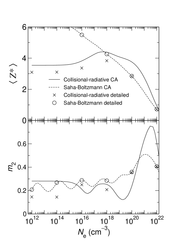
Figure 1: Average ionization $\left<Z^{\displaystyle*}\right>$ and second central moment $m_{2}=\left<(Z^{\displaystyle*}-\left<Z^{\displaystyle*}\right>)^{2}\right>$ for a 10-eV neon plasma, in the detailed level scheme (symbols) and in configuration average (lines). Populations are computed either with the collisional-radiative code or with the Saha-Boltzmann equation.

In figure 1 are presented the average charge $\left<Z^{\displaystyle*}\right>$ and the second central moment $m_{2}$ (IV.1) for a 10-eV neon plasma, both in the detailed-level scheme and in the CA approximation. The figure includes Saha-Boltzmann results too. For densities large enough (at least $10^{20}\text{ electrons/cm}^{3}$ ), the detailed data obtained with the collisional-radiative code (crosses) are identical to the Saha-Boltzmann values (circles), indicating that LTE is then reached. One notes that Saha-Boltzmann data are almost identical in the detailed (circles) and the CA case (dashed line). This indicates that the averaging on energies then performed in the Saha-Boltzmann equation bears very little influence on populations. Conversely, the CA (crosses) and detailed (solid line) results obtained with the collisional-radiative system are significantly different, indicating that the averaging procedure on rate equations is not of little consequence. As expected the CA validity worsens at low $T_{\text{e}}$, the difference being $\left<Z^{\displaystyle*}_{\text{CA}}\right>-\left<Z^{\displaystyle*}_{\text{det}}\right>=0.92$ at $N_{\text{e}}=10^{20}\text{ cm}^{-3}$. As seen in the lower part of this figure, the second moment $m_{2}$ exhibits similar properties, e.g., concerning the LTE convergence in the detailed case and the collisional-radiative vs Saha-Boltzmann differences. One can easily check that, if few charge states are populated, when $\left<Z^{\displaystyle*}\right>$ is integer (resp. half-integer), $m_{2}$ is close to a minimum (resp. maximum). This explains the oscillations observed on this figure.

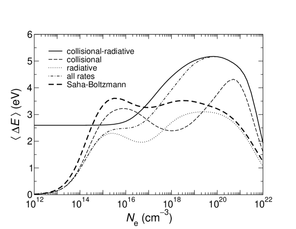
Figure 2: Average configuration energy dispersion $\left<\Delta E\right>=\sum_{\alpha}N_{\alpha}\Delta E_{\alpha}$ in a $T_{\text{e}}=10\text{ eV}$ neon plasma. $\Delta E_{\alpha}$ is the energy dispersion inside the configuration $\alpha$, and $N_{\alpha}$ is the $\alpha$-population calculated with various rate-equation systems and with Saha-Boltzmann equation. The smaller these dispersions are versus $T_{\text{e}}$, the better is assumed to be the configuration average approximation.

In order to check the breakdown of CA validity without performing any detailed-level computation, a first criterion is provided by the average-energy dispersion (II.4). The first member of this equation is plotted as a function of $N_{\text{e}}$ in figure 2. It appears that the energy dispersion $\left<\Delta E\right>$ is here rather large, in the 2–5 eV range, to be compared to $T_{\text{e}}=10\text{ eV}$. Furthermore, the dispersion calculated with the collisional-radiative system solution is always greater than 1.9 eV, and peaks at 5.2 eV for $N_{\text{e}}=10^{20}\text{ cm}^{-3}$ which is precisely the maximum of the CA versus detailed difference on $\left<Z^{\displaystyle*}\right>$. If one estimates that the criterion (II.4) is not fulfilled for $\left<\Delta E\right>=2.6\text{ eV}$, it has the expected behavior. The energy dispersion $\left<\Delta E\right>$ may also be computed with populations from the Saha-Boltzmann equation or from the modified rate equations proposed in subsection II.3. As seen in figure 2, it is smaller than the dispersion from collisional-radiative solution (except in the $N_{\text{e}}\simeq 10^{15}\text{--}10^{16}\text{ cm}^{-3}$ range) and particularly for electron densities well below $10^{13}\text{ cm}^{-3}$ where this quantity tends to zero. This can be explained as follows, e.g., for the “collisional” rate equations. Ignoring the collisional excitation and de-excitation processes that do not change the ionization degree, the ionization balance depends on the collisional ionization rate from the charge state $z$ to $z+1$, $R^{\text{(ci)}}N_{z}N_{\text{e}}$, and on the three-body recombination process from $z\!+\!1$ to $z$, $R^{\text{(3br)}}N_{z+1}N_{\text{e}}^{2}$. At equilibrium, this gives a population ratio $N_{z}/N_{z+1}\sim N_{\text{e}}R^{\text{(3br)}}/R^{\text{(ci)}}$, vanishing at low $N_{\text{e}}$. Therefore the highest charges are then favored: it should be 10 at very low $N_{\text{e}}$, but since the closed-shell $1s^{2}$ Ne ix is very stable, one gets $\left<Z^{\displaystyle*}\right>=8$ over a large range of densities. A similar analysis may be performed for the “radiative” equilibrium where photoionization and radiative recombination are included. In these cases, since the mainly populated configuration is $1s^{2}$ with $\Delta E_{\alpha}=0$, the resulting average energy dispersion is very small. In the contrary, in the collisional-radiative case, the low-density balance (coronal plasmas) is governed by collisional ionization and radiative recombination and then one gets a constant nonzero $N_{z}/N_{z+1}$, and therefore $\left<Z^{\displaystyle*}\right>\neq 8$. For this rate system, the average dispersion $\left<\Delta E\right>$ is nonzero, as seen in figure 2.

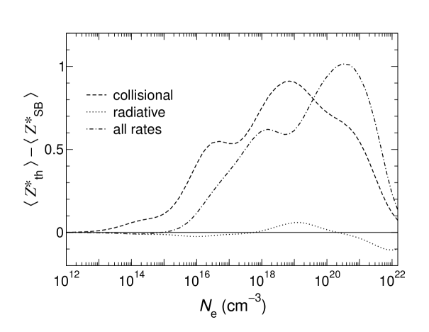
Figure 3: Difference between the average charge calculated with various rate-equation systems and the average charge obtained from the Saha-Boltzmann equation. Calculations are performed in a 10-eV neon plasma in the configuration average scheme.

To check how the proposed criterion based on the solution of a partial rate equations behaves, one may consider the variation of $\left<Z^{\displaystyle*}_{\text{th}}\right>-\left<Z^{\displaystyle*}_{\text{SB}}\right>$ displayed in figure 3. It is expected that, when this difference is large, the CA approximation will fail. It first appears that the “radiative” solution as proposed in section III remain rather close to the Saha-Boltzmann solution, and cannot in this case provide a test for the CA validity. However, the “complete” solution involving all the microreversible rates (collisional, autoionization and radiative in a fictive Planck field) presents a maximum difference on $\left<Z^{\displaystyle*}_{\text{all}}\right>-\left<Z^{\displaystyle*}_{\text{SB}}\right>$ at $N_{\text{e}}=3\times 10^{20}\text{ cm}^{-3}$, precisely where the CA-detailed departure is maximum. Furthermore, this $\left<Z^{\displaystyle*}_{\text{all}}\right>-\left<Z^{\displaystyle*}_{\text{SB}}\right>$ value, close to 1, provides then a reasonable quantitative estimate of the CA-detailed difference, at variance with the simple criterion (II.4). The drawback of the present criterion lies here once again the the low-density region, where all the computed $\left<Z^{\displaystyle*}\right>$ are close to 8, and therefore the differences plotted on figure 3 tend to zero. In this particular case, one must resort to the usual energy criterion (II.4). This is an opposite situation to the carbon case Poirier and de Gaufridy de Dortan (2007): for instance, if $N_{\text{e}}=10^{12}\text{ cm}^{-3}$ and $T_{\text{e}}=1\text{ eV}$, while the energy criterion (II.4) is fulfilled by large, the average charge difference $\left<Z^{\displaystyle*}_{\text{coll}}\right>-\left<Z^{\displaystyle*}_{\text{SB}}\right>$ is close to 1, indicating that CA approximation does fail.

An alternate analysis may be performed on the second or third central moments computed with the solution with rates as defined in section III and compared to the analogous moments from Saha-Boltzmann solution. It has been checked that the conclusions remain similar, with a maximum difference around $N_{\text{e}}=10^{21}\text{ cm}^{-3}$. Again the “radiative” solution remain closer to Saha-Boltzmann than the “collisional” or “full” solution.

V Conclusion

It has been demonstrated that the configuration-average validity for collisional-radiative rates, which leads to considerable simplification of these equation systems, may be controlled by comparison of several variants of a modified rate system with Saha-Boltzmann solution. These tests have been performed on the average ionization degree as well as the second and third central moments. The radiative test appears to be easier to verify than the collisional or complete tests: This demonstrates that the CA breakdown is induced mainly by large dispersions in collisional rates inside a given pair of configurations and not in radiative rates. Tests have been performed in carbon and neon, where atomic and collisional data were provided by the HULLAC code. Going from C to Ne amounts to increase the number of levels from 1782 to 4638 (and from 150 to 291 configurations) without impairing the efficiency of the proposed test. A detailed analysis in a carbon plasma has proven that failure of the CA at $T_{\text{e}}=1\text{ eV}$ may be correctly detected by the test based on the modified-rate system, while failure of CA in a 10 eV-neon plasma at low density is better diagnosed by the intuitive criterion based on the average energy dispersion inside a configuration. This situation prevails when the modified-rate equations solution is dominated by closed-shell ions such as Neix. Therefore, both criteria appear quite complementary. Nevertheless, the criterion based on the average charge difference may provide a semi-quantitative estimate of the CA-versus-detailed charge difference, at variance with the dispersion energy criterion. Further developments include the use of such systems in the determination of physically important quantities such as radiative losses, the opacity, and the emission of non-equilibrium plasmas Peyrusse (2001); Chung et al. (2006); Colgan et al. (2006). It is interesting to check how the various forms of the present criterion can control the relevance of CA approximation when dealing with such radiative properties. As a possible example of application, a configuration averaged code based on the HULLAC suite has been recently applied in our group to the EUV emission of xenon plasmas de Gaufridy de Dortan (2006).

Appendix A Validity of the configuration average: an example

In the special case where the rates inside every pair of configurations are proportional to the final level degeneracy

$$R_{ij}=R_{\alpha\beta}\frac{g_{j}}{g_{\beta}}\quad\forall i\in\alpha,j\in\beta,$$ (A.1)

the solution of the detailed-level rate equations can be straightforwardly derived from the solution of the configuration-average rate equations. Let us assume that the populations ${\bar{N_{\alpha}}}$ are the solutions of the CA rate equation (II.3). If we define level populations according to

$$\bar{N_{i}}=\bar{N_{\alpha}}\frac{g_{i}}{g_{\alpha}},\ \bar{N_{j}}=\bar{N_{\beta}}\frac{g_{j}}{g_{\beta}}\quad i\in\alpha,j\in\beta$$ (A.2)

then it is easy to show that such populations obey the detailed rate equation (II.1). One has according to (A.1) and (A.2)

$$\sum_{\begin{subarray}{c}j\\ j\neq i\end{subarray}}\left(-R_{ij}\bar{N_{i}}+R_{ji}\bar{N_{j}}\right)=\sum_{\begin{subarray}{c}j\\ j\neq i\end{subarray}}\left(-R_{\alpha\beta}\frac{g_{i}g_{j}}{g_{\alpha}g_{\beta}}\bar{N_{\alpha}}+R_{\beta\alpha}\frac{g_{j}g_{i}}{g_{\beta}g_{\alpha}}\bar{N_{\beta}}\right)$$ (A.3)

where $\alpha$ (resp. $\beta$) is the configuration containing $i$ (resp. $j$). In the above sum, when the level $j$ belongs to the same configuration as $i$ ($\beta=\alpha$), the $j$-term vanishes identically; when $j$ belongs to another configuration ($\beta\neq\alpha$), the sum over $j\notin\alpha$ may be written $\sum_{\beta\neq\alpha}\sum_{j\in\beta}$ and then, since $\sum_{j\in\beta}g_{j}/g_{\beta}=1$, one gets after performing the $j$-sum

$$\sum_{\begin{subarray}{c}j\\ j\neq i\end{subarray}}\left(-R_{ij}\bar{N_{i}}+R_{ji}\bar{N_{j}}\right)=\frac{g_{i}}{g_{\alpha}}\sum_{\begin{subarray}{c}\beta\\ \beta\neq\alpha\end{subarray}}\left(-R_{\alpha\beta}\bar{N_{\alpha}}+R_{\beta\alpha}\bar{N_{\beta}}\right)=0$$ (A.4)

because of the $\bar{N_{\alpha}},\bar{N_{\beta}}$ satisfy the CA rate equations (II.3). In a case where (A.1) is fulfilled the microreversibility-based (or “thermodynamic”) test checking the CA validity proposed in this paper is satisfied: the populations obtained with partial rate equations are identical to Saha-Boltzmann.

Appendix B Average of microreversible rates when the energy dispersion is small versus the electron thermal energy

In this appendix it is proved that, if the energy dispersion inside every configuration is much smaller than the electron thermal energy (II.7), then the microreversibility condition on detailed levels implies microreversibility on configuration-averaged rates too. Let us assume that the processes $p$ and $q$ (e.g., collisional ionization and three-body recombination) obey the microreversibility condition

$$R_{ij}^{(p)}N_{i}^{\text{SB}}=R_{ji}^{(q)}N_{j}^{\text{SB}}$$ (B.1)

for every $i\in\alpha,j\in\beta$, where the populations $N_{i}^{\text{SB}},N_{j}^{\text{SB}}$ obey the Saha-Boltzmann equation (II.6). Then, using the average rate definition (II.2) one gets

$$\begin{split}R_{\alpha\beta}^{(p)}&=\frac{1}{g_{\alpha}}\sum_{\begin{subarray}{c}i\in\alpha\\ j\in\beta\end{subarray}}g_{i}\frac{N_{j}^{\text{SB}}}{\vrule width=0.0pt,height=9.68747pt,depth=4.30554ptN_{i}^{\text{SB}}}R_{ji}^{(q)}\\ &=\frac{\Theta^{s}}{g_{\alpha}}\sum_{\begin{subarray}{c}i\in\alpha\\ j\in\beta\end{subarray}}g_{j}e^{(-E_{ji}/T_{\text{e}})}R_{ji}^{(q)}\end{split}$$ (B.2)

and if it is possible to identify the energy difference $E_{ji}$ with the difference of the average configuration energy

$$\left|E_{ji}-E_{\beta\alpha}\right|\ll T_{\text{e}}$$ (B.3)

then after substitution of $E_{\beta\alpha}$ to $E_{ji}$, the rate expression (B.2) involves the Saha-Boltzmann ratio of the configuration populations

$$\begin{split}R_{\alpha\beta}^{(p)}&\simeq\frac{\Theta^{s}}{g_{\alpha}}e^{-E_{\beta\alpha}/T_{\text{e}}}\sum_{\begin{subarray}{c}i\in\alpha\\ j\in\beta\end{subarray}}g_{j}R_{ji}^{(q)}\\ &=\frac{g_{\beta}}{g_{\alpha}}\Theta^{s}e^{-E_{\beta\alpha}/T_{\text{e}}}R_{\beta\alpha}^{(q)}=\frac{N_{\beta}^{\text{SB}}}{N_{\alpha}^{\text{SB}}}R_{\beta\alpha}^{(q)}\end{split}$$ (B.4)

where the Saha-Boltzmann populations $N_{\alpha}^{\text{SB}}$ computed with average energies have been introduced. This means that, in this case, the microreversibility condition holds for configurations too. However, conditions (II.7) or (B.3) assume that the maximum energy dispersion on every pair of configurations must be smaller than $T_{\text{e}}$, which is a much stronger condition than (II.4) which only requires the average energy dispersion to be much less than $T_{\text{e}}$.

Tables

Table 1: Number of configurations and levels considered for the collisional-radiative calculations in the neon plasma. For Nei to Neviii, the included configurations are $1s^{2}\{2s2p\}^{k}$, $1s^{2}\{2s2p\}^{k-1}Nl$, where $\{2s2p\}^{j}$ stands for $2s^{2}2p^{j-2},2s2p^{j-1},2p^{j-2}$. The configurations considered in Neix are $1s^{2}\text{ and }1sNl$, those in Nex are $Nl$. One has $N\leq 5,l\leq N-1$ for each ion. The Ci–Cvii computations include configurations isoelectronic to Nev–Nexi respectively.

Ion	Nei	Neii	Neiii	Neiv	Nev	Nevi	Nevii	Neviii	Neix	Nex	Nexi	Total
Configurations	25	38	39	39	39	39	27	14	15	15	1	291
Levels	157	501	994	1204	1004	513	166	24	49	25	1	4638

Table 2: Average ionization level in a neon plasma at $T_{e}=25\text{ eV}$ and 50 eV. DLA is a detailed model, while MOST is based upon superconfiguration averaging Hansen et al. (2006). The code “hybrid” is a partially detailed and partially averaged model based on FAC code Hansen et al. (2007); Gu (2003). The last two columns are the present results, in detailed and configuration average form.

$T_{\text{e}}$	$N_{\text{e}}\text{(cm${}^{-3}$)}$	DLA	MOST	hybrid	detail	CA
25	$10^{16}$	5.247	5.87	5.227	5.530	5.712
	$10^{18}$	6.050	6.17	6.101	6.352	6.406
	$10^{20}$	6.158	6.23	6.291	6.183	6.303
	$10^{22}$	3.403	3.78	4.200	3.083	3.248
50	$10^{16}$	7.625	7.45	7.618	7.604	7.607
	$10^{18}$	7.739	7.80	7.797	7.791	7.791
	$10^{20}$	7.901	7.90	7.917	7.905	7.905
	$10^{22}$	6.275	6.31	6.706	6.134	6.194

Table 3: Accuracy check of the collisional-radiative (CR) detailed-level solution for neon at $T_{\text{e}}=10\text{ eV}$. The average charge $\left<Z^{\displaystyle*}\right>$ is calculated using three kinds of microreversible rates: collisional rates ($\left<Z^{\displaystyle*}_{\text{coll}}\right>$), radiative rates including absorption and stimulated emission in a Planckian field ($\left<Z^{\displaystyle*}_{\text{rad}}\right>$), all these rates plus autoionization and dielectronic recombination rates ($\left<Z^{\displaystyle*}_{\text{all}}\right>$). $\left<Z^{\displaystyle*}_{\text{SB}}\right>$ is the average charge at thermal equilibrium as derived from Saha-Boltzmann and should be equal to the previous $\left<Z^{\displaystyle*}\right>$ values at infinite numerical accuracy. The additional test $\delta_{\text{rad}}$ (resp. $\delta_{\text{col}}$, $\delta_{\text{all}}$,) is the maximum difference on the ion-level populations between the “radiative”, (resp “collisional”, “complete”) system and the Saha-Boltzmann solution.

$N_{e}\text{(cm${}^{-3}$)}$	$\left<Z^{\displaystyle*}_{\text{rad}}\right>$	$\left<Z^{\displaystyle*}_{\text{coll}}\right>$	$\left<Z^{\displaystyle*}_{\text{all}}\right>$	$\left<Z^{\displaystyle*}_{\text{SB}}\right>$	$\delta_{\text{rad}}$	$\delta_{\text{col}}$	$\delta_{\text{all}}$
$10^{12}$	7.712640377	7.712640378	7.712640377	7.712640377	$2.0\times 10^{-10}$	$2.7\times 10^{-9}$	$1.5\times 10^{-10}$
$10^{14}$	6.639625837	6.639625830	6.639625838	6.639625838	$1.9\times 10^{-10}$	$3.4\times 10^{-9}$	$4.6\times 10^{-11}$
$10^{16}$	5.491015460	5.491015458	5.491015465	5.491015460	$1.9\times 10^{-12}$	$7.2\times 10^{-10}$	$1.3\times 10^{-9}$
$10^{18}$	4.260724652	4.260724657	4.260724656	4.260724652	$6.5\times 10^{-13}$	$1.5\times 10^{-9}$	$1.3\times 10^{-9}$
$10^{20}$	2.847355968	2.847355980	2.847355979	2.847355968	$2.1\times 10^{-14}$	$1.1\times 10^{-9}$	$1.2\times 10^{-9}$
$10^{22}$	0.719532736	0.719535868	0.719535378	0.719532736	$4.1\times 10^{-14}$	$6.9\times 10^{-7}$	$7.0\times 10^{-7}$

Table 4: Average ionization stage in a 10 eV-carbon plasma as a function of the electron density $N_{\text{e}}$. The last two columns are the configuration-average (CA) charge and the detailed-level charge derived from the collisional-radiative (CR) equations. The discrepancy between these values is correlated to the discrepancy between the Saha-Boltzmann charge (column 5) and the average charge derived from various modified rate-equation systems: collisional rates (column 2), radiative rates including a fictive Planckian field (column 3), all these rates plus autoionization (column 4). Data in columns 2–5 are obtained in the CA framework.

$N_{\text{e}}$	Modified-rate system				CR system
$(\text{cm}^{-3})$	$\left<Z^{\displaystyle*}_{\text{coll}}\right>$	$\left<Z^{\displaystyle*}_{\text{rad}}\right>$	$\left<Z^{\displaystyle*}_{\text{all}}\right>$	$\left<Z^{\displaystyle*}_{\text{SB}}\right>$	$\left<Z^{\displaystyle*}_{\text{CA}}\right>$	$\left<Z^{\displaystyle*}_{\text{det}}\right>$
$10^{12}$	4.000003693	4.000003671	4.000003671	4.000004022	3.7363	3.7441
$10^{14}$	3.999998275	3.999998275	3.999998275	3.999998278	3.7563	3.7616
$10^{16}$	3.999823807	3.999823806	3.999823806	3.999823805	3.9273	3.9273
$10^{18}$	3.982626435	3.982615120	3.982627955	3.982613441	3.9679	3.9679
$10^{20}$	3.225872703	3.197765566	3.230477092	3.194905628	3.2282	3.1902
$10^{22}$	1.052601006	0.689418858	1.069768540	0.717721378	1.0698	0.7113

Table 5: Average ionization degree in a neon plasma at $T_{\text{e}}=30\text{ eV}$ with respect to the electron density $N_{\text{e}}$. Column 2 involves detailed levels, while columns 3–7 contain charges which are computed in the configuration average scheme. Columns 2 and 3 are the collisional-radiative solution, while columns 4–6 are variants of “microreversibility check”, based on a collisional, radiative, or complete set of rates respectively. The closer these values are with respect to the Saha-Boltzmann $\left<Z^{\displaystyle*}\right>$ value (column 7), the better is assumed to be the configuration average. Column 8 is the average energy dispersion of levels inside a configuration with a ponderation by the collisional-radiative configuration populations.

$N_{\text{e}}$	CR system		Modified rate system			Saha-	$\left<\Delta E_{\text{CR}}\right>$
$(\text{cm}^{-3})$	Detailed	CA	Collisional	Radiative	Complete	Boltzmann	(eV)
$10^{12}$	5.7919	5.6236	8.000009396	8.000009460	8.000009460	8.000010081	0.069
$10^{14}$	5.7911	5.6540	7.999998415	7.999998416	7.999998416	7.999998422	0.164
$10^{16}$	6.2120	6.3134	7.999832154	7.999832154	7.999832154	7.999832154	2.18
$10^{18}$	6.8256	6.8456	7.983410902	7.983409743	7.983409658	7.983407736	1.13
$10^{20}$	6.9131	6.9400	7.180274366	7.172115334	7.180822653	7.168028134	0.97
$10^{22}$	3.6140	3.6603	4.471505865	4.090408345	4.436454002	4.047538516	5.92

Table 6: Second central moment $\left<(Z^{\displaystyle*}-\left<Z^{\displaystyle*}\right>)^{2}\right>$ in a neon plasma at $T_{\text{e}}=30\text{ eV}$ as a function of $N_{\text{e}}$. Refer to Table 5 for details. The average energy dispersion $\left<\Delta E_{\text{CR}}\right>$ is not repeated.

$N_{\text{e}}$	CR system		Modified rate system			Saha-
$(\text{cm}^{-3})$	Detailed	CA	Collisional	Radiative	Complete	Boltzmann
$10^{12}$	0.6128	0.5283	0.000009430	0.000009494	0.000009494	0.000010114
$10^{14}$	0.6137	0.5433	0.000001773	0.000001773	0.000001773	0.000001780
$10^{16}$	0.5043	0.4528	0.000167828	0.000167828	0.000167828	0.000167829
$10^{18}$	0.3288	0.3137	0.016394148	0.016396461	0.016396557	0.016400426
$10^{20}$	0.4700	0.4377	0.442653567	0.456411086	0.440578198	0.459907235
$10^{22}$	0.7707	0.7484	0.785410789	0.787926179	0.811753013	0.823178341

Table 7: Third central moment $\left<(Z^{\displaystyle*}-\left<Z^{\displaystyle*}\right>)^{3}\right>$ in a neon plasma at $T_{\text{e}}=30\text{ eV}$ as a function of $N_{\text{e}}$. Refer to Table 5 for details.

$N_{\text{e}}$	CR system		Modified rate system			Saha-
$(\text{cm}^{-3})$	Detailed	CA	Collisional	Radiative	Complete	Boltzmann
$10^{12}$	$-$0.0647	$-$0.2229	$-$0.000009396	$-$0.000009460	$-$0.000009460	$-$0.000010080
$10^{14}$	$-$0.0685	$-$0.2146	$-$0.000001585	$-$0.000001584	$-$0.000001584	$-$0.000001578
$10^{16}$	$-$0.0500	$-$0.0416	$-$0.000167786	$-$0.000167786	$-$0.000167787	$-$0.000167787
$10^{18}$	$-$0.0289	$-$0.0212	$-$0.016009480	$-$0.016014093	$-$0.016014161	$-$0.016021878
$10^{20}$	$-$0.0844	$-$0.0508	$-$0.097745732	$-$0.118986694	$-$0.093018605	$-$0.119420248
$10^{22}$	$-$0.2376	$-$0.3694	$-$0.125419985	$-$0.024429621	$-$0.109647319	$-$0.010892532

Figures

References

- Bauche-Arnoult et al. (1979) C. Bauche-Arnoult, J. Bauche, and M. Klapisch, Phys. Rev. A 20, 2424 (1979).
- Bauche-Arnoult et al. (1982) C. Bauche-Arnoult, J. Bauche, and M. Klapisch, Phys. Rev. A 25, 2641 (1982).
- Bauche et al. (1988) J. Bauche, C. Bauche-Arnoult, and M. Klapisch, Adv. At. Mol. Phys. 23, 131 (1988).
- Bauche-Arnoult et al. (1985) C. Bauche-Arnoult, J. Bauche, and M. Klapisch, Phys. Rev. A 31, 2248 (1985).
- Bar-Shalom et al. (1989) A. Bar-Shalom, J. Oreg, W. H. Goldstein, D. Shvarts, and A. Zigler, Phys. Rev. A 40, 3183 (1989).
- Bar-Shalom et al. (1997) A. Bar-Shalom, J. Oreg, and M. Klapisch, Phys. Rev. E 56, R70 (1997).
- Peyrusse (1999) O. Peyrusse, J. Phys. B 32, 683 (1999).
- Bar-Shalom et al. (2000) A. Bar-Shalom, J. Oreg, and M. Klapisch, J. Quant. Spectrosc. Radiat. Transfer 65, 43 (2000).
- Peyrusse (2001) O. Peyrusse, J. Quant. Spectrosc. Radiat. Transfer 71, 571 (2001).
- Bauche et al. (2004) J. Bauche, C. Bauche-Arnoult, and K. B. Fournier, Phys. Rev. E 69, 026403 (2004).
- Busquet (1993) M. Busquet, Phys. Fluids B 5, 4191 (1993).
- Bauche and Bauche-Arnoult (2000) J. Bauche and C. Bauche-Arnoult, J. Phys. B 33, L283 (2000).
- Hansen et al. (2006) S. Hansen, K. B. Fournier, C. Bauche-Arnoult, J. Bauche, and O. Peyrusse, J. Quant. Spectrosc. Radiat. Transfer 99, 272 (2006).
- Hansen et al. (2007) S. Hansen, J. Fournier, C. Bauche-Arnoult, and M. F. Gu, High Energy Density Physics 3, 109 (2007).
- Nishihara et al. (2006) K. Nishihara, A. Sasaki, A. Sunahara, and T. Nishikawa, EUV Sources for Lithography (SPIE Press, Bellingham, Washington USA, 2006), chap. 11, pp. 339–370.
- O’Sullivan et al. (2006) G. O’Sullivan, A. Cummings, P. Dunne, P. Hayden, L. McKinney, N. Murphy, and J. White, EUV Sources for Lithography (SPIE Press, Bellingham, Washington USA, 2006), chap. 5, pp. 149–173.
- Al Rabban et al. (2006) M. Al Rabban, M. Richardson, H. Scott, F. Gilleron, M. Poirier, and T. Blenski, EUV Sources for Lithography (SPIE Press, Bellingham, Washington USA, 2006), chap. 10, pp. 299–337.
- Hakel et al. (2006) P. Hakel, M. Sherrill, S. Mazevet, J. J. Abdallah, J. Colgan, D. Kilcrease, N. Magee, C. Fontes, and H. Zhang, J. Quant. Spectrosc. Radiat. Transfer 99, 265 (2006).
- Rodríguez et al. (2006) R. Rodríguez, J. Gil, R. Florido, J. Rubiano, P. Martel, and E. Mínguez, J. Phys. IV 133, 981 (2006).
- Chung et al. (2005) H. K. Chung, M. H. Chen, W. Morgan, Y. Ralchenko, and R. Lee, High Energy Density Physics 1, 3 (2005).
- Faussurier et al. (2001) G. Faussurier, C. Blancard, and E. Berthier, Phys. Rev. E 63, 026401 (2001).
- Bowen et al. (2003) C. Bowen, A. Decoster, C. J. Fontes, K. B. Fournier, O. Peyrusse, and Y. Ralchenko, J. Quant. Spectrosc. Radiat. Transfer 81, 71 (2003).
- Bowen et al. (2006) C. Bowen, R. W. Lee, and Y. Ralchenko, J. Quant. Spectrosc. Radiat. Transfer 99, 102 (2006).
- Poirier and de Gaufridy de Dortan (2007) M. Poirier and F. de Gaufridy de Dortan, Journal of Applied Physics 101, 063308 (2007).
- Busquet (2007) M. Busquet, High Energy Density Physics 3, 48 (2007).
- Goett et al. (1980) S. J. Goett, R. E. H. Clark, and D. H. Sampson, At. Data Nucl. Data Tables 25, 185 (1980).
- Bar-Shalom et al. (2001) A. Bar-Shalom, M. Klapisch, and J. Oreg, J. Quant. Spectrosc. Radiat. Transfer 71, 169 (2001).
- Gilleron et al. (2003) F. Gilleron, M. Poirier, T. Blenski, M. Schmidt, and T. Ceccotti, J. Appl. Phys. 94, 2086 (2003).
- van Regemorter (1962) H. van Regemorter, Astrophys. J. 136, 906 (1962).
- Mewe (1972) R. Mewe, Astron. Astrophys. 20, 215 (1972).
- Gu (2003) M. F. Gu, Astrophys. J. 582, 1241 (2003).
- Chung et al. (2006) H. K. Chung, K. B. Fournier, and R. W. Lee, High Energy Density Physics 2, 7 (2006).
- Colgan et al. (2006) J. Colgan, C. J. Fontes, and J. Abdallah Jr., High Energy Density Physics 2, 90 (2006).
- de Gaufridy de Dortan (2006) F. de Gaufridy de Dortan, Tech. Rep. CEA-R-6115, CEA (2006).