Thermal critical behavior and universality aspects of the three-dimensional random-field Ising model

Abstract

The three-dimensional bimodal random-field Ising model is investigated using the N-fold version of the Wang-Landau algorithm. The essential energy subspaces are determined by the recently developed critical minimum energy subspace technique, and two implementations of this scheme are utilized. The random fields are obtained from a bimodal discrete $(\pm\Delta)$ distribution, and we study the model for various values of the disorder strength $\Delta$, $\Delta=0.5,\;1,\;1.5$ and $2$, on cubic lattices with linear sizes $L=4-24$. We extract information for the probability distributions of the specific heat peaks over samples of random fields. This permits us to obtain the phase diagram and present the finite-size behavior of the specific heat. The question of saturation of the specific heat is re-examined and it is shown that the open problem of universality for the random-field Ising model is strongly influenced by the lack of self-averaging of the model. This property appears to be substantially depended on the disorder strength.

1 Introduction

The random-field Ising model (RFIM) imry75 is one of the most studied glassy magnetic models natter88 ; belang91 ; rieger95a ; belang98 , mainly because of its interest as a simple frustrated system. The Hamiltonian of the system is:

$$\mathcal{H}=-J\sum_{<i,j>}S_{i}S_{j}-\sum_{i}h_{i}S_{i},$$ (1)

where the $S_{i}=\pm 1$ are Ising spins, $J$ is the interaction energy between nearest neighbors, which we take to be positive so that the model is ferromagnetic and $h_{i}$ are the random fields (RF’s). In this paper the values $h_{i}$ are taken from a bimodal distribution of the form:

$$P(h_{i})=\frac{1}{2}\delta(h_{i}-\Delta)+\frac{1}{2}\delta(h_{i}+\Delta),$$ (2)

with $\Delta$ the disorder strength, also called randomness of the system. Various different RF probability distributions have been studied in the past hartmann01 ; hartmann99 ; newman96 ; sourlas99 , such as the Gaussian distribution, the wide bimodal distribution (with a Gaussian width), and the bimodal distribution considered also here.

In spite of many years of study, the critical behavior of the three-dimensional (3D) RFIM has been a matter of several debates and is still controversial. One of the early disagreements was the question of whether the model undergoes a phase transition from a high temperature paramagnetic phase to a low temperature ferromagnetic one, for some range of the randomness $\Delta$. The work of Parisi and Sourlas parisi78 introduced the notion of dimensional reduction, indicating that the critical behavior of the RFIM in $d$ dimensions, at sufficiently low randomness, should be identical to that of the well-known normal Ising model in $d-2$ dimensions. This in turn indicated that the model should not exhibit a phase transition in 3D or fewer. However, a different argument based on the droplet theory of domain wall energies in the ferromagnetic state grinstein82 , suggested that a phase transition should exist in 3D for finite temperature and randomness. The whole puzzle has been largely cleared out by Imbrie imbrie84 and Bricmont and Kupiainen bricmont87 , who showed the existence of an ordered phase. Their arguments strongly supported the view that a phase transition in 3D exists, provided that the randomness is sufficiently small $(\Delta_{c}\simeq 2.3)$.

However, agreement over several fundamental issues is missing and the characterization of the phase transition is still unclear rieger95 . Despite the fact that most studies suggest a second-order transition rieger95 ; villain85 ; fisher85 ; bray85 ; ogielski86 ; ogielski86b , there are also indications of first-order or hybrid-order transition rieger95 ; mccay88 . Note also that the mean field theory aharony78 differentiates between a binary and a continuous randomness distribution, predicting for the former a tricritical point at which the transition becomes of the first-order, at high fields. However, it is now generally accepted that a new fixed point controls the behavior of RF ferromagnets chayes86 ; cardy . The significance of this for the RFIM (in $d>2$) is that this new zero temperature random fixed point controls the whole critical line ($T_{c}(\Delta)$) and that the RF’s are always relevant. For disordered systems with weak randomness which couples to the local energy (such as random-site impurity or random-bond models) the crossover to a new random fixed point, depends on the Harris criterion cardy ; harris74 . According to this, the disorder is relevant if the correlation length exponent of the pure model ($\nu=\nu_{pure}$) satisfies the condition $d\nu<2$ and this condition may be stated, with the help of the hyper-scaling relation ($\alpha=2-d\nu$), as $\alpha>0$. Since the specific heat exponent of the 3D Ising model is positive, weak disorder should be expected to be relevant. In the case of the RFIM the type of disorder is much more severe, since the randomness couples to the local order-parameter and the crossover renormalization group eigenvalue is always positive cardy . The inequality $\nu\geq 2/d$, derived by Chayes et al. chayes86 for the correlation length exponent of a generic disordered system ($\nu=\nu_{random}$) would imply, using again hyper-scaling, a negative specific heat exponent ($\alpha<0$). However, it is believed that hyper-scaling is violated in the RFIM and the specific heat exponent $\alpha$ is related to $\nu$ by a modified hyper-scaling law $2-\alpha=(d-\theta)\nu$, where the exponent $\theta$ characterizes the scaling of the stiffness of the ordered phase at the critical point. Thus, the specific heat exponent of the RFIM is not restricted, by the above theoretical considerations, to be negative chayes86 .

A general sketch of the phase diagram of the RFIM is given in several papers hartmann01 ; newman96 ; itakura01 and will be also presented here in Sect. 3.3. At low temperatures and moderate values of randomness, the system is assumed to be in an ordered ferromagnetic phase, whereas in the opposite regime the system is paramagnetic. From the notions of the perturbative renormalization group (PRG) it is expected that the RF is the relevant perturbation at the pure $(\Delta=0)$ fixed point, and that the RF fixed point is at $T=0$. However, it is known that PRG fails for the RFIM and that a theoretical justification of universality for this and also other disordered systems is lacking natter88 ; belang91 ; sourlas99 ; parisi78 . Questions concerning the general characterization of the phase transition, the existence of an intermediate glassy phase itakura01 ; mezard92 ; mezard94 , the behavior of the renormalization group flow in the middle of the phase diagram itakura01 , and the dependence of the critical exponents on the randomness distribution and disorder strength are still open hartmann99 ; sourlas99 ; sourlas97 .

A relevant active and enigmatic issue concerns the behavior of the specific heat (see Ref. fytas06a and references therein). The specific heat of the RFIM can be experimentally measured and is of considerable theoretical interest. There is a strong disagreement in literature about the possible divergence or saturation of the specific heat. In studies supporting the scenario of saturation there is a discrepancy in the reported negative values of the critical exponent $\alpha$. Some of these later studies find strongly negative values, ranging from $\alpha=-1.5$ rieger93 to $\alpha=-0.5$ hartmann01 ; rieger95 ; nowak98 . In particular, Hartmann and Young hartmann01 recently found by a ground state technique the value $\alpha=-0.63\pm 0.07$, whereas Middleton and Fisher middle02 , using the same technique, estimated in marked disagreement $\alpha=-0.01\pm 0.09$.

From the experimental point of view, a true realization of the RFIM is hardly conceived. However, it has been shown that dilute antiferromagnets in uniform external field (DAFF) represent physical realizations of the RFIM fishman79 and a number of experiments investigated the phase transitions of such 3D systems belanger83 . These experiments have proven to be very difficult and their interpretation doubtful due to the extremely slow, glassy dynamics of the system. Experiments on DAFF, provided evidence of a second-order phase transition and a logarithmic singularity for the specific heat belanger85 . Note that recently, Barber and Belanger barber01 in their Monte Carlo study of a DAFF model reported also that their specific heat curve closely mimics a logarithmic peak. Their results are based on a large lattice $(L=128)$ but instead of sample averaging they have observed the behavior of only a few RF realizations. On the other hand, there is also experimental evidence karszewiski94 supporting the opposite view of a cusp-like singularity of the specific heat, in agreement with a saturating specific heat $(\alpha<0)$ as found in the studies of Refs. rieger95 ; rieger93 .

It has been pointed out that a strongly negative value of $\alpha$ causes serious difficulties with respect to the Rushbrooke relation: $\alpha+2\beta+\gamma\geq 2$ hartmann01 ; rieger95 ; nowak98 ; middle02 . Therefore, there have been several attempts hartmann01 ; villain85 ; fisher85 ; bray85 ; grinstein76 in order to find a consistent set of scaling relations to describe the critical behavior of the RFIM. Among the several scaling scenarios proposed sourlas99 ; mezard92 ; mezard94 ; sourlas97 ; nowak98 ; middle02 , the single second-order critical point behavior characterized by three scaling exponents middle02 seems to be consistent with a close to zero estimate for the specific heat exponent. Thus, the above described conflicting situation in literature concerning the divergence or saturation of the specific heat is one of the open important issues, whose implications on the critical behavior of the model are not understood.

The first step towards its resolution was taken recently by the present authors fytas06a ; fytas06b , where an extended numerical investigation of the 3D bimodal ($\Delta=2$) RFIM revealed the importance of the property of lack of self-averaging of the specific heat of the model, as well as the possibility of large-$L$ crossover phenomena in the scaling behavior of the specific heat of the model. Here, we extend our analysis for the values $\Delta=0.5,\;1$ and $2$ of the disorder strength below the critical value $\Delta_{c}$ in order to obtain a more comprehensive picture. To this end, we implement recently developed efficient Monte Carlo methods that directly calculate the density of states (DOS) of a classical statistical model. A brief overview of the numerical techniques used in the past for the RFIM are presented in the next Section, together with the necessary details of the methods used in our approach. The utilization of our recently proposed critical minimum energy subspace (CrMES) scheme malak04 to the RFIM is also explained. In Sect. 3 the new numerical results for the cases $\Delta=0.5,\;1$ and $\Delta=1.5$ are given and the phase diagram of the model is reproduced. The universality aspects of the model are discussed and found to support the scenario of violation of universality. Our conclusions are summarized in Sect. 4.

2 Numerical techniques

There are two distinct kinds of numerical approaches for the RFIM. In the first approach, traditional Monte Carlo methods are used to simulate the properties of the system at finite temperatures rieger95 ; ogielski86 ; rieger93 ; nowak98 ; barber01 ; metrop53 ; newman99 ; young86 . The second approach is grounded on the well-known belief that the critical behavior of the model is governed by the non trivial RF fixed point at $T=0$ middle02 ; dukov03 . In this case, graph theoretical algorithms hartmann99 ; swamy91 are used to calculate the ground states of the system for a sample of RF’s at different disorder strength. Using this later approach quite large lattices have been studied: $L\leq 80$ hartmann99 ; dukov03 , $L\leq 90$ sourlas99 , $L\leq 96$ hartmann01 and finally $L\leq 256$ middle02 . Yet, in the traditional Monte Carlo approach the sizes studied were restricted to the size $L\leq 16$ newman96 ; rieger95 ; rieger93 , $L\leq 20$ nowak98 and finally we may refer, as an exception, to the case $L=128$ in the study of Ref. barber01 for particular RF’s as mentioned in the introduction. From the $T=0$ numerical studies one obtains an accurate estimate of the critical randomness and from the finite temperature studies further information for the phase diagram may be derived. From the finite temperature approach one can also find, by extrapolation, a crude estimate for the critical randomness newman96 (see Sect. 3). It is worth noting that quite recently Wu and Machta, combining finite and zero temperature studies of the RFIM, reported strong correlations of ground states and thermal states near the critical line for given realizations of the disorder, supporting strongly the $T=0$ fixed point scenario wu05 .

In traditional Monte Carlo studies of the RFIM newman96 ; rieger93 ; ogielski86 ; rieger95 ; nowak98 the system is simulated in a restricted range of temperatures, appropriate for the location of the pseudocritical temperatures. However, single spin-flip methods, such as the Metropolis or the heat bath algorithms, face severe slowing down problems of equilibration and temperature averaging since the characteristic times may be exponentially large at low temperatures $(T<T_{c})$, as explained in Ref. newman96 . Moreover, the sample averaging process introduces new characteristic features and requires further computer resources. Indeed, the appropriate pseudocritical temperature for the RFIM is a strongly fluctuating quantity fytas06a , and this property amplifies the computer time requirements for its location. Hence, depending on the size of the lattice and the disorder strength, it is necessary to simulate the system for each RF realization in a quite wide temperature range, which is not even known in advance. To obtain a good approximation of the locations of the specific heat peaks, the temperature step must be chosen sufficiently small for, otherwise any interpolation scheme may miss the correct height of a possible sharp peak. In fact, this situation of a possible sharp peak, turns out for a significant number of RF’s fytas06a .

From the above discussion one should wonder whether the traditional Metropolis sampling could be trusted to provide even a moderate estimation plan, since it requires immense computer resources and faces all mentioned problems. The cluster flipping algorithm for the RFIM proposed by Dotsenko, Selke and Talapov dotsenko91 is a straightforward extension of the Wolff algorithm wolff89 , devised to overcome the slowing down effect and speed up the flip dynamics. A more efficient form of this algorithm, the limited cluster flip (LCF) algorithm, has been invented by Newman and Barkema newman96 and was used for the study of the Gaussian RFIM. Furthermore, these authors have combined the LCF algorithm with the generalized histogram method of Ferrenberg and Swendsen ferre98 which is a re-weighting scheme, using a restricted set of temperature measurements. This combination may be hopefully more reliable for the location of the pseudocritical temperatures. Finally, a new cluster technique, that combines the replica-exchange method of Swendsen and Wang swend86 and the two-replica cluster method redner98 , was implemented by Machta, Newman, and Chayes machta00 where single realizations of the disorder strength were studied for sizes up to $L=24^{3}$.

Here, we employ a different strategy which utilizes the new and popular methods of efficient estimation of spectral degeneracies of classical statistical models newman99 ; ferre98 ; malak04b ; lee93 ; berg92 ; lima00 ; wang01 ; schul01 ; oliv96 ; zhou05 and the recently developed CrMES technique malak04 . This scheme has the merit of locating the pseudocritical temperatures by determining the DOS in the proper energy subspace by using simple algorithms in a unified implementation. Moreover, it avoids all the above problems, speeding up the simulations. Specifically, we use the multi-range Wang-Landau (WL) algorithm wang01 , and its N-fold version as presented by Schulz et al. schul01 . The accuracy of this scheme was discussed in Ref. fytas06a , where more details than those given below for the appropriate implementations can be found.

2.1 The Wang-Landau algorithm

For the application of the WL algorithm in a multi-range approach we follow the description of Schulz et al. schul01 , i.e., whenever the energy range is restricted we use the updating scheme $2$ in that paper. Consider the restriction of the random walk in a particular energy range $I=[E_{1},E_{2}]$ and assume that the random walk is at the border of the range $I$. Then, the next spin-flip attempt is determined by the modified Metropolis acceptance ratio:

$$A=\left\{\begin{array}[]{rr}\min\{1,G(E)/G(E+\Delta E)\},&\mbox{$(E+\Delta E)\in I$}\\ 0,&\mbox{$(E+\Delta E)\not\in I$}\end{array}\right.,$$ (3)

the random walk is not allowed to move outside of the energy range, and we always increment the histogram $H(E)\rightarrow H(E)+1$ and the DOS $G(E)\rightarrow G(E)*f_{j}$ after a spin-flip trial. Here, of course, $f_{j}$ is the value of the WL modification factor $f$ wang01 at the jth iteration, in the process $(f\rightarrow f^{1/2})$ of reducing its value to 1, where the detailed balance condition is satisfied. In all our simulations the WL modification or control parameter takes the initial value: $f_{j=1}=e\approx 2.71828...$. When starting a new iteration the control parameter is changed according to $f_{j+1}=\sqrt{f_{j}},j=1,2,\ldots,20$ wang01 . For the histogram flatness criterion, we use a flatness level $0.05$, as in previous studies malak04 ; malak04b .

2.2 The N-fold version of the Wang-Landau algorithm

For the bimodal RFIM is convenient to use an index $n$ to characterize directly the corresponding energy changes produced by the spin-flip process. The number of different classes for the N-fold version $n=1,...,\mathcal{N}$ depends on the value of the disorder strength $\Delta$. For example, consider the case $\Delta=1$. The possible energy changes are $\Delta E_{n}=\pm 14,\;\pm 10,\;\pm 6$ and $\pm 2$, and using an index $n=1,2,...,8$ corresponding to $8$ classes we can write $\Delta E_{n}=-14+(n-1)\cdot 4$. Note that, the RF value at the site in which the spin-flip is going to take place is also affecting the energy change. Denoting the populations of spins by $N_{n},\sum_{n}N_{n}=N$, where $N$ is the number of sites: $N=L^{3}$, the selection probability of a class, $P_{n}$, will be proportional to this number multiplied by the corresponding acceptance ratio. For the application of the algorithm in multi-range approach we follow the description of Schulz et al. schul01 for the N-fold version of the WL method. If the system is in a spin state with energy $E\in I$ and after the spin-flip is in a state with energy $E^{\prime}=E+\Delta E_{n}$, the selection of the class for the next spin-flip is obtained from the following malak04b :

$$P_{n}=N_{n}A_{n};\;A_{n}=\left\{\begin{array}[]{rr}\min\{1,G(E)/G(E^{\prime})\},&\mbox{$E^{\prime}\in I$}\\ 0,&\mbox{$E^{\prime}\not\in I$}\end{array}\right..$$ (4)

The average life time of a state, reflecting the number of attempts we expect the system to remain in its current state before moving to the new state, is $\Delta t=W/Z$ schul01 where:

$$W=\sum_{n}P_{n}.$$ (5)

The rest of details for the algorithms can be found in the original papers malak04b ; schul01 .

2.3 Implementation of the CrMES technique

The CrMES scheme malak04 uses only a small part $(\widetilde{E}_{-},\widetilde{E}_{+})$ of the energy space $(E_{min},E_{max})$ to determine the specific heat peaks. If $\widetilde{E}$ is the value of energy producing the maximum term in the partition function at the temperature of interest (say the pseudocritical temperature), the sums are restricted as follows:

$$C_{L}(\widetilde{E}_{-},\widetilde{E}_{+})=N^{-1}T^{-2}\left\{\widetilde{Z}^{-1}\sum_{\widetilde{E}_{-}}^{\widetilde{E}_{+}}E^{2}\exp{[\widetilde{\Phi}(E)]}-\right.$$

$$\left.\left(\widetilde{Z}^{-1}\sum_{\widetilde{E}_{-}}^{\widetilde{E}_{+}}E\exp{[\widetilde{\Phi}(E)]}\right)^{2}\right\}$$ (6)

and

$$\widetilde{\Phi}(E)=[S(E)-\beta E]-\left[S(\widetilde{E})-\beta\widetilde{E}\right];\;\;\widetilde{Z}=\sum_{\widetilde{E}_{-}}^{\widetilde{E}_{+}}\exp{[\widetilde{\Phi}(E)]},$$ (7)

where $(\widetilde{E}_{-},\widetilde{E}_{+})$ is the minimum dominant subspace satisfying the following accuracy criterion:

$$\left|\frac{C_{L}(\widetilde{E}_{-},\widetilde{E}_{+})}{C_{L}(E_{min},E_{max})}-1\right|\leq r.$$ (8)

In this paper we have used the accuracy criterion $r=10^{-4}$, which is extremely demanding compared to the relative errors produced in the specific heat, say by the WL method. It is also a very strict criterion for the present model, in view of the existing very large sample-to-sample fluctuations of the specific heat. A practical algorithmic approach for specifying the CrMES is fully described in Ref. malak04 . We may satisfy the specific heat accuracy criteria defined in equation (8) for any particular realization of the RF, by restricting the WL random walk in the corresponding critical energy subspace.

This restriction greatly facilitates our simulations without introducing additional errors. Since we don’t know in advance the CrMES for a specific realization of the RF we have two alternatives. The first option is to use an efficient prognostic method of identifying the CrMES for any particular realization of the RF by using the first stages of the WL method. For instance, one may try to estimate the CrMES from the first $12$ iterations in the process of reducing the WL modification factor $f$. To implement safely this option, one should be careful to use for the rest of WL iterations a much wider energy range than that predicted in the first $12$ iterations. The second option is to ‘guess’ (by using some convenient extrapolation method) a broad energy subspace that will cover the overlap of the CrMES for all RF’s in the sample. Implementing the second method is straightforward and has the advantage that the approximation for the specific heat curve of a particular RF realization is accurate in a wide temperature range including the pseudocritical temperature corresponding to the particular RF. This option (the second) was used for the cases $\Delta=0.5$ and $1$, whereas for $\Delta=1.5$ (and $2$ fytas06a ) both options were used, each for $50\%$ of the simulations (for a more detailed discussion see Ref. fytas06a ).

3 Results and analysis

3.1 Definitions and the property of self-averaging

For a disordered system we have to perform two distinct kinds of averaging. Firstly, for each RF realization the usual thermal average has to be carried out and secondly we have to average over the distribution of the random parameters. In effect, this means that we must generate and study quite large samples of RF’s. Following the methods outlined in Sect. 2.3 the thermal average for the specific heat is given by the approximations (2.3)-(8). Using large samples of RF’s we can estimate the relevant probability distributions of the location of the specific heat peaks. Let $C_{m}(T)$ denote the specific heat of a particular realization $m$ in a sample of $M$ realizations of the RF $(m=1,2,...,M)$. The pseudocritical temperature $T_{L}^{\ast}(C_{m}(T))$ depends on the realization of the RF and for large values of the randomness $\Delta$, is a strongly fluctuating quantity fytas06a . Let us also denote the locations of the specific heat peaks by $(C_{m}^{\ast},T_{L,m}^{\ast})$. It seems that, in all previous studies hartmann01 ; rieger95 ; rieger93 , the averaging process over an ensemble of RF’s was carried out on the curve of the averaged specific heat, without raising the question of whether this averaged curve is the proper statistical representative of the system. The peak of this averaged curve was then analyzed by using finite-size scaling relations. On the other hand, the work of Barber and Belanger barber01 , in which the behavior was observed for particular RF realizations, is a different route but it would be hard to accept this as an adequate alternative. A particular RF is not generally representative of the behavior of a large sample of RF’s.

Indeed, in previous papers hartmann01 ; rieger95 ; rieger93 ; nowak98 the following average has been considered for the specific heat:

$$[C]_{av}=\frac{1}{M}\sum_{m=1}^{M}C_{m}(T)$$ (9)

and the finite-size scaling behavior of the peak of this averaged curve has been studied, by assuming that the maximum $[C]^{\ast}_{av}=\max_{T}\{[C]_{av}\}$ and the corresponding pseudocritical temperature obey the scaling laws:

$$[C]_{av}^{\ast}\cong p+cL^{\alpha/\nu};\;\;T_{L}^{\ast}([C]_{av})\cong T_{c}+bL^{-1/\nu},$$ (10)

where $\alpha$ and $\nu$ are considered to be the specific heat and correlation length critical exponents, respectively. Note that, these averaged curves are very sensitive to the property of lack of self-averaging (see the discussion below) due to the fact that the corresponding thermodynamic quantities are characterized by broad distributions in the thermodynamic limit fytas06a .

It is clear that when studying random systems the only meaningful objects for investigating the finite-size scaling behavior are the distributions of various properties in ensembles of several realizations of the randomness. Hence, it is important to be able to ascertain to what extent are the results obtained from an ensemble of random realizations representative of the general class to which the system belongs. The answer hinges on the important issue of self-averaging. In a self-averaging system, a single very large system suffices to represent the ensemble; without self-averaging, a measurement performed in a single sample, no matter how large, does not give a meaningful result and must be repeated on many samples. In a Monte Carlo study of a self-averaging disordered system the number of samples needed to obtain the average $[Q]$ (e.g., $Q$ can be the energy, magnetization, specific heat, or susceptibility) to a given relative accuracy decreases with increasing $L$. On the other hand, in a non self-averaging system, the number of samples that must be simulated rises very strongly with $L$. If a quantity is not self-averaging, then we talk about lack of self-averaging and as explained the process of increasing $L$ does not improve the statistics. In other words, the sample-to-sample fluctuations remain large. The problem of self-averaging in the RFIM has been a matter of investigation over the last years fytas06a ; fytas06b ; parisi02 . A common measure characterizing the self-averaging property of a system based on the theory of finite-size scaling has been discussed by Binder binder88 and has been used for the study of some random systems wisem95 ; aharon96 . This measure inspects the behavior of a normalized square width quantity, defined as:

$$R_{Q}=\frac{V_{Q}}{[Q]^{2}},$$ (11)

where $V_{Q}=[Q^{2}]-[Q]^{2}$ is the sample-to-sample variance of the average $[Q]$. Here, $Q$ is used in respect of the specific heat $C_{m}^{\ast}$. According to the literature binder88 ; wisem95 ; aharon96 when the ratio $R_{Q}$ tends to a constant, the system is said to be non self-averaging and the corresponding distribution (say $P(Q)$) does not become sharp in the thermodynamic limit.

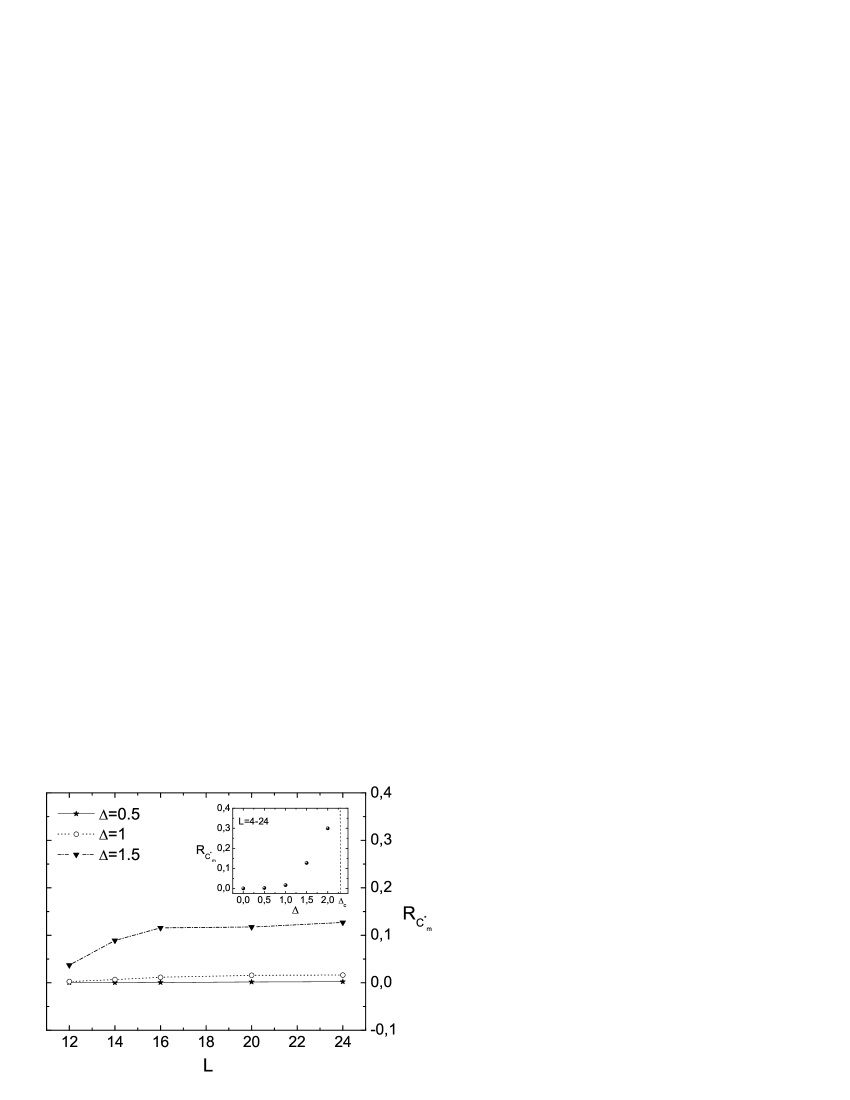
Figure 1: $L$-dependence of the ratio $R_{C_{m}^{\ast}}$ defined in equation (11) for $\Delta=0.5,\;1$ and $1.5$. The inset illustrates the variation of $R_{C_{m}^{\ast}}$ as a function of the disorder strength $\Delta$, including the value for the case $\Delta=2$ fytas06a .

In Ref. fytas06a it has been shown that the specific heat of the bimodal RFIM for the case $\Delta=2$ is characterized by the property of lack of self-averaging (see inset of figure 4 in Ref. fytas06a ). In analogy with the case $\Delta=2$ of Ref. fytas06a , we construct the ratio $R_{C_{m}^{\ast}}$ for the cases $\Delta=0.5,\;1$ and $1.5$ and plot the results in figure 1. The data presented for the cases $\Delta=0.5$ and $1$ are taken from $1000$ samples of RF’s for $L\leq 10$ and $400$ for $L=14-24$, while for the case $\Delta=1.5$ the samples of RF’s used were: $1000$ for $L\leq 12$ and $300$ for $L=12-24$.

From figure 1 we observe that for small values of the randomness $\Delta$ the ratio $R_{C_{m}^{\ast}}$ has values close to zero. In particular, for $\Delta=0.5$ the ratio $R_{C_{m}^{\ast}}$ shows a rather faint dependence on $L$ and is practically very close to zero. For this case, and possibly for even weaker RFs, it appears that $R_{C_{m}^{\ast}}\rightarrow 0$ and the property of self-averaging may be well obeyed. However, we know from our previous study for $\Delta=2$ that the above property is strongly violated, at the same lattice sizes, and that $R_{C_{m}^{\ast}}\rightarrow 0.3$ fytas06a . Thus, for strong disorder the behavior appears very different and the development of the increasing influence of the randomness $\Delta$ on the ratio $R_{C_{m}^{\ast}}$ can be seen in figure 1 and in particular from the corresponding inset. For the lattice sizes studied here ($L=4-24$) the ratio $R_{C_{m}^{\ast}}$ for the cases $\Delta\geq 1$ seems to increase with the lattice size and the estimated non-zero limiting values for $\Delta=1$ and $1.5$ are $R_{C_{m}^{\ast}}\rightarrow 0.016$ and $R_{C_{m}^{\ast}}\rightarrow 0.12$, respectively. However, the behavior of the specific heat is notoriously difficult even in simple pure models binder88 , and for the present model the already existing conflicting situation is an additional warning against drawing definite conclusions at these lattice sizes. It is quite possible that we are not yet in the regime of large enough $L$, where simple scaling laws would be expected to hold. For the case $\Delta=2$ we have already observed fytas06a that the system appears to crossover and change behavior for sizes $L>3$2 and we have suggested in that paper that the finite-size study should be extended to at least $L=80$ in order to have a more convincing picture. For the strengths studied here, $\Delta=0.5,\;1$ and $1.5$, we suspect that even much larger sizes would be needed in order to draw definite conclusions for the true asymptotic behavior.

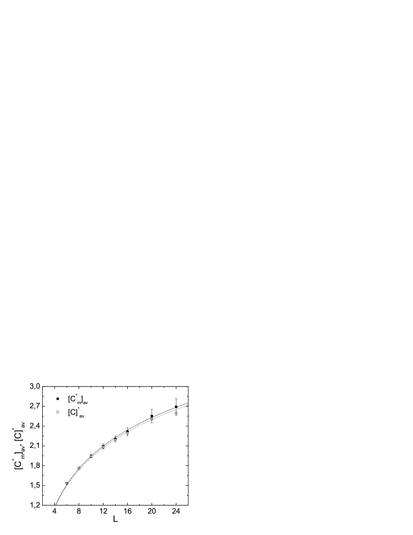
Figure 2: Finite-size behavior of $[C_{m}^{\ast}]_{av}$ and $[C]_{av}^{\ast}$ for $\Delta=0.5$. The solid and dotted lines correspond to logarithmic fits for $[C_{m}^{\ast}]_{av}$ and $[C]_{av}^{\ast}$, respectively.

There are several cases in the literature where the characterization of a phase transition demands very large linear sizes and the picture obtained from moderate sizes is completely misleading. A characteristic example is the 5-state 2D Potts model, for which Landau landa90 suggested that the expected first-order behavior would not be clarified from finite-size data up to sizes $L=2000$. In a different inquiry Hilfer et al. hilfer03 estimated that the asymptotic behavior of the tail regime of the universal order-parameter distribution for the 2D Ising model would require sizes of the order of $L\geq 10^{5}$. Thus, having to deal with the controversial 3D RFIM, for which even the existence a tricritical point at high fields is not yet clarified eich96 , we prefer to regard the observed in figure 1 strong violation of the self-averaging property as a rather tentative conclusion which has to be further verified by studying larger systems and more physical properties (such as the magnetic susceptibility fytas06b ).

Since all past finite temperature studies were attempted on small and moderate sizes ($L\leq 20$), it is valuable to examine the implications of the strong violation of the self-averaging property at these moderate sizes. In our opinion the inconsistent estimations in the literature have, at least partly, their origin on such an unconventional behavior of the RFIM. In order, to observe better these implications we proceed to study, in addition to the above scaling laws, the sample averages of the individual specific heat maxima and pseudocritical temperatures defined by:

$$[C_{m}^{\ast}]_{av} \equiv\frac{1}{M}\sum_{m}C_{m}^{\ast}\cong\widetilde{p}+\widetilde{c}L^{\widetilde{\alpha}/\widetilde{\nu}};$$ (12)

$$[T_{L,m}^{\ast}]_{av} \equiv\frac{1}{M}\sum_{m}T_{L,m}^{\ast}\cong\widetilde{T}_{c}+\widetilde{b}L^{-1/\widetilde{\nu}}.$$

The mean values defined above characterize the corresponding probability distributions and consist a different kind of representative of the samples of RF’s. To quantify the sample-to-sample variations of the specific heat peaks we use the standard deviation of $C_{m}^{\ast}$ over a sample of $m=1,2,...,M$ RF realizations, $V_{C_{m}^{\ast}}$. This is the parameter of equation (11) and figure 1 and will be also illustrated in the following figures as error bars. However, it should not be in any case confused with the statistical errors resulting from the thermal average approximations of equations (2.3) and (7).

3.2 Scaling behavior of the specific heat

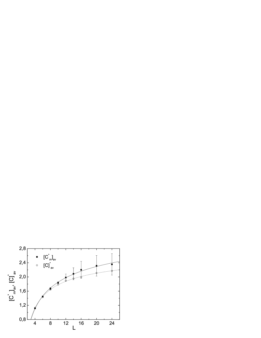
Figure 3: Finite-size behavior of $[C_{m}^{\ast}]_{av}$ and $[C]_{av}^{\ast}$ for $\Delta=1$. The solid and dotted lines correspond to power law fits for $[C_{m}^{\ast}]_{av}$ and $[C]_{av}^{\ast}$, respectively. Both quantities saturate, however with different exponents.

Let us start by presenting in figure 2 the finite-size behavior of the peaks of the sample average $[C_{m}^{\ast}]_{av}$ and that of the averaged curve $[C]_{av}^{\ast}$, for the case $\Delta=0.5$. The number of RF realizations is $M=1000$ for $L\leq 10$ and $M=400$ for $L=12-24$. The difference between the behavior of the peaks of the averaged curve $[C]_{av}^{\ast}$ and that of the sample average $[C_{m}^{\ast}]_{av}$ does not emerge for small values of the lattice size $L$. Only for $L>16$ is the sample-to-sample fluctuation considerable and seems to differentiate, although mildly, between the two averages. Noteworthy that, in this case the standard deviation of the sample-to-sample fluctuations is significantly smaller than the average $[C_{m}^{\ast}]_{av}$: $V_{C_{m}^{\ast}}\ll[C]_{av}^{\ast}<[C_{m}^{\ast}]_{av}$. Based on the data $L=6-24$, no sign of saturation for both $[C_{m}^{\ast}]_{av}$ and $[C]_{av}^{\ast}$ is observed, and one would be tempted to predict a mildly diverging behavior. In fact the best fits, corresponding to the smallest value of $\chi^{2}$ per degree of freedom, predict a logarithmic behavior of the form $[C_{m}^{\ast}]_{av}=0.844(3)\cdot\ln L$ and $[C]_{av}^{\ast}=0.834(4)\cdot\ln L$, respectively. Note that, the fit for $[C_{m}^{\ast}]_{av}$ has a smaller value of $\chi^{2}$ per degree of freedom than that of the fit for $[C]_{av}^{\ast}$. Attempting a power law for $[C_{m}^{\ast}]_{av}$ we find a diverging behavior with a much larger value of $\chi^{2}$ per degree of freedom.

Next, we consider the intermediate case where the randomness takes the value $\Delta=1$. Figure 3 shows again the finite-size behavior of the peaks of the sample average $[C_{m}^{\ast}]_{av}$ and that of the averaged curve $[C]_{av}^{\ast}$. In this case we apply power law fits of the form: $[C]_{av}^{\ast}=p+cL^{w}$ and $[C_{m}^{\ast}]_{av}=\widetilde{p}+\widetilde{c}L^{\widetilde{w}}$, as the one proposed in equations (10) and (12), using the same number of RF realizations as in the case $\Delta=0.5$. These fits yield saturation laws for both cases $[C_{m}^{\ast}]_{av}$ and $[C]_{av}^{\ast}$, predicting however different saturation values $4.15(65)$ and $2.88(13)$, respectively. Specifically, the relevant fits of comparable $\chi^{2}$ quantity, give: $(\widetilde{p},\widetilde{c},\widetilde{w})=(4.15(65),-4.68(44),-0.31(9))$ and $(p,c,w)=(2.88(13),-3.56(64),-0.51(56))$. From these, we could even speculate that the saturation of both quantities takes place with different exponents: $\widetilde{w}=-0.31$ and $w=-0.51$. This value of $w$ corresponding to the peaks of the averaged curve $[C]_{av}^{\ast}$ compares very well to the value $-0.5$ of Ref. rieger93 for the ratio $h/T=0.25$ of their study ($h$ is used for the disorder strength in Ref. rieger93 ). Using our approximate phase diagram (see below figure 6), we find that their case closely corresponds to the case $\Delta=1$ studied here. However, the values of the exponents estimated from the fits can not be taken seriously, since this analysis does not account for the systematic problem that at least part of the data are not yet in the regime of large enough $L$, where finite-size scaling without corrections holds. Note that, the standard deviation of the sample-to-sample fluctuations in this case is also smaller than $[C_{m}^{\ast}]_{av}$, that is $V_{C_{m}^{\ast}}<[C]_{av}^{\ast}<[C_{m}^{\ast}]_{av}$, but not as small as in the case $\Delta=0.5$.

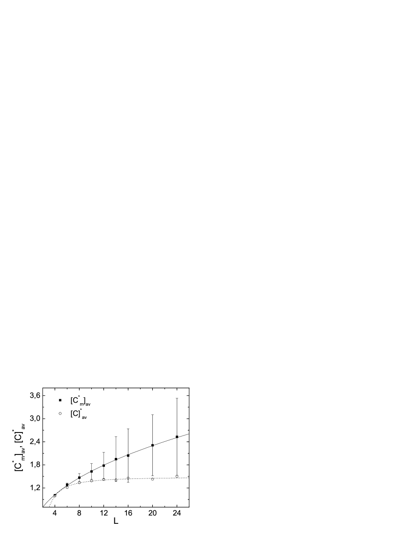
Figure 4: The same as in figure 3, but for $\Delta=1.5$. The clear and early saturation of $[C]_{av}^{\ast}$ is similar to that of the case $\Delta=2$ fytas06a . The diverging power law behavior of $[C_{m}^{\ast}]_{av}$ shown by the solid line gives an exponent $\widetilde{w}=0.44(7)$.

Finally we treat the case $\Delta=1.5$. Figure 4 illustrates the finite-size behavior of the peaks of the sample average $[C_{m}^{\ast}]_{av}$ and that of the averaged curve $[C]_{av}^{\ast}$. The data presented here are taken from samples of $M=1000$ RF’s for $L\leq 12$ and $M=300$ for $L=14-24$. The saturation of the peaks for the averaged curve is quite obvious and is attained, as in the case $\Delta=2$ fytas06a , already in the small $L$-regime. Furthermore, the behavior of the average $[C_{m}^{\ast}]_{av}$ looks similar with that of the case $\Delta=2$ for $L\leq 24$, and despite the fact that there are no signs of saturation of this quantity for these lattice sizes, the possibility of crossing over to a final saturation for larger lattice sizes can not be excluded. It is worth noting that, as in the case $\Delta=2$, the standard deviation of the sample-to-sample fluctuations seems to obey the same behavior with that of $[C_{m}^{\ast}]_{av}$, since $V_{C_{m}^{\ast}}\sim 2([C_{m}^{\ast}]_{av}-[C]_{av}^{\ast})$ and $[C]_{av}^{\ast}\simeq 1.48$. Our power law fitting attempts predict for $[C_{m}^{\ast}]_{av}$ a diverging behavior with $\widetilde{p}=-0.21(3)$, $\widetilde{c}=0.7(2)$, and $\widetilde{w}=0.44(7)$. Meanwhile, the averaged curve $[C]_{av}^{\ast}$ strongly saturates with $p=1.48(2)$, $c=-5.15(1.6)$ and an exponent $w=-1.69(24)$, already from the small $L$-regime. The saturation exponent of the averaged curve $w=\alpha/\nu=-1.69(24)$ should be compared to the value $w=\alpha/\nu=-1.1(4)$ given in Ref. rieger93 for $h/T=0.5$, which now corresponds approximately to our $\Delta=1.5$ case (see figure 6).

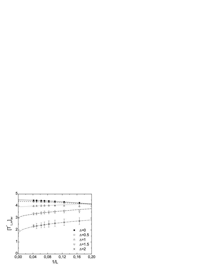
Figure 5: Size dependence of pseudocritical temperatures for various values of $\Delta$, including the case $\Delta=0$ of the normal cubic Ising model malak04 , and the case $\Delta=2$ fytas06a .

Comparing the behavior of $[C_{m}^{\ast}]_{av}$ for the cases $\Delta=1$ and $\Delta=1.5$, one may discern a conflicting picture, in a sense that while $\widetilde{w}$ is negative for $\Delta=1$ - indicating a strong saturation - the same exponent turns out to be positive - indicating a rather strong divergence - for $\Delta=1.5$. We believe though, that this is not a surprise. In fact, the blowing up of the property of lack of self-averaging in the range $\Delta=1-1.5$, as illustrated in the inset of figure 1, may be behind this behavior. A possible saturation in the asymptotic limit may occur in both cases but this may happen via different complex routes because of the unsettled and $(\Delta,L)$-sensitive self-averaging property of the system. On the other hand, the quantity $[C]_{av}^{\ast}$ is very weakly $L$-depended in the large $L$-regime and its early saturation to a value (that depends on the disorder strength), leaves no room for an accurate estimation of its behavior since the statistical errors dominate in the large $L$-regime. This fact, when combined with the possible crossover behavior of the system at quite large linear sizes, larger than those corresponding to the above discussed saturation, lead us to suggest that scaling attempts on $[C]_{av}^{\ast}$, including previous studies, should not be trusted.

3.3 Phase diagram and universality aspects

In figure 5 we present the size dependence of the pseudocritical temperatures for all values of randomness studied. We have included the case of the normal cubic Ising model, for which the numerical data of Ref. malak04 have been used, and the case $\Delta=2$ fytas06a , using results up to $L=24$, where our numerical scheme is accurate. The results of the power law fittings applied (see equation (12)) are presented in table 1. From table 1 it is obvious that there is a strong dependence of the shift exponent ($1/\widetilde{\nu}$) on the value of the disorder strength. While, for relatively small values of the disorder strength $\Delta$ the shifting of the pseudocritical temperatures follows that of the normal Ising model, for larger values of $\Delta$ the exponent $\widetilde{\nu}$ shows an intense variation, indicating a possible violation of universality, in agreement with the results of Sourlas sourlas99 . In fact, it is known that the only theoretical arguments supporting the existence of universality classes in random systems are based on PRG theory and these arguments have been intensively called into questioned for the case of the RFIM. Equivalent studies of universality violations have been reported also in other glassy systems bern96 , reenforcing the view that the concept of universality in complex systems is not fully clarified and that more work needs to be done towards this direction.

Table 1: Critical temperatures and exponents for various values of $\Delta$, including the case $\Delta=0$ of the pure Ising model malak04 , and the case $\Delta=2$ fytas06a .

$\Delta$	$\widetilde{T_{c}}$	$\widetilde{b}$	$\widetilde{\nu}$
0	4.51153	-3.96(14)	0.66(6)
0.5	4.380(3)	-4.12(51)	0.57(24)
1	3.949(19)	1.40(83)	0.95(28)
1.5	3.001(13)	1.85(48)	1.86(34)
2	1.63(19)	2.28(8)	2.55(49)

Based on the data of table 1, we give in figure 6 an approximation of the phase diagram of the model which is comparable with the ones given in the literature (see i.e. Refs. newman96 ; itakura01 ). The dotted line shows a power law fit of the form:

$$T_{c}=p+q\Delta^{r},$$ (13)

with $p=4.5114(20)$, $q=-0.59(3)$, and $r=2.29(6)$. The value of $p$ is very close to the value of the critical temperature of the normal 3D Ising model ($T_{c}\approx 4.51153...$), approving to a certain extent our fitting choice. The above power law ansantz for the phase diagram $T_{c}=T_{c}(\Delta)$ has a clear physical motivation, which could be compared with various functions considered in the past newman96 ; machta00 . The critical value of the randomness is estimated to be $\Delta_{c}=2.42\pm 0.18$, close to the value $2.3\pm 0.2$ of Newman and Barkema newman96 and the value $2.35$ of Ogielski ogielski86 . To get a better estimate for $\Delta_{c}$ the system should be simulated for larger values of $\Delta$ close enough to the critical value.

4 Concluding remarks

The numerical route utilized here for the study of the RFIM consisted of the application of the multi-range WL algorithm wang01 in its N-fold version schul01 , implemented within the CrMES scheme malak04 . We hope that the presented combination of algorithms and techniques will be useful in further numerical studies of this and other similarly challenging problems, such as spin glasses.

Figure 6: The phase diagram based on the data of table 1 and equation (13). The dotted line separates the ferromagnetic (F) from the paramagnetic (P) phase. The estimated critical value $\Delta_{c}$ of the disorder strength, above which no phase transition occurs, is $\Delta_{c}=2.42\pm 0.12$.

Our analysis showed that, in general, the behavior of the mean $[C_{m}^{\ast}]_{av}$ is distinct from that of $[C]_{av}^{\ast}$ and that this is a result of the lack of self-averaging, a property that varies strongly with the disorder strength and the lattice sizes considered. For sufficiently small values of randomness $\Delta$, $[C_{m}^{\ast}]_{av}$ and $[C]_{av}^{\ast}$ seem to obey a mildly diverging behavior, showing no signs of saturation. Moving to the intermediate range $(\Delta=1)$, both quantities saturate, but with different exponents. Yet, this area of the phase diagram of the RFIM is not fully understood. Theoretical studies based on the replica formalism predict the existence of an intermediate glassy-like phase which is characterized by a breaking of replica symmetry near the transition temperature belang98 . However, the interpretation of these results is not clear, and understanding may be simpler under the prism of a strong and complex variation of the property of lack of self-averaging. For large values of randomness, say $\Delta=1.5$, the peak of the averaged specific heat curve $[C]_{av}^{\ast}$ obeys a strong saturation law which is attained already in the small $L$-regime, in agreement with our previous findings for an even larger value of the disorder strength (case $\Delta=2$ fytas06a ). But as mentioned earlier the corresponding scaling attempts would be hardly trusted. In the same range of the disorder strength, the behavior of the sample mean $[C_{m}^{\ast}]_{av}$ is somewhat surprising, showing no signs of saturation, and its behavior seems to follow the large sample-to-sample fluctuations developed by the blowing up of the property of the lack of self-averaging. Apparently, the blowing up of the property of lack of self-averaging in the case $\Delta=1.5$ is responsible for this behavior, shifting a possible saturation to larger values of $L$. Provided that our previous analysis for the case $\Delta=2$ fytas06a recorded a ‘final and unexpected’ saturating behavior of the sample average $[C_{m}^{\ast}]_{av}$ for $L>32$, it will be interesting to observe whether this behavior prevails for larger lattice sizes, even in cases of small values of randomness.

Turning to the shift behavior of the pseudocritical temperatures of the model, we found a very strong dependence of the shift exponent on the disorder strength, reinforcing the scenario of universality violation. The shift for small values of $\Delta$ appears to follow the direction of the pure case $(\Delta=0)$ of shifting to $T_{c}(\Delta)$ from below and this is reflected in the negative sign of the parameter $\widetilde{b}$. For large values of $\Delta$, the power law exponent $\widetilde{\nu}$ shows a very strong variation, which may be due to the existence of additional leading and non-leading correction terms sourlas99 . In order to support numerically the concept of universality for the exponent $\widetilde{\nu}$ one should have accurate data for very large lattices, as has been pointed out also in previous works dealing with the concept of universality in random systems sourlas99 . In conclusion, we argue that the complexity of the self-averaging property for the RFIM may be the main source behind most controversies, and we therefore call attention to the need for studying larger systems.

- (1) Y. Imry, S.-K. Ma, Phys. Rev. Lett. 35, 1399 (1975)
- (2) T. Nattermann, J. Villain, in Phase Transitions 11, 5 (1988)
- (3) D.P. Belanger, A.P. Young, J. Magn. Magn. Mater. 100, 272 (1991)
- (4) H. Rieger, Annual Reviews of Computational Physics II, edited by D. Stauffer (Singapore: World Scientific, 1995)
- (5) D.P. Belanger, T. Nattermann, in Spin Glasses and Random Fields, edited by A.P. Young (Singapore: World Scientific, 1998)
- (6) A.K. Hartmann, A.P. Young, Phys. Rev. B 64, 214419 (2001)
- (7) A.K. Hartmann, U. Nowak, Eur. Phys. J. B 7, 105 (1999)
- (8) M.E.J. Newman, G.T. Barkema, Phys. Rev. E 53, 393 (1996)
- (9) N. Sourlas, Comput. Phys. Commun. 121, 183 (1999)
- (10) G. Parisi, N. Sourlas, Phys. Rev. Lett. 43, 744 (1979)
- (11) G. Grinstein, S.-K. Ma, Phys. Rev. Lett. 49, 685 (1982); Phys. Rev. B 28, 2588 (1983)
- (12) J.Z. Imbrie, Phys. Rev. Lett. 53, 1747 (1984)
- (13) J. Bricmont, A. Kupiainen, Phys. Rev. Lett. 59, 1829 (1987)
- (14) H. Rieger, Phys. Rev. B 52, 6659 (1995)
- (15) J. Villain, J. Phys. Lett. (Paris) 46, 1843 (1985)
- (16) D.S. Fisher, Phys. Rev. Lett. 56, 416 (1985)
- (17) A.J. Bray, M.A. Moore, J. Phys. C 18, 927 (1985)
- (18) A.T. Ogielski, D.A. Huse, Phys. Rev. Lett. 56, 1298 (1986)
- (19) A.T. Ogielski, Phys. Rev. Lett. 57, 1251 (1986)
- (20) S.R. McCay, A.N. Berker, J. Appl. Phys. 64, 5785 (1988)
- (21) A. Aharony, Phys. Rev. B 18, 3318 (1978)
- (22) J.T. Chayes, L. Chayes, D.S. Fisher, T. Spencer, Phys. Rev. Lett. 57, 2999 (1986)
- (23) J. Cardy, Scaling and Renormalization in Statistical Physics (Cambridge University Press, Cambridge, 1996)
- (24) A.B. Harris, J. Phys. C 7, 1671 (1976)
- (25) M. Itakura, Phys. Rev. B 64, 012415 (2001)
- (26) M. Mézard, A.P. Young, Europhys. Lett. 18, 653 (1992)
- (27) M. Mézard, R. Monasson, Phys. Rev. B 50, 7199 (1994)
- (28) J-C. Anglés d’ Auriac, N. Sourlas, Europhys. Lett. 39, 473 (1997)
- (29) A. Malakis, N.G. Fytas, Phys. Rev. E 73, 016109 (2006)
- (30) N.G. Fytas, A. Malakis, Eur. Phys. J. B (to be published)
- (31) H. Rieger, A.P. Young, J. Phys. A 26, 5279 (1993)
- (32) U. Nowak, K.D. Usadel, J. Esser, Physica A 250, 1 (1998)
- (33) A.A. Middleton, D.S. Fisher, Phys. Rev. B 65, 134411 (2002)
- (34) S. Fishman, A. Aharony, J. Phys. C 12, 729 (1979)
- (35) J. Cardy, Phys. Rev. B 29, 505 (1985)
- (36) D.P. Belanger, A.R. King, V. Jaccarino, J.L. Cardy, Phys. Rev. B 28, 2522 (1983)
- (37) M. Hagen, R.A. Cowley, S.K. Satija, H. Yoshizawa, G. Shirane, R.J. Birgeneau, H.J. Guggenheim, Phys. Rev. B 28, 2602 (1983)
- (38) D.P. Belanger, A.R. King, V. Jaccarino, Phys. Rev. B 31, 4538 (1985); P. Pollack, W. Kleeman, D.P. Belanger, Phys. Rev. B 38, 4773 (1988)
- (39) W.C. Barber, D.P. Belanger, J. Magn. Magn. Mater. 226, 545 (2001)
- (40) M. Karszewiski, J. Kushauer, Ch. Binek, W. Kleeman, D. Bertrand, J. Phys. C 6, 75 (1994)
- (41) G. Grinstein, Phys. Rev. Lett. 37, 944 (1976)
- (42) A. Malakis, A. Peratzakis, N.G. Fytas, Phys. Rev. E 70, 066128 (2004); A. Malakis, S.S. Martinos, I.A. Hadjiagapiou, N.G. Fytas, P. Kalozoumis, Phys. Rev. E 72, 066120 (2005)
- (43) N. Metropolis, A. Rosenbluth, M. Rosenbluth, A. Teller, E. Teller, J. Chem. Phys. 21, 1087 (1953)
- (44) M.E.J. Newman, G.T. Barkema, Monte Carlo Methods in Statistical Physics (Oxford: Clarendon Press, 1999)
- (45) A.P. Young, M. Nauenburg, Phys. Rev. Lett. 54, 2429 (1986)
- (46) I. Dukovski, J. Machta, Phys. Rev. B 67, 014413 (2003)
- (47) N.M.S. Swamy, K. Thulasiraman, Graphs, Networks and Algorithms (New York: Wiley, 1990)
- (48) Y. Wu, J. Machta, Phys. Rev. Lett. 95, 137208 (2005)
- (49) V.S. Dotsenko, W. Selke, A.L. Talapov, Physica A 170, 278 (1991)
- (50) U. Wolff, Phys. Rev. Lett. 62, 361 (1989)
- (51) A.M. Ferrenberg, R.H Swendsen, Phys. Rev. Lett. 61, 2635 (1988); Phys. Rev. Lett. 63, 1195 (1989)
- (52) R.H. Swendsen, J.-S. Wang, Phys. Rev. Lett. 57, 2607 (1986)
- (53) O. Redner, J. Machta, L.F. Chayes, Phys. Rev. E 58, 2749 (1998); L. Chayes, J. Machta, O. Redner, J. Stat. Phys. 93, 17 (1998)
- (54) J. Machta, M.E.J. Newman, L.B. Chayes, Phys. Rev. E 62, 8782 (2000)
- (55) A. Malakis, S.S. Martinos, I.A. Hadjiagapiou, A.S. Peratzakis, Int. J. Mod. Phys. C 15, 729 (2004)
- (56) J. Lee, Phys. Rev. Lett. 71, 211 (1993)
- (57) B.A. Berg, T. Neuhaus, Phys. Rev. Lett. 68, 9 (1992)
- (58) A.R. Lima, P.M.C. de Oliveira, T.J.P. Penna, J. Stat. Phys. 99, 961 (2000)
- (59) F. Wang, D.P. Landau, Phys. Rev. Lett. 86, 2050 (2001); Phys. Rev. E 64, 056101 (2001); D.P. Landau, F. Wang, Comput. Phys. Commun. 147, 674 (2002)
- (60) B.J. Schulz, K. Binder, M. Muller, Int. J. Mod. Phys. C 13, 477 (2001)
- (61) P.M.C. de Oliveira, T.J.P. Penna, H.J. Herrmann, Braz. J. Phys. 26, 677 (1996)
- (62) C. Zhou, R.N. Bhatt, Phys. Rev. E 72, 025701(R) (2005)
- (63) G. Parisi, N. Sourlas, Phys. Rev. Lett. 89, 257204 (2002)
- (64) K. Binder, D.W. Heermann, Monte Carlo Simulations in Statistical Physics (Berlin: Springer-Verlag, 1988)
- (65) S. Wiseman, E. Domany, Phys. Rev. E 52, 3469 (1995); Phys. Rev. Lett. 81, 22 (1998)
- (66) A. Aharony, A.B. Harris, Phys. Rev. Lett. 77, 3700 (1996)
- (67) D.P. Landau, in Finite Size Scaling and Numerical Simulations of Statistical systems, edited by V. Privman (Singapore: World Scientific, 1990)
- (68) R. Hilfer, B. Biswal, H.G. Mattutis, W. Janke, Phys. Rev. E 68, 046123 (2003)
- (69) K. Eichhorn, K. Binder, J. Phys. C 8, 5209 (1996)
- (70) L.W. Bernard, S. Prakash, I.A. Campbell, Phys. Rev. Lett. 77, 2798 (1996)