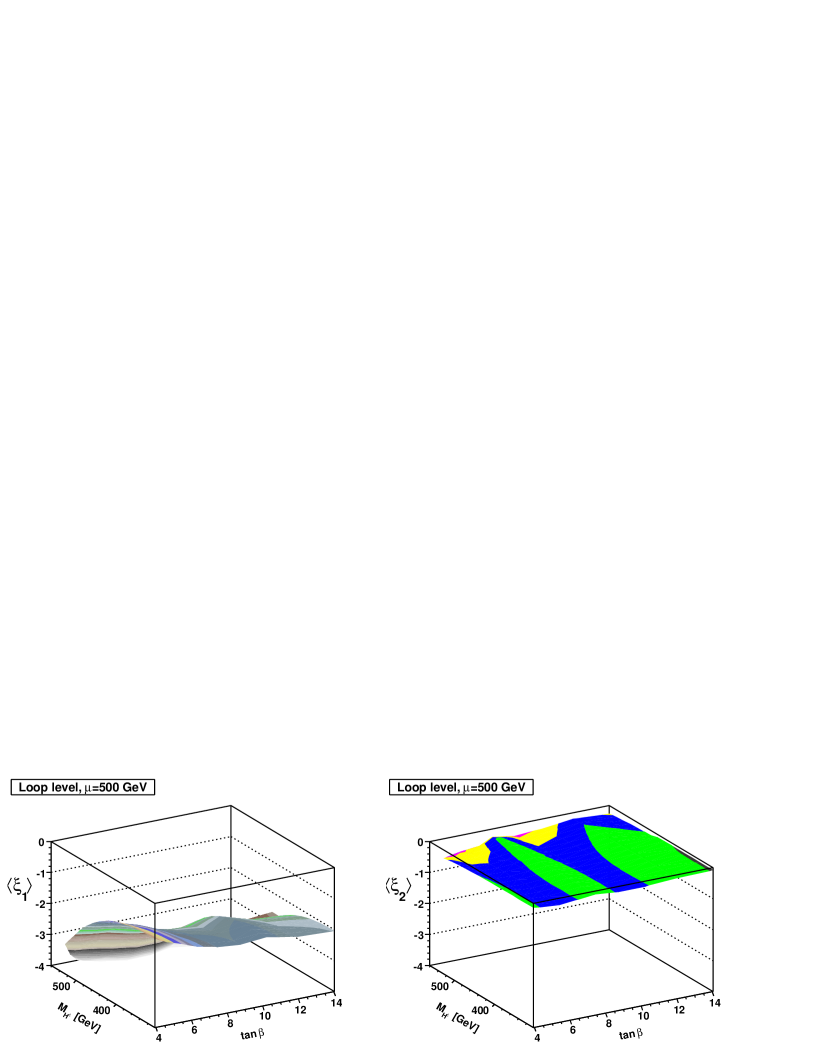
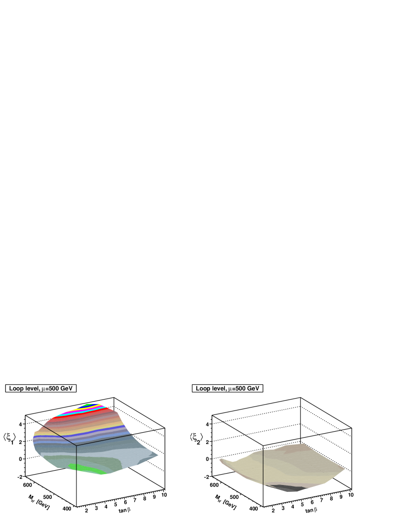
Trilinear Higgs couplings in the two Higgs doublet model with CP violation

Per Osland per.osland@ift.uib.no Department of Physics and Technology, University of Bergen, Postboks 7803, N-5020 Bergen, Norway    P. N. Pandita ppandita@nehu.ac.in Service de Physique Théorique, CEA-Saclay, F-91191 Gif-sur-Yvette Cedex, France and
Department of Physics, North Eastern Hill University, Shillong 793 022, India111Permanent address
   Levent Selbuz Levent.Selbuz@eng.ankara.edu.tr Department of Physics and Technology, University of Bergen, Postboks 7803, N-5020 Bergen, Norway and
Department of Engineering Physics, Faculty of Engineering, Ankara University, 06100 Tandogan-Ankara, Turkey222Permanent address
Abstract

We carry out a detailed analysis of the general two Higgs doublet model with CP violation. We describe two different parametrizations of this model, and then study the Higgs boson masses and the trilinear Higgs couplings for these two parametrizations. Within a rather general model, we find that the trilinear Higgs couplings have a significant dependence on the details of the model, even when the lightest Higgs boson mass is taken to be a fixed parameter. We include radiative corrections in the one-loop effective potential approximation in our analysis of the Higgs boson masses and the Higgs trilinear couplings. The one-loop corrections to the trilinear couplings of the two Higgs doublet model also depend significantly on the details of the model, and can be rather large. We study quantitatively the trilinear Higgs couplings, and show that these couplings are typically several times larger than the corresponding Standard Model trilinear Higgs coupling in some regions of the parameter space. We also briefly discuss the decoupling limit of the two Higgs doublet model.

Two Higgs doublet model, trilinear couplings, CP violation
pacs:
12.60.Fr, 14.80.Cp, 11.30.Er

I Introduction

The Higgs mechanism Englert:1964et of spontaneous electroweak symmetry breaking is a necessary ingredient of the Standard Model (SM), which is crucial for its internal consistency. The search for the Higgs boson is, thus, one of the major tasks for the experiments at the upcoming Large Hadron Collider (LHC). In order to confirm the Higgs mechanism as the origin of spontaneous breaking of SU(2)L×U(1)Y𝑆𝑈subscript2𝐿𝑈subscript1𝑌SU(2)_{L}\times U(1)_{Y} gauge symmetry in the SM, not only must the Higgs boson be discovered, but also its trilinear (λHHHSMsuperscriptsubscript𝜆𝐻𝐻𝐻SM\lambda_{HHH}^{\text{SM}}) and quartic (λHHHHSMsuperscriptsubscript𝜆𝐻𝐻𝐻𝐻SM\lambda_{HHHH}^{\text{SM}}) self couplings must be measured in order to completely reconstruct the Higgs potential. Furthermore, one must also be able to measure the couplings of the Higgs boson to gauge bosons and fermions.

Here we shall be concerned mainly with the trilinear self couplings of the Higgs boson. In the Standard Model, there is only one trilinear self coupling of the Higgs boson which can be written simply in terms of the Higgs boson mass MHsubscript𝑀𝐻M_{H} as

λHHHSM=3MH2v,superscriptsubscript𝜆𝐻𝐻𝐻SM3superscriptsubscript𝑀𝐻2𝑣\lambda_{HHH}^{\text{SM}}=\frac{3M_{H}^{2}}{v}, (1)

where v=2MW/g=246𝑣2subscript𝑀𝑊𝑔246v=2M_{W}/g=246 GeV is the vacuum expectation value of the neutral component of the Higgs doublet, MWsubscript𝑀𝑊M_{W} is the mass of the W±superscript𝑊plus-or-minusW^{\pm}, and g𝑔g is the SU(2)L𝑆𝑈subscript2𝐿SU(2)_{L} gauge coupling, respectively. Several extensions of the SM, such as the minimal supersymmetric standard model (MSSM) Nilles:1983ge , and the general two Higgs doublet model (2HDM) Gunion:1989we , have a more complicated Higgs structure. In these models there are several trilinear Higgs couplings, having more complicated dependence on the underlying masses. It is a challenging task to measure Weiglein:2004hn these trilinear couplings at the LHC. On the other hand a linear collider could possibly offer much better prospects of measuring these trilinear Higgs couplings Accomando:1997wt ; Djouadi:1996ah ; AguilarSaavedra:2001rg ; Arhrib:2008jp ; Ferrera:2007sp .

At the proposed International Linear Collider (ILC), if the Higgs boson is not too heavy, the trilinear Higgs coupling can be measured via the Higgs boson pair production e+eW+ν¯WνHHν¯νsuperscript𝑒superscript𝑒superscript𝑊absent¯𝜈superscript𝑊absent𝜈𝐻𝐻¯𝜈𝜈e^{+}e^{-}\rightarrow W^{+*}\overline{\nu}W^{-*}\nu\to HH\overline{\nu}\nu. A precise measurement of the trilinear Higgs self coupling will also make it possible to test extended Higgs models, which have a different structure of the Higgs potential, and hence different trilinear Higgs couplings, as compared to the SM. The 2HDM is the simplest, yet a very general, model with an extended Higgs structure, which leads to various distinct physical effects. In particular, the model can easily accommodate additional CP violation  Lee:1973iz ; Weinberg:1976hu ; Branco:1985aq ; Accomando:2006ga , beyond what is generated by the Kobayashi–Maskawa (KM) mechanism Cabibbo:yz . Furthermore, since there is a distinct possibility of measuring precisely the Higgs boson self couplings at the ILC, there is a motivation to study the radiative corrections to the trilinear self couplings of the Higgs boson.

On the other hand, there are a number of parameters in the potential of the two Higgs doublet model, including those associated with CP violation, which determine the masses and CP properties of the model. In spite of the complicated nature of the Higgs potential, it has been shown in the 2HDM with CP conservation that one-loop corrections to the lightest CP-even Higgs boson self coupling are in general of a non decoupling nature, and can give rise to 𝒪(100%)𝒪percent100\mathcal{O}(100\%) deviations from the SM prediction Kanemura:2002vm . This happens even when all other couplings of the lightest Higgs boson to gauge bosons and fermions are in good agreement with the SM prediction.

In this paper we shall study in detail the trilinear Higgs couplings in the two Higgs Doublet Model (2HDM) with CP violation. We shall assume that the underlying gauge group is the SM gauge group. After spontaneous breaking of the SM gauge symmetry, the Higgs spectrum of the model consists of three neutral Higgs bosons and two charged Higgs bosons. In the CP-conserving version of the model, two neutral Higgs bosons (h0,H0superscript0superscript𝐻0h^{0},H^{0}) are CP even, whereas one neutral Higgs boson (A0superscript𝐴0A^{0}) is CP odd. In the CP-conserving case, there are, thus, six allowed trilinear Higgs couplings which can be labelled as λhhhsubscript𝜆\lambda_{hhh}, λhhHsubscript𝜆𝐻\lambda_{hhH}, λhHHsubscript𝜆𝐻𝐻\lambda_{hHH}, λHHHsubscript𝜆𝐻𝐻𝐻\lambda_{HHH} involving the CP-even Higgs bosons, and λhAAsubscript𝜆𝐴𝐴\lambda_{hAA}, λHAAsubscript𝜆𝐻𝐴𝐴\lambda_{HAA}, all even in the number of A0superscript𝐴0A^{0}, involving the CP-odd Higgs boson. When CP is not conserved, the neutral Higgs bosons do not have a definite CP, and there is no such constraint on the couplings involving the A0superscript𝐴0A^{0} Higgs boson. There, are, thus, a total of ten trilinear Higgs couplings in the case of the 2HDM with CP violation.

Since this is one of the simplest models which goes beyond the KM mechanism of CP violation, it is important to study the impact of CP violation on the Higgs self couplings in this model. We shall, therefore, consider the 2HDM with explicit CP violation in the Higgs sector in this paper. This explicit CP violation is introduced through appropriate complex parameters in the potential of the 2HDM. Furthermore, we shall assume that this explicit CP violation cannot be transformed away by a redefinition of the Higgs fields. Thus, one of the objectives of the present study is to determine the effects of this explicit CP violation in the Higgs sector on various Higgs self couplings in the two Higgs doublet model. In our study of the model, we shall find it convenient to keep the masses of the two lightest neutral Higgs bosons fixed, and then study the dependence on other parameters of the model, which will determine the amount of explicit CP violation in various Higgs self couplings, and also determine the mass of the heaviest Higgs boson. In this way, we do not lay emphasis on the heavy Higgs sector of the theory, whereas at the same time we can exhibit the wide range of values that the trilinear Higgs couplings can assume. In particular, we wish to emphasize that, in contrast to the MSSM, the heavy mass effects in a general 2HDM do not decouple. In order to demonstrate this we shall calculate the one-loop corrected Higgs boson self-couplings using the method of effective potential in a general 2HDM with explicit CP violation as described above. This is in contrast to Ref. Kanemura:2002vm , where all couplings and mass parameters were assumed to be real, thereby precluding the phenomena of explicit CP violation in the Higgs sector as considered in this paper.

The plan of this paper is as follows. In Section II we describe the most general two Higgs doublet model with CP violation. We then discuss the spectrum of the Higgs bosons of the model, and the constraints on the parameters when there is CP violation in the model. Here we also discuss how only certain sets of parameters of the Higgs potential can lead to physically consistent models, and discuss different ways in which these parameters can be specified. We delineate the regions of the parameter space where there is no CP violation, corresponding to which one of the neutral Higgs bosons is odd under P. In Section III we derive the tree level trilinear couplings between the neutral as well as the charged Higgs bosons of the model, and discuss the correspondence of these couplings with the trilinear Higgs couplings of the minimal supersymmetric standard model. Here we also study numerically the trilinear Higgs couplings, and discuss the domain of the parameter space that is compatible with various theoretical and experimental constraints.

In Section IV we use the method of one-loop effective potential to calculate, as a first step, one-loop corrections to the Higgs boson masses. In Section V, we then calculate the one-loop corrections to the trilinear self couplings of the Higgs bosons. In Section VI we carry out a detailed numerical study of the one-loop corrected trilinear Higgs couplings, discuss the magnitudes of different contributions, the dependence on the scale, as well as the decoupling limit, and show that these couplings can be several times larger than the corresponding Standard Model trilinear Higgs coupling in some regions of the parameter space. We summarize our results and conclusions in Section VII. Some of the analytical calculations used in our analysis are described in appendices.

II The Two-Higgs-Doublet Model

The general 2HDM with the underlying gauge group SU(2)L×U(1)Y𝑆𝑈subscript2𝐿𝑈subscript1𝑌SU(2)_{L}\times U(1)_{Y} is obtained by extending the Higgs sector of the SM with a second SU(2)L𝑆𝑈subscript2𝐿SU(2)_{L} Higgs doublet with weak hypercharge Y=1.𝑌1Y=1. Thus, the model contains 444 complex scalar fields which are arranged as SU(2)L𝑆𝑈subscript2𝐿SU(2)_{L} doublets as follows:

Φi=(φi+φi0)(Y=+1),i=1, 2.formulae-sequencesubscriptΦ𝑖matrixsuperscriptsubscript𝜑𝑖superscriptsubscript𝜑𝑖0𝑌1𝑖12\Phi_{i}=\begin{pmatrix}\varphi_{i}^{+}\\ \varphi_{i}^{0}\end{pmatrix}\quad(Y=+1),\quad i=1,\,2. (2)

Using these two Higgs doublets, the most general renormalizable potential for the 2HDM which is invariant under the SU(2)L×U(1)Y𝑆𝑈subscript2𝐿𝑈subscript1𝑌SU(2)_{L}\times U(1)_{Y} gauge group can be written as

Vtreesubscript𝑉tree\displaystyle V_{\text{tree}} =λ12(Φ1Φ1)2+λ22(Φ2Φ2)2+λ3(Φ1Φ1)(Φ2Φ2)absentsubscript𝜆12superscriptsuperscriptsubscriptΦ1subscriptΦ12subscript𝜆22superscriptsuperscriptsubscriptΦ2subscriptΦ22subscript𝜆3superscriptsubscriptΦ1subscriptΦ1superscriptsubscriptΦ2subscriptΦ2\displaystyle=\frac{\lambda_{1}}{2}(\Phi_{1}^{\dagger}\Phi_{1})^{2}+\frac{\lambda_{2}}{2}(\Phi_{2}^{\dagger}\Phi_{2})^{2}+\lambda_{3}(\Phi_{1}^{\dagger}\Phi_{1})(\Phi_{2}^{\dagger}\Phi_{2})
+λ4(Φ1Φ2)(Φ2Φ1)+12[λ5(Φ1Φ2)2+h.c.]\displaystyle+\lambda_{4}(\Phi_{1}^{\dagger}\Phi_{2})(\Phi_{2}^{\dagger}\Phi_{1})+\frac{1}{2}\left[\lambda_{5}(\Phi_{1}^{\dagger}\Phi_{2})^{2}+{\rm h.c.}\right]
+{[λ6(Φ1Φ1)+λ7(Φ2Φ2)](Φ1Φ2)+h.c.}\displaystyle+\left\{\left[\lambda_{6}(\Phi_{1}^{\dagger}\Phi_{1})+\lambda_{7}(\Phi_{2}^{\dagger}\Phi_{2})\right](\Phi_{1}^{\dagger}\Phi_{2})+{\rm h.c.}\right\}
12{m112(Φ1Φ1)+[m122(Φ1Φ2)+h.c.]\displaystyle-\frac{1}{2}\bigl{\{}m_{11}^{2}(\Phi_{1}^{\dagger}\Phi_{1})+\left[m_{12}^{2}(\Phi_{1}^{\dagger}\Phi_{2})+{\rm h.c.}\right]
+m222(Φ2Φ2)},\displaystyle+m_{22}^{2}(\Phi_{2}^{\dagger}\Phi_{2})\bigr{\}}, (3)

where λi(i=1,,7)subscript𝜆𝑖𝑖17\lambda_{i}~{}(i=1,\ldots,7) are dimensionless parameters and the subscript “tree” denotes that (3) is a tree-level potential. We note that λi(i=1,,4)subscript𝜆𝑖𝑖14\lambda_{i}~{}(i=1,\ldots,4) are real, whereas λi(i=5,,7)subscript𝜆𝑖𝑖57\lambda_{i}~{}(i=5,\ldots,7) are in general complex parameters. Similarly, m112subscriptsuperscript𝑚211m^{2}_{11} and m222subscriptsuperscript𝑚222m^{2}_{22} are real, whereas m122subscriptsuperscript𝑚212m^{2}_{12} is in general complex. We note that the terms proportional to λ6subscript𝜆6\lambda_{6} and λ7subscript𝜆7\lambda_{7} have to be constrained, since this potential does not satisfy natural flavor conservation Glashow:1976nt , even when each doublet is coupled only to up-type or only to down-type quarks.

When the neutral components of the two Higgs doublets Φ1,2subscriptΦ12\Phi_{1,2} acquire vacuum expectation values (VEVs), φ1,20=v1,2/2subscriptsuperscript𝜑012subscript𝑣122\varphi^{0}_{1,2}=v_{1,2}/\sqrt{2}, the gauge group SU(2)L×U(1)Y𝑆𝑈subscript2𝐿𝑈subscript1𝑌SU(2)_{L}\times U(1)_{Y} breaks down to U(1)em,𝑈subscript1emU(1)_{\rm em}, whereby three of the eight real fields in (2) are absorbed by three of the four gauge bosons of SU(2)L×U(1)Y,𝑆𝑈subscript2𝐿𝑈subscript1𝑌SU(2)_{L}\times U(1)_{Y}, which become massive in the process, leaving behind a massless photon. We can then parametrize the two Higgs doublet fields in (2) as

Φi=(φi+12(vi+ηi+iχi)),i=1, 2,formulae-sequencesubscriptΦ𝑖matrixsuperscriptsubscript𝜑𝑖12subscript𝑣𝑖subscript𝜂𝑖𝑖subscript𝜒𝑖𝑖12\Phi_{i}=\begin{pmatrix}\varphi_{i}^{+}\\ \frac{1}{\sqrt{2}}(v_{i}+\eta_{i}+i\chi_{i})\end{pmatrix},\quad i=1,\,2, (4)

where we have chosen the VEVs of the neutral Higgs fields to be real, and absorbed the relative phase between the two VEVs in the parameters m122,λ5,λ6subscriptsuperscript𝑚212subscript𝜆5subscript𝜆6m^{2}_{12},\lambda_{5},\lambda_{6} and λ7subscript𝜆7\lambda_{7} of Vtreesubscript𝑉treeV_{\rm tree}. When we substitute the parametrisation (4) of the Higgs fields in the potential (3), there will be cubic terms in the Higgs fields arising from the quartic couplings λisubscript𝜆𝑖\lambda_{i}, which will give rise to trilinear couplings among the Higgs fields. It is these trilinear couplings that we shall study in detail in this paper.

As discussed in the Introduction, in the case of 2HDM with CP conservation, after spontaneous breakdown of the gauge symmetry, we are left with two CP-even Higgs bosons h0,H0,superscript0superscript𝐻0h^{0},H^{0}, a CP-odd Higgs boson A0,superscript𝐴0A^{0}, and a pair of charged Higgs bosons H±superscript𝐻plus-or-minusH^{\pm}. However, with CP violation the neutral Higgs bosons h0,H0,A0superscript0superscript𝐻0superscript𝐴0h^{0},H^{0},A^{0} mix, and it is then more appropriate to define the weak states

(η1η2η3),matrixsubscript𝜂1subscript𝜂2subscript𝜂3\begin{pmatrix}\eta_{1}\\ \eta_{2}\\ \eta_{3}\end{pmatrix}, (5)

to describe the neutral Higgs sector of the CP violating two Higgs doublet model. In (5) we have defined

η3subscript𝜂3\displaystyle\eta_{3} =sinβχ1+cosβχ2,absent𝛽subscript𝜒1𝛽subscript𝜒2\displaystyle=-\sin\beta\,\chi_{1}+\cos\beta\,\chi_{2}, (6)
G0superscript𝐺0\displaystyle G^{0} =cosβχ1+sinβχ2,absent𝛽subscript𝜒1𝛽subscript𝜒2\displaystyle=\cos\beta\,\chi_{1}+\sin\beta\,\chi_{2}, (7)

where G0superscript𝐺0G^{0} is the would-be neutral Goldstone boson, and tanβ=v2/v1𝛽subscript𝑣2subscript𝑣1\tan\beta=v_{2}/v_{1} is the ratio of the vacuum expectation values of the two Higgs fields. We shall take tanβ𝛽\tan\beta as an independent parameter. The charged Higgs fields and the corresponding charged Goldstone boson are likewise defined as

H±superscript𝐻plus-or-minus\displaystyle H^{\pm} =sinβφ1±+cosβφ2±,absent𝛽subscriptsuperscript𝜑plus-or-minus1𝛽subscriptsuperscript𝜑plus-or-minus2\displaystyle=-\sin\beta\,\varphi^{\pm}_{1}+\cos\beta\,\varphi^{\pm}_{2}, (8)
G±superscript𝐺plus-or-minus\displaystyle G^{\pm} =cosβφ1±+sinβφ2±,absent𝛽subscriptsuperscript𝜑plus-or-minus1𝛽subscriptsuperscript𝜑plus-or-minus2\displaystyle=\cos\beta\,\varphi^{\pm}_{1}+\sin\beta\,\varphi^{\pm}_{2}, (9)

respectively.

II.1 Basis rotation

The tree-level mass squared matrix of the neutral Higgs bosons can now be defined as

ij2=2Vηiηj,subscriptsuperscript2𝑖𝑗superscript2𝑉subscript𝜂𝑖subscript𝜂𝑗{\cal M}^{2}_{ij}=\frac{\partial^{2}V}{\partial\eta_{i}\partial\eta_{j}}, (10)

where, after differentiation, all fields are set equal to zero: η1=η2=η3=H±=G0=G±=0subscript𝜂1subscript𝜂2subscript𝜂3superscript𝐻plus-or-minussuperscript𝐺0superscript𝐺plus-or-minus0\eta_{1}=\eta_{2}=\eta_{3}=H^{\pm}=G^{0}=G^{\pm}=0. The physical neutral Higgs states Hisubscript𝐻𝑖H_{i}, which are the eigenstates of the mass squared matrix (10), are then obtained by a rotation R𝑅R

H=Rη,η=RTH,formulae-sequence𝐻𝑅𝜂𝜂superscript𝑅T𝐻H=R\eta,\quad\eta=R^{\text{T}}H, (11)

or, more explicitly

Hi=Rijηj,ηj=RijHi.formulae-sequencesubscript𝐻𝑖subscript𝑅𝑖𝑗subscript𝜂𝑗subscript𝜂𝑗subscript𝑅𝑖𝑗subscript𝐻𝑖H_{i}=R_{ij}\eta_{j},\quad\eta_{j}=R_{ij}H_{i}. (12)

The rotation matrix R𝑅R which diagonalizes (10),

R2RT=diag2=diag(M12,M22,M32),𝑅superscript2superscript𝑅Tsubscriptsuperscript2diagdiagsuperscriptsubscript𝑀12superscriptsubscript𝑀22superscriptsubscript𝑀32R{\cal M}^{2}R^{\rm T}={\cal M}^{2}_{\rm diag}={\rm diag}(M_{1}^{2},M_{2}^{2},M_{3}^{2}), (13)

with M1<M2<M3subscript𝑀1subscript𝑀2subscript𝑀3M_{1}<M_{2}<M_{3}, can be parametrized as

R=R3R2R1=𝑅subscript𝑅3subscript𝑅2subscript𝑅1absent\displaystyle R=R_{3}\,R_{2}\,R_{1}= (1000cosα3sinα30sinα3cosα3)(cosα20sinα2010sinα20cosα2)(cosα1sinα10sinα1cosα10001)matrix1000subscript𝛼3subscript𝛼30subscript𝛼3subscript𝛼3matrixsubscript𝛼20subscript𝛼2010subscript𝛼20subscript𝛼2matrixsubscript𝛼1subscript𝛼10subscript𝛼1subscript𝛼10001\displaystyle\begin{pmatrix}1&0&0\\ 0&\cos\alpha_{3}&\sin\alpha_{3}\\ 0&-\sin\alpha_{3}&\cos\alpha_{3}\end{pmatrix}\begin{pmatrix}\cos\alpha_{2}&0&\sin\alpha_{2}\\ 0&1&0\\ -\sin\alpha_{2}&0&\cos\alpha_{2}\end{pmatrix}\begin{pmatrix}\cos\alpha_{1}&\sin\alpha_{1}&0\\ -\sin\alpha_{1}&\cos\alpha_{1}&0\\ 0&0&1\end{pmatrix}
=\displaystyle= (c1c2s1c2s2(c1s2s3+s1c3)c1c3s1s2s3c2s3c1s2c3+s1s3(c1s3+s1s2c3)c2c3),matrixsubscript𝑐1subscript𝑐2subscript𝑠1subscript𝑐2subscript𝑠2subscript𝑐1subscript𝑠2subscript𝑠3subscript𝑠1subscript𝑐3subscript𝑐1subscript𝑐3subscript𝑠1subscript𝑠2subscript𝑠3subscript𝑐2subscript𝑠3subscript𝑐1subscript𝑠2subscript𝑐3subscript𝑠1subscript𝑠3subscript𝑐1subscript𝑠3subscript𝑠1subscript𝑠2subscript𝑐3subscript𝑐2subscript𝑐3\displaystyle\begin{pmatrix}c_{1}\,c_{2}&s_{1}\,c_{2}&s_{2}\\ -(c_{1}\,s_{2}\,s_{3}+s_{1}\,c_{3})&c_{1}\,c_{3}-s_{1}\,s_{2}\,s_{3}&c_{2}\,s_{3}\\ -c_{1}\,s_{2}\,c_{3}+s_{1}\,s_{3}&-(c_{1}\,s_{3}+s_{1}\,s_{2}\,c_{3})&c_{2}\,c_{3}\end{pmatrix}, (14)

where ci=cosαisubscript𝑐𝑖subscript𝛼𝑖c_{i}=\cos\alpha_{i}, si=sinαisubscript𝑠𝑖subscript𝛼𝑖s_{i}=\sin\alpha_{i}. Note that Eq. (13) can be inverted as

(2)ij=kRkiMk2Rkj.subscriptsuperscript2𝑖𝑗subscript𝑘subscript𝑅𝑘𝑖superscriptsubscript𝑀𝑘2subscript𝑅𝑘𝑗({\cal M}^{2})_{ij}=\sum_{k}R_{ki}M_{k}^{2}R_{kj}. (15)

By symmetry, (2)ji=(2)ijsubscriptsuperscript2𝑗𝑖subscriptsuperscript2𝑖𝑗({\cal M}^{2})_{ji}=({\cal M}^{2})_{ij}, and, in the general case, this matrix is seen to contain 6 independent parameters. These may be taken as the three masses, and the angles of the rotation matrix.

As discussed in Ref. ElKaffas:2007rq , there are three limits in which there is no CP violation in the 2HDM, corresponding to which one of the neutral Higgs bosons is odd under P. These limits can be characterised in terms of the angles α2subscript𝛼2\alpha_{2} and α3subscript𝛼3\alpha_{3} of the rotation matrix (II.1) as follows:

H1 is odd:subscript𝐻1 is odd:\displaystyle H_{1}\text{ is odd:} α2=±π/2,subscript𝛼2plus-or-minus𝜋2\displaystyle\alpha_{2}=\pm\pi/2, (16)
H2 is odd:subscript𝐻2 is odd:\displaystyle H_{2}\text{ is odd:} α3=±π/2,subscript𝛼3plus-or-minus𝜋2\displaystyle\alpha_{3}=\pm\pi/2, (17)
H3 is odd:subscript𝐻3 is odd:\displaystyle H_{3}\text{ is odd:} α2=0,α3=0.formulae-sequencesubscript𝛼20subscript𝛼30\displaystyle\alpha_{2}=0,\ \ \alpha_{3}=0. (18)

We note that in the latter limit, we have α1=α+π/2subscript𝛼1𝛼𝜋2\alpha_{1}=\alpha+\pi/2, where α𝛼\alpha is the conventional mixing angle in the CP-even sector of the MSSM Gunion:1989we . Any CP violation in the 2HDM will also depend on the Yukawa couplings. In the 2HDM II (Model II), where the down-type quarks couple to Φ1subscriptΦ1\Phi_{1} and the up-type quarks couple to Φ2subscriptΦ2\Phi_{2}, various measures of “maximal” CP violation both in the Higgs-vector boson and Higgs-quark sectors are discussed in Khater:2003ym . These maxima occur in the “bulk” of the α2subscript𝛼2\alpha_{2}α3subscript𝛼3\alpha_{3} space, typically for |α2|=𝒪(π/4)subscript𝛼2𝒪𝜋4|\alpha_{2}|={\cal O}(\pi/4) and |α3|=𝒪(π/4)subscript𝛼3𝒪𝜋4|\alpha_{3}|={\cal O}(\pi/4).

II.2 Neutral Higgs boson masses

Minimizing the tree-level potential according to

VΦi=0,i=1, 2,formulae-sequence𝑉subscriptΦ𝑖0𝑖12\frac{\partial V}{\partial\Phi_{i}}=0,\quad i=1,\,2, (19)

and using the resulting minimization conditions to eliminate m112superscriptsubscript𝑚112m_{11}^{2} and m222,superscriptsubscript𝑚222m_{22}^{2}, one obtains the elements (10) of the tree-level mass squared matrix

112subscriptsuperscript211\displaystyle{\cal M}^{2}_{11} =v12λ1+v22ν+v22v1Re(3v12λ6v22λ7),absentsuperscriptsubscript𝑣12subscript𝜆1superscriptsubscript𝑣22𝜈subscript𝑣22subscript𝑣1Re3superscriptsubscript𝑣12subscript𝜆6superscriptsubscript𝑣22subscript𝜆7\displaystyle=v_{1}^{2}\,\lambda_{1}+v_{2}^{2}\,\nu+\frac{v_{2}}{2v_{1}}{\rm Re\thinspace}(3v_{1}^{2}\,\lambda_{6}-v_{2}^{2}\,\lambda_{7}),
222subscriptsuperscript222\displaystyle{\cal M}^{2}_{22} =v22λ2+v12ν+v12v2Re(v12λ6+3v22λ7),absentsuperscriptsubscript𝑣22subscript𝜆2superscriptsubscript𝑣12𝜈subscript𝑣12subscript𝑣2Resuperscriptsubscript𝑣12subscript𝜆63superscriptsubscript𝑣22subscript𝜆7\displaystyle=v_{2}^{2}\,\lambda_{2}+v_{1}^{2}\,\nu+\frac{v_{1}}{2v_{2}}{\rm Re\thinspace}(-v_{1}^{2}\,\lambda_{6}+3v_{2}^{2}\,\lambda_{7}),
332subscriptsuperscript233\displaystyle{\cal M}^{2}_{33} =v2Re[λ5+ν12v1v2(v12λ6+v22λ7)],absentsuperscript𝑣2Redelimited-[]subscript𝜆5𝜈12subscript𝑣1subscript𝑣2superscriptsubscript𝑣12subscript𝜆6superscriptsubscript𝑣22subscript𝜆7\displaystyle=v^{2}{\rm Re\thinspace}[-\lambda_{5}+\nu-\frac{1}{2v_{1}v_{2}}(v_{1}^{2}\,\lambda_{6}+v_{2}^{2}\,\lambda_{7})],
122subscriptsuperscript212\displaystyle{\cal M}^{2}_{12} =v1v2[Re(λ3+λ4+λ5)ν]absentsubscript𝑣1subscript𝑣2delimited-[]Resubscript𝜆3subscript𝜆4subscript𝜆5𝜈\displaystyle=v_{1}v_{2}[{\rm Re\thinspace}(\lambda_{3}+\lambda_{4}+\lambda_{5})-\nu]
+32Re(v12λ6+v22λ7),32Resuperscriptsubscript𝑣12subscript𝜆6superscriptsubscript𝑣22subscript𝜆7\displaystyle+{\textstyle\frac{3}{2}}{\rm Re\thinspace}(v_{1}^{2}\,\lambda_{6}+v_{2}^{2}\,\lambda_{7}),
132subscriptsuperscript213\displaystyle{\cal M}^{2}_{13} =12vIm[v2λ5+2v1λ6],absent12𝑣Imdelimited-[]subscript𝑣2subscript𝜆52subscript𝑣1subscript𝜆6\displaystyle=-{\textstyle\frac{1}{2}}v\,{\rm Im\thinspace}[v_{2}\,\lambda_{5}+2v_{1}\,\lambda_{6}],
232subscriptsuperscript223\displaystyle{\cal M}^{2}_{23} =12vIm[v1λ5+2v2λ7],absent12𝑣Imdelimited-[]subscript𝑣1subscript𝜆52subscript𝑣2subscript𝜆7\displaystyle=-{\textstyle\frac{1}{2}}v\,{\rm Im\thinspace}[v_{1}\,\lambda_{5}+2v_{2}\,\lambda_{7}], (20)

where we have defined

v1subscript𝑣1\displaystyle v_{1} =vcosβ,v2=vsinβ,β(0,π2),formulae-sequenceabsent𝑣𝛽formulae-sequencesubscript𝑣2𝑣𝛽𝛽0𝜋2\displaystyle=v\cos\beta,\quad v_{2}=v\sin\beta,\quad\beta\in\left(0,\,\frac{\pi}{2}\right), (21)

and

ν=12v1v2Re(m122),𝜈12subscript𝑣1subscript𝑣2Resuperscriptsubscript𝑚122\nu=\frac{1}{2v_{1}v_{2}}\,{\rm Re\thinspace}(m_{12}^{2}), (22)

with v2=v12+v22=(246GeV)2.superscript𝑣2superscriptsubscript𝑣12superscriptsubscript𝑣22superscript246GeV2v^{2}=v_{1}^{2}+v_{2}^{2}=(246\,{\rm GeV})^{2}. The squared masses Mi2superscriptsubscript𝑀𝑖2M_{i}^{2} of the physical neutral Higgs bosons are obtained as the eigenvalues of the mass squared matrix (10). These eigenvalues are solutions of a cubic equation which involves the parameters λisubscript𝜆𝑖\lambda_{i}. However, only some set of values of the parameters λisubscript𝜆𝑖\lambda_{i} lead to consistent solutions. In order to identify physically consistent models, we shall, following the approach of Refs. Khater:2003wq ; ElKaffas:2006nt ; WahabElKaffas:2007xd , specify physical (tree-level) masses, instead of the λisubscript𝜆𝑖\lambda_{i}, as parameters. Depending on how much constrained a model we want to consider, we shall do this in two ways, which we shall denote “approach (A)” and “approach (B)”:

  • (A)

    In this case, which corresponds to λ6=λ7=0subscript𝜆6subscript𝜆70\lambda_{6}=\lambda_{7}=0, two elements of 2superscript2{\cal M}^{2} are related via tanβ𝛽\tan\beta and we cannot therefore take all three masses as independent. Instead, we take the two lightest neutral Higgs boson masses, together with tanβ𝛽\tan\beta and the three angles (α1,α2,α3subscript𝛼1subscript𝛼2subscript𝛼3\alpha_{1},\alpha_{2},\alpha_{3}) defining the mixing matrix R𝑅R of Eq. (11), as independent parameters. The third (heaviest) Higgs boson mass can then readily be determined. In general, the elements R13subscript𝑅13R_{13} and R23subscript𝑅23R_{23} of the rotation matrix R𝑅R must be non-zero in order to have CP violation. For consistency, the derived quantities Imλ5Imsubscript𝜆5{\rm Im\thinspace}\lambda_{5} and Imm122Imsuperscriptsubscript𝑚122{\rm Im\thinspace}m_{12}^{2} must be non-zero.

  • (B)

    Here we take λ6subscript𝜆6\lambda_{6}, λ70.subscript𝜆70\lambda_{7}\neq 0. In this case, we take all three neutral Higgs boson masses, tanβ𝛽\tan\beta, together with the mixing matrix R𝑅R of Eq. (11), Imλ5Imsubscript𝜆5{\rm Im\thinspace}\lambda_{5}, Reλ6Resubscript𝜆6{\rm Re\thinspace}\lambda_{6} and Reλ7Resubscript𝜆7{\rm Re\thinspace}\lambda_{7} as the input parameters.

In either case, specifying the charged Higgs boson mass, MH±subscript𝑀superscript𝐻plus-or-minusM_{H^{\pm}}, as well as the bilinear parameter μ2=v2νsuperscript𝜇2superscript𝑣2𝜈\mu^{2}=v^{2}\nu, we can determine the remaining λisubscript𝜆𝑖\lambda_{i} through a set of linear relations. They are, thus, unique. Details are given in Appendix A.

We note that in general, there exist multiple minima in the 2HDM potential Lee:1973iz ; Barroso:2007rr . However, with our choice of input parameters, including Higgs squared masses, and these being positive, the minimum we are working in is a global one and hence stable Barbieri:2006dq .

III Trilinear Self Couplings of Higgs Bosons at the Tree Level

In this Section we shall define the trilinear Higgs self couplings, and obtain explicit expressions for them in terms of the parameters of the tree-level Higgs potential of the 2HDM. We shall then study the behavior of these couplings as functions of the various parameters of the model.

III.1 Trilinear Couplings of Neutral Higgs Bosons

The trilinear self couplings of the neutral Higgs bosons are defined as

λijk=i3VHiHjHk,subscript𝜆𝑖𝑗𝑘𝑖superscript3𝑉subscript𝐻𝑖subscript𝐻𝑗subscript𝐻𝑘\lambda_{ijk}=\frac{-i\,\partial^{3}V}{\partial H_{i}\partial H_{j}\partial H_{k}}, (23)

which are most easily obtained from the corresponding derivatives of V𝑉V in (3) with respect to the weak fields ηsubscript𝜂\eta_{\ell}. The derivatives with respect to Hisubscript𝐻𝑖H_{i} in (23) are obtained by noting the useful relation

Hi=dηjdHiηj=Rijηj,subscript𝐻𝑖𝑑subscript𝜂𝑗𝑑subscript𝐻𝑖subscript𝜂𝑗subscript𝑅𝑖𝑗subscript𝜂𝑗\frac{\partial}{\partial H_{i}}=\frac{d\eta_{j}}{dH_{i}}\,\frac{\partial}{\partial\eta_{j}}=R_{ij}\,\frac{\partial}{\partial\eta_{j}}, (24)

which can be used to go from the ηisubscript𝜂𝑖\eta_{i} basis to the physical Hisubscript𝐻𝑖H_{i} basis.

When there is CP𝐶𝑃CP violation, the trilinear couplings among the physical Higgs bosons will involve elements of the rotation matrix R𝑅R Choi:1999uk ; Carena:2002bb . We can then write the trilinear couplings in terms of the derivatives of the potential (3) with respect to ηsubscript𝜂\eta_{\ell} and the elements of the rotation matrix R𝑅R as

λijksubscript𝜆𝑖𝑗𝑘\displaystyle\lambda_{ijk} =mno=1,2,3RimRjnRkoi3Vηmηnηoabsentsuperscriptsubscriptformulae-sequence𝑚𝑛𝑜123subscript𝑅superscript𝑖𝑚subscript𝑅superscript𝑗𝑛subscript𝑅superscript𝑘𝑜𝑖superscript3𝑉subscript𝜂𝑚subscript𝜂𝑛subscript𝜂𝑜\displaystyle=\sum_{m\leq n\leq o=1,2,3}^{\ast}R_{i^{\prime}m}R_{j^{\prime}n}R_{k^{\prime}o}\,\frac{-i\,\partial^{3}V}{\partial\eta_{m}\partial\eta_{n}\partial\eta_{o}}
=mno=1,2,3RimRjnRkoamno,absentsuperscriptsubscriptformulae-sequence𝑚𝑛𝑜123subscript𝑅superscript𝑖𝑚subscript𝑅superscript𝑗𝑛subscript𝑅superscript𝑘𝑜subscript𝑎𝑚𝑛𝑜\displaystyle=\sum_{m\leq n\leq o=1,2,3}^{\ast}R_{i^{\prime}m}R_{j^{\prime}n}R_{k^{\prime}o}\,a_{mno}, (25)

where the indices m,n,o𝑚𝑛𝑜m,n,o refer to the weak field basis, and the \ast denotes a sum over permutations P𝑃P, {i,j,k}=P{i,j,k}superscript𝑖superscript𝑗superscript𝑘𝑃𝑖𝑗𝑘\{i^{\prime},j^{\prime},k^{\prime}\}=P\{i,j,k\}, which gives rise to a factor of n!𝑛n! for n𝑛n identical fields. We now proceed to obtain these couplings in an explicit form.

At the tree level, when expressed in terms of λisubscript𝜆𝑖\lambda_{i}, the derivatives in Eq. (III.1) are rather simple. The trilinear couplings amnosubscript𝑎𝑚𝑛𝑜a_{mno} among the weak fields ηsubscript𝜂\eta_{\ell} can be written as (in units of iv𝑖𝑣-iv) Choi:1999uk ; Carena:2002bb :

a111subscript𝑎111\displaystyle a_{111} =12(cosβλ1+sinβReλ6),absent12𝛽subscript𝜆1𝛽Resubscript𝜆6\displaystyle={\textstyle\frac{1}{2}}(\cos\beta\,\lambda_{1}+\sin\beta\,{\rm Re\thinspace}\lambda_{6}),
a112subscript𝑎112\displaystyle a_{112} =12(sinβReλ345+3cosβReλ6),absent12𝛽Resubscript𝜆3453𝛽Resubscript𝜆6\displaystyle={\textstyle\frac{1}{2}}(\sin\beta\,{\rm Re\thinspace}\lambda_{345}+3\cos\beta\,{\rm Re\thinspace}\lambda_{6}),
a113subscript𝑎113\displaystyle a_{113} =12[cosβsinβImλ5+(1+2cos2β)Imλ6],absent12delimited-[]𝛽𝛽Imsubscript𝜆512superscript2𝛽Imsubscript𝜆6\displaystyle=-{\textstyle\frac{1}{2}}[\cos\beta\sin\beta\,{\rm Im\thinspace}\lambda_{5}+(1+2\cos^{2}\beta)\,{\rm Im\thinspace}\lambda_{6}],
a122subscript𝑎122\displaystyle a_{122} =12(cosβReλ345+3sinβReλ7),absent12𝛽Resubscript𝜆3453𝛽Resubscript𝜆7\displaystyle={\textstyle\frac{1}{2}}(\cos\beta\,{\rm Re\thinspace}\lambda_{345}+3\sin\beta\,{\rm Re\thinspace}\lambda_{7}),
a123subscript𝑎123\displaystyle a_{123} =Imλ5cosβsinβ(Imλ6+Imλ7),absentImsubscript𝜆5𝛽𝛽Imsubscript𝜆6Imsubscript𝜆7\displaystyle=-{\rm Im\thinspace}\lambda_{5}-\cos\beta\,\sin\beta({\rm Im\thinspace}\lambda_{6}+{\rm Im\thinspace}\lambda_{7}),
a133subscript𝑎133\displaystyle a_{133} =12{cosβ(sin2βλ1+cos2βReλ3452Reλ5)\displaystyle={\textstyle\frac{1}{2}}\{\cos\beta(\sin^{2}\beta\,\lambda_{1}+\cos^{2}\beta\,{\rm Re\thinspace}\lambda_{345}-2{\rm Re\thinspace}\lambda_{5})
+sinβ[(sin2β2cos2β)Reλ6+cos2βReλ7]},\displaystyle\quad+\sin\beta[(\sin^{2}\beta-2\cos^{2}\beta)\,{\rm Re\thinspace}\lambda_{6}+\cos^{2}\beta\,{\rm Re\thinspace}\lambda_{7}]\},
a222subscript𝑎222\displaystyle a_{222} =12(sinβλ2+cosβReλ7),absent12𝛽subscript𝜆2𝛽Resubscript𝜆7\displaystyle={\textstyle\frac{1}{2}}(\sin\beta\,\lambda_{2}+\cos\beta\,{\rm Re\thinspace}\lambda_{7}),
a223subscript𝑎223\displaystyle a_{223} =12[cosβsinβImλ5+(cos2β+3sin2β)Imλ7],absent12delimited-[]𝛽𝛽Imsubscript𝜆5superscript2𝛽3superscript2𝛽Imsubscript𝜆7\displaystyle=-{\textstyle\frac{1}{2}}[\cos\beta\,\sin\beta\,{\rm Im\thinspace}\lambda_{5}+(\cos^{2}\beta+3\sin^{2}\beta){\rm Im\thinspace}\lambda_{7}],
a233subscript𝑎233\displaystyle a_{233} =12{sinβ(cos2βλ2+sin2βReλ3452Reλ5)\displaystyle={\textstyle\frac{1}{2}}\{\sin\beta(\cos^{2}\beta\,\lambda_{2}+\sin^{2}\beta\,{\rm Re\thinspace}\lambda_{345}-2{\rm Re\thinspace}\lambda_{5})
+cosβ[sin2βReλ6+(cos2β2sin2β)Reλ7]},\displaystyle\quad+\cos\beta[\sin^{2}\beta\,{\rm Re\thinspace}\lambda_{6}+(\cos^{2}\beta-2\sin^{2}\beta)\,{\rm Re\thinspace}\lambda_{7}]\},
a333subscript𝑎333\displaystyle a_{333} =12(cosβsinβImλ5sin2βImλ6cos2βImλ7),absent12𝛽𝛽Imsubscript𝜆5superscript2𝛽Imsubscript𝜆6superscript2𝛽Imsubscript𝜆7\displaystyle={\textstyle\frac{1}{2}}(\cos\beta\,\sin\beta\,{\rm Im\thinspace}\lambda_{5}-\sin^{2}\beta\,{\rm Im\thinspace}\lambda_{6}-\cos^{2}\beta\,{\rm Im\thinspace}\lambda_{7}), (26)

where

λ345=λ3+λ4+λ5.subscript𝜆345subscript𝜆3subscript𝜆4subscript𝜆5\lambda_{345}=\lambda_{3}+\lambda_{4}+\lambda_{5}. (27)

In order to elucidate the compact notation in Eq. (III.1), we explicitly write the trilinear couplings λ111subscript𝜆111\lambda_{111} and λ112subscript𝜆112\lambda_{112} in Appendix B.

Rather than studying all the trilinear couplings of the Higgs bosons, we shall here focus on the two couplings λ111subscript𝜆111\lambda_{111} and λ112subscript𝜆112\lambda_{112} involving the lightest Higgs boson H1subscript𝐻1H_{1}. In the special case when λ6=λ7=0subscript𝜆6subscript𝜆70\lambda_{6}=\lambda_{7}=0, and if in addition α2=α3=0subscript𝛼2subscript𝛼30\alpha_{2}=\alpha_{3}=0, these couplings take the simple form

λ111subscript𝜆111\displaystyle\lambda_{111} =3iv{c13cβλ1+s13sβλ2\displaystyle=-3iv\{c_{1}^{3}\,c_{\beta}\lambda_{1}+s_{1}^{3}\,s_{\beta}\lambda_{2}
+c1s1(c1sβ+s1cβ)Reλ345},\displaystyle+c_{1}s_{1}(c_{1}\,s_{\beta}+s_{1}\,c_{\beta}){\rm Re\thinspace}\lambda_{345}\}, (28a)
λ112subscript𝜆112\displaystyle\lambda_{112} =iv{3c1s1(c1cβλ1s1sβλ2)\displaystyle=iv\{3c_{1}s_{1}(c_{1}c_{\beta}\lambda_{1}-s_{1}s_{\beta}\lambda_{2})
[c13sβs13cβ+2c1s1(c1cβs1sβ)]Reλ345}.\displaystyle-[c_{1}^{3}s_{\beta}-s_{1}^{3}c_{\beta}+2c_{1}s_{1}(c_{1}c_{\beta}-s_{1}s_{\beta})]{\rm Re\thinspace}\lambda_{345}\}. (28b)

In this limit of λ6=λ7=0subscript𝜆6subscript𝜆70\lambda_{6}=\lambda_{7}=0 and α2=α3=0subscript𝛼2subscript𝛼30\alpha_{2}=\alpha_{3}=0, we note the following:

  • For small values of tanβ𝛽\tan\beta, both λ111subscript𝜆111\lambda_{111} and λ112subscript𝜆112\lambda_{112} are determined by λ1subscript𝜆1\lambda_{1} and Reλ345Resubscript𝜆345{\rm Re\thinspace}\lambda_{345}. This is because for small tanβ𝛽\tan\beta, terms containing sβsinβsubscript𝑠𝛽𝛽s_{\beta}\equiv\sin\beta vanish. In actual practice, due to the constraints imposed by B𝐵B-physics, the small tanβ𝛽\tan\beta limit is not reached.

  • For large values of tanβ𝛽\tan\beta, both λ111subscript𝜆111\lambda_{111} and λ112subscript𝜆112\lambda_{112} are determined by λ2subscript𝜆2\lambda_{2} and Reλ345Resubscript𝜆345{\rm Re\thinspace}\lambda_{345}. In this case terms containing cβcosβsubscript𝑐𝛽𝛽c_{\beta}\equiv\cos\beta vanish.

Here, the combination Reλ345Resubscript𝜆345{\rm Re\thinspace}\lambda_{345} is related to MH±2superscriptsubscript𝑀superscript𝐻plus-or-minus2M_{H^{\pm}}^{2} via

MH±2=μ2+12v2[λ3Reλ345Re(λ6+λ7)].superscriptsubscript𝑀superscript𝐻plus-or-minus2superscript𝜇212superscript𝑣2delimited-[]subscript𝜆3Resubscript𝜆345Resubscript𝜆6subscript𝜆7M_{H^{\pm}}^{2}=\mu^{2}+{\textstyle\frac{1}{2}}v^{2}[\lambda_{3}-{\rm Re\thinspace}\,\lambda_{345}-{\rm Re\thinspace}(\lambda_{6}+\lambda_{7})]. (29)

It is instructive to compare the couplings (28) with the Standard Model trilinear coupling (1). While the SM trilinear coupling is given in terms of only one parameter, the mass MHsubscript𝑀𝐻M_{H} of the Higgs boson, those of the 2HDM depend on several parameters, and may actually pass through zero, even for the special case studied in Eq. (28). In the general case, we find it convenient to study the dimensionless ratios of the couplings

ξ1λ111λHHHSM,ξ2λ112λHHHSM,formulae-sequencesubscript𝜉1subscript𝜆111superscriptsubscript𝜆𝐻𝐻𝐻SMsubscript𝜉2subscript𝜆112superscriptsubscript𝜆𝐻𝐻𝐻SM\xi_{1}\equiv\frac{\lambda_{111}}{\lambda_{HHH}^{\text{SM}}},\quad\quad\quad\xi_{2}\equiv\frac{\lambda_{112}}{\lambda_{HHH}^{\text{SM}}}, (30)

where for the reference SM coupling we use the mass M1subscript𝑀1M_{1} of the lightest Higgs boson of the 2HDM. These dimensionless ratios of the couplings will be calculated and discussed in the following.

III.1.1 2HDM–MSSM correspondence

It is also useful to compare the trilinear Higgs couplings in the 2HDM with the corresponding ones in the minimal supersymmetric standard model. In the MSSM, where there is no CP violation in the Higgs sector at the tree level, there are six trilinear Higgs couplings. The couplings corresponding to λ111subscript𝜆111\lambda_{111} and λ112subscript𝜆112\lambda_{112} are Barger:1991ed ; Djouadi:1996ah

λhhhsubscript𝜆\displaystyle\lambda_{hhh} =3igMZ2cosθWcos(2α)sin(α+β),absent3𝑖𝑔subscript𝑀𝑍2subscript𝜃𝑊2𝛼𝛼𝛽\displaystyle=-\frac{3igM_{Z}}{2\cos\theta_{W}}\cos(2\alpha)\sin(\alpha+\beta), (31a)
λhhHsubscript𝜆𝐻\displaystyle\lambda_{hhH} =igMZ2cosθW[2sin(2α)sin(α+β)\displaystyle=-\frac{igM_{Z}}{2\cos\theta_{W}}[2\sin(2\alpha)\sin(\alpha+\beta)
cos(2α)cos(α+β)],\displaystyle-\cos(2\alpha)\cos(\alpha+\beta)], (31b)

where MZsubscript𝑀𝑍M_{Z} is the mass of the Z𝑍Z, θWsubscript𝜃𝑊\theta_{W} is the Weinberg angle, and g𝑔g the SU(2)L𝑆𝑈subscript2𝐿SU(2)_{L} gauge coupling. The angle α𝛼\alpha is the mixing angle in the CP even Higgs sector of the MSSM. In the limit α20subscript𝛼20\alpha_{2}\to 0 and α30subscript𝛼30\alpha_{3}\to 0, it corresponds to α1π/2subscript𝛼1𝜋2\alpha_{1}-\pi/2 of the 2HDM.

In the MSSM the trilinear Higgs couplings are controlled by the SU(2)L𝑆𝑈subscript2𝐿SU(2)_{L} gauge coupling g𝑔g. In contrast, the trilinear Higgs couplings in the 2HDM arise from the quartic terms of the Higgs potential when the SM gauge symmetry is broken. It is easy to see that in the above limit the couplings in the two models are simply related by the following correspondence

λ1=λ2subscript𝜆1subscript𝜆2\displaystyle\lambda_{1}=\lambda_{2} 14(g2+g)2,\displaystyle\leftrightarrow{\textstyle\frac{1}{4}}(g^{2}+g^{\prime}{}^{2}),
Reλ345Resubscript𝜆345\displaystyle{\rm Re\thinspace}\lambda_{345} 14(g2+g)2,\displaystyle\leftrightarrow-{\textstyle\frac{1}{4}}(g^{2}+g^{\prime}{}^{2}), (32)

together with

λ6=λ7=0,subscript𝜆6subscript𝜆70\lambda_{6}=\lambda_{7}=0, (33)

where gsuperscript𝑔g^{\prime} is the U(1)𝑈1U(1) hypercharge coupling. We note that the constraint (33) is accessible in approach (A), but not in (B). Using this correspondence, together with α1α+π/2subscript𝛼1𝛼𝜋2\alpha_{1}\to\alpha+\pi/2 and

14(g2+g)2v=gMZ2cosθW,\frac{1}{4}(g^{2}+g^{\prime}{}^{2})v=\frac{gM_{Z}}{2\cos\theta_{W}}, (34)

we find

λ111λhhh,λ112λhhH.subscript𝜆111subscript𝜆subscript𝜆112subscript𝜆𝐻\lambda_{111}\leftrightarrow\lambda_{hhh},\quad\lambda_{112}\leftrightarrow\lambda_{hhH}. (35)

For the relations (III.1.1) to be satisfied, one needs the non-trivial relations

λ1=λ2=Reλ345.subscript𝜆1subscript𝜆2Resubscript𝜆345\lambda_{1}=\lambda_{2}=-{\rm Re\thinspace}\lambda_{345}. (36)

When (33) holds, and

α2=α3=0,subscript𝛼2subscript𝛼30\alpha_{2}=\alpha_{3}=0, (37)

then (more general relations can be found in Appendix A)

λ1subscript𝜆1\displaystyle\lambda_{1} =1cβ2v2[c12M12+s12M22sβ2μ2],absent1superscriptsubscript𝑐𝛽2superscript𝑣2delimited-[]superscriptsubscript𝑐12superscriptsubscript𝑀12superscriptsubscript𝑠12superscriptsubscript𝑀22superscriptsubscript𝑠𝛽2superscript𝜇2\displaystyle=\frac{1}{c_{\beta}^{2}v^{2}}[c_{1}^{2}M_{1}^{2}+s_{1}^{2}M_{2}^{2}-s_{\beta}^{2}\mu^{2}],
λ2subscript𝜆2\displaystyle\lambda_{2} =1sβ2v2[s12M12+c12M22cβ2μ2],absent1superscriptsubscript𝑠𝛽2superscript𝑣2delimited-[]superscriptsubscript𝑠12superscriptsubscript𝑀12superscriptsubscript𝑐12superscriptsubscript𝑀22superscriptsubscript𝑐𝛽2superscript𝜇2\displaystyle=\frac{1}{s_{\beta}^{2}v^{2}}[s_{1}^{2}M_{1}^{2}+c_{1}^{2}M_{2}^{2}-c_{\beta}^{2}\mu^{2}],
Reλ345Resubscript𝜆345\displaystyle{\rm Re\thinspace}\lambda_{345} =1cβsβv2c1s1(M12M22)+μ2v2.absent1subscript𝑐𝛽subscript𝑠𝛽superscript𝑣2subscript𝑐1subscript𝑠1superscriptsubscript𝑀12superscriptsubscript𝑀22superscript𝜇2superscript𝑣2\displaystyle=\frac{1}{c_{\beta}s_{\beta}v^{2}}c_{1}s_{1}(M_{1}^{2}-M_{2}^{2})+\frac{\mu^{2}}{v^{2}}. (38)

We note that Eq. (36) can be satisfied when α1βπ/4similar-to-or-equalssubscript𝛼1𝛽similar-to-or-equals𝜋4\alpha_{1}\simeq\beta\simeq\pi/4 and M2subscript𝑀2M_{2} and μ𝜇\mu are both large compared to M1subscript𝑀1M_{1}:

sin2α1sin2β=M22+M12M22M12.2subscript𝛼12𝛽superscriptsubscript𝑀22superscriptsubscript𝑀12superscriptsubscript𝑀22superscriptsubscript𝑀12\frac{\sin 2\alpha_{1}}{\sin 2\beta}=\frac{M_{2}^{2}+M_{1}^{2}}{M_{2}^{2}-M_{1}^{2}}. (39)

In this limit,333With cβ2=12+ϵsuperscriptsubscript𝑐𝛽212italic-ϵc_{\beta}^{2}={\textstyle\frac{1}{2}}+\epsilon, one finds to lowest order in ϵitalic-ϵ\epsilon: c12=12+ϵ(2μ2/M221)superscriptsubscript𝑐1212italic-ϵ2superscript𝜇2superscriptsubscript𝑀221c_{1}^{2}={\textstyle\frac{1}{2}}+\epsilon(2\mu^{2}/M_{2}^{2}-1) and M12=2ϵ2(M22+μ22μ4/M22)superscriptsubscript𝑀122superscriptitalic-ϵ2superscriptsubscript𝑀22superscript𝜇22superscript𝜇4superscriptsubscript𝑀22M_{1}^{2}=2\epsilon^{2}(M_{2}^{2}+\mu^{2}-2\mu^{4}/M_{2}^{2}). the 2HDM will correspond to the Higgs sector of the CP-conserving MSSM. In fact, since the two potentials in this limit will be the same, the other trilinear couplings in the two models will also be identical in this limit.

We note that the MSSM couplings (31), like those of the 2HDM, vanish for certain choices of the mixing angles α𝛼\alpha and β𝛽\beta. The exact values of parameters where they vanish will be modified when radiative corrections are taken into account. However, the modifications will be only quantitative in nature.

As a special case of the limit of no CP violation discussed above, we note that the MSSM Higgs couplings possess an additional important property, which is usually referred to as the decoupling Gunion:2002zf . This property can be described as follows. If MA0MZmuch-greater-thansubscript𝑀superscript𝐴0subscript𝑀𝑍M_{A^{0}}\gg M_{Z}, then αβπ/2𝛼𝛽𝜋2\alpha\to\beta-\pi/2 and the coupling λhhhsubscript𝜆\lambda_{hhh} approaches λHHHSMsuperscriptsubscript𝜆𝐻𝐻𝐻SM\lambda_{HHH}^{\text{SM}} Hollik:2001px ; Dobado:2002jz . It follows that in this limit, which is called decoupling limit, ξ11subscript𝜉11\xi_{1}\to 1. In the present notation, this requires α1βsimilar-to-or-equalssubscript𝛼1𝛽\alpha_{1}\simeq\beta, with M2μsimilar-to-or-equalssubscript𝑀2𝜇M_{2}\simeq\mu. (However, the correspondence between the 2HDM and the MSSM described above, fails for tanβ𝛽\tan\beta away from unity.) We will return to the issue of decoupling in Sec. VI.3.

III.1.2 Numerical study

For fixed values of the Higgs boson masses, only a small domain in the parameter space of 𝜶=(α1,α2,α3)𝜶subscript𝛼1subscript𝛼2subscript𝛼3{\boldsymbol{\alpha}}=(\alpha_{1},\alpha_{2},\alpha_{3}) is compatible with positivity Deshpande:1977rw ; ElKaffas:2006nt , and the perturbative unitarity in the Higgs sector Kanemura:1993hm ; Akeroyd:2000wc ; Ginzburg:2003fe . Furthermore, there are experimental constraints from B𝐵B physics: BXsγ𝐵subscript𝑋𝑠𝛾B\to X_{s}\gamma Koppenburg:2004fz ; Barberio:2006bi ; Misiak:2006zs , Bτν¯τ𝐵𝜏subscript¯𝜈𝜏B\to\tau\bar{\nu}_{\tau} Ikado:2006un ; Hou:1992sy , and BB¯𝐵¯𝐵B-\bar{B} oscillations Barberio:2006bi ; Urban:1997gw . These do not depend on details of the neutral Higgs sector, but since these processes can get contributions from H±superscript𝐻plus-or-minusH^{\pm} exchange, they constrain the allowed values of tanβ𝛽\tan\beta and MH±subscript𝑀superscript𝐻plus-or-minusM_{H^{\pm}}. Furthermore, there are experimental constraints that do depend on the neutral Higgs sector. These are Rbsubscript𝑅𝑏R_{b} Denner:1991ie ; Yao:2006px , non-observation of a light neutral Higgs boson at LEP Yao:2006px , and most importantly the constraint arising :2005em ; Bertolini:1985ia ; ElKaffas:2006nt from ΔρΔ𝜌\Delta\rho Grimus:2007if . In contrast to the case of the MSSM, (g2)𝑔2(g-2) does not play any important role here. The experimental constraints on the Higgs sector of the 2HDM are discussed in ElKaffas:2007rq . Here we shall follow the same approach, defining a χ2superscript𝜒2\chi^{2} function

χ2(𝜶)=χgeneral2+iχi2(𝜶),superscript𝜒2𝜶subscriptsuperscript𝜒2generalsubscript𝑖superscriptsubscript𝜒𝑖2𝜶\chi^{2}({\boldsymbol{\alpha}})=\chi^{2}_{\text{general}}+\sum_{i}\chi_{i}^{2}({\boldsymbol{\alpha}}), (40)

where the first term, which is independent of 𝜶𝜶{\boldsymbol{\alpha}}, is due to various B𝐵B-physics constraints, B¯Xsγ¯𝐵subscript𝑋𝑠𝛾\bar{B}\to X_{s}\gamma, Bτν¯τsuperscript𝐵𝜏subscript¯𝜈𝜏B^{-}\to\tau\bar{\nu}_{\tau} and B𝐵BB¯¯𝐵\bar{B} oscillations

χgeneral2=χbsγ2+χbτν2+χBB¯2,subscriptsuperscript𝜒2generalsubscriptsuperscript𝜒2𝑏𝑠𝛾subscriptsuperscript𝜒2𝑏𝜏𝜈subscriptsuperscript𝜒2𝐵¯𝐵\chi^{2}_{\text{general}}=\chi^{2}_{b\to s\gamma}+\chi^{2}_{b\to\tau\nu}+\chi^{2}_{B-\bar{B}}, (41)

and the second term is a sum over contributions due to observables 𝒪isubscript𝒪𝑖{\cal O}_{i} that depend on 𝜶𝜶{\boldsymbol{\alpha}}. These are the non-observation of a light neutral Higgs boson at LEP2, the Z0bb¯superscript𝑍0𝑏¯𝑏Z^{0}\to b\bar{b} decay rate, and ΔρΔ𝜌\Delta\rho:

χi2(𝜶)=(𝒪i,2HDM(𝜶)𝒪i,ref)2[σ(𝒪i)]2.subscriptsuperscript𝜒2𝑖𝜶superscriptsubscript𝒪𝑖2HDM𝜶subscript𝒪𝑖ref2superscriptdelimited-[]𝜎subscript𝒪𝑖2\chi^{2}_{i}({\boldsymbol{\alpha}})=\frac{({\cal O}_{i,\text{2HDM}}({\boldsymbol{\alpha}})-{\cal O}_{i,\text{ref}})^{2}}{[\sigma({\cal O}_{i})]^{2}}. (42)

We adopt the same definitions and experimental data as were used in ElKaffas:2007rq , allowing parameters for which χ25.99superscript𝜒25.99\chi^{2}\leq 5.99, corresponding to a 95% C. L.

Some of the main features of these constraints are worth stressing. First of all, for small values of μ2superscript𝜇2\mu^{2}, the allowed range of tanβ𝛽\tan\beta is restricted by unitarity to values below 5 – 8 ElKaffas:2007rq . Secondly, for large values of MH±subscript𝑀superscript𝐻plus-or-minusM_{H^{\pm}}, the ΔρΔ𝜌\Delta\rho constraint requires M2M3MH±similar-tosubscript𝑀2subscript𝑀3similar-tosubscript𝑀superscript𝐻plus-or-minusM_{2}\sim M_{3}\sim M_{H^{\pm}}, especially for large values tanβ𝛽\tan\beta WahabElKaffas:2007xd .

Refer to caption
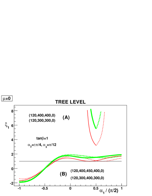
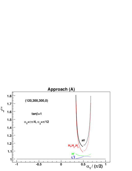
Figure 1: The trilinear coupling ratio ξ1subscript𝜉1\xi_{1} defined in (30) at the tree level plotted as a function of α1subscript𝛼1\alpha_{1} for both the approaches (A) and (B), for two different values of α2subscript𝛼2\alpha_{2} (π/4𝜋4-\pi/4, dashed, and +π/4𝜋4+\pi/4, solid), both with α3=π/12subscript𝛼3𝜋12\alpha_{3}=\pi/12. The masses of the Higgs bosons are M1=120GeVsubscript𝑀1120GeVM_{1}=120~{}\text{GeV}, with M2=MH±=300GeVsubscript𝑀2subscript𝑀superscript𝐻plus-or-minus300GeVM_{2}=M_{H^{\pm}}=300~{}\text{GeV} (red, thin lines), and M2=MH±=400GeVsubscript𝑀2subscript𝑀superscript𝐻plus-or-minus400GeVM_{2}=M_{H^{\pm}}=400~{}\text{GeV} (green, heavy lines). Furthermore, μ=0𝜇0\mu=0 and tanβ=1𝛽1\tan\beta=1. The numbers in insets give values of (M1,M2,MH±,μ)subscript𝑀1subscript𝑀2subscript𝑀superscript𝐻plus-or-minus𝜇(M_{1},M_{2},M_{H^{\pm}},\mu) for approach (A) and for those of (M1,M2,M3,MH±,μ)subscript𝑀1subscript𝑀2subscript𝑀3subscript𝑀superscript𝐻plus-or-minus𝜇(M_{1},M_{2},M_{3},M_{H^{\pm}},\mu) for approach (B).

Within an allowed domain in the parameter space, the trilinear couplings can have a very strong dependence on the neutral Higgs boson mixing angles, as is illustrated in Fig. 1, where we have plotted ξ1subscript𝜉1\xi_{1} as a function of α1subscript𝛼1\alpha_{1}, keeping α2=±π/4subscript𝛼2plus-or-minus𝜋4\alpha_{2}=\pm\pi/4 and α3=π/12subscript𝛼3𝜋12\alpha_{3}=\pi/12 fixed.

In this figure, the values of the trilinear coupling are calculated at tree level with M1=120GeVsubscript𝑀1120GeVM_{1}=120~{}\text{GeV}, μ=0𝜇0\mu=0, tanβ=1𝛽1\tan\beta=1, α2=±π/4,subscript𝛼2plus-or-minus𝜋4\alpha_{2}=\pm\pi/4, and α3=π/12subscript𝛼3𝜋12\alpha_{3}=\pi/12. The upper set of lines in this figure (larger values of the trilinear couplings) refer to the approach (A) of Sec. II.2, where we take λ6=λ7=0subscript𝜆6subscript𝜆70\lambda_{6}=\lambda_{7}=0, and fix M2=MH±=300GeVsubscript𝑀2subscript𝑀superscript𝐻plus-or-minus300GeVM_{2}=M_{H^{\pm}}=300~{}\text{GeV}, or M2=MH±=400GeVsubscript𝑀2subscript𝑀superscript𝐻plus-or-minus400GeVM_{2}=M_{H^{\pm}}=400~{}\text{GeV}, as indicated in the caption. The lower set of lines refer to the approach (B), where we fix (M2,M3,MH±)subscript𝑀2subscript𝑀3subscript𝑀superscript𝐻plus-or-minus(M_{2},M_{3},M_{H^{\pm}}) equal to (300,400,300)GeV300400300GeV(300,400,300)~{}\text{GeV}, or (400,450,400)GeV400450400GeV(400,450,400)~{}\text{GeV}, with the additional constraints Imλ5=0Imsubscript𝜆50{\rm Im\thinspace}\lambda_{5}=0, Reλ6=Reλ7=0Resubscript𝜆6Resubscript𝜆70{\rm Re\thinspace}\lambda_{6}={\rm Re\thinspace}\lambda_{7}=0.

From this figure we note a marked qualitative difference between the values of the trilinear coupling calculated via the two approaches of specifying the input parameters. In general, they both lead to solutions for only limited ranges of α1subscript𝛼1\alpha_{1}, keeping M3subscript𝑀3M_{3} fixed [approach (B)], the variation of the coupling with α1subscript𝛼1\alpha_{1} is modest, whereas when λ6=λ7=0subscript𝜆6subscript𝜆70\lambda_{6}=\lambda_{7}=0 and M3subscript𝑀3M_{3} is calculated [approach (A)], the variation with α1subscript𝛼1\alpha_{1} is quite strong (upper part of the figure).

The different behavior of the trilinear coupling in the two approaches can be understood as follows. The trilinear couplings are linear functions of the quartic couplings λisubscript𝜆𝑖\lambda_{i} in the Higgs potential (3). In both the approaches, (A) and (B), the couplings λisubscript𝜆𝑖\lambda_{i} are rather smooth functions of α1subscript𝛼1\alpha_{1}. They are also comparable in magnitude, with the exception that in approach (B), where we fix M3subscript𝑀3M_{3}, we also take as input Imλ5=0Imsubscript𝜆50{\rm Im\thinspace}\lambda_{5}=0. Thus, the role played by Imλ5Imsubscript𝜆5{\rm Im\thinspace}\lambda_{5} in approach (A) is played by Imλ6Imsubscript𝜆6{\rm Im\thinspace}\lambda_{6} and Imλ7Imsubscript𝜆7{\rm Im\thinspace}\lambda_{7} in approach (B). This switch of role from Imλ5Imsubscript𝜆5{\rm Im\thinspace}\lambda_{5} to Imλ6Imsubscript𝜆6{\rm Im\thinspace}\lambda_{6} and Imλ7Imsubscript𝜆7{\rm Im\thinspace}\lambda_{7} has as a consequence, for the case studied in Fig. 1, that a333subscript𝑎333a_{333} (which is quite large) switches sign. Since the coefficient in (III.1) that relates a333subscript𝑎333a_{333} to λ111subscript𝜆111\lambda_{111} is essentially R133superscriptsubscript𝑅133R_{13}^{3}, with R13=sinα2=±1/2subscript𝑅13subscript𝛼2plus-or-minus12R_{13}=\sin\alpha_{2}=\pm 1/\sqrt{2}, this sign change of the large coupling a333subscript𝑎333a_{333} is the dominant effect which causes the difference between the parameter choices in the approaches (A) and (B) (for the set of parameters considered). In fact, truncating Eq. (III.1) with a333=0subscript𝑎3330a_{333}=0, one finds the ratio of the couplings ξ1=3.85subscript𝜉13.85\xi_{1}=3.8-5 for approach (A), and 3.63.83.63.83.6-3.8 for approach (B), where we have taken M1=120GeVsubscript𝑀1120GeVM_{1}=120~{}\text{GeV}, M2=400GeVsubscript𝑀2400GeVM_{2}=400~{}\text{GeV}, α2=π/4subscript𝛼2𝜋4\alpha_{2}=-\pi/4, and α4=π/12subscript𝛼4𝜋12\alpha_{4}=\pi/12 for both the approaches. Thus, one may conclude that the two different ways of introducing CP violation in the two Higgs doublet model lead to very different values for the trilinear coupling λ111subscript𝜆111\lambda_{111}.

Furthermore, we note that Reλ5Resubscript𝜆5{\rm Re\thinspace}\lambda_{5} depends on α1subscript𝛼1\alpha_{1} through M3subscript𝑀3M_{3} only ElKaffas:2007rq . Thus, in approach (A), with M3subscript𝑀3M_{3} depending on α1subscript𝛼1\alpha_{1}, the resulting Reλ5Resubscript𝜆5{\rm Re\thinspace}\lambda_{5} will also vary, whereas in approach (B), Reλ5Resubscript𝜆5{\rm Re\thinspace}\lambda_{5} is constant. This contributes to the stronger variation of ξ1subscript𝜉1\xi_{1} with α1subscript𝛼1\alpha_{1} in approach (A).

In view of the strong dependence of the trilinear couplings on the mixing angles, we shall henceforth average over these angles within the allowed ranges. In Figs. 2 and 3 we show the tree-level ratios

ξ1=λ111λHHHSM,ξ2=λ112λHHHSM,formulae-sequencedelimited-⟨⟩subscript𝜉1delimited-⟨⟩subscript𝜆111subscriptsuperscript𝜆SM𝐻𝐻𝐻delimited-⟨⟩subscript𝜉2delimited-⟨⟩subscript𝜆112subscriptsuperscript𝜆SM𝐻𝐻𝐻\langle\xi_{1}\rangle=\frac{\langle\lambda_{111}\rangle}{\lambda^{\text{SM}}_{HHH}},\quad\langle\xi_{2}\rangle=\frac{\langle\lambda_{112}\rangle}{\lambda^{\text{SM}}_{HHH}}, (43)

for a representative choice of parameter sets. These are averages, obtained by scanning over the 𝜶=(α1,α2,α3)𝜶subscript𝛼1subscript𝛼2subscript𝛼3{\boldsymbol{\alpha}}=(\alpha_{1},\alpha_{2},\alpha_{3}) space, subjecting all model points to positivity, unitarity, and the experimental constraints discussed above, working within the approach (A) defined in Sec. II.2, and normalizing them with respect to the SM coupling, as defined in Eq. (30). The scans are performed over 200×200×100200200100200\times 200\times 100 points.

Before considering the general case of arbitrary CP violation, we first consider, in Fig. 2, a region of parameter space near the limit (18) of no CP violation:

|α2|α0,|α3|α0,α0=0.05×π/2,formulae-sequencesubscript𝛼2subscript𝛼0formulae-sequencesubscript𝛼3subscript𝛼0subscript𝛼00.05𝜋2|\alpha_{2}|\leq\alpha_{0},\quad|\alpha_{3}|\leq\alpha_{0},\quad\alpha_{0}=0.05\times\pi/2, (44)

referred to as “minimal CP violation”. From the above discussion (see Eqs. (III.1.1)–(35)), it follows that this corresponds to a domain of parameters close to the CP-conserving Higgs sector of the MSSM. We note that the approach (A), where we determine M3subscript𝑀3M_{3} from M1subscript𝑀1M_{1}, M2subscript𝑀2M_{2} and the rotation matrix, does not permit us to go all the way to the limit α2=α3=0subscript𝛼2subscript𝛼30\alpha_{2}=\alpha_{3}=0.

Refer to caption
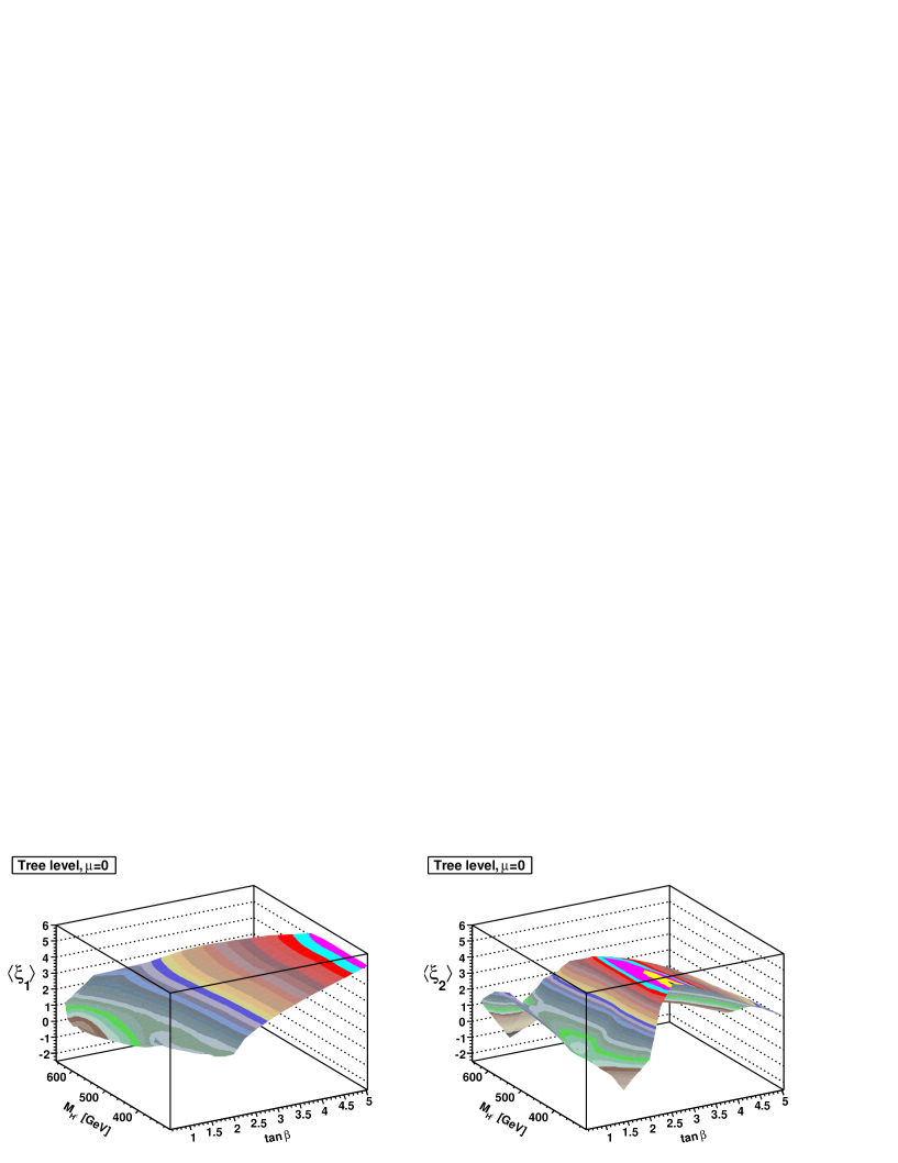
Figure 2: Trilinear Higgs coupling ratios ξ1delimited-⟨⟩subscript𝜉1\langle\xi_{1}\rangle and ξ2delimited-⟨⟩subscript𝜉2\langle\xi_{2}\rangle as defined in Eq. (43) at the tree-level, in approach (A), for the values of the Higgs masses M1=120GeVsubscript𝑀1120GeVM_{1}=120~{}\text{GeV}, M2=300GeVsubscript𝑀2300GeVM_{2}=300~{}\text{GeV} and μ=0𝜇0\mu=0. The ratios are plotted for the case of the CP-conserving MSSM-like limit as defined in Eq. (44).
Refer to caption
Refer to caption
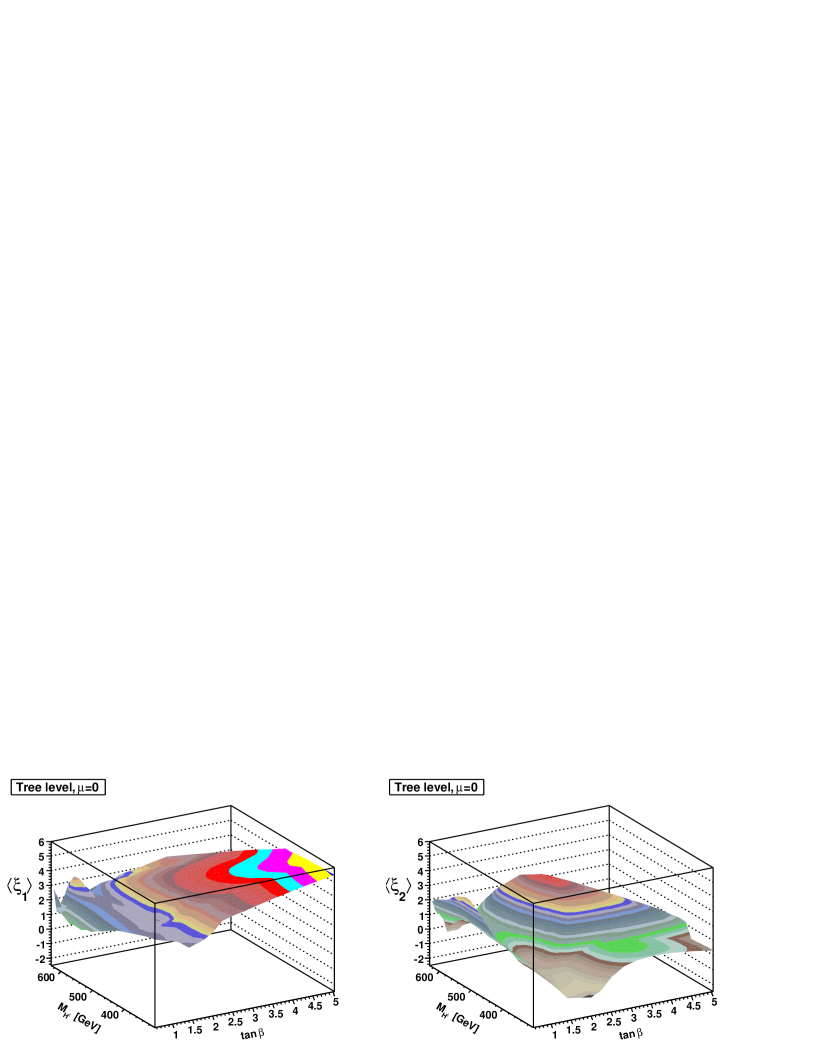
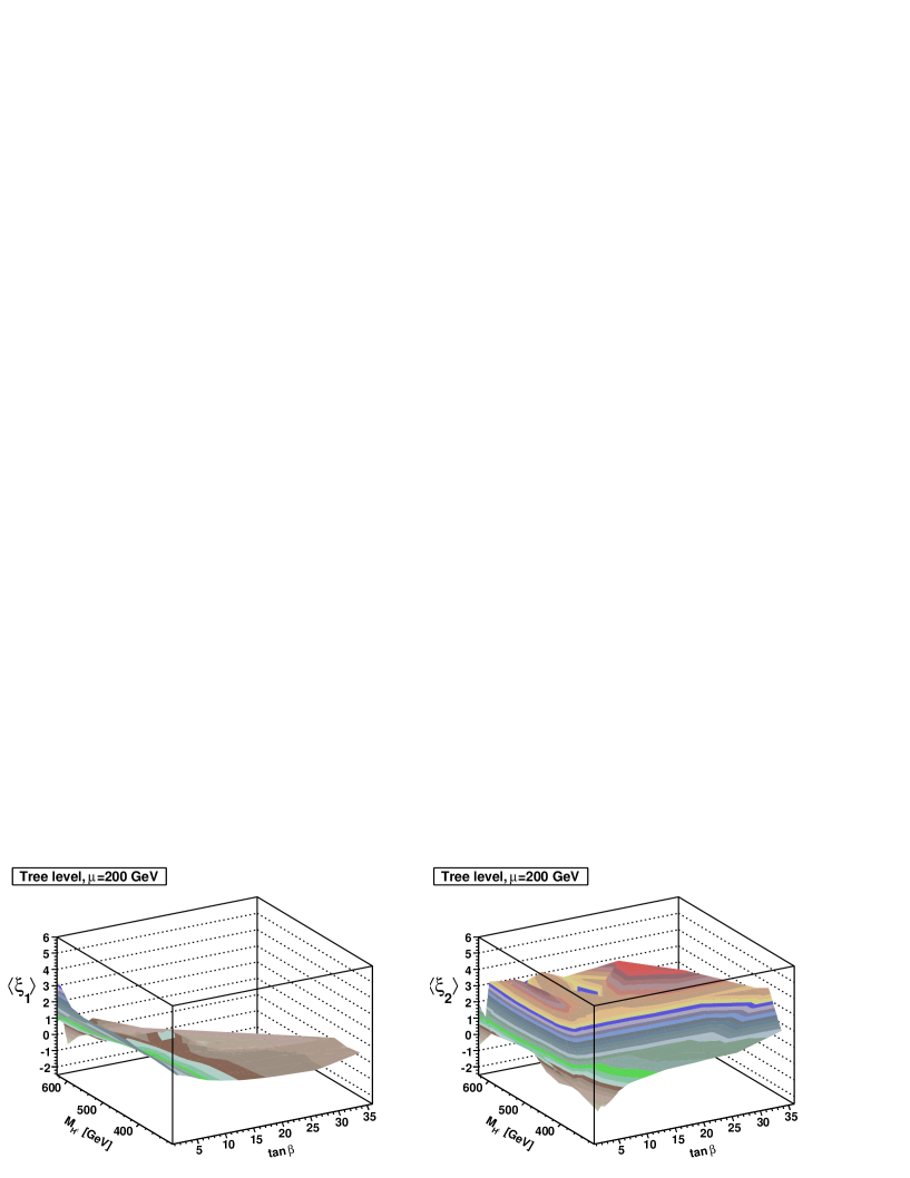
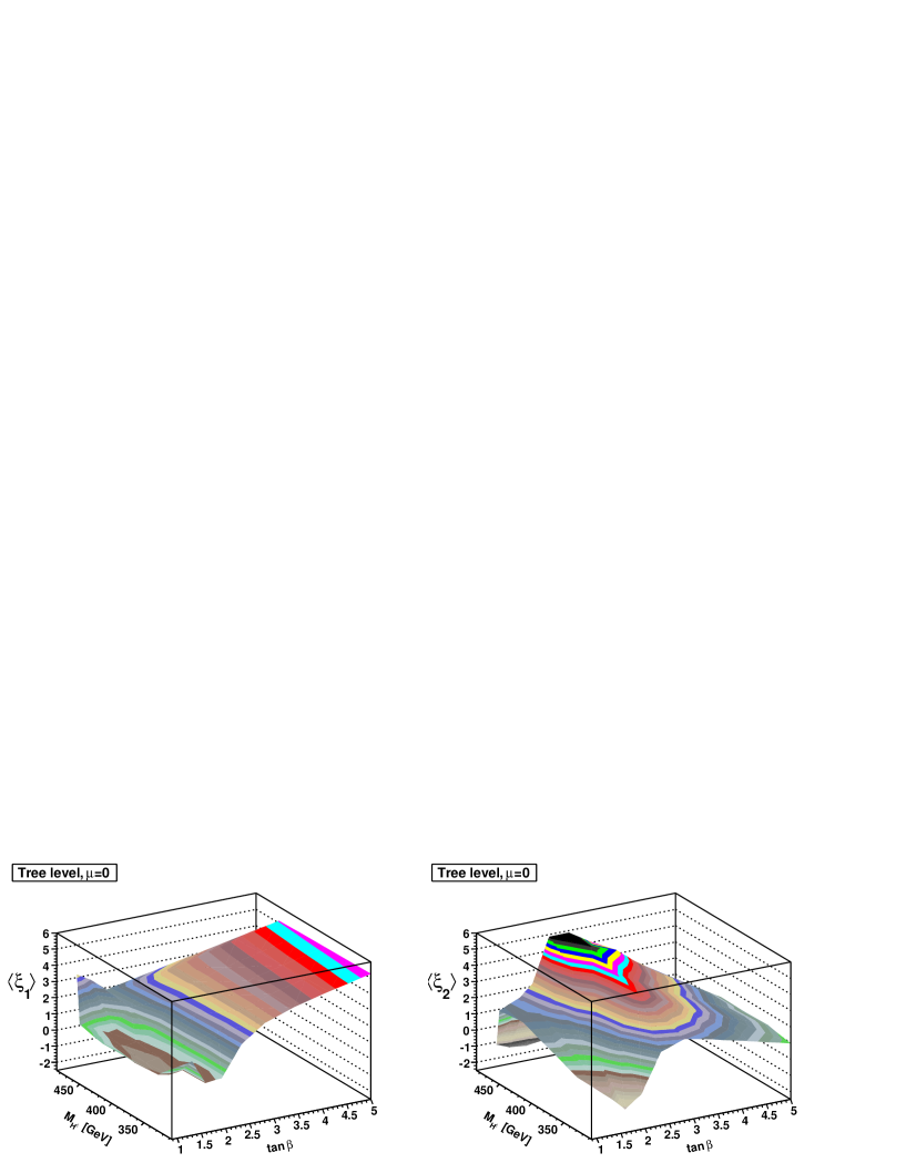
Figure 3: Tree-level trilinear coupling ratios ξ1delimited-⟨⟩subscript𝜉1\langle\xi_{1}\rangle and ξ2delimited-⟨⟩subscript𝜉2\langle\xi_{2}\rangle as defined in Eq. (43), in approach (A), for the values of the Higgs masses M1=120GeVsubscript𝑀1120GeVM_{1}=120~{}\text{GeV} and M2=300GeVsubscript𝑀2300GeVM_{2}=300~{}\text{GeV}. For the top panel μ=0𝜇0\mu=0, whereas for the bottom panel μ=200GeV𝜇200GeV\mu=200~{}\text{GeV}. This plot is for the general case including CP violation, and is compatible with general constraints on the model.

In this figure, which is valid for μ=0𝜇0\mu=0, the plots do not extend much beyond tanβ=5𝛽5\tan\beta=5. This is caused by the constraint of unitarity in the Higgs–Higgs scattering sector WahabElKaffas:2007xd . At the higher values of tanβ𝛽\tan\beta, there is also a narrowing of the allowed region, largely due to the constraints following from ΔρΔ𝜌\Delta\rho and the B𝐵B physics ElKaffas:2006nt ; WahabElKaffas:2007xd .

The surfaces representing ξ1delimited-⟨⟩subscript𝜉1\langle\xi_{1}\rangle and ξ2delimited-⟨⟩subscript𝜉2\langle\xi_{2}\rangle in Fig. 2 are in fact quite remininscent of the corresponding averages of λ1subscript𝜆1\lambda_{1} and Reλ345Resubscript𝜆345{\rm Re\thinspace}\lambda_{345}, respectively. The details of these correspondences depend on which domains of the 𝜶𝜶{\boldsymbol{\alpha}} space (in this case, α1subscript𝛼1\alpha_{1}) is populated. Typically, only scattered regions are allowed ElKaffas:2006nt .

On the other hand, in Fig. 3 we have scanned over the full range of values of α2subscript𝛼2\alpha_{2} and α3subscript𝛼3\alpha_{3}, compatible with all the constraints.

From these figures, we see that in much of the tanβMH±𝛽subscript𝑀superscript𝐻plus-or-minus\tan\beta-M_{H^{\pm}} parameter space, there is a considerable enhancement of the trilinear couplings as compared with the corresponding trilinear coupling in the SM. This is consistent with the special case studied in Fig. 1.

Incorporating CP violation in the 2HDM, we see a considerable change in the behavior of the couplings as we go from Fig. 2 to Fig. 3. This reflects the fact seen in Fig. 1 that the couplings have a strong dependence on the mixing angles, and, thus, on how CP violation is incorporated in the model.

Furthermore, there is a rapid variation of the Higgs coupling ratios around tanβ=𝒪(2)𝛽𝒪2\tan\beta={\cal O}(2). As we shall see in the following, this is accompanied by a strong variation as one scans across the different values of 𝜶𝜶{\boldsymbol{\alpha}}.

Refer to caption
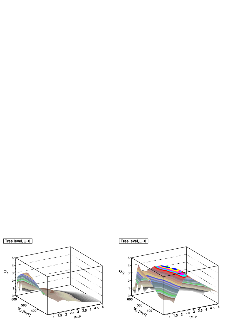
Figure 4: Variance of trilinear coupling ratios ξ1subscript𝜉1\xi_{1} and ξ2subscript𝜉2\xi_{2} at the tree level. The parameters here correspond to the upper panels (μ=0𝜇0\mu=0) of Fig. 3.
Refer to caption
Figure 5: Trilinear coupling ratios ξ1delimited-⟨⟩subscript𝜉1\langle\xi_{1}\rangle and ξ2delimited-⟨⟩subscript𝜉2\langle\xi_{2}\rangle at the tree level [see Eq. (43)], for approach (B), with M1=120GeVsubscript𝑀1120GeVM_{1}=120~{}\text{GeV}, M2=300GeVsubscript𝑀2300GeVM_{2}=300~{}\text{GeV}, M3=400GeVsubscript𝑀3400GeVM_{3}=400~{}\text{GeV} and μ=0𝜇0\mu=0.

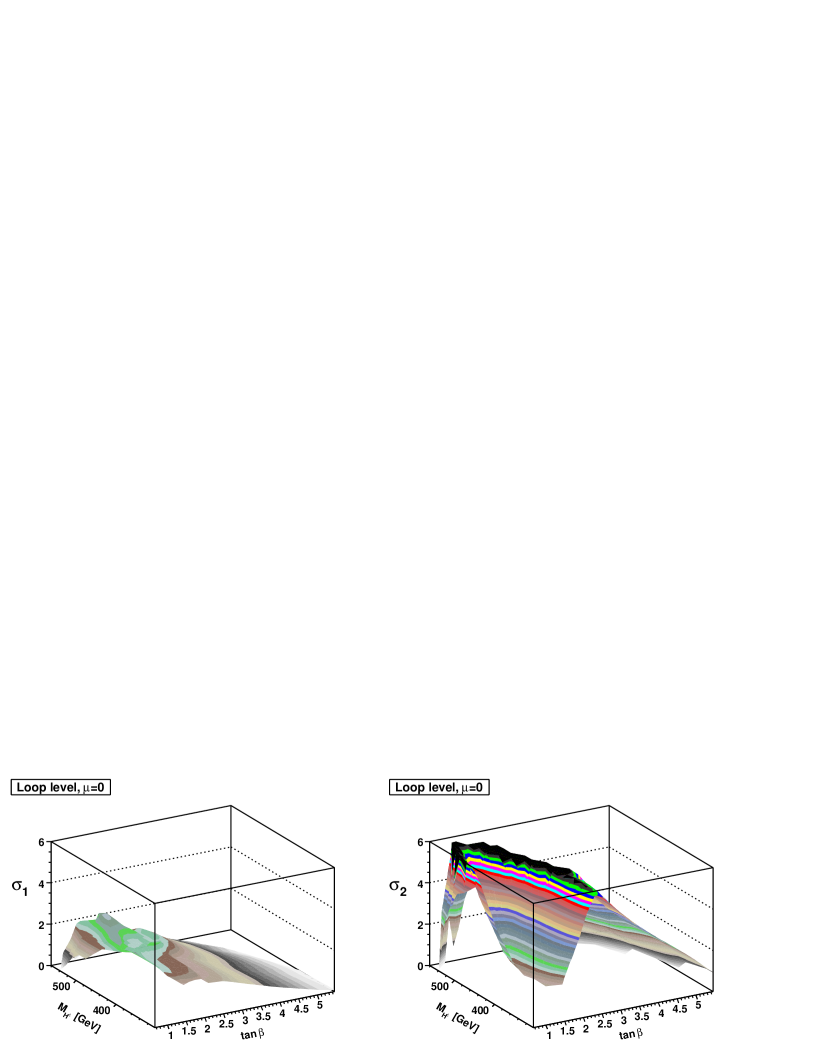
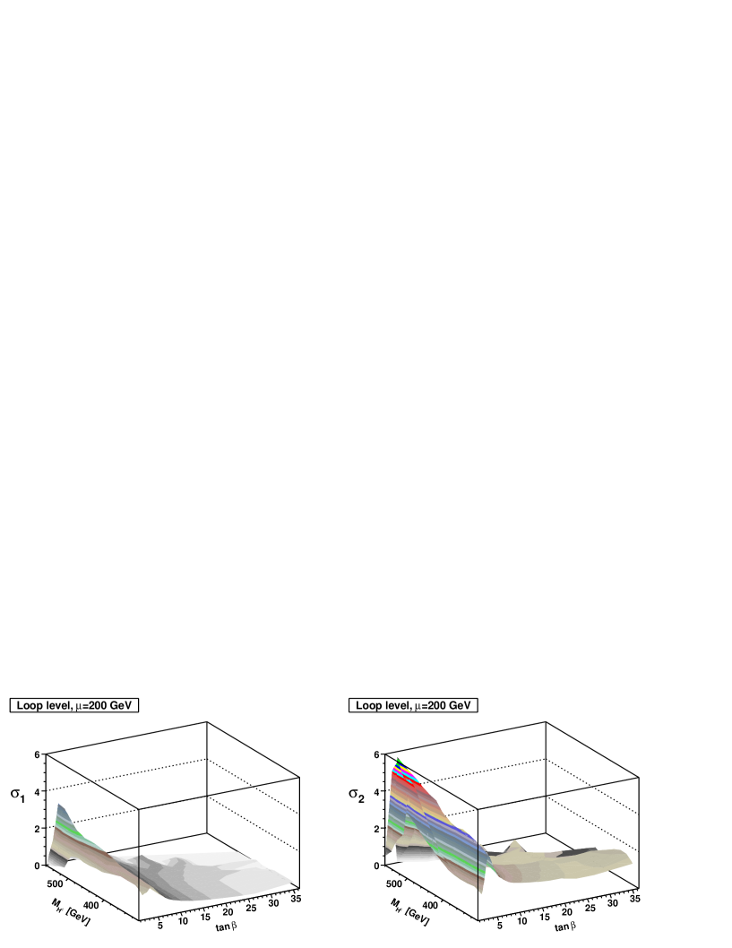
The trilinear coupling has a rather complicated behaviour across the tanβ𝛽\tan\betaMH±subscript𝑀superscript𝐻plus-or-minusM_{H^{\pm}} plane, despite the smoothening that is implicit in the averaging over 𝜶𝜶{\boldsymbol{\alpha}}. As is evident from Fig. 1 for ξ1subscript𝜉1\xi_{1}, the ratios ξ1subscript𝜉1\xi_{1} and ξ2subscript𝜉2\xi_{2} of trilinear couplings also vary considerably over the parameter space of 𝜶𝜶{\boldsymbol{\alpha}}. One measure of this variation is the variance, defined as

σi=(ξiξi)2.subscript𝜎𝑖delimited-⟨⟩superscriptsubscript𝜉𝑖delimited-⟨⟩subscript𝜉𝑖2\sigma_{i}=\sqrt{\langle(\xi_{i}-\langle\xi_{i}\rangle)^{2}\rangle}. (45)

In Fig. 4 we display the variances σ1subscript𝜎1\sigma_{1} and σ2subscript𝜎2\sigma_{2} corresponding to the upper panels of Fig. 3. This quantity (in units of the SM trilinear coupling) is seen to be quite considerable, in particular for ξ2subscript𝜉2\xi_{2} and for moderate values of tanβ𝛽\tan\beta.

For approach (B), when we keep all three neutral Higgs boson masses fixed, the behaviour is smoother, as seen in Fig. 5. For the parameters considered (note that μ=0𝜇0\mu=0), the values of tanβ𝛽\tan\beta extend up to about 5. We note that the quantity ξ1delimited-⟨⟩subscript𝜉1\langle\xi_{1}\rangle is rather similar to that shown in Figs. 2 and 3, increasing more or less monotonically with tanβ𝛽\tan\beta. The ratio ξ2delimited-⟨⟩subscript𝜉2\langle\xi_{2}\rangle differs more, exhibiting a bulge of rather strong H1H1H2subscript𝐻1subscript𝐻1subscript𝐻2H_{1}H_{1}H_{2} coupling for tanβ=23𝛽23\tan\beta=2-3 and MH±=450500GeVsubscript𝑀superscript𝐻plus-or-minus450500GeVM_{H^{\pm}}=450-500~{}\text{GeV}.

III.2 Charged–Charged–Neutral Higgs Couplings

Although in this paper we are mainly concerned with the trilinear couplings of the neutral Higgs bosons, here we briefly discuss the trilinear couplings of the charged Higgs boson of the 2HDM Carena:2002bb . These are given by

λi+=m=1,2,3Rimbm.subscript𝜆limit-from𝑖subscript𝑚123subscript𝑅𝑖𝑚subscript𝑏𝑚\lambda_{i+-}=\sum_{m=1,2,3}R_{im}\,b_{m}. (46)

We note that the index m𝑚m (like the indices n𝑛n and o𝑜o in Eq. (III.1)) refers to the weak interaction eigenstates (η1subscript𝜂1\eta_{1}, η2subscript𝜂2\eta_{2} and η3subscript𝜂3\eta_{3}) of Eq. (5). The coefficients bmsubscript𝑏𝑚b_{m} in (46) can be written as (in units of iv𝑖𝑣-iv):

b1subscript𝑏1\displaystyle b_{1} =cosβ{sin2β(λ1λ4Reλ5)+cos2βλ3\displaystyle=\cos\beta\{\sin^{2}\beta\,(\lambda_{1}-\lambda_{4}-{\rm Re\thinspace}\lambda_{5})+\cos^{2}\beta\,\lambda_{3}
+cosβsinβ[(tan2β2)Reλ6+Reλ7]},\displaystyle+\cos\beta\,\sin\beta\,[(\tan^{2}\beta-2)\,{\rm Re\thinspace}\lambda_{6}+{\rm Re\thinspace}\lambda_{7}]\},
b2subscript𝑏2\displaystyle b_{2} =sinβ{cos2β(λ2λ4Reλ5)+sin2βλ3\displaystyle=\sin\beta\{\cos^{2}\beta\,(\lambda_{2}-\lambda_{4}-{\rm Re\thinspace}\lambda_{5})+\sin^{2}\beta\,\lambda_{3}
+cosβsinβ[Reλ6+(cot2β2)Reλ7]},\displaystyle+\cos\beta\,\sin\beta\,[{\rm Re\thinspace}\lambda_{6}+(\cot^{2}\beta-2)\,{\rm Re\thinspace}\lambda_{7}]\},
b3subscript𝑏3\displaystyle b_{3} =cosβsinβImλ5sin2βImλ6cos2βImλ7.absent𝛽𝛽Imsubscript𝜆5superscript2𝛽Imsubscript𝜆6superscript2𝛽Imsubscript𝜆7\displaystyle=\cos\beta\,\sin\beta\,{\rm Im\thinspace}\lambda_{5}-\sin^{2}\beta\,{\rm Im\thinspace}\lambda_{6}-\cos^{2}\beta\,{\rm Im\thinspace}\lambda_{7}. (47)

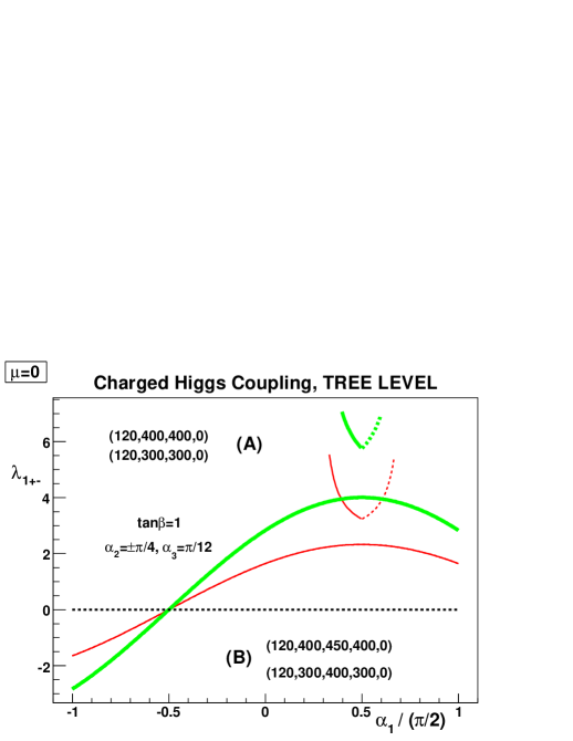
In Fig. 6 we display the coupling of H1subscript𝐻1H_{1} to the charged H+Hsuperscript𝐻superscript𝐻H^{+}H^{-} pair, for the same choice of parameters as in Fig. 1. We note that in approach (B), with tanβ=1𝛽1\tan\beta=1 and Imλ5=0Imsubscript𝜆50{\rm Im\thinspace}\lambda_{5}=0, this coupling has two interesting features: (1) It does not depend on the sign of α2subscript𝛼2\alpha_{2}; and (2) it passes through zero for α1=π/4subscript𝛼1𝜋4\alpha_{1}=-\pi/4. The independence from the sign of α2subscript𝛼2\alpha_{2} can be understood in the following manner. For i=1𝑖1i=1, the first two terms in Eq. (46) (proportional to R11subscript𝑅11R_{11} and R12subscript𝑅12R_{12}) contribute terms which are odd in α2subscript𝛼2\alpha_{2}, arising from λ1subscript𝜆1\lambda_{1}, λ2subscript𝜆2\lambda_{2} and λ3subscript𝜆3\lambda_{3}. These odd parts are proportional to (M32M22)superscriptsubscript𝑀32superscriptsubscript𝑀22(M_{3}^{2}-M_{2}^{2}), and cancel against odd parts coming from the third term in (46), which are proportional to Imλ6+Imλ7Imsubscript𝜆6Imsubscript𝜆7{\rm Im\thinspace}\lambda_{6}+{\rm Im\thinspace}\lambda_{7}, which in turn is proportional to 13+23subscript13subscript23{\cal M}_{13}+{\cal M}_{23}.

Furthermore, the vanishing of the coupling at α1=π/4subscript𝛼1𝜋4\alpha_{1}=-\pi/4 can be understood as follows. In approach (B), with tanβ=1𝛽1\tan\beta=1 and α1=π/4subscript𝛼1𝜋4\alpha_{1}=-\pi/4, we have (see Eqs. (3.1) and (3.2) of Ref. ElKaffas:2007rq )

λ1(α2,α3)subscript𝜆1subscript𝛼2subscript𝛼3\displaystyle\lambda_{1}(\alpha_{2},\alpha_{3}) =1v2[c22M12+(c3s2s3)2M22\displaystyle=\frac{1}{v^{2}}[c_{2}^{2}M_{1}^{2}+(c_{3}-s_{2}s_{3})^{2}M_{2}^{2}
+(s3+s2c3)2M32μ2],\displaystyle+(s_{3}+s_{2}c_{3})^{2}M_{3}^{2}-\mu^{2}],
λ2(α2,α3)subscript𝜆2subscript𝛼2subscript𝛼3\displaystyle\lambda_{2}(\alpha_{2},\alpha_{3}) =1v2[c22M12+(c3+s2s3)2M22\displaystyle=\frac{1}{v^{2}}[c_{2}^{2}M_{1}^{2}+(c_{3}+s_{2}s_{3})^{2}M_{2}^{2}
+(s3s2c3)2M32μ2].\displaystyle+(s_{3}-s_{2}c_{3})^{2}M_{3}^{2}-\mu^{2}]. (48)

Thus, for these particular values of tanβ𝛽\tan\beta and α1subscript𝛼1\alpha_{1}, λ2(α2,α3)=λ1(α2,α3)subscript𝜆2subscript𝛼2subscript𝛼3subscript𝜆1subscript𝛼2subscript𝛼3\lambda_{2}(-\alpha_{2},\alpha_{3})=\lambda_{1}(\alpha_{2},\alpha_{3}), the first two terms in Eq. (46) cancel, and we are left with

λ1+=R13b3=12s2(Imλ5Imλ6Imλ7)=0,subscript𝜆limit-from1subscript𝑅13subscript𝑏312subscript𝑠2Imsubscript𝜆5Imsubscript𝜆6Imsubscript𝜆70\lambda_{1+-}=R_{13}b_{3}={\textstyle\frac{1}{2}}s_{2}({\rm Im\thinspace}\lambda_{5}-{\rm Im\thinspace}\lambda_{6}-{\rm Im\thinspace}\lambda_{7})=0, (49)

where in the last step we have used Imλ5=0Imsubscript𝜆50{\rm Im\thinspace}\lambda_{5}=0, and the relations (see Eq. (II.2))

Imλ5+Imλ6+Imλ7=2v2[132+232],Imsubscript𝜆5Imsubscript𝜆6Imsubscript𝜆72superscript𝑣2delimited-[]superscriptsubscript132superscriptsubscript232{\rm Im\thinspace}\lambda_{5}+{\rm Im\thinspace}\lambda_{6}+{\rm Im\thinspace}\lambda_{7}=-\frac{\sqrt{2}}{v^{2}}[{\cal M}_{13}^{2}+{\cal M}_{23}^{2}], (50)

valid for tanβ=1𝛽1\tan\beta=1, and

132+232=0,superscriptsubscript132superscriptsubscript2320{\cal M}_{13}^{2}+{\cal M}_{23}^{2}=0, (51)

valid for α1=π/4subscript𝛼1𝜋4\alpha_{1}=-\pi/4.

Refer to caption
Figure 6: The trilinear coupling λ1+subscript𝜆limit-from1\lambda_{1+-} at the tree level as a function of α1subscript𝛼1\alpha_{1}, for two different values of α2subscript𝛼2\alpha_{2} (π/4𝜋4-\pi/4, dashed, and +π/4𝜋4+\pi/4, solid), both with α3=π/12subscript𝛼3𝜋12\alpha_{3}=\pi/12. The masses and parameters are the same as in Fig. 1.

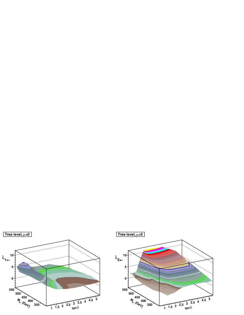
In Fig. 7, we show the coupling of the lightest neutral Higgs bosons to the charged Higgs bosons, averaged over 𝜶𝜶{\boldsymbol{\alpha}}, in approach (A). Corresponding to what we observed in Fig. 6, these averages over 𝜶𝜶{\boldsymbol{\alpha}} also vanish along certain lines in the parameter space.
Refer to caption
Figure 7: Tree-level trilinear couplings λ1+subscript𝜆limit-from1\lambda_{1+-} and λ2+subscript𝜆limit-from2\lambda_{2+-} (in units of iv𝑖𝑣-iv) of the two lightest neutral Higgs bosons, H1subscript𝐻1H_{1} and H2subscript𝐻2H_{2}, to a charged pair for M1=120GeVsubscript𝑀1120GeVM_{1}=120~{}\text{GeV}, M2=300GeVsubscript𝑀2300GeVM_{2}=300~{}\text{GeV} and μ=0𝜇0\mu=0. The couplings are averaged over 𝜶𝜶{\boldsymbol{\alpha}}, and have been plotted for approach (A).

IV One-loop Corrections to the Higgs Boson Masses

IV.1 One-loop effective potential

For a realistic computation of the Higgs boson properties in the 2HDM, we must take into account the one-loop radiative corrections to the tree-level potential (3). When this is done, the relations among masses and the couplings of the tree-level potential undergo a change. In the MSSM, this effect, which is dominated by the top (and stop) quark contributions, is known to be very important Okada:1990vk (see also Ref. Ham:2002ps ). In the 2HDM, there being no one-loop contribution from squarks, the main contributions at one loop are generated by the Higgs bosons. We shall here study the one-loop radiative corrections to the neutral Higgs sector using the method of one-loop effective potential Coleman:1973jx . The one-loop corrections to the tree-level potential (3) are given by

ΔVΔ𝑉\displaystyle\Delta V =164π2[bosonsM4(logM2Q232)\displaystyle=\frac{1}{64\pi^{2}}\biggl{[}\sum_{\text{bosons}}M^{4}\biggl{(}\log\frac{M^{2}}{Q^{2}}-\frac{3}{2}\biggr{)}
fermionsM4(logM2Q232)],\displaystyle-\sum_{\text{fermions}}M^{4}\biggl{(}\log\frac{M^{2}}{Q^{2}}-\frac{3}{2}\biggr{)}\biggr{]}, (52)

where the sums run over all bosonic and fermionic degrees of freedom, respectively, and Q2superscript𝑄2Q^{2} represents the scale at which the couplings are evaluated. As indicated above, the dominant contributions to (IV.1) come from the Higgs bosons (neutral and charged), and the top quarks, all of which we will calculate in this section. Taking into account the spin, charge and color degrees of freedom, we obtain

ΔVΔ𝑉\displaystyle\Delta V =ΔVneutral Higgs+ΔVcharged Higgs+ΔVtopabsentΔsubscript𝑉neutral HiggsΔsubscript𝑉charged HiggsΔsubscript𝑉top\displaystyle=\Delta V_{\text{neutral Higgs}}+\Delta V_{\text{charged Higgs}}+\Delta V_{\text{top}}
=164π2=13[M4(logM2Q232)]absent164superscript𝜋2superscriptsubscript13delimited-[]superscriptsubscript𝑀4superscriptsubscript𝑀2superscript𝑄232\displaystyle=\frac{1}{64\pi^{2}}\sum_{\ell=1}^{3}\biggl{[}M_{\ell}^{4}\biggl{(}\log\frac{M_{\ell}^{2}}{Q^{2}}-\frac{3}{2}\biggr{)}\biggr{]}
+132π2MH±4(logMH±2Q232)132superscript𝜋2superscriptsubscript𝑀superscript𝐻plus-or-minus4superscriptsubscript𝑀superscript𝐻plus-or-minus2superscript𝑄232\displaystyle+\frac{1}{32\pi^{2}}M_{H^{\pm}}^{4}\biggl{(}\log\frac{M_{H^{\pm}}^{2}}{Q^{2}}-\frac{3}{2}\biggr{)}
316π2mt4(logmt2Q232),316superscript𝜋2superscriptsubscript𝑚𝑡4superscriptsubscript𝑚𝑡2superscript𝑄232\displaystyle-\frac{3}{16\pi^{2}}\,m_{t}^{4}\biggl{(}\log\frac{m_{t}^{2}}{Q^{2}}-\frac{3}{2}\biggr{)}, (53)

where all masses are understood to be field-dependent masses. Thus, after differentiation analogous to the one in Eq. (10) for the tree-level potential, for example, we do not set the fields η1subscript𝜂1\eta_{1}, η2subscript𝜂2\eta_{2} and η3subscript𝜂3\eta_{3} to zero, but instead evaluate

ij2(η1,η2,η3)=ηiηjV(η1,η2,η3,H±,G±),subscriptsuperscript2𝑖𝑗subscript𝜂1subscript𝜂2subscript𝜂3subscript𝜂𝑖subscript𝜂𝑗𝑉subscript𝜂1subscript𝜂2subscript𝜂3superscript𝐻plus-or-minussuperscript𝐺plus-or-minus{\cal M}^{2}_{ij}(\eta_{1},\eta_{2},\eta_{3})=\frac{\partial}{\partial\eta_{i}}\frac{\partial}{\partial\eta_{j}}\,V(\eta_{1},\eta_{2},\eta_{3},H^{\pm},G^{\pm}), (54)

and similarly

MH±2(η1,η2,η3)=H+HV(η1,η2,η3,H±,G±),superscriptsubscript𝑀superscript𝐻plus-or-minus2subscript𝜂1subscript𝜂2subscript𝜂3superscript𝐻superscript𝐻𝑉subscript𝜂1subscript𝜂2subscript𝜂3superscript𝐻plus-or-minussuperscript𝐺plus-or-minusM_{H^{\pm}}^{2}(\eta_{1},\eta_{2},\eta_{3})=\frac{\partial}{\partial H^{+}}\frac{\partial}{\partial H^{-}}\,V(\eta_{1},\eta_{2},\eta_{3},H^{\pm},G^{\pm}), (55)

and after having performed the differentiation, we set H±=G±=0.superscript𝐻plus-or-minussuperscript𝐺plus-or-minus0H^{\pm}=G^{\pm}=0.

At tree level, the three minimization conditions (19) (two real, and one imaginary) can be used to eliminate the bilinear parameters m12superscriptsubscript𝑚12m_{1}^{2} and m22superscriptsubscript𝑚22m_{2}^{2}, as well as relate Imλ5Imsubscript𝜆5{\rm Im\thinspace}\lambda_{5} to Imm122Imsuperscriptsubscript𝑚122{\rm Im\thinspace}m_{12}^{2}. At the one-loop level, the expressions for m12superscriptsubscript𝑚12m_{1}^{2} and m22superscriptsubscript𝑚22m_{2}^{2} are modified due to the contributions coming from ΔV/η1Δ𝑉subscript𝜂1\partial\Delta V/\partial\eta_{1} and ΔV/η2Δ𝑉subscript𝜂2\partial\Delta V/\partial\eta_{2}. This amounts to adjusting the parameters of the potential such that the minimum is stationary in terms of the same vacuum expectation values v1subscript𝑣1v_{1} and v2subscript𝑣2v_{2} as for the tree-level potential (i.e., tanβ𝛽\tan\beta remains unchanged). In the following we shall calculate the different contributions to the neutral Higgs boson masses arising from (IV.1) using the above procedure.

IV.2 One-loop corrections to Higgs masses

The mass squared matrix for the neutral Higgs bosons will receive contributions from one-loop effects due to neutral Higgs bosons, which can be written as

2ΔVneutral Higgsηiηjsuperscript2Δsubscript𝑉neutral Higgssubscript𝜂𝑖subscript𝜂𝑗\displaystyle\frac{\partial^{2}\Delta V_{\text{neutral Higgs}}}{\partial\eta_{i}\partial\eta_{j}} =132π2=13[logM2Q2M2ηiM2ηj\displaystyle=\frac{1}{32\pi^{2}}\sum_{\ell=1}^{3}\biggl{[}\log\frac{M_{\ell}^{2}}{Q^{2}}\frac{\partial M_{\ell}^{2}}{\partial\eta_{i}}\frac{\partial M_{\ell}^{2}}{\partial\eta_{j}}
+M2(logM2Q21)2M2ηiηj].\displaystyle+M_{\ell}^{2}\biggl{(}\log\frac{M_{\ell}^{2}}{Q^{2}}-1\biggr{)}\frac{\partial^{2}M_{\ell}^{2}}{\partial\eta_{i}\partial\eta_{j}}\biggr{]}. (56)

The derivatives of M2superscriptsubscript𝑀2M_{\ell}^{2} with respect to the fields ηisubscript𝜂𝑖\eta_{i}, which are rather involved, are discussed in detail in Appendix C.

The corresponding second derivatives of the charged-Higgs-field-dependent part of the one-loop corrections to the potential, ΔVcharged HiggsΔsubscript𝑉charged Higgs\Delta V_{\text{charged Higgs}}, in (IV.1) are given by

2ΔVcharged Higgsηiηjsuperscript2Δsubscript𝑉charged Higgssubscript𝜂𝑖subscript𝜂𝑗\displaystyle\frac{\partial^{2}\Delta V_{\text{charged Higgs}}}{\partial\eta_{i}\partial\eta_{j}} =116π2[logMH±2Q2MH±2ηiMH±2ηj\displaystyle=\frac{1}{16\pi^{2}}\biggl{[}\log\frac{M_{H^{\pm}}^{2}}{Q^{2}}\frac{\partial M_{H^{\pm}}^{2}}{\partial\eta_{i}}\frac{\partial M_{H^{\pm}}^{2}}{\partial\eta_{j}}
+MH±2(logMH±2Q21)2MH±2ηiηj].\displaystyle+M_{H^{\pm}}^{2}\biggl{(}\log\frac{M_{H^{\pm}}^{2}}{Q^{2}}-1\biggr{)}\frac{\partial^{2}M_{H^{\pm}}^{2}}{\partial\eta_{i}\partial\eta_{j}}\biggr{]}. (57)

Finally, there are one-loop corrections due to the top quark, which can be written as

2ΔVtopηiηj=32π2mt4v22(2logmt2Q21)δi2δj2,superscript2Δsubscript𝑉topsubscript𝜂𝑖subscript𝜂𝑗32superscript𝜋2superscriptsubscript𝑚𝑡4superscriptsubscript𝑣222superscriptsubscript𝑚𝑡2superscript𝑄21subscript𝛿𝑖2subscript𝛿𝑗2\frac{\partial^{2}\Delta V_{\text{top}}}{\partial\eta_{i}\partial\eta_{j}}=-\frac{3}{2\pi^{2}}\,\frac{m_{t}^{4}}{v_{2}^{2}}\biggl{(}2\log\frac{m_{t}^{2}}{Q^{2}}-1\biggr{)}\delta_{i2}\delta_{j2}, (58)

where in the last equation we have used mt/ηi=(mt/v2)δi2subscript𝑚𝑡subscript𝜂𝑖subscript𝑚𝑡subscript𝑣2subscript𝛿𝑖2\partial m_{t}/\partial\eta_{i}=(m_{t}/v_{2})\delta_{i2}. We neglect the contributions from lighter fermions.

The full one-loop mass-squared matrix for the neutral Higgs bosons can, thus, be written as a sum of four terms:

ij2(η1,η2,η3)subscriptsuperscript2𝑖𝑗subscript𝜂1subscript𝜂2subscript𝜂3\displaystyle{\cal M}^{2}_{ij}(\eta_{1},\eta_{2},\eta_{3}) =tree,ij2(η1,η2,η3)+2ΔVneutral Higgsηiηjabsentsubscriptsuperscript2tree𝑖𝑗subscript𝜂1subscript𝜂2subscript𝜂3superscript2Δsubscript𝑉neutral Higgssubscript𝜂𝑖subscript𝜂𝑗\displaystyle={\cal M}^{2}_{\text{tree},ij}(\eta_{1},\eta_{2},\eta_{3})+\frac{\partial^{2}\Delta V_{\text{neutral Higgs}}}{\partial\eta_{i}\partial\eta_{j}}
+2ΔVcharged Higgsηiηj+2ΔVtopηiηj.superscript2Δsubscript𝑉charged Higgssubscript𝜂𝑖subscript𝜂𝑗superscript2Δsubscript𝑉topsubscript𝜂𝑖subscript𝜂𝑗\displaystyle+\frac{\partial^{2}\Delta V_{\text{charged Higgs}}}{\partial\eta_{i}\partial\eta_{j}}+\frac{\partial^{2}\Delta V_{\text{top}}}{\partial\eta_{i}\partial\eta_{j}}. (59)

From the mass-squared matrix (IV.2), the eigenvalues M(η1,η2,η3)subscript𝑀subscript𝜂1subscript𝜂2subscript𝜂3M_{\ell}(\eta_{1},\eta_{2},\eta_{3}) can be determined. These are the one-loop corrected masses for the neutral Higgs bosons.

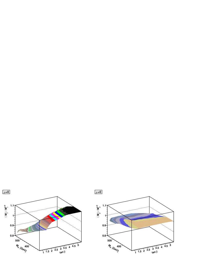
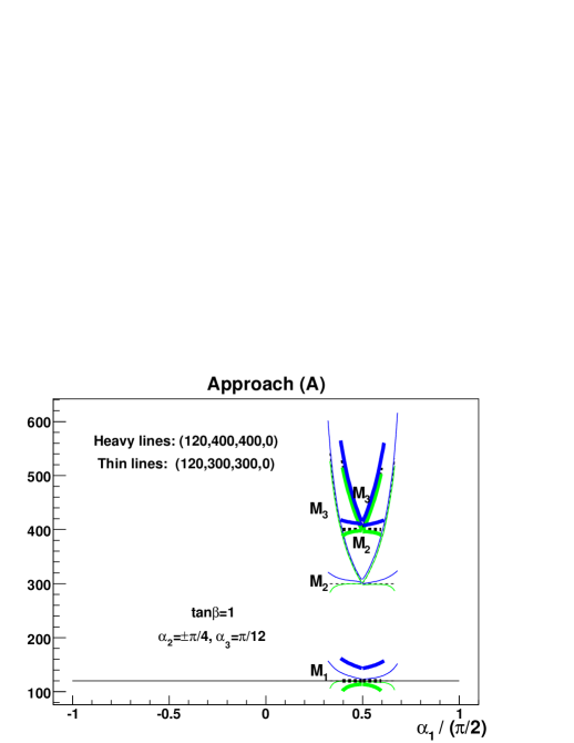
In Fig. 8 we show, for approach (A), the one-loop corrected Higgs boson masses, corresponding to the trilinear couplings studied in Fig. 1 (i.e., with α2subscript𝛼2\alpha_{2} and α3subscript𝛼3\alpha_{3} held fixed), due to the one-loop radiative corrections discussed above. The superscript ‘LO’ here denotes lowest-order values. The Higgs boson masses are determined as eigenvalues of the matrix (IV.2), evaluated for η1=η2=η3=0subscript𝜂1subscript𝜂2subscript𝜂30\eta_{1}=\eta_{2}=\eta_{3}=0. The full η𝜂\eta-dependence, to be discussed in the next section, will however be required for evaluating the one-loop trilinear Higgs couplings.
Refer to caption
Figure 8: One-loop Higgs masses M1subscript𝑀1M_{1}, M2subscript𝑀2M_{2} and M3subscript𝑀3M_{3} (in units of GeV) plotted as functions of α1subscript𝛼1\alpha_{1}, with α2=±π/4subscript𝛼2plus-or-minus𝜋4\alpha_{2}=\pm\pi/4, both with α3=π/12subscript𝛼3𝜋12\alpha_{3}=\pi/12. The lowest-order Higgs masses are M1LO=120GeVsuperscriptsubscript𝑀1LO120GeVM_{1}^{\text{LO}}=120~{}\text{GeV}, with M2LO=MH±LO=300GeVsuperscriptsubscript𝑀2LOsuperscriptsubscript𝑀superscript𝐻plus-or-minusLO300GeVM_{2}^{\text{LO}}=M_{H^{\pm}}^{\text{LO}}=300~{}\text{GeV} (thin lines), and M2LO=MH±LO=400GeVsuperscriptsubscript𝑀2LOsuperscriptsubscript𝑀superscript𝐻plus-or-minusLO400GeVM_{2}^{\text{LO}}=M_{H^{\pm}}^{\text{LO}}=400~{}\text{GeV} (heavy lines). Here μ=0𝜇0\mu=0 and tanβ=1𝛽1\tan\beta=1. Dashed lines refer to tree-level values, whereas green and blue lines refer to one-loop-corrected results, with the scale parameter Q=2M1LO𝑄2superscriptsubscript𝑀1LOQ=2M_{1}^{\text{LO}} and Q=500GeV𝑄500GeVQ=500~{}\text{GeV}, respectively.

The following points are worth noting here: (i) The tree-level value of M3subscript𝑀3M_{3}, namely M3LOsuperscriptsubscript𝑀3LOM_{3}^{\text{LO}}, has a strong dependence on α1subscript𝛼1\alpha_{1}. This is a consequence of keeping M1LOsuperscriptsubscript𝑀1LOM_{1}^{\text{LO}}, M2LOsuperscriptsubscript𝑀2LOM_{2}^{\text{LO}}, α2subscript𝛼2\alpha_{2} and α3subscript𝛼3\alpha_{3} fixed. (ii) The one-loop corrections have a significant dependence on the scale at which they are evaluated, as is illustrated by comparing the values of the Higgs boson masses at two different values of Q2superscript𝑄2Q^{2}. (iii) The one-loop correction to the Higgs boson mass can be either positive or negative. (iv) At some of the boundaries of the allowed parameter space, these one-loop corrections become large.

The reason for the strong variation of M3subscript𝑀3M_{3} at the edges of the allowed parameter space can be found from an inspection of the different origin of such edges. These can be described as follows:

  1. 1.

    In approach (A), at tree level, (M3LO)2superscriptsuperscriptsubscript𝑀3LO2(M_{3}^{\text{LO}})^{2} is determined as a rational fraction, where the numerator is linear in (M1LO)2superscriptsuperscriptsubscript𝑀1LO2(M_{1}^{\text{LO}})^{2} and (M2LO)2superscriptsuperscriptsubscript𝑀2LO2(M_{2}^{\text{LO}})^{2} (multiplying rotation matrix elements and tanβ𝛽\tan\beta), whereas the denominator is a linear function in rotation matrix elements and tanβ𝛽\tan\beta (For an explicit formula, see Eq. (4.16) of Ref. Khater:2003wq .). For critical values of the rotation matrix elements, e.g., when R31=R32tanβsubscript𝑅31subscript𝑅32𝛽R_{31}=R_{32}\tan\beta, the denominator will pass through zero. At such points, M3LOsuperscriptsubscript𝑀3LOM_{3}^{\text{LO}} diverges, and the allowed parameter space terminates.

  2. 2.

    In approach (A), M32superscriptsubscript𝑀32M_{3}^{2} may at some critical values of the rotation matrix elements become equal to M22superscriptsubscript𝑀22M_{2}^{2}. This happens when either R13=0subscript𝑅130R_{13}=0 or R12tanβ=R11subscript𝑅12𝛽subscript𝑅11R_{12}\tan\beta=R_{11} Khater:2003wq . In the former case we have α2=0subscript𝛼20\alpha_{2}=0 (α1subscript𝛼1\alpha_{1} and α3subscript𝛼3\alpha_{3} being arbitrary), whereas in the latter we have tanβ=cotα1𝛽subscript𝛼1\tan\beta=\cot\alpha_{1} (α2subscript𝛼2\alpha_{2} and α3subscript𝛼3\alpha_{3} being arbitrary).

  3. 3.

    Positivity may break down.

  4. 4.

    Perturbative unitarity may break down.

  5. 5.

    Parameter space may be truncated by some experimental constraint.

The first two of these cases are illustrated in Fig. 8. We actually exclude, as ‘unphysical’, regions where M1<100GeVsubscript𝑀1100GeVM_{1}<100~{}\text{GeV} (for M1LO=120GeVsuperscriptsubscript𝑀1LO120GeVM_{1}^{\text{LO}}=120~{}\text{GeV}) and where either M3LO>2M2LOsuperscriptsubscript𝑀3LO2superscriptsubscript𝑀2LOM_{3}^{\text{LO}}>2M_{2}^{\text{LO}} or M3>2M2subscript𝑀32subscript𝑀2M_{3}>2M_{2}.

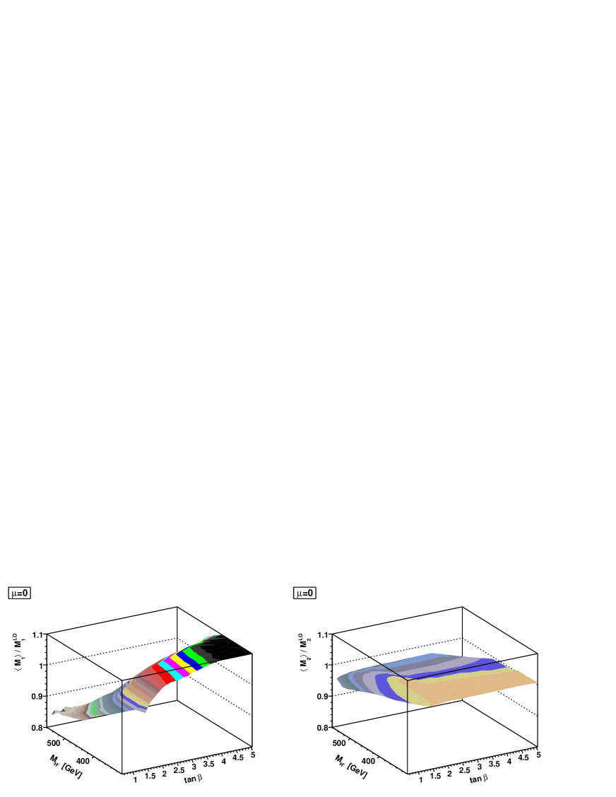
Refer to caption
Figure 9: One-loop multiplicative mass correction for tree-level mass parameters M1=120GeVsubscript𝑀1120GeVM_{1}=120~{}\text{GeV}, M2=300GeVsubscript𝑀2300GeVM_{2}=300~{}\text{GeV} and μ=0𝜇0\mu=0.

For approach (A), positivity is expressed in terms of simple inequalities, whereas for approach (B), with α6subscript𝛼6\alpha_{6} and α7subscript𝛼7\alpha_{7} non-zero, an involved numerical test is required ElKaffas:2006nt . Perturbative unitarity in the Higgs–Higgs scattering sector tends to truncate high values of tanβ𝛽\tan\beta, unless μ𝜇\mu is large (comparable to M2subscript𝑀2M_{2}) ElKaffas:2007rq .

Having described the radiative corrections to the Higgs masses, we next show in Fig. 9 typical one-loop multiplicative mass corrections, i.e., M1/M1LOsubscript𝑀1superscriptsubscript𝑀1LOM_{1}/M_{1}^{\text{LO}} and M2/M2LOsubscript𝑀2superscriptsubscript𝑀2LOM_{2}/M_{2}^{\text{LO}} for the case M1LO=120GeVsuperscriptsubscript𝑀1LO120GeVM_{1}^{\text{LO}}=120~{}\text{GeV}, M2LO=300GeVsuperscriptsubscript𝑀2LO300GeVM_{2}^{\text{LO}}=300~{}\text{GeV}, and μ=0𝜇0\mu=0. (This will be discussed in more detail in Sec. VII.) The renormalization scale has been chosen as Q2=(2M1LO)2superscript𝑄2superscript2superscriptsubscript𝑀1LO2Q^{2}=(2M_{1}^{\text{LO}})^{2}. As in Section III, an average over allowed points in 𝜶𝜶{\boldsymbol{\alpha}} has been performed.

For M1subscript𝑀1M_{1}, the loop correction is (for Q2=(2M1LO)2superscript𝑄2superscript2superscriptsubscript𝑀1LO2Q^{2}=(2M_{1}^{\text{LO}})^{2}) negative at low values of tanβ𝛽\tan\beta, whereas it is positive for higher values. For M2subscript𝑀2M_{2}, on the other hand, the correction is smaller, and has no strong dependence on tanβ𝛽\tan\beta. The negative correction for M1subscript𝑀1M_{1} is different from the MSSM, where the one-loop corrections, dominated by the top-quark (squark) contribution, is positive. Here, it is the Higgs sector which dominates, and this contribution has the opposite sign, because of the bosonic nature of the contributing particles in the loop. In actual practice the situation is more complicated, since different Higgs fields may contribute with different signs, depending on how the mass of the respective Higgs boson compares with the scale Q𝑄Q.

In view of the fact that the one-loop correction to M1subscript𝑀1M_{1} can be significant, and negative, we impose the constraint of LEP2 non-discovery of a Higgs boson on the one-loop corrected lightest Higgs boson mass. Higgs boson masses below the “magic” 114.4 GeV value are of course allowed, provided the coupling to the Z𝑍Z and bb¯𝑏¯𝑏b\bar{b} (or τ𝜏\tau pairs) are suppressed.

Treating the loop corrections as a perturbation, we have here imposed the theoretical and experimental constraints on the tree-level parameters. We note that at low values of tanβ𝛽\tan\beta, the mass of the lightest Higgs boson, M1subscript𝑀1M_{1}, may be considerably reduced. When we proceed to study the trilinear couplings, we shall therefore impose the LEP2 non-discovery constraint on the loop-corrected mass, M1subscript𝑀1M_{1}. For a higher scale parameter, though, the mass may increase also at low values of tanβ𝛽\tan\beta.

V One-loop Corrections to the Trilinear Higgs Couplings

The one-loop corrected trilinear Higgs couplings are given by the third order derivatives of the one-loop effective potential with respect to different fields. We shall separately consider the contributions to the potential from the neutral Higgs fields, the charged Higgs fields and the top quark fields. We start the calculation by evaluating the derivatives with respect to the weak fields, which can then be converted to derivatives with respect to the fields corresponding to the mass eigenstates with the help of Eq. (24).

The starting point of the calculation of the one-loop corrections to the trilinear Higgs couplings is the expression (IV.1). From this we obtain the one-loop radiative corrections to the trilinear Higgs couplings due to neutral Higgs bosons as

3ΔVneutral Higgsηiηjηk=132π2=13[1M2M2ηiM2ηjM2ηk\displaystyle\frac{\partial^{3}\Delta V_{\text{neutral Higgs}}}{\partial\eta_{i}\partial\eta_{j}\partial\eta_{k}}=\frac{1}{32\pi^{2}}\sum_{\ell=1}^{3}\biggl{[}\frac{1}{M_{\ell}^{2}}\frac{\partial M_{\ell}^{2}}{\partial\eta_{i}}\frac{\partial M_{\ell}^{2}}{\partial\eta_{j}}\frac{\partial M_{\ell}^{2}}{\partial\eta_{k}}
+logM2Q2(2M2ηiηjM2ηk+2M2ηjηkM2ηi\displaystyle\quad+\log\frac{M_{\ell}^{2}}{Q^{2}}\biggl{(}\frac{\partial^{2}M_{\ell}^{2}}{\partial\eta_{i}\partial\eta_{j}}\frac{\partial M_{\ell}^{2}}{\partial\eta_{k}}+\frac{\partial^{2}M_{\ell}^{2}}{\partial\eta_{j}\partial\eta_{k}}\frac{\partial M_{\ell}^{2}}{\partial\eta_{i}}
+2M2ηkηiM2ηj)+M2(logM2Q21)3M2ηiηjηk].\displaystyle\quad+\frac{\partial^{2}M_{\ell}^{2}}{\partial\eta_{k}\partial\eta_{i}}\frac{\partial M_{\ell}^{2}}{\partial\eta_{j}}\biggr{)}+M_{\ell}^{2}\biggl{(}\log\frac{M_{\ell}^{2}}{Q^{2}}-1\biggr{)}\frac{\partial^{3}M_{\ell}^{2}}{\partial\eta_{i}\partial\eta_{j}\partial\eta_{k}}\biggr{]}. (60)

The derivatives of squared masses with respect to the weak fields ηisubscript𝜂𝑖\eta_{i} in (V) are evaluated and discussed in Appendix C.

To find one-loop charged Higgs boson correction to the trilinear couplings, we start with field-dependent squared masses, MH±2(η1,η2,η3)superscriptsubscript𝑀superscript𝐻plus-or-minus2subscript𝜂1subscript𝜂2subscript𝜂3M_{H^{\pm}}^{2}(\eta_{1},\eta_{2},\eta_{3}), for the charged Higgs boson. Noting that the potential is a function of masses, i.e., ΔVcharged Higgs=ΔV(η1,η2,η3)Δsubscript𝑉charged HiggsΔ𝑉subscript𝜂1subscript𝜂2subscript𝜂3\Delta V_{\text{charged Higgs}}=\Delta V(\eta_{1},\eta_{2},\eta_{3}), we obtain

3ΔVcharged Higgsηiηjηk=116π2[1MH±2MH±2ηiMH±2ηjMH±2ηk\displaystyle\frac{\partial^{3}\Delta V_{\text{charged Higgs}}}{\partial\eta_{i}\partial\eta_{j}\partial\eta_{k}}=\frac{1}{16\pi^{2}}\biggl{[}\frac{1}{M_{H^{\pm}}^{2}}\frac{\partial M_{H^{\pm}}^{2}}{\partial\eta_{i}}\frac{\partial M_{H^{\pm}}^{2}}{\partial\eta_{j}}\frac{\partial M_{H^{\pm}}^{2}}{\partial\eta_{k}}
+logMH±2Q2(2MH±2ηiηjMH±2ηk+2MH±2ηjηkMH±2ηi\displaystyle\quad+\log\frac{M_{H^{\pm}}^{2}}{Q^{2}}\biggl{(}\frac{\partial^{2}M_{H^{\pm}}^{2}}{\partial\eta_{i}\partial\eta_{j}}\frac{\partial M_{H^{\pm}}^{2}}{\partial\eta_{k}}+\frac{\partial^{2}M_{H^{\pm}}^{2}}{\partial\eta_{j}\partial\eta_{k}}\frac{\partial M_{H^{\pm}}^{2}}{\partial\eta_{i}}
+2MH±2ηkηiMH±2ηj)].\displaystyle\quad+\frac{\partial^{2}M_{H^{\pm}}^{2}}{\partial\eta_{k}\partial\eta_{i}}\frac{\partial M_{H^{\pm}}^{2}}{\partial\eta_{j}}\biggr{)}\biggr{]}. (61)

For the one-loop corrections arising from the top-quark, we note that in Model II (which we consider) the up-type quarks couple only to Φ2subscriptΦ2\Phi_{2} (and not to Φ1subscriptΦ1\Phi_{1}). Thus, the one-loop contribution due to top quark affects only the fields η2subscript𝜂2\eta_{2}. We can then write

3ΔVtopηiηjηk=12π2mt4v23logmt2Q2δi2δj2δk2.superscript3Δsubscript𝑉topsubscript𝜂𝑖subscript𝜂𝑗subscript𝜂𝑘12superscript𝜋2superscriptsubscript𝑚𝑡4superscriptsubscript𝑣23superscriptsubscript𝑚𝑡2superscript𝑄2subscript𝛿𝑖2subscript𝛿𝑗2subscript𝛿𝑘2\frac{\partial^{3}\Delta V_{\text{top}}}{\partial\eta_{i}\partial\eta_{j}\partial\eta_{k}}=-\frac{12}{\pi^{2}}\frac{m_{t}^{4}}{v_{2}^{3}}\log\frac{m_{t}^{2}}{Q^{2}}\,\delta_{i2}\delta_{j2}\delta_{k2}. (62)

VI Quantitative results for trilinear Higgs couplings

We have seen that the lowest order trilinear couplings are highly dependent on the details of the two Higgs doublet model. This sensitivity on the details of the model is actually enhanced when we take into account the one-loop corrections to the Higgs potential. The loop corrections to the trilinear couplings can vary strongly with the parameters of the model, and also have a considerable dependence on the scale Q2superscript𝑄2Q^{2} used in Eqs. (V)–(62).

VI.1 Different contributions

For fixed values of α2subscript𝛼2\alpha_{2} and α3subscript𝛼3\alpha_{3}, as in Fig. 1, we show in Fig. 10 the ratio of the one-loop corrected trilinear Higgs coupling λ111subscript𝜆111\lambda_{111} and the corresponding tree-level coupling. This ratio is highly dependent on α1subscript𝛼1\alpha_{1} (as is the coupling itself).

Refer to caption
Figure 10: Contributions to the trilinear coupling ratio ξ1subscript𝜉1\xi_{1} plotted as functions of α1subscript𝛼1\alpha_{1}, for α2=±π/4subscript𝛼2plus-or-minus𝜋4\alpha_{2}=\pm\pi/4, both with α3=π/12subscript𝛼3𝜋12\alpha_{3}=\pi/12. The Higgs mass and parameters are as in Fig. 1. The scale parameter is Q=2M1LO𝑄2superscriptsubscript𝑀1LOQ=2M_{1}^{\text{LO}}. The full correction is shown by the upper, heavy, black lines, whereas partial contributions from neutral and charged Higgs bosons, as well as from top quarks, are shown by the thin, red, green and blue lines.

As compared with the one-loop corrections to the masses, the corrections to the trilinear couplings are relatively much larger. The following two points are worth noting: (i) Most of the one-loop contribution comes from the neutral-Higgs term, Eq. (V) (red lines labeled “H1,H2,H3subscript𝐻1subscript𝐻2subscript𝐻3H_{1},H_{2},H_{3}”). (ii) The correction can be very large at the boundary of the physically allowed region (in this case, in α1subscript𝛼1\alpha_{1}). These regions of very large corrections, which are excluded from averages over 𝜶𝜶{\boldsymbol{\alpha}}, will be discussed further in the following.

In approach (A), when we scan over the values of 𝜶𝜶{\boldsymbol{\alpha}}, there are regions where M3subscript𝑀3M_{3} gets very close to M2subscript𝑀2M_{2}. From Ref. Khater:2003wq , we see that (at tree level) this happens when (i) α20subscript𝛼20\alpha_{2}\to 0 or (ii) tanβcotα1𝛽subscript𝛼1\tan\beta\to\cot\alpha_{1}, or (iii) α2±π/2subscript𝛼2plus-or-minus𝜋2\alpha_{2}\to\pm\pi/2. Case (ii) occurs for tanβ=1𝛽1\tan\beta=1 and α1=π/4subscript𝛼1𝜋4\alpha_{1}=\pi/4. In this region, the trilinear coupling tends to get very large. This is clearly a region of parameter space where the present approach breaks down. In the notation of Appendix C [see Eq. (C.1)], we see that two roots merge (M3M2subscript𝑀3subscript𝑀2M_{3}\to M_{2}) when the complex phases of s1subscript𝑠1s_{1} and s2subscript𝑠2s_{2} differ by 2π/32𝜋32\pi/3. Near such points, the derivatives of s1subscript𝑠1s_{1} and s2subscript𝑠2s_{2} with respect to a𝑎a and b𝑏b, particularly the second and third-order ones, tend to get very large. Actually, such points have been removed from the following figures, and we impose a cut when scanning over 𝜶𝜶{\boldsymbol{\alpha}} in Sec. VI.4:

min{(M3LOM2LO),(M3M2)}>5GeV.superscriptsubscript𝑀3LOsuperscriptsubscript𝑀2LOsubscript𝑀3subscript𝑀25GeV\min\{(M_{3}^{\text{LO}}-M_{2}^{\text{LO}}),(M_{3}-M_{2})\}>5~{}\text{GeV}. (63)

VI.2 Scale dependence

Just as in the case of one-loop corrections to the masses, we note a strong dependence of the trilinear couplings on the scale parameter that enters the effective potential. This scale plays a role somewhat analogous to the mass scale of superpartners in the effective-potential approach to the MSSM.
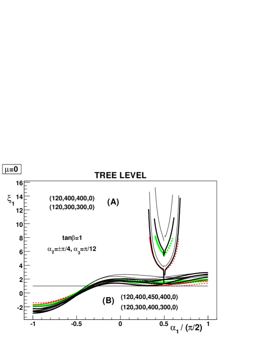
Refer to caption
Figure 11: Trilinear coupling ratio ξ1subscript𝜉1\xi_{1} [see Eq. (30)] as a function of α1subscript𝛼1\alpha_{1}. Colored lines refer to tree-level results (same color coding and parameters as in Fig. 1), black lines refer to loop-corrected results (thin: Q=2M1LO𝑄2superscriptsubscript𝑀1LOQ=2M_{1}^{\text{LO}}, heavy: Q=500GeV𝑄500GeVQ=500~{}\text{GeV}).

In Fig. 11 we study the one-loop corrected trilinear couplings, for both the approaches (A) and (B), and for two sets of Higgs masses within each approach (the same as in Fig. 1). We show how the one-loop corrections depend on the scale Q𝑄Q. For this purpose we have considered two timelike values of Q𝑄Q, namely, Q=2M1LO𝑄2superscriptsubscript𝑀1LOQ=2M_{1}^{\text{LO}} and Q=500GeV𝑄500GeVQ=500~{}\text{GeV}. As in the case of Fig. 10, we see that in approach (A), the couplings tend to get large near the boundary of the allowed parameter space. (Near α1=π/4subscript𝛼1𝜋4\alpha_{1}=\pi/4, we notice the irregular behavior discussed in Sec. VI.1, when M3M2subscript𝑀3subscript𝑀2M_{3}\to M_{2}.)

The dependence on the scale is rather involved, but there is a tendency that a lower scale gives a larger correction. This is rather clear in the upper part of the figure, which is a plot for approach (A). For approach (B), however, we have not labeled the individual curves, the main point being to show that there is a considerable uncertainty related to the choice of scale in both approaches.

VI.3 Decoupling

In the context of the trilinear Higgs coupling, decoupling would imply that the self-coupling of the light Higgs boson could be expressed in terms of its mass, as in the Standard Model. This was indeed found to hold for the MSSM, if the mass is taken to be the loop-corrected one Hollik:2001px ; Dobado:2002jz .
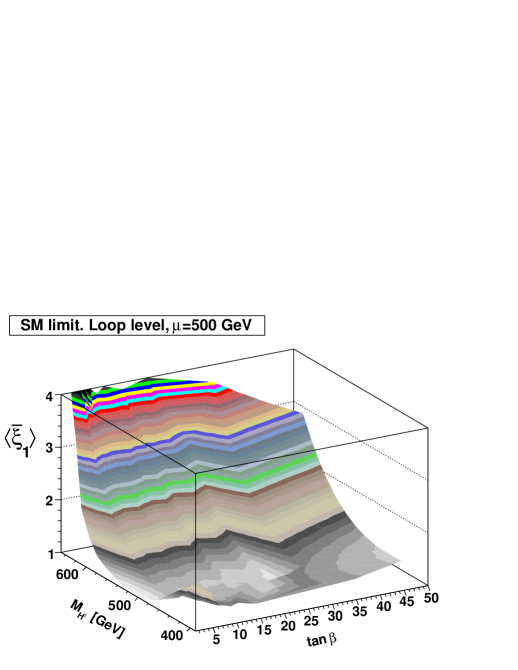
Refer to caption
Figure 12: Trilinear coupling ratio ξ¯1delimited-⟨⟩subscript¯𝜉1\langle\bar{\xi}_{1}\rangle as defined by Eq. (64). Different quantities in approach (A) with M1LO=120GeVsuperscriptsubscript𝑀1LO120GeVM_{1}^{\text{LO}}=120~{}\text{GeV}, M2LO=μ=500GeVsuperscriptsubscript𝑀2LO𝜇500GeVM_{2}^{\text{LO}}=\mu=500~{}\text{GeV}, and Q=2M1LO𝑄2superscriptsubscript𝑀1LOQ=2M_{1}^{\text{LO}}. The ratio ξ¯11similar-to-or-equalsdelimited-⟨⟩subscript¯𝜉11\langle\bar{\xi}_{1}\rangle\simeq 1 demonstrates approximate decoupling for M2=μMH±subscript𝑀2𝜇similar-tosubscript𝑀superscript𝐻plus-or-minusM_{2}=\mu\sim M_{H^{\pm}}.

In order to discuss decoupling in the 2HDM, we first need to define, as a reference, a Standard-Model-like limit by imposing the tree-level constraint (33), together with Eq. (44). The SM-like nature of this limit may be extended to the loop level, if in the loop corrections (IV.1) we include only the contributions of the lightest neutral Higgs boson H1subscript𝐻1H_{1} and the top quark. Within this framework, we may then study decoupling, by defining the ratio, analogous to (43):

ξ¯1=λ111fullλ111SM,delimited-⟨⟩subscript¯𝜉1delimited-⟨⟩superscriptsubscript𝜆111fulldelimited-⟨⟩superscriptsubscript𝜆111SM\langle\bar{\xi}_{1}\rangle=\frac{\langle\lambda_{111}^{\text{full}}\rangle}{\langle\lambda_{111}^{\text{SM}}\rangle}, (64)

where

  • λ111SMsuperscriptsubscript𝜆111SM\lambda_{111}^{\text{SM}} includes only loop corrections due to tt¯𝑡¯𝑡t\bar{t} and H1subscript𝐻1H_{1}, as would be the case in the SM.

  • λ111fullsuperscriptsubscript𝜆111full\lambda_{111}^{\text{full}} includes all one-loop corrections to the Higgs coupling in the two Higgs doublet model, i.e., also those due to H2subscript𝐻2H_{2}, H3subscript𝐻3H_{3} and H±superscript𝐻plus-or-minusH^{\pm}.

  • The averaging over α2subscript𝛼2\alpha_{2} and α3subscript𝛼3\alpha_{3} is constrained by Eq. (44) with α0=0.025×π/2subscript𝛼00.025𝜋2\alpha_{0}=0.025\times\pi/2, whereas α1subscript𝛼1\alpha_{1} is left unconstrained.

It should be noted that here we do not insist on a correspondence between the 2HDM and the MSSM, since this would require also α1βsimilar-to-or-equalssubscript𝛼1𝛽\alpha_{1}\simeq\beta.

If the ratio (64) were to come out as unity, it would be a signal for decoupling: the heavy Higgs bosons do not affect the coupling of the lightest one with itself. In Fig. 12, we display this ratio, for rather high values of M2LOsuperscriptsubscript𝑀2LOM_{2}^{\text{LO}} and μ𝜇\mu: M2LO=μ=500GeVsuperscriptsubscript𝑀2LO𝜇500GeVM_{2}^{\text{LO}}=\mu=500~{}\text{GeV}, subjecting all parameters to the general constraints discussed in Sec. III.1. For MH±M2similar-tosubscript𝑀superscript𝐻plus-or-minussubscript𝑀2M_{H^{\pm}}\sim M_{2}, the ratio (64) is indeed rather close to unity, but for larger values of MH±subscript𝑀superscript𝐻plus-or-minusM_{H^{\pm}}, it becomes significantly larger. In the region where ξ¯1<1.20<delimited-⟨⟩subscript¯𝜉11.20\langle\bar{\xi}_{1}\rangle\mathrel{\hbox to0.0pt{\raise 2.5pt\hbox{$<$}\hss}\lower 2.5pt\hbox{$\sim$}}1.20, we have also checked that M3M2<𝒪(40)GeVsubscript𝑀3subscript𝑀2𝒪40GeVM_{3}-M_{2}<{\cal O}(40)~{}\text{GeV}. Thus, in this region of the parameter space, decoupling holds at the loop level to about 10–20%. For larger values of MH±subscript𝑀superscript𝐻plus-or-minusM_{H^{\pm}}, however, where the model is still consistent, decoupling is strongly violated.
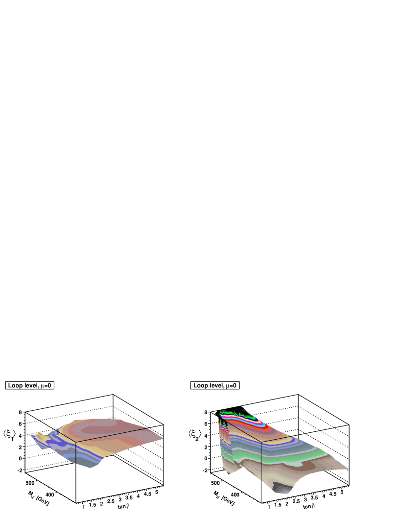
Refer to caption
Refer to caption
Refer to caption
Figure 13: Approach (A) with M1LO=120GeVsuperscriptsubscript𝑀1LO120GeVM_{1}^{\text{LO}}=120~{}\text{GeV}, M2LO=300GeVsuperscriptsubscript𝑀2LO300GeVM_{2}^{\text{LO}}=300~{}\text{GeV}, μ=0𝜇0\mu=0 and scale Q=2M1LO𝑄2superscriptsubscript𝑀1LOQ=2M_{1}^{\text{LO}}. Top panel: Trilinear coupling ratios ξ1delimited-⟨⟩subscript𝜉1\langle\xi_{1}\rangle and ξ2delimited-⟨⟩subscript𝜉2\langle\xi_{2}\rangle [see Eq. (43)]. Middle: one-loop multiplicative mass correction. Bottom: Variance of trilinear coupling ratios ξ1subscript𝜉1\xi_{1} and ξ2subscript𝜉2\xi_{2}.

The result displayed in Fig. 12 is quite stable under a change of α0subscript𝛼0\alpha_{0} from 0.025×π/20.025𝜋20.025\times\pi/2 to 0.05×π/20.05𝜋20.05\times\pi/2. However, the result depends on the choice of scale adopted for evaluating the one-loop potential. For example, for Q=500GeV𝑄500GeVQ=500~{}\text{GeV}, ξ¯1delimited-⟨⟩subscript¯𝜉1\langle\bar{\xi}_{1}\rangle differs significantly from unity. This is perhaps contrary to expectations, since log(M2LO/Q)superscriptsubscript𝑀2LO𝑄\log(M_{2}^{\text{LO}}/Q) then vanishes. However, we recall that (i) the one-loop potential also contains non-logarithmic terms, and (ii) the one-loop potential modifies the minimization conditions, i.e., its contribution shifts the values of the soft parameters m112superscriptsubscript𝑚112m_{11}^{2} and m222superscriptsubscript𝑚222m_{22}^{2} of the tree level potential.

In the 2HDM, in contrast to the MSSM, the decoupling cannot be exact. The reason is obvious: the heavy fields that we would like to neglect, are all bosonic, and thus all contribute with the same sign to the potential. Furthermore, even if we choose the scale Q𝑄Q such that the logarithms vanish, there would still be the non-logarithmic remainders.

The question of decoupling can be illustrated by the behavior of the ρ𝜌\rho parameter, which gets contributions from all pairs of Higgs bosons. These contributions vanish for equal masses, but are large when the masses are very different.

In the limit of no CP violation, custodial symmetry Weinberg:1972fn would imply MH±=Mjsubscript𝑀superscript𝐻plus-or-minussubscript𝑀𝑗M_{H^{\pm}}=M_{j}, where Mjsubscript𝑀𝑗M_{j} is either the mass of the CP odd (A𝐴A) or a CP even (H𝐻H) Higgs particle Gerard:2007kn . In the case that MH±=Asubscript𝑀superscript𝐻plus-or-minus𝐴M_{H^{\pm}}=A, orthogonality of the even-sector mixing matrix would protect the ΔρΔ𝜌\Delta\rho parameter from large corrections. In the present case of CP violation, a higher degeneracy is required, M2=M3=MH±subscript𝑀2subscript𝑀3subscript𝑀superscript𝐻plus-or-minusM_{2}=M_{3}=M_{H^{\pm}}, in order to avoid large contributions to ΔρΔ𝜌\Delta\rho. Since this is in general not satisfied, the experimental constraints on ΔρΔ𝜌\Delta\rho severely constrain the allowed parameter space WahabElKaffas:2007xd , and there is no decoupling.
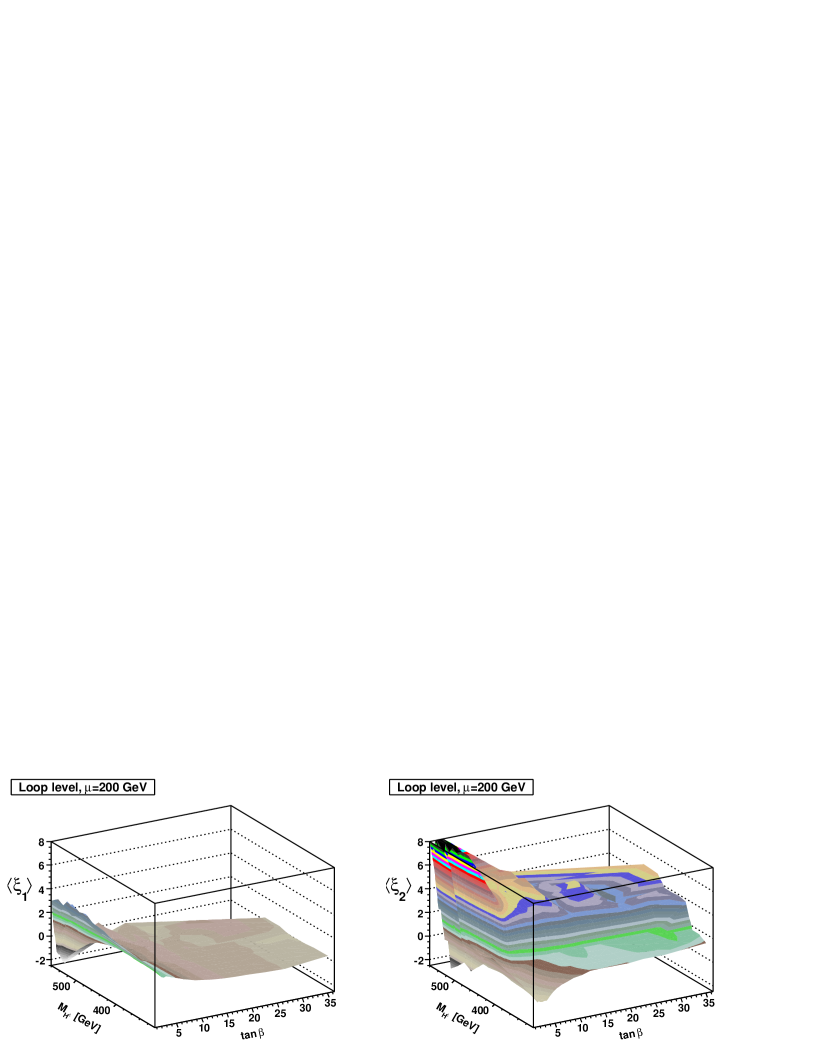
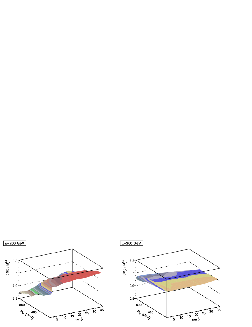
Refer to caption
Refer to caption
Refer to caption
Figure 14: Same as Fig. 13, but with μ=200GeV𝜇200GeV\mu=200~{}\text{GeV}.

VI.4 The general case

After this exploratory discussion, we are now ready to scan and average over the full range of 𝜶𝜶{\boldsymbol{\alpha}}, compatible with theoretical and experimental constraints on the model, as was done at tree level in Sec. III.1. Figs. 13 and 14 are plotted for approach (A) with M1LO=120GeVsuperscriptsubscript𝑀1LO120GeVM_{1}^{\text{LO}}=120~{}\text{GeV}, M2LO=300GeVsuperscriptsubscript𝑀2LO300GeVM_{2}^{\text{LO}}=300~{}\text{GeV}, μ=0𝜇0\mu=0 (Fig. 13), μ=200GeV𝜇200GeV\mu=200~{}\text{GeV} (Fig. 14) and with scale Q=2M1LO𝑄2superscriptsubscript𝑀1LOQ=2M_{1}^{\text{LO}} in both cases.

In these figures, we show the ratios ξ1delimited-⟨⟩subscript𝜉1\langle\xi_{1}\rangle and ξ2delimited-⟨⟩subscript𝜉2\langle\xi_{2}\rangle of trilinear couplings in the top panels. The middle panels are devoted to the loop-induced corrections to the masses M1subscript𝑀1M_{1} and M2subscript𝑀2M_{2}, whereas the bottom panels show the variance associated with the averaging of ξ1subscript𝜉1\xi_{1} and ξ2subscript𝜉2\xi_{2} over the 𝜶𝜶{\boldsymbol{\alpha}} parameter space.

An important difference between the two cases presented in these figures is the range in tanβ𝛽\tan\beta. As already discussed, for a low value of μ𝜇\mu, the high values of tanβ𝛽\tan\beta would lead to a model that would violate unitarity, and are, therefore, excluded ElKaffas:2006nt .

Comparing the top panels of Figs. 13 and 14 with the corresponding tree-level resuls shown in Fig. 3, we note the following: (i) The overall shape in the tanβ𝛽\tan\betaMH±subscript𝑀superscript𝐻plus-or-minusM_{H^{\pm}} plane is similar. (ii) The loop-corrected couplings are somewhat larger, after averaging over 𝜶𝜶\boldsymbol{\alpha}, in analogy with the results shown in Fig. 11 for α2subscript𝛼2\alpha_{2} and α3subscript𝛼3\alpha_{3} fixed.

The center panel of Fig. 13 is rather similar to Fig. 9, the only difference being that here the LEP2 constraint is imposed at the loop level. Focusing first on the loop corrections to M1subscript𝑀1M_{1}, and comparing the mass correction at the two different values of μ𝜇\mu, we note that the case μ=0𝜇0\mu=0 gives a larger reduction at low values of tanβ𝛽\tan\beta and a larger increase at high values of tanβ𝛽\tan\beta. For M2subscript𝑀2M_{2}, on the other hand, the loop correction has only a rather weak dependence on tanβ𝛽\tan\beta (and MH±subscript𝑀superscript𝐻plus-or-minusM_{H^{\pm}}). For a higher value of the scale Q𝑄Q, however, the loop correction to M1subscript𝑀1M_{1} may be positive also at low values of tanβ𝛽\tan\beta.

The trilinear couplings represented in these figures, are of course not physical, they are instead “typical values”, obtained by an averaging over the angles of the mixing matrix R𝑅R that diagonalizes the mass-squared matrix. As discussed above, the variation over the 𝜶𝜶{\boldsymbol{\alpha}} parameter space can be considerable, as illustrated by the variance shown in the bottom panels.

A more detailed comparison reveals that the loop corrections are most important for low values of low-tanβ𝛽\tan\beta. This is particularly so in the case of ξ2delimited-⟨⟩subscript𝜉2\langle\xi_{2}\rangle, where the variance is also quite large. This is in part caused by the ill-defined limit M3M2subscript𝑀3subscript𝑀2M_{3}\to M_{2} (α20subscript𝛼20\alpha_{2}\to 0) discussed above. [Actually, at high values of MH±subscript𝑀superscript𝐻plus-or-minusM_{H^{\pm}}, the ξ2delimited-⟨⟩subscript𝜉2\langle\xi_{2}\rangle plots are truncated at the top.]

Refer to caption
Refer to caption
Figure 15: Similar to the upper panels of Figs. 13 and 14, but for μ=500GeV𝜇500GeV\mu=500~{}\text{GeV}. Upper panels: M2LO=300GeVsuperscriptsubscript𝑀2LO300GeVM_{2}^{\text{LO}}=300~{}\text{GeV}; lower panels: M2LO=500GeVsuperscriptsubscript𝑀2LO500GeVM_{2}^{\text{LO}}=500~{}\text{GeV}. Note that the scales are different from those in the earlier figures.

The correlation between these trilinear couplings and the quartic couplings λisubscript𝜆𝑖\lambda_{i} of the tree-level potential or their averages, λidelimited-⟨⟩subscript𝜆𝑖\langle\lambda_{i}\rangle, is not very simple, but a couple of observations can be made. In Fig. 13, for μ=0𝜇0\mu=0 the enhancement at low values of tanβ𝛽\tan\beta is correlated with a corresponding enhancement of λ2delimited-⟨⟩subscript𝜆2\langle\lambda_{2}\rangle, whereas λ1delimited-⟨⟩subscript𝜆1\langle\lambda_{1}\rangle is large at high values of tanβ𝛽\tan\beta.

For the H1H1H1subscript𝐻1subscript𝐻1subscript𝐻1H_{1}H_{1}H_{1} coupling, represented by ξ1delimited-⟨⟩subscript𝜉1\langle\xi_{1}\rangle, we note that for μ=0𝜇0\mu=0 it is rather large for all values of tanβ𝛽\tan\beta and MH±subscript𝑀superscript𝐻plus-or-minusM_{H^{\pm}} where the model is consistent, whereas for μ=200GeV𝜇200GeV\mu=200~{}\text{GeV} it falls to zero for large values of tanβ𝛽\tan\beta.

Finally, in Fig. 15 we show the behavior for somewhat higher value of the soft mass parameter, μ=500GeV𝜇500GeV\mu=500~{}\text{GeV}. We display the averages ξ1delimited-⟨⟩subscript𝜉1\langle\xi_{1}\rangle and ξ2delimited-⟨⟩subscript𝜉2\langle\xi_{2}\rangle for two values of M2LOsuperscriptsubscript𝑀2LOM_{2}^{\text{LO}}, 300 GeV (as was adopted in the earlier plots) and 500 GeV. Compared to the corresponding panels of Figs. 13 and 14, the present ones (for μ=500GeV𝜇500GeV\mu=500~{}\text{GeV}) are more smooth, and also somewhat different in magnitude.

VII Summary and Conclusions

The two Higgs doublet model is a viable extension of the Standard Model Higgs sector. Apart from having a richer structure of Higgs bosons and Higgs couplings, it can accommodate CP violation beyond that of the Kobayashi–Maskawa mechanism in the SM. In this paper we have studied in detail the trilinear couplings of the lightest Higgs boson of this model, including the CP violating effects. Our main objective has been to study the implications of CP violation for the trilinear couplings of the general two Higgs doublet model. We have discussed two different parametrizations of the general two Higgs doublet model, and imposed the constraints on the parameters of the model following from theoretical considerations and from different experiments. Tree-level unitarity, B𝐵B physics and ΔρΔ𝜌\Delta\rho are the most constraining ones for the parameters of the two Higgs doublet moddel with CP violation.

Within the allowed domain of the parameter space of the model, the trilinear couplings can have a very strong dependence on the neutral Higgs boson mixing angles. Because of this strong dependence of the trilinear couplings on the mixing angles, we have presented averages over the allowed ranges for these angles. Together with the variances, these show the range of trilinear couplings that can be expected in the two Higgs doublet model with CP violation.

There is a region of parameter space of the 2HDM, which we call “minimal CP violation,” which corresponds to the domain of parameters close to the Higgs sector of the CP-conserving minimal supersymmetric standard model. In much of this parameter space there is a considerable enhancement of the trilinear couplings of the two Higgs doublet model as compared with the corresponding trilinear coupling of the SM.

We have computed the radiative corrections to the masses of the Higgs bosons and the trilinear couplings in the one-loop effective potential approximation. The one-loop corrected mass of the lightest neutral Higgs boson can be modified by as much as 20%, whereas the heavier ones are less affected by the radiative corrections. The one-loop corrected trilinear couplings are typically enhanced by the loop effects, but so is the sensitivity to the neutral-sector mixing angles. A similar enhancement due to CP violating effects has also been found for the MSSM Dubinin:2002nx ; Philippov:2006th .

To a good approximation, decoupling holds in a limited range of parameters, where the model is close to the CP-conserving MSSM. In general, however, the heavier states also have a considerable impact on the properties of the lightest Higgs boson. In this sense there is no decoupling in the two Higgs doublet model with CP violation.

VIII Acknowledgements

The research of PO has been supported in part by the Research Council of Norway. The work of PNP is supported by the Board of Research in Nuclear Sciences, India under project No. 2007/37/34/BRNS/1970. He would like to thank the the Abdus Salam ICTP, Trieste, and Department of Physics and Technology, University of Bergen for hospitality where part of this work was done. LS is grateful to Department of Physics and Technology, University of Bergen for its generous hospitality, where part of this work was done, and The Scientific and Technological Research Council of Turkey (TUBITAK) for financial support. It is a great pleasure for LS to thank Zekeriya Aydin and Dumus Ali Demir for useful discussions in the early stages of this work.

Appendix A Quartic couplings expressed in terms of masses

In the 2HDM, with Imλ50Imsubscript𝜆50{\rm Im\thinspace}\lambda_{5}\neq 0, the two masses M1subscript𝑀1M_{1} and M2subscript𝑀2M_{2}, together with 𝜶𝜶{\boldsymbol{\alpha}} and tanβ𝛽\tan\beta, determine M3subscript𝑀3M_{3}. The masses will also be related to the quartic couplings of the Higgs potential, via linear relations that can be unambiguously inverted. It is convenient to distinguish two cases, whether or not λ6subscript𝜆6\lambda_{6} and λ7subscript𝜆7\lambda_{7} are non-zero.

A.1 Approach (A), 𝝀𝟔=𝝀𝟕=𝟎subscript𝝀6subscript𝝀70\boldsymbol{\lambda_{6}=\lambda_{7}=0}

This case is referred to as approach (A) in the text. Providing also MH±subscript𝑀superscript𝐻plus-or-minusM_{H^{\pm}} and μ2superscript𝜇2\mu^{2}, in addition to M1subscript𝑀1M_{1}, M2subscript𝑀2M_{2} and 𝜶𝜶{\boldsymbol{\alpha}}, all the λ𝜆\lambda’s are determined as follows ElKaffas:2006nt ; ElKaffas:2007rq :

λ1subscript𝜆1\displaystyle\lambda_{1} =1cβ2v2[c12c22M12+(c1s2s3+s1c3)2M22\displaystyle=\frac{1}{c_{\beta}^{2}v^{2}}[c_{1}^{2}c_{2}^{2}M_{1}^{2}+(c_{1}s_{2}s_{3}+s_{1}c_{3})^{2}M_{2}^{2}
+(c1s2c3s1s3)2M32sβ2μ2],\displaystyle+(c_{1}s_{2}c_{3}-s_{1}s_{3})^{2}M_{3}^{2}-s_{\beta}^{2}\mu^{2}], (65)
λ2subscript𝜆2\displaystyle\lambda_{2} =1sβ2v2[s12c22M12+(c1c3s1s2s3)2M22\displaystyle=\frac{1}{s_{\beta}^{2}v^{2}}[s_{1}^{2}c_{2}^{2}M_{1}^{2}+(c_{1}c_{3}-s_{1}s_{2}s_{3})^{2}M_{2}^{2}
+(c1s3+s1s2c3)2M32cβ2μ2],\displaystyle+(c_{1}s_{3}+s_{1}s_{2}c_{3})^{2}M_{3}^{2}-c_{\beta}^{2}\mu^{2}], (66)
λ3subscript𝜆3\displaystyle\lambda_{3} =1cβsβv2{c1s1[c22M12+(s22s32c32)M22\displaystyle=\frac{1}{c_{\beta}s_{\beta}v^{2}}\{c_{1}s_{1}[c_{2}^{2}M_{1}^{2}+(s_{2}^{2}s_{3}^{2}-c_{3}^{2})M_{2}^{2}
+(s22c32s32)M32]+s2c3s3(c12s12)(M32M22)}\displaystyle+(s_{2}^{2}c_{3}^{2}-s_{3}^{2})M_{3}^{2}]+s_{2}c_{3}s_{3}(c_{1}^{2}-s_{1}^{2})(M_{3}^{2}-M_{2}^{2})\}
+\displaystyle+ 1v2[2MH±2μ2],1superscript𝑣2delimited-[]2superscriptsubscript𝑀superscript𝐻plus-or-minus2superscript𝜇2\displaystyle\frac{1}{v^{2}}[2M_{H^{\pm}}^{2}-\mu^{2}], (67)
λ4subscript𝜆4\displaystyle\lambda_{4} =1v2[s22M12+c22s32M22+c22c32M32+μ22MH±2],absent1superscript𝑣2delimited-[]superscriptsubscript𝑠22superscriptsubscript𝑀12superscriptsubscript𝑐22superscriptsubscript𝑠32superscriptsubscript𝑀22superscriptsubscript𝑐22superscriptsubscript𝑐32superscriptsubscript𝑀32superscript𝜇22superscriptsubscript𝑀superscript𝐻plus-or-minus2\displaystyle=\frac{1}{v^{2}}[s_{2}^{2}M_{1}^{2}+c_{2}^{2}s_{3}^{2}M_{2}^{2}+c_{2}^{2}c_{3}^{2}M_{3}^{2}+\mu^{2}-2M_{H^{\pm}}^{2}], (68)
Reλ5Resubscript𝜆5\displaystyle{\rm Re\thinspace}\lambda_{5} =1v2[s22M12c22s32M22c22c32M32+μ2],absent1superscript𝑣2delimited-[]superscriptsubscript𝑠22superscriptsubscript𝑀12superscriptsubscript𝑐22superscriptsubscript𝑠32superscriptsubscript𝑀22superscriptsubscript𝑐22superscriptsubscript𝑐32superscriptsubscript𝑀32superscript𝜇2\displaystyle=\frac{1}{v^{2}}[-s_{2}^{2}M_{1}^{2}-c_{2}^{2}s_{3}^{2}M_{2}^{2}-c_{2}^{2}c_{3}^{2}M_{3}^{2}+\mu^{2}], (69)
Imλ5Imsubscript𝜆5\displaystyle{\rm Im\thinspace}\lambda_{5} =1cβsβv2{cβ[c1c2s2M12c2s3(c1s2s3+s1c3)M22\displaystyle=\frac{-1}{c_{\beta}s_{\beta}v^{2}}\{c_{\beta}[c_{1}c_{2}s_{2}M_{1}^{2}-c_{2}s_{3}(c_{1}s_{2}s_{3}+s_{1}c_{3})M_{2}^{2}
+c2c3(s1s3c1s2c3)M32]+sβ[s1c2s2M12\displaystyle+c_{2}c_{3}(s_{1}s_{3}-c_{1}s_{2}c_{3})M_{3}^{2}]+s_{\beta}[s_{1}c_{2}s_{2}M_{1}^{2} (70)
+c2s3(c1c3s1s2s3)M22c2c3(c1s3+s1s2c3)M32]},\displaystyle+c_{2}s_{3}(c_{1}c_{3}\!-\!s_{1}s_{2}s_{3})M_{2}^{2}\!-\!c_{2}c_{3}(c_{1}s_{3}\!+\!s_{1}s_{2}c_{3})M_{3}^{2}]\},

where cβ=cosβsubscript𝑐𝛽𝛽c_{\beta}=\cos\beta, sβ=sinβsubscript𝑠𝛽𝛽s_{\beta}=\sin\beta.

While M32superscriptsubscript𝑀32M_{3}^{2} is given in terms of M12superscriptsubscript𝑀12M_{1}^{2}, M22superscriptsubscript𝑀22M_{2}^{2}, R𝑅R and tanβ𝛽\tan\beta, it is more transparent not to substitute for M32superscriptsubscript𝑀32M_{3}^{2} in the expressions (A.1)–(70). These equations are the analogues of those of Casalbuoni:1987cz for the CP-conserving 2HDM.

A.2 Approach (B), 𝝀𝟔𝟎subscript𝝀60\boldsymbol{\lambda_{6}\neq 0}, 𝝀𝟕𝟎subscript𝝀70\boldsymbol{\lambda_{7}\neq 0}

In this case, referred to as approach (B) in the text, we take M1subscript𝑀1M_{1}, M2subscript𝑀2M_{2}, M2subscript𝑀2M_{2}, 𝜶𝜶{\boldsymbol{\alpha}}, MH±subscript𝑀superscript𝐻plus-or-minusM_{H^{\pm}} and μ2superscript𝜇2\mu^{2}, together with Imλ5Imsubscript𝜆5{\rm Im\thinspace}\lambda_{5}, Reλ6Resubscript𝜆6{\rm Re\thinspace}\lambda_{6} and Reλ7Resubscript𝜆7{\rm Re\thinspace}\lambda_{7}, as the input. In order to keep the notation compact, it is convenient to introduce the following abbreviations:

Reλ345Resubscript𝜆345\displaystyle{\rm Re\thinspace}\lambda_{345} =λ3+λ4+Reλ5,absentsubscript𝜆3subscript𝜆4Resubscript𝜆5\displaystyle=\lambda_{3}+\lambda_{4}+{\rm Re\thinspace}\lambda_{5}, (71)
Reλ567Resubscript𝜆567\displaystyle{\rm Re\thinspace}\lambda_{567} =Reλ5+cotβReλ6+tanβReλ7.absentResubscript𝜆5𝛽Resubscript𝜆6𝛽Resubscript𝜆7\displaystyle={\rm Re\thinspace}\lambda_{5}+\cot\beta\,{\rm Re\thinspace}\lambda_{6}+\tan\beta\,{\rm Re\thinspace}\lambda_{7}. (72)

Then, the λ𝜆\lambda’s can be determined from the following relations:

λ1subscript𝜆1\displaystyle\lambda_{1} =1cβ2[112sβ2μ2v2sβ2cβ(3cβ2Reλ6sβ2Reλ7)],absent1superscriptsubscript𝑐𝛽2delimited-[]superscriptsubscript112superscriptsubscript𝑠𝛽2superscript𝜇2superscript𝑣2subscript𝑠𝛽2subscript𝑐𝛽3superscriptsubscript𝑐𝛽2Resubscript𝜆6superscriptsubscript𝑠𝛽2Resubscript𝜆7\displaystyle=\frac{1}{c_{\beta}^{2}}\biggl{[}\frac{{\cal M}_{11}^{2}-s_{\beta}^{2}\mu^{2}}{v^{2}}\!-\!\frac{s_{\beta}}{2c_{\beta}}(3c_{\beta}^{2}{\rm Re\thinspace}\lambda_{6}-s_{\beta}^{2}{\rm Re\thinspace}\lambda_{7})\biggr{]}, (73)
λ2subscript𝜆2\displaystyle\lambda_{2} =1sβ2[222cβ2μ2v2+cβ2sβ(cβ2Reλ63sβ2Reλ7)],absent1superscriptsubscript𝑠𝛽2delimited-[]superscriptsubscript222superscriptsubscript𝑐𝛽2superscript𝜇2superscript𝑣2subscript𝑐𝛽2subscript𝑠𝛽superscriptsubscript𝑐𝛽2Resubscript𝜆63superscriptsubscript𝑠𝛽2Resubscript𝜆7\displaystyle=\frac{1}{s_{\beta}^{2}}\biggl{[}\frac{{\cal M}_{22}^{2}-c_{\beta}^{2}\mu^{2}}{v^{2}}\!+\!\frac{c_{\beta}}{2s_{\beta}}(c_{\beta}^{2}{\rm Re\thinspace}\lambda_{6}-3s_{\beta}^{2}{\rm Re\thinspace}\lambda_{7})\biggr{]}, (74)
Reλ345Resubscript𝜆345\displaystyle{\rm Re\thinspace}\lambda_{345} =1cβsβ[cβsβμ2+122v2\displaystyle=\frac{1}{c_{\beta}s_{\beta}}\biggl{[}\frac{c_{\beta}s_{\beta}\mu^{2}+{\cal M}_{12}^{2}}{v^{2}}
32(cβ2Reλ6+sβ2Reλ7)],\displaystyle-\frac{3}{2}(c_{\beta}^{2}{\rm Re\thinspace}\lambda_{6}+s_{\beta}^{2}{\rm Re\thinspace}\lambda_{7})\biggr{]}, (75)
λ4subscript𝜆4\displaystyle\lambda_{4} =2v2[μ2MH±2]Reλ567,absent2superscript𝑣2delimited-[]superscript𝜇2superscriptsubscript𝑀superscript𝐻plus-or-minus2Resubscript𝜆567\displaystyle=\frac{2}{v^{2}}[\mu^{2}-M_{H^{\pm}}^{2}]-{\rm Re\thinspace}\lambda_{567}, (76)
Reλ5Resubscript𝜆5\displaystyle{\rm Re\thinspace}\lambda_{5} =μ2332v212cβsβ(cβ2Reλ6+sβ2Reλ7),absentsuperscript𝜇2superscriptsubscript332superscript𝑣212subscript𝑐𝛽subscript𝑠𝛽superscriptsubscript𝑐𝛽2Resubscript𝜆6superscriptsubscript𝑠𝛽2Resubscript𝜆7\displaystyle=\frac{\mu^{2}-{\cal M}_{33}^{2}}{v^{2}}-\frac{1}{2c_{\beta}s_{\beta}}(c_{\beta}^{2}{\rm Re\thinspace}\lambda_{6}+s_{\beta}^{2}{\rm Re\thinspace}\lambda_{7}), (77)
Imλ6Imsubscript𝜆6\displaystyle{\rm Im\thinspace}\lambda_{6} =12cβ[2132v2+sβImλ5],absent12subscript𝑐𝛽delimited-[]2superscriptsubscript132superscript𝑣2subscript𝑠𝛽Imsubscript𝜆5\displaystyle=-\frac{1}{2c_{\beta}}\biggl{[}\frac{2{\cal M}_{13}^{2}}{v^{2}}+s_{\beta}{\rm Im\thinspace}\lambda_{5}\biggr{]}, (78)
Imλ7Imsubscript𝜆7\displaystyle{\rm Im\thinspace}\lambda_{7} =12sβ[2232v2+cβImλ5].absent12subscript𝑠𝛽delimited-[]2superscriptsubscript232superscript𝑣2subscript𝑐𝛽Imsubscript𝜆5\displaystyle=-\frac{1}{2s_{\beta}}\biggl{[}\frac{2{\cal M}_{23}^{2}}{v^{2}}+c_{\beta}{\rm Im\thinspace}\lambda_{5}\biggr{]}. (79)

Invoking Eq. (15), the ij2superscriptsubscript𝑖𝑗2{\cal M}_{ij}^{2} can be expressed in terms of R𝑅R and the masses M1subscript𝑀1M_{1}, M2subscript𝑀2M_{2} and M3subscript𝑀3M_{3}.

Appendix B Trilinear coupling for some special cases

In order to get a feeling for the trilinear Higgs couplings of the 2HDM, we shall here explicitly write down the two trilinear couplings λ111subscript𝜆111\lambda_{111} and λ112subscript𝜆112\lambda_{112} for some special cases.

B.1 The trilinear coupling 𝝀𝟏𝟏𝟏subscript𝝀111\boldsymbol{\lambda_{111}}

We start by writing down Eq. (III.1) explicitly for {i,j,k}={1,1,1}𝑖𝑗𝑘111\{i,j,k\}=\{1,1,1\}:

λ111subscript𝜆111\displaystyle\lambda_{111} =mno=1,2,3R1mR1nR1oamnoabsentsuperscriptsubscriptformulae-sequence𝑚𝑛𝑜123subscript𝑅1𝑚subscript𝑅1𝑛subscript𝑅1𝑜subscript𝑎𝑚𝑛𝑜\displaystyle=\sum_{m\leq n\leq o=1,2,3}^{\ast}R_{1m}R_{1n}R_{1o}\,a_{mno}
=3!{R112[R11a111+R12a112+R13a113]\displaystyle=3!\{R_{11}^{2}[R_{11}\,a_{111}+R_{12}\,a_{112}+R_{13}\,a_{113}]
+R11[R122a122+R12R13a123+R132a133]subscript𝑅11delimited-[]superscriptsubscript𝑅122subscript𝑎122subscript𝑅12subscript𝑅13subscript𝑎123superscriptsubscript𝑅132subscript𝑎133\displaystyle+R_{11}[R_{12}^{2}a_{122}+R_{12}R_{13}\,a_{123}+R_{13}^{2}\,a_{133}]
+R12[R122a222+R12R13a223+R132a233]subscript𝑅12delimited-[]superscriptsubscript𝑅122subscript𝑎222subscript𝑅12subscript𝑅13subscript𝑎223superscriptsubscript𝑅132subscript𝑎233\displaystyle+R_{12}[R_{12}^{2}\,a_{222}+R_{12}R_{13}\,a_{223}+R_{13}^{2}\,a_{233}]
+R133a333},\displaystyle+R_{13}^{3}\,a_{333}\}, (80)

where the factor 3!33! is due to the fact that we here have couplings to three identical H1subscript𝐻1H_{1} fields. Substituting for the elements of the rotation matrix, Eq. (II.1), one obtains

λ111subscript𝜆111\displaystyle\lambda_{111} =3!{(c1c2)2[c1c2a111+s1c2a112+s2a113]\displaystyle=3!\{(c_{1}c_{2})^{2}[c_{1}c_{2}\,a_{111}+s_{1}c_{2}\,a_{112}+s_{2}\,a_{113}]
+c1c2[(s1c2)2a122+s1c2s2a123+s22a133]subscript𝑐1subscript𝑐2delimited-[]superscriptsubscript𝑠1subscript𝑐22subscript𝑎122subscript𝑠1subscript𝑐2subscript𝑠2subscript𝑎123superscriptsubscript𝑠22subscript𝑎133\displaystyle+c_{1}c_{2}[(s_{1}c_{2})^{2}\,a_{122}+s_{1}c_{2}s_{2}\,a_{123}+s_{2}^{2}\,a_{133}]
+s1c2[(s1c2)2a222+s1c2s2a223+s22a233]subscript𝑠1subscript𝑐2delimited-[]superscriptsubscript𝑠1subscript𝑐22subscript𝑎222subscript𝑠1subscript𝑐2subscript𝑠2subscript𝑎223superscriptsubscript𝑠22subscript𝑎233\displaystyle+s_{1}c_{2}[(s_{1}c_{2})^{2}\,a_{222}+s_{1}c_{2}s_{2}\,a_{223}+s_{2}^{2}\,a_{233}]
+s23a333}.\displaystyle+s_{2}^{3}\,a_{333}\}. (81)

Let us now consider the case of λ6=λ7=0subscript𝜆6subscript𝜆70\lambda_{6}=\lambda_{7}=0, and substitute for the coefficients amnosubscript𝑎𝑚𝑛𝑜a_{mno} from Eq. (III.1). In this case,

λ111subscript𝜆111\displaystyle\lambda_{111} =3{c1c2cβ(c12c22+s22sβ2)λ1+s1c2sβ(s12c22+s22cβ2)λ2\displaystyle=3\{c_{1}c_{2}c_{\beta}(c_{1}^{2}c_{2}^{2}+s_{2}^{2}s_{\beta}^{2})\lambda_{1}+s_{1}c_{2}s_{\beta}(s_{1}^{2}c_{2}^{2}+s_{2}^{2}c_{\beta}^{2})\lambda_{2}
2c2s22(c1cβ+s1sβ)Reλ3452subscript𝑐2superscriptsubscript𝑠22subscript𝑐1subscript𝑐𝛽subscript𝑠1subscript𝑠𝛽Resubscript𝜆345\displaystyle-2c_{2}s_{2}^{2}(c_{1}c_{\beta}+s_{1}s_{\beta}){\rm Re\thinspace}\lambda_{345}
s2[(c22s22)cβsβ+2c1s1c22]Imλ5}.\displaystyle-s_{2}[(c_{2}^{2}-s_{2}^{2})c_{\beta}s_{\beta}+2c_{1}s_{1}c_{2}^{2}]{\rm Im\thinspace}\lambda_{5}\}. (82)

In the limit of no CP violation, with H1subscript𝐻1H_{1} being odd, we have c2=0subscript𝑐20c_{2}=0 [see Eq. (16)], and the trilinear coupling simplifies further to

λ111=3s23cβsβImλ5,subscript𝜆1113superscriptsubscript𝑠23subscript𝑐𝛽subscript𝑠𝛽Imsubscript𝜆5\lambda_{111}=3s_{2}^{3}\,c_{\beta}s_{\beta}{\rm Im\thinspace}\lambda_{5}, (83)

with s2=±1subscript𝑠2plus-or-minus1s_{2}=\pm 1. Similarly, in the limit of no CP violation, with H3subscript𝐻3H_{3} being odd, we have s2=s3=0subscript𝑠2subscript𝑠30s_{2}=s_{3}=0, and obtain the simple expression given in Eq. (28), whereas the limit of no CP violation with H2subscript𝐻2H_{2} being odd, leads to no further simplification of the expression (B.1).

B.2 The trilinear coupling 𝝀𝟏𝟏𝟐subscript𝝀112\boldsymbol{\lambda_{112}}

We shall again first write Eq. (III.1) explicitly for {i,j,k}={1,1,2}𝑖𝑗𝑘112\{i,j,k\}=\{1,1,2\}:

λ112subscript𝜆112\displaystyle\lambda_{112} =mno=1,2,3RimRjnRkoamnoabsentsuperscriptsubscriptformulae-sequence𝑚𝑛𝑜123subscript𝑅superscript𝑖𝑚subscript𝑅superscript𝑗𝑛subscript𝑅superscript𝑘𝑜subscript𝑎𝑚𝑛𝑜\displaystyle=\sum_{m\leq n\leq o=1,2,3}^{\ast}R_{i^{\prime}m}R_{j^{\prime}n}R_{k^{\prime}o}\,a_{mno}
=2mno=1,2,3{R1mR1nR2o+R1mR2nR1o\displaystyle=2\sum_{m\leq n\leq o=1,2,3}\{R_{1m}R_{1n}R_{2o}+R_{1m}R_{2n}R_{1o}
+R2mR1nR1o}amno\displaystyle+R_{2m}R_{1n}R_{1o}\}a_{mno}
=2{3R112R21a111+R11(R11R22+2R12R21)a112\displaystyle=2\{3R_{11}^{2}R_{21}\,a_{111}+R_{11}(R_{11}R_{22}+2R_{12}R_{21})a_{112}
+R11(R11R23+2R13R21)a113subscript𝑅11subscript𝑅11subscript𝑅232subscript𝑅13subscript𝑅21subscript𝑎113\displaystyle+R_{11}(R_{11}R_{23}+2R_{13}R_{21})a_{113}
+R12(2R11R22+R12R21)a122subscript𝑅122subscript𝑅11subscript𝑅22subscript𝑅12subscript𝑅21subscript𝑎122\displaystyle+R_{12}(2R_{11}R_{22}+R_{12}R_{21})a_{122}
+[R11(R12R23+R13R22)+R12R13R21]a123delimited-[]subscript𝑅11subscript𝑅12subscript𝑅23subscript𝑅13subscript𝑅22subscript𝑅12subscript𝑅13subscript𝑅21subscript𝑎123\displaystyle+[R_{11}(R_{12}R_{23}+R_{13}R_{22})+R_{12}R_{13}R_{21}]a_{123}
+R13(2R11R23+R13R21)a133+3R122R22a222subscript𝑅132subscript𝑅11subscript𝑅23subscript𝑅13subscript𝑅21subscript𝑎1333superscriptsubscript𝑅122subscript𝑅22subscript𝑎222\displaystyle+R_{13}(2R_{11}R_{23}+R_{13}R_{21})a_{133}+3R_{12}^{2}R_{22}\,a_{222}
+R12[R12R23+2R13R22]a223subscript𝑅12delimited-[]subscript𝑅12subscript𝑅232subscript𝑅13subscript𝑅22subscript𝑎223\displaystyle+R_{12}[R_{12}R_{23}+2R_{13}R_{22}]a_{223}
+R13(2R12R23+R13R22)a233+3R132R23a333}.\displaystyle+R_{13}(2R_{12}R_{23}+R_{13}R_{22})a_{233}+3R_{13}^{2}R_{23}\,a_{333}\}. (84)

If we now substitute for the elements of the rotation matrix, for the coefficients amnosubscript𝑎𝑚𝑛𝑜a_{mno}, and set λ6=λ7=0subscript𝜆6subscript𝜆70\lambda_{6}=\lambda_{7}=0, we obtain the result quoted in Eq. (28b).

Appendix C Derivatives of M2superscriptsubscript𝑀2M_{\ell}^{2}

The loop corrections to the trilinear couplings depend on derivatives of the squared masses M2superscriptsubscript𝑀2M_{\ell}^{2} with respect to the weak fields ηisubscript𝜂𝑖\eta_{i}. In order to obtain these derivatives, a considerable amount of book-keeping is required. The complication arises from the fact that we allow for CP non-conservation and M2superscriptsubscript𝑀2M_{\ell}^{2} will thus be determined by the roots of a cubic equation rather than a quadratic one. We start by considering the M2superscriptsubscript𝑀2M_{\ell}^{2} as functions of the coefficients of the corresponding cubic eigenvalue equation:

M2ηi=ηiM2(a,b,c)superscriptsubscript𝑀2subscript𝜂𝑖subscript𝜂𝑖superscriptsubscript𝑀2𝑎𝑏𝑐\frac{\partial M_{\ell}^{2}}{\partial\eta_{i}}=\frac{\partial}{\partial\eta_{i}}\,M_{\ell}^{2}(a,b,c) (85)

where M2=λsuperscriptsubscript𝑀2subscript𝜆M_{\ell}^{2}=\lambda_{\ell} is a solution of

λ3+aλ2+bλ+c=0,superscript𝜆3𝑎superscript𝜆2𝑏𝜆𝑐0\lambda^{3}+a\lambda^{2}+b\lambda+c=0, (86)

with field-dependent coefficients:

a=a(η1,η2,η3),b=b(η1,η2,η3),c=c(η1,η2,η3).formulae-sequence𝑎𝑎subscript𝜂1subscript𝜂2subscript𝜂3formulae-sequence𝑏𝑏subscript𝜂1subscript𝜂2subscript𝜂3𝑐𝑐subscript𝜂1subscript𝜂2subscript𝜂3a=a(\eta_{1},\eta_{2},\eta_{3}),\quad b=b(\eta_{1},\eta_{2},\eta_{3}),\quad c=c(\eta_{1},\eta_{2},\eta_{3}). (87)

These coefficients of the cubic eigenvalue equation are obtained from the derivatives (10), where, in contrast to Eq. (II.2), we do not set the fields to zero. In terms of the 3×3333\times 3 mass squared matrix 2superscript2{\cal M}^{2}, these coefficients of the cubic equation are given by

a𝑎\displaystyle a =Tr2,absentTrsuperscript2\displaystyle=-{\rm Tr\hskip 2.0pt}{\cal M}^{2},
b𝑏\displaystyle b =12{(Tr2)2Tr[(2)2]},absent12superscriptTrsuperscript22Trdelimited-[]superscriptsuperscript22\displaystyle={\textstyle\frac{1}{2}}\bigl{\{}({\rm Tr\hskip 2.0pt}{\cal M}^{2})^{2}-{\rm Tr\hskip 2.0pt}\bigl{[}({\cal M}^{2})^{2}\bigr{]}\bigr{\}},
c𝑐\displaystyle c =det2.absentsuperscript2\displaystyle=-\det{\cal M}^{2}. (88)

The derivatives (85) can thus be split up into simpler entities:

ηiM2(a,b,c)subscript𝜂𝑖superscriptsubscript𝑀2𝑎𝑏𝑐\displaystyle\frac{\partial}{\partial\eta_{i}}\,M_{\ell}^{2}(a,b,c) =M2aaηi+M2bbηi+M2ccηiabsentsuperscriptsubscript𝑀2𝑎𝑎subscript𝜂𝑖superscriptsubscript𝑀2𝑏𝑏subscript𝜂𝑖superscriptsubscript𝑀2𝑐𝑐subscript𝜂𝑖\displaystyle=\frac{\partial M_{\ell}^{2}}{\partial a}\frac{\partial a}{\partial\eta_{i}}+\frac{\partial M_{\ell}^{2}}{\partial b}\frac{\partial b}{\partial\eta_{i}}+\frac{\partial M_{\ell}^{2}}{\partial c}\frac{\partial c}{\partial\eta_{i}}
=αM2aαaαηi,absentsubscript𝛼superscriptsubscript𝑀2subscript𝑎𝛼subscript𝑎𝛼subscript𝜂𝑖\displaystyle=\sum_{\alpha}\frac{\partial M_{\ell}^{2}}{\partial a_{\alpha}}\frac{\partial a_{\alpha}}{\partial\eta_{i}}, (89)

where we have introduced the collective notation

aα={a,b,c}.subscript𝑎𝛼𝑎𝑏𝑐a_{\alpha}=\{a,b,c\}. (90)

The higher derivatives can likewise be written as

2M2ηiηjsuperscript2superscriptsubscript𝑀2subscript𝜂𝑖subscript𝜂𝑗\displaystyle\frac{\partial^{2}M_{\ell}^{2}}{\partial\eta_{i}\partial\eta_{j}} =α[β2M2aαaβaαηiaβηj+M2aα2aαηiηj],absentsubscript𝛼delimited-[]subscript𝛽superscript2superscriptsubscript𝑀2subscript𝑎𝛼subscript𝑎𝛽subscript𝑎𝛼subscript𝜂𝑖subscript𝑎𝛽subscript𝜂𝑗superscriptsubscript𝑀2subscript𝑎𝛼superscript2subscript𝑎𝛼subscript𝜂𝑖subscript𝜂𝑗\displaystyle=\sum_{\alpha}\biggl{[}\sum_{\beta}\frac{\partial^{2}M_{\ell}^{2}}{\partial a_{\alpha}\partial a_{\beta}}\frac{\partial a_{\alpha}}{\partial\eta_{i}}\frac{\partial a_{\beta}}{\partial\eta_{j}}+\frac{\partial M_{\ell}^{2}}{\partial a_{\alpha}}\frac{\partial^{2}a_{\alpha}}{\partial\eta_{i}\partial\eta_{j}}\biggr{]}, (91)
3M2ηiηjηksuperscript3superscriptsubscript𝑀2subscript𝜂𝑖subscript𝜂𝑗subscript𝜂𝑘\displaystyle\frac{\partial^{3}M_{\ell}^{2}}{\partial\eta_{i}\partial\eta_{j}\partial\eta_{k}} =α{β[γ3M2aαaβaγaαηiaβηjaγηk\displaystyle=\sum_{\alpha}\biggl{\{}\sum_{\beta}\biggl{[}\sum_{\gamma}\frac{\partial^{3}M_{\ell}^{2}}{\partial a_{\alpha}\partial a_{\beta}\partial a_{\gamma}}\frac{\partial a_{\alpha}}{\partial\eta_{i}}\frac{\partial a_{\beta}}{\partial\eta_{j}}\frac{\partial a_{\gamma}}{\partial\eta_{k}}
+2M2aαaβ(2aαηiηjaβηk+2aαηjηkaβηi\displaystyle\quad+\frac{\partial^{2}M_{\ell}^{2}}{\partial a_{\alpha}\partial a_{\beta}}\biggl{(}\frac{\partial^{2}a_{\alpha}}{\partial\eta_{i}\partial\eta_{j}}\frac{\partial a_{\beta}}{\partial\eta_{k}}+\frac{\partial^{2}a_{\alpha}}{\partial\eta_{j}\partial\eta_{k}}\frac{\partial a_{\beta}}{\partial\eta_{i}}
+2aαηkηiaβηj)]+M2aα3aαηiηjηk}.\displaystyle+\frac{\partial^{2}a_{\alpha}}{\partial\eta_{k}\partial\eta_{i}}\frac{\partial a_{\beta}}{\partial\eta_{j}}\biggr{)}\biggr{]}+\frac{\partial M_{\ell}^{2}}{\partial a_{\alpha}}\frac{\partial^{3}a_{\alpha}}{\partial\eta_{i}\partial\eta_{j}\partial\eta_{k}}\biggr{\}}. (92)

C.1 Cubic equation

In order to obtain the derivatives of M2superscriptsubscript𝑀2M_{\ell}^{2} with respect to the aαsubscript𝑎𝛼a_{\alpha} that enter Eqs. (C), (91) and (92), we start by solving the cubic equation (86) in terms of the following notation. Let

q=13b19a2,r=16(ab3c)127a3formulae-sequence𝑞13𝑏19superscript𝑎2𝑟16𝑎𝑏3𝑐127superscript𝑎3q=\frac{1}{3}\,b-\frac{1}{9}\,a^{2},\quad r=\frac{1}{6}(ab-3c)-\frac{1}{27}a^{3} (93)

and

s1=[r+Δ]1/3,s2=[rΔ]1/3,formulae-sequencesubscript𝑠1superscriptdelimited-[]𝑟Δ13subscript𝑠2superscriptdelimited-[]𝑟Δ13s_{1}=[r+\Delta]^{1/3},\quad s_{2}=[r-\Delta]^{1/3}, (94)

with the discriminant

Δ2q3+r2.superscriptΔ2superscript𝑞3superscript𝑟2\Delta^{2}\equiv q^{3}+r^{2}. (95)

Then the solutions can be written as

m12superscriptsubscript𝑚12\displaystyle m_{1}^{2} =(s1+s2)a3,absentsubscript𝑠1subscript𝑠2𝑎3\displaystyle=(s_{1}+s_{2})-\frac{a}{3},
m22superscriptsubscript𝑚22\displaystyle m_{2}^{2} =12(s1+s2)a3+i32(s1s2),absent12subscript𝑠1subscript𝑠2𝑎3𝑖32subscript𝑠1subscript𝑠2\displaystyle=-\frac{1}{2}(s_{1}+s_{2})-\frac{a}{3}+\frac{i\sqrt{3}}{2}(s_{1}-s_{2}),
m32superscriptsubscript𝑚32\displaystyle m_{3}^{2} =12(s1+s2)a3i32(s1s2),absent12subscript𝑠1subscript𝑠2𝑎3𝑖32subscript𝑠1subscript𝑠2\displaystyle=-\frac{1}{2}(s_{1}+s_{2})-\frac{a}{3}-\frac{i\sqrt{3}}{2}(s_{1}-s_{2}), (96)

where the {m1,m2,m3}subscript𝑚1subscript𝑚2subscript𝑚3\{m_{1},m_{2},m_{3}\} refer to the set of masses {M1,M2,M3}subscript𝑀1subscript𝑀2subscript𝑀3\{M_{1},M_{2},M_{3}\}, but not necessarily ordered. In the one-loop contribution to the potential (IV.1), only a sum over \ell enters, the order plays no role.

We recall that the coefficients aα={a,b,c}subscript𝑎𝛼𝑎𝑏𝑐a_{\alpha}=\{a,b,c\} that enter in the cubic eigenvalue equation (86) depend on the weak fields ηisubscript𝜂𝑖\eta_{i}. In the solutions (C.1), this dependence can be accessed via a𝑎a, s1subscript𝑠1s_{1} and s2subscript𝑠2s_{2}. It is thus convenient to write (C.1) more compactly as

m2=a3+r=12Arsr,superscriptsubscript𝑚2𝑎3superscriptsubscript𝑟12subscript𝐴𝑟subscript𝑠𝑟m_{\ell}^{2}=-\frac{a}{3}+\sum_{r=1}^{2}A_{\ell r}\,s_{r}, (97)

from which it follows that

m2aα=13δα1+Arsraα.superscriptsubscript𝑚2subscript𝑎𝛼13subscript𝛿𝛼1subscript𝐴𝑟subscript𝑠𝑟subscript𝑎𝛼\frac{\partial m_{\ell}^{2}}{\partial a_{\alpha}}=-\frac{1}{3}\,\delta_{\alpha 1}+A_{\ell r}\frac{\partial s_{r}}{\partial a_{\alpha}}. (98)

Likewise, the higher derivatives are given by

2m2aαaβsuperscript2superscriptsubscript𝑚2subscript𝑎𝛼subscript𝑎𝛽\displaystyle\frac{\partial^{2}m_{\ell}^{2}}{\partial a_{\alpha}\partial a_{\beta}} =Ar2sraαaβ,absentsubscript𝐴𝑟superscript2subscript𝑠𝑟subscript𝑎𝛼subscript𝑎𝛽\displaystyle=A_{\ell r}\frac{\partial^{2}s_{r}}{\partial a_{\alpha}\partial a_{\beta}},
3m2aαaβaγsuperscript3superscriptsubscript𝑚2subscript𝑎𝛼subscript𝑎𝛽subscript𝑎𝛾\displaystyle\frac{\partial^{3}m_{\ell}^{2}}{\partial a_{\alpha}\partial a_{\beta}\partial a_{\gamma}} =Ar3sraαaβaγ.absentsubscript𝐴𝑟superscript3subscript𝑠𝑟subscript𝑎𝛼subscript𝑎𝛽subscript𝑎𝛾\displaystyle=A_{\ell r}\frac{\partial^{3}s_{r}}{\partial a_{\alpha}\partial a_{\beta}\partial a_{\gamma}}. (99)

It remains to obtain the derivatives of srsubscript𝑠𝑟s_{r} with respect to aαsubscript𝑎𝛼a_{\alpha}. For this purpose, it is useful to think of srsubscript𝑠𝑟s_{r} as a function of the q𝑞q and r𝑟r of Eqs. (93)–(95). The first derivatives are given by

sraα=srqqaα+srrraα=srQsQsaα,subscript𝑠𝑟subscript𝑎𝛼subscript𝑠𝑟𝑞𝑞subscript𝑎𝛼subscript𝑠𝑟𝑟𝑟subscript𝑎𝛼subscript𝑠𝑟superscript𝑄𝑠superscript𝑄𝑠subscript𝑎𝛼\frac{\partial s_{r}}{\partial a_{\alpha}}=\frac{\partial s_{r}}{\partial q}\frac{\partial q}{\partial a_{\alpha}}+\frac{\partial s_{r}}{\partial r}\frac{\partial r}{\partial a_{\alpha}}=\frac{\partial s_{r}}{\partial Q^{s}}\frac{\partial Q^{s}}{\partial a_{\alpha}}, (100)

where we collectively refer to q𝑞q and r𝑟r as

Qs={q,r}.superscript𝑄𝑠𝑞𝑟Q^{s}=\{q,r\}. (101)

In this notation, the higher derivatives can be writtes as

2sraαaβ=2srQsQtQsaαQtaβ+srQs2Qsaαaβ,superscript2subscript𝑠𝑟subscript𝑎𝛼subscript𝑎𝛽superscript2subscript𝑠𝑟superscript𝑄𝑠superscript𝑄𝑡superscript𝑄𝑠subscript𝑎𝛼superscript𝑄𝑡subscript𝑎𝛽subscript𝑠𝑟superscript𝑄𝑠superscript2superscript𝑄𝑠subscript𝑎𝛼subscript𝑎𝛽\frac{\partial^{2}s_{r}}{\partial a_{\alpha}\partial a_{\beta}}=\frac{\partial^{2}s_{r}}{\partial Q^{s}\partial Q^{t}}\frac{\partial Q^{s}}{\partial a_{\alpha}}\frac{\partial Q^{t}}{\partial a_{\beta}}+\frac{\partial s_{r}}{\partial Q^{s}}\frac{\partial^{2}Q^{s}}{\partial a_{\alpha}\partial a_{\beta}}, (102)

and

3sraαaβaγsuperscript3subscript𝑠𝑟subscript𝑎𝛼subscript𝑎𝛽subscript𝑎𝛾\displaystyle\frac{\partial^{3}s_{r}}{\partial a_{\alpha}\partial a_{\beta}\partial a_{\gamma}} =3srQsQtQuQsaαQtaβQuaγabsentsuperscript3subscript𝑠𝑟superscript𝑄𝑠superscript𝑄𝑡superscript𝑄𝑢superscript𝑄𝑠subscript𝑎𝛼superscript𝑄𝑡subscript𝑎𝛽superscript𝑄𝑢subscript𝑎𝛾\displaystyle=\frac{\partial^{3}s_{r}}{\partial Q^{s}\partial Q^{t}\partial Q^{u}}\frac{\partial Q^{s}}{\partial a_{\alpha}}\frac{\partial Q^{t}}{\partial a_{\beta}}\frac{\partial Q^{u}}{\partial a_{\gamma}}
+2srQsQt[2QsaαaβQtaγ+2QsaβaγQtaα\displaystyle+\frac{\partial^{2}s_{r}}{\partial Q^{s}\partial Q^{t}}\biggl{[}\frac{\partial^{2}Q^{s}}{\partial a_{\alpha}\partial a_{\beta}}\frac{\partial Q^{t}}{\partial a_{\gamma}}+\frac{\partial^{2}Q^{s}}{\partial a_{\beta}\partial a_{\gamma}}\frac{\partial Q^{t}}{\partial a_{\alpha}}
+2QsaγaαQtaβ]+srQs3Qsaαaβaγ.\displaystyle+\frac{\partial^{2}Q^{s}}{\partial a_{\gamma}\partial a_{\alpha}}\frac{\partial Q^{t}}{\partial a_{\beta}}\biggr{]}+\frac{\partial s_{r}}{\partial Q^{s}}\frac{\partial^{3}Q^{s}}{\partial a_{\alpha}\partial a_{\beta}\partial a_{\gamma}}. (103)

Finally, the various derivatives Qr/aαsuperscript𝑄𝑟subscript𝑎𝛼\partial Q^{r}/\partial a_{\alpha} are given by

qa𝑞𝑎\displaystyle\frac{\partial q}{\partial a} =29a,absent29𝑎\displaystyle=-\frac{2}{9}a, ra𝑟𝑎\displaystyle\qquad\frac{\partial r}{\partial a} =16b19a2,absent16𝑏19superscript𝑎2\displaystyle=\frac{1}{6}b-\frac{1}{9}a^{2},
qb𝑞𝑏\displaystyle\frac{\partial q}{\partial b} =13,absent13\displaystyle=\frac{1}{3}, rb𝑟𝑏\displaystyle\qquad\frac{\partial r}{\partial b} =16a,absent16𝑎\displaystyle=\frac{1}{6}a,
qc𝑞𝑐\displaystyle\frac{\partial q}{\partial c} =0,absent0\displaystyle=0, rc𝑟𝑐\displaystyle\qquad\frac{\partial r}{\partial c} =12,absent12\displaystyle=-\frac{1}{2}, (104)
s1qsubscript𝑠1𝑞\displaystyle\frac{\partial s_{1}}{\partial q} =Q22Δr+Δ2/3,absentsuperscript𝑄22Δ23𝑟Δ\displaystyle=\frac{Q^{2}}{2\Delta\sqrt[2/3]{r+\Delta}}, s1rsubscript𝑠1𝑟\displaystyle\qquad\frac{\partial s_{1}}{\partial r} =1+rΔ3r+Δ2/3,absent1𝑟Δ323𝑟Δ\displaystyle=\frac{1+\frac{r}{\Delta}}{3\sqrt[2/3]{r+\Delta}},
s2qsubscript𝑠2𝑞\displaystyle\frac{\partial s_{2}}{\partial q} =Q22ΔrΔ2/3,absentsuperscript𝑄22Δ23𝑟Δ\displaystyle=-\frac{Q^{2}}{2\Delta\sqrt[2/3]{r-\Delta}}, s2rsubscript𝑠2𝑟\displaystyle\qquad\frac{\partial s_{2}}{\partial r} =1rΔ3rΔ2/3absent1𝑟Δ323𝑟Δ\displaystyle=\frac{1-\frac{r}{\Delta}}{3\sqrt[2/3]{r-\Delta}} (105)
s1asubscript𝑠1𝑎\displaystyle\frac{\partial s_{1}}{\partial a} =a9Q2Δr+Δ2/3+1+rΔ3r+Δ2/3(16b19a2),absent𝑎9superscript𝑄2Δ23𝑟Δ1𝑟Δ323𝑟Δ16𝑏19superscript𝑎2\displaystyle=\frac{-a}{9}\frac{Q^{2}}{\Delta\sqrt[2/3]{r+\Delta}}+\frac{1+\frac{r}{\Delta}}{3\sqrt[2/3]{r+\Delta}}\left(\frac{1}{6}b-\frac{1}{9}a^{2}\right),
s1bsubscript𝑠1𝑏\displaystyle\frac{\partial s_{1}}{\partial b} =16Q2Δr+Δ2/3+a181+rΔr+Δ2/3,absent16superscript𝑄2Δ23𝑟Δ𝑎181𝑟Δ23𝑟Δ\displaystyle=\frac{1}{6}\frac{Q^{2}}{\Delta\sqrt[2/3]{r+\Delta}}+\frac{a}{18}\frac{1+\frac{r}{\Delta}}{\sqrt[2/3]{r+\Delta}},
s1csubscript𝑠1𝑐\displaystyle\frac{\partial s_{1}}{\partial c} =161+rΔr+Δ2/3,absent161𝑟Δ23𝑟Δ\displaystyle=-\frac{1}{6}\frac{1+\frac{r}{\Delta}}{\sqrt[2/3]{r+\Delta}},
s2asubscript𝑠2𝑎\displaystyle\frac{\partial s_{2}}{\partial a} =a9Q2ΔrΔ2/3+1rΔ3rΔ2/3(16b19a2),absent𝑎9superscript𝑄2Δ23𝑟Δ1𝑟Δ323𝑟Δ16𝑏19superscript𝑎2\displaystyle=\frac{a}{9}\frac{Q^{2}}{\Delta\sqrt[2/3]{r-\Delta}}+\frac{1-\frac{r}{\Delta}}{3\sqrt[2/3]{r-\Delta}}\left(\frac{1}{6}b-\frac{1}{9}a^{2}\right),
s2bsubscript𝑠2𝑏\displaystyle\frac{\partial s_{2}}{\partial b} =16Q2ΔrΔ2/3+a181rΔrΔ2/3,absent16superscript𝑄2Δ23𝑟Δ𝑎181𝑟Δ23𝑟Δ\displaystyle=-\frac{1}{6}\frac{Q^{2}}{\Delta\sqrt[2/3]{r-\Delta}}+\frac{a}{18}\frac{1-\frac{r}{\Delta}}{\sqrt[2/3]{r-\Delta}},
s2csubscript𝑠2𝑐\displaystyle\frac{\partial s_{2}}{\partial c} =161rΔrΔ2/3.absent161𝑟Δ23𝑟Δ\displaystyle=-\frac{1}{6}\frac{1-\frac{r}{\Delta}}{\sqrt[2/3]{r-\Delta}}. (106)

References

  • (1) F. Englert and R. Brout, Phys. Rev. Lett.  13, 321 (1964);
    P. W. Higgs, Phys. Rev. Lett.  13, 508 (1964);
    P. W. Higgs, Phys. Rev.  145, 1156 (1966).
  • (2) H. P. Nilles, Phys. Rept.  110, 1 (1984);
    H. E. Haber and G. L. Kane, Phys. Rept.  117, 75 (1985);
    R. Barbieri, Riv. Nuovo Cim.  11N4, 1 (1988);
    M. Drees, R. Godbole and P. Roy, “Theory and phenomenology of sparticles: An account of four-dimensional N=1 supersymmetry in high energy physics,” Hackensack, USA: World Scientific (2004).
  • (3) J. F. Gunion, H. E. Haber, G. L. Kane and S. Dawson, The Higgs Hunter’s Guide (Addison-Wesley, Reading, 1990).
  • (4) G. Weiglein et al. [LHC/LC Study Group], Phys. Rept.  426, 47 (2006) [arXiv:hep-ph/0410364].
  • (5) E. Accomando et al. [ECFA/DESY LC Physics Working Group], Phys. Rept.  299, 1 (1998) [arXiv:hep-ph/9705442];
  • (6) A. Djouadi, H. E. Haber and P. M. Zerwas, Phys. Lett.  B 375, 203 (1996) [arXiv:hep-ph/9602234];
    P. Osland and P. N. Pandita, Phys. Rev.  D 59, 055013 (1999) [arXiv:hep-ph/9806351];
    P. Osland and P. N. Pandita, [arXiv:hep-ph/9911295];
    P. Osland and P. N. Pandita, [arXiv:hep-ph/9902270];
    D. J. Miller and S. Moretti, Eur. Phys. J.  C 13, 459 (2000) [arXiv:hep-ph/9906395].
  • (7) J. A. Aguilar-Saavedra et al. [ECFA/DESY LC Physics Working Group], arXiv:hep-ph/0106315.
  • (8) A. Arhrib, R. Benbrik and C. W. Chiang, arXiv:0802.0319 [hep-ph].
  • (9) G. Ferrera, J. Guasch, D. Lopez-Val and J. Sola, Phys. Lett.  B 659, 297 (2008) [arXiv:0707.3162 [hep-ph]].
  • (10) T. D. Lee, Phys. Rev. D 8, 1226 (1973).
  • (11) S. Weinberg, Phys. Rev. Lett.  37, 657 (1976).
  • (12) G. C. Branco and M. N. Rebelo, Phys. Lett. B 160, 117 (1985);
    J. Liu and L. Wolfenstein, Nucl. Phys. B 289, 1 (1987);
    S. Weinberg, Phys. Rev. D 42, 860 (1990);
    Y. L. Wu and L. Wolfenstein, Phys. Rev. Lett.  73, 1762 (1994) [arXiv:hep-ph/9409421].
  • (13) E. Accomando et al., arXiv:hep-ph/0608079.
  • (14) N. Cabibbo, Phys. Rev. Lett.  10, 531 (1963);
    M. Kobayashi and T. Maskawa, Prog. Theor. Phys.  49, 652 (1973).
  • (15) S. Kanemura, S. Kiyoura, Y. Okada, E. Senaha and C. P. Yuan, Phys. Lett.  B 558, 157 (2003) [arXiv:hep-ph/0211308].
  • (16) S. L. Glashow and S. Weinberg, Phys. Rev.  D 15, 1958 (1977).
  • (17) A. W. El Kaffas, P. Osland and O. M. Ogreid, arXiv:hep-ph/0702097, Nonlinear Phenomena in Complex Systems, 10:4, 347 (2007).
  • (18) W. Khater and P. Osland, Acta Phys. Polon.  B 34, 4531 (2003) [arXiv:hep-ph/0305308].
  • (19) W. Khater and P. Osland, Nucl. Phys.  B 661, 209 (2003) [arXiv:hep-ph/0302004].
  • (20) A. W. El Kaffas, W. Khater, O. M. Ogreid and P. Osland, Nucl. Phys.  B 775, 45 (2007) [arXiv:hep-ph/0605142].
  • (21) A. W.  El Kaffas, P. Osland and O. Magne Ogreid, Phys. Rev.  D 76, 095001 (2007) [arXiv:0706.2997 [hep-ph]].
  • (22) A. Barroso, P. M. Ferreira and R. Santos, Phys. Lett.  B 652, 181 (2007) [arXiv:hep-ph/0702098].
  • (23) R. Barbieri, L. J. Hall and V. S. Rychkov, Phys. Rev.  D 74, 015007 (2006) [arXiv:hep-ph/0603188].
  • (24) S. Y. Choi and J. S. Lee, Phys. Rev. D 61, 015003 (2000) [arXiv:hep-ph/9907496].
  • (25) M. Carena, J. Ellis, S. Mrenna, A. Pilaftsis and C. E. Wagner, arXiv:hep-ph/0211467.
  • (26) V. D. Barger, M. S. Berger, A. L. Stange and R. J. N. Phillips, Phys. Rev.  D 45, 4128 (1992)
  • (27) J. F. Gunion and H. E. Haber, Phys. Rev. D 67, 075019 (2003) [arXiv:hep-ph/0207010].
  • (28) W. Hollik and S. Penaranda, Eur. Phys. J.  C 23, 163 (2002) [arXiv:hep-ph/0108245].
  • (29) A. Dobado, M. J. Herrero, W. Hollik and S. Penaranda, Phys. Rev.  D 66, 095016 (2002) [arXiv:hep-ph/0208014].
  • (30) N. G. Deshpande and E. Ma, Phys. Rev. D 18, 2574 (1978);
    S. Nie and M. Sher, Phys. Lett. B 449, 89 (1999) [arXiv:hep-ph/9811234];
    S. Kanemura, T. Kasai and Y. Okada, Phys. Lett. B 471, 182 (1999) [arXiv:hep-ph/9903289].
  • (31) S. Kanemura, T. Kubota and E. Takasugi, Phys. Lett. B 313, 155 (1993) [arXiv:hep-ph/9303263].
  • (32) A. G. Akeroyd, A. Arhrib and E. M. Naimi, Phys. Lett. B 490, 119 (2000) [arXiv:hep-ph/0006035];
    A. Arhrib, arXiv:hep-ph/0012353.
  • (33) I. F. Ginzburg and I. P. Ivanov, arXiv:hep-ph/0312374;
    Phys. Rev. D 72, 115010 (2005) [arXiv:hep-ph/0508020].
  • (34) P. Koppenburg et al. [Belle Collaboration], Phys. Rev. Lett.  93, 061803 (2004) [arXiv:hep-ex/0403004];
    B. Aubert et al. [BABAR Collaboration], Phys. Rev.  D 72, 052004 (2005) [arXiv:hep-ex/0508004];
    B. Aubert [The BABAR Collaboration], arXiv:0711.4889 [hep-ex].
  • (35) E. Barberio et al. [Heavy Flavor Averaging Group (HFAG)], arXiv:hep-ex/0603003.
  • (36) M. Misiak et al., Phys. Rev. Lett.  98, 022002 (2007) [arXiv:hep-ph/0609232].
  • (37) K. Ikado et al., Phys. Rev. Lett.  97, 251802 (2006) [arXiv:hep-ex/0604018]; T. E. Browder, Nucl. Phys. Proc. Suppl.  163, 117 (2007); B. Aubert [BABAR Collaboration], arXiv:hep-ex/0608019.
  • (38) W. S. Hou, Phys. Rev. D 48, 2342 (1993); Y. Grossman and Z. Ligeti, Phys. Lett. B 332, 373 (1994) [arXiv:hep-ph/9403376]; Y. Grossman, H. E. Haber and Y. Nir, Phys. Lett. B 357, 630 (1995) [arXiv:hep-ph/9507213].
  • (39) J. Urban, F. Krauss, U. Jentschura and G. Soff, Nucl. Phys. B 523, 40 (1998) [arXiv:hep-ph/9710245].
  • (40) W. M. Yao et al. [Particle Data Group], J. Phys. G 33, 1 (2006).
  • (41) A. Denner, R. J. Guth, W. Hollik and J. H. Kuhn, Z. Phys. C 51, 695 (1991).
  • (42) S. Bertolini, Nucl. Phys. B 272, 77 (1986).
  • (43) S. Schael et al., ALEPH Collaboration and DELPHI Collaboration and L3 Collaboration and OPAL Collaboration and SLD Collaboration and LEP Electroweak Working Group and SLD Electroweak Group and SLD Heavy Flavour Group, Phys. Rept.  427, 257 (2006) [arXiv:hep-ex/0509008].
  • (44) W. Grimus, L. Lavoura, O. M. Ogreid and P. Osland, Journal of Physics G 35 075001 (2008) [arXiv:0711.4022 [hep-ph]].
  • (45) Y. Okada, M. Yamaguchi and T. Yanagida, Prog. Theor. Phys.  85, 1 (1991);
    J. R. Ellis, G. Ridolfi and F. Zwirner, Phys. Lett.  B 257, 83 (1991);
    H. E. Haber and R. Hempfling, Phys. Rev. Lett.  66, 1815 (1991).
  • (46) S. W. Ham, S. K. Oh, E. J. Yoo, C. M. Kim and D. Son, Phys. Rev.  D 68, 055003 (2003) [arXiv:hep-ph/0205244].
  • (47) S. R. Coleman and E. Weinberg, Phys. Rev.  D 7, 1888 (1973).
  • (48) S. Weinberg, Phys. Rev. Lett.  29, 1698 (1972);
    S. Weinberg, Phys. Rev.  D 7, 2887 (1973).
  • (49) J. M. Gerard and M. Herquet, Phys. Rev. Lett.  98, 251802 (2007) [arXiv:hep-ph/0703051].
  • (50) M. N. Dubinin and A. V. Semenov, Eur. Phys. J.  C 28, 223 (2003) [arXiv:hep-ph/0206205].
  • (51) Yu. P. Philippov, Phys. Atom. Nucl.  70, 1288 (2007) [arXiv:hep-ph/0611260].
  • (52) R. Casalbuoni, D. Dominici, F. Feruglio and R. Gatto, Nucl. Phys. B 299, 117 (1988).