SCUPHY-TH-08002


Hidden Thresholds: A Technique for Reconstructing New Physics Masses at Hadron Colliders


P. Huang, N. Kersting111Email: nkersting@scu.edu.cn, H.H. Yang

Physics Department, Sichuan University (Chengdu), P.R. China 610065


We present an improved method of reconstructing New Physics (NP) masses from invariant mass endpoints. While the traditional method focuses on a single NP decay, our method considers the decays of two or more NP particles (ABC𝐴𝐵𝐶ABC...) in a grander decay chain: anythingABCjets+leptons𝑎𝑛𝑦𝑡𝑖𝑛𝑔𝐴𝐵𝐶𝑗𝑒𝑡𝑠𝑙𝑒𝑝𝑡𝑜𝑛𝑠anything\to ABC...\to...\to jets+leptons. Though the center-of-mass energy ECMsubscript𝐸𝐶𝑀E_{CM} of ‘anything’ varies unpredictably at a hadron collider, a sample of many events nonetheless expresses features of threshold production ECM=mA+mB+subscript𝐸𝐶𝑀subscript𝑚𝐴subscript𝑚𝐵E_{CM}=m_{A}+m_{B}+...: invariant masses constructed from the final jet and lepton momenta are correlated in a way that makes their threshold endpoints visually obvious in a scatterplot. We illustrate this technique for the production of two neutralinos in the MSSM: anythingχ~i0χ~j0𝑎𝑛𝑦𝑡𝑖𝑛𝑔superscriptsubscript~𝜒𝑖0superscriptsubscript~𝜒𝑗0anything\to\widetilde{\chi}_{i}^{0}\widetilde{\chi}_{j}^{0} (i,j=2,3,4formulae-sequence𝑖𝑗234i,j=2,3,4) which subsequently decay via on- or off-shell sleptons to four leptons. Assuming the relevant SUSY spectrum is below 1TeV1𝑇𝑒𝑉1~{}TeV and squarks/gluinos eventually decay to neutralinos, our MC study shows that one low-luminosity year at the LHC (1030fb11030𝑓superscript𝑏110-30fb^{-1}) can quantitatively determine on- versus off-shell decays and find the relevant neutralino and slepton masses to less than 10 percent.

1 Introduction

At a hadron collider such as the Tevatron at Fermilab or the Large Hadron Collider (LHC) at CERN, searches for New Physics (NP) states beyond the Standard Model (SM) must take into account the fact that partonic center of mass energies at these machines are not tunable (as they will be at a much anticipated e+esuperscript𝑒superscript𝑒e^{+}e^{-} linear collider [1]) but vary continuously in principle from zero to the combined hadronic energies of approximately 2TeV2TeV2\,\hbox{TeV} and 14TeV14TeV14\,\hbox{TeV}, respectively. Moreover, many NP models predict the production of a long-lived particle that is likely to escape the detectors, carrying away missing energy. The traditional method of seeing a NP mass as a sharp resonance in a cross section is therefore not applicable, and we must consider other approaches to precision measurement of NP masses crucial for testing properties of an underlying fundamental theory.

One well-studied avenue is to construct invariant mass distributions of final jet or leptonic momenta in exclusive channels and study their endpoints. Even if some NP particles carry away missing energy in each event, endpoints of said distributions can be measured and matched to analytical functions of NP masses [2]. There are several caveats to this method however. First, the exclusive channel under study must somehow be identified or assumed. Second, backgrounds must not interfere with endpoint measurement. Third, there may be some model-dependence in the method of fitting the endpoint on a 1-dimensional histogram. The first caveat is the most difficult to deal with, especially in a model such as the Minimal Supersymmetric SM (MSSM), where the gluino and squarks decay via literally hundreds of possible decay chains(”cascades”). Studies of cascades which have enough endpoints to solve for MSSM masses, e.g. g~q~qχ~20qql~±lqql±lqqχ~10~𝑔~𝑞𝑞superscriptsubscript~𝜒20𝑞𝑞superscript~𝑙plus-or-minussuperscript𝑙minus-or-plus𝑞𝑞superscript𝑙plus-or-minussuperscript𝑙minus-or-plus𝑞𝑞superscriptsubscript~𝜒10\tilde{g}\to\tilde{q}q\to\widetilde{\chi}_{2}^{0}qq\to\tilde{l}^{\pm}{l}^{\mp}qq\to l^{\pm}{l}^{\mp}qq\widetilde{\chi}_{1}^{0}, usually just focus on a few ’benchmark scenarios’ [3, 4] which, however, may not be what Nature chooses. As for eliminating SM backgrounds, requiring a suitable number of hard jets and isolated leptons may suffice; NP backgrounds are more challenging and, if these can be reduced, typically also inflict damage in the region of the desired endpoint where rates are already low222One notable exception is the decay ABl±Cl±l𝐴𝐵superscript𝑙plus-or-minus𝐶superscript𝑙plus-or-minussuperscript𝑙minus-or-plusA\to B~{}l^{\pm}\to C~{}l^{\pm}l^{\mp}, where A,B,C𝐴𝐵𝐶A,B,C are NP particles, e.g. in the MSSM χ~20,l~,χ~10superscriptsubscript~𝜒20~𝑙superscriptsubscript~𝜒10\widetilde{\chi}_{2}^{0},\tilde{l},\widetilde{\chi}_{1}^{0}. Here the dilepton invariant mass distribution rises up to its endpoint and is therefore robust in the presence of diffuse backgrounds.. This then brings up the third problem of how to fit the endpoint. Linear or Gaussian fits are most convenient, but very detailed study of cuts and detector effects are required to understand their general accuracy [5].

In this work we wish to show that there are two important features of NP particle production which, when used together, can greatly boost the efficacy of the endpoint method. First, if NP particles carry a new conserved charge, such as R-parity in the MSSM, they will be multiply-produced. We may, for example, consider inclusive decay chains of the form 𝕏ABjets+leptons𝕏𝐴𝐵jetsleptons\mathbb{X}\to AB\to\mathrm{jets}+\mathrm{leptons}, where A𝐴A and B𝐵B are NP states and 𝕏𝕏\mathbb{X} is any system of particles with a sufficiently large total invariant mass: m𝕏mA+mBsubscript𝑚𝕏subscript𝑚𝐴subscript𝑚𝐵m_{\mathbb{X}}\geq m_{A}+m_{B} (the case where m𝕏=mA+mBsubscript𝑚𝕏subscript𝑚𝐴subscript𝑚𝐵m_{\mathbb{X}}=m_{A}+m_{B} is especially important and we designate this ‘threshold production.’). Since 𝕏𝕏\mathbb{X} usually includes at least one multi-particle system, m𝕏subscript𝑚𝕏m_{\mathbb{X}} really is continuously-valued from the threshold value all the way up to the machine energy. Second, depending on m𝕏subscript𝑚𝕏m_{\mathbb{X}} and the exact way in which AB𝐴𝐵AB decay to the specified endstate, invariant masses constructed from the final jet and lepton momenta attain endpoint values for certain kinematic configurations only. At threshold production, in particular, one special configuration will simultaneously maximize several invariant masses; collecting a large number of threshold decays, a 2-d or 3-d scatter plot of these invariants would exhibit a clustering around this ‘threshold point.’ Yet threshold production is clearly only an infinitesimal possibility and superimposing events for ‘above-threshold’ production (m𝕏>mA+mBsubscript𝑚𝕏subscript𝑚𝐴subscript𝑚𝐵m_{\mathbb{X}}>m_{A}+m_{B}) would probably hide the threshold point (hereafter called a ‘hidden threshold’). Contrary to this intuition, however, we find that, for some invariant mass combinations, the hidden threshold is highly visible, being in fact fortified by above-threshold events. This allows us to directly measure333There is also no need to ‘fit’ these endpoints, as we will see later. values of threshold invariant mass endpoints which, as usual, can be used to constrain NP masses. Moreover, backgrounds should not be a problem since these have different invariant-mass correlations.

The precise mechanism of this Hidden Threshold (HT) technique is best illustrated by example, which in this work we take to be

𝕏χ~i0χ~j0(~±+χ~10)(i,j=2,3,4)\mathbb{X}\to\widetilde{\chi}_{i}^{0}\widetilde{\chi}_{j}^{0}(\to\tilde{\ell}^{\pm}{\ell}^{\mp}\to\ell^{+}\ell^{-}\widetilde{\chi}_{1}^{0})~{}~{}~{}~{}~{}~{}~{}~{}(i,j=2,3,4) (1)

i.e. neutralino pair-production (via any parent channel) and decay to leptons (=e,μ𝑒𝜇\ell=e,\mu). Section 2 explains the basic HT theory in this case, followed in Section 3 by application to Monte Carlo (MC) generated data simulating a low-luminosity(1030fb11030𝑓superscript𝑏110-30~{}fb^{-1}) run at the LHC for two different MSSM parameter points: one with on-shell slepton decays, and another with off-shell decays. Finally, Section 4 summarizes these results and suggests many avenues for further application.

2 The Hidden Threshold Technique

2.1 Base Case: Pure Higgs Decay

Let us explain the HT technique in three steps, the first of which will be the case where 𝕏𝕏\mathbb{X} in (1) is a single particle which therefore has a fixed mass, say a heavy Higgs boson (H𝐻H or A𝐴A, hereafter designated ’Higgs’):

ppH/Aχ~i0χ~j0e~±eμ~±μe+eμ+μχ~10χ~10𝑝𝑝𝐻𝐴superscriptsubscript~𝜒𝑖0superscriptsubscript~𝜒𝑗0superscript~𝑒plus-or-minussuperscript𝑒minus-or-plussuperscript~𝜇plus-or-minussuperscript𝜇minus-or-plussuperscript𝑒superscript𝑒superscript𝜇superscript𝜇superscriptsubscript~𝜒10superscriptsubscript~𝜒10pp\to H/A\to\widetilde{\chi}_{i}^{0}\widetilde{\chi}_{j}^{0}\to\tilde{e}^{\pm}{e}^{\mp}\tilde{\mu}^{\pm}{\mu}^{\mp}\to e^{+}e^{-}\mu^{+}\mu^{-}\widetilde{\chi}_{1}^{0}\widetilde{\chi}_{1}^{0} (2)

For now, let us take the intermediate sleptons to be on-shell (see Sec. 3.2 below for the case of off-shell decays). We studied this decay chain in  [8], and for the convenience of the reader we briefly recapitulate. From the four observable final lepton momenta in (2), one can define seven independent invariant mass combinations. These we defined as follows (leptons labelled as 1,1,2,21superscript12superscript21,1^{\prime},2,2^{\prime}, see Fig. 1):

M4l2superscriptsubscript𝑀4𝑙2\displaystyle M_{4l}^{2} \displaystyle\equiv (p1+p1+p2+p2)2superscriptsubscript𝑝1subscript𝑝superscript1subscript𝑝2subscript𝑝superscript22\displaystyle(p_{1}+p_{1^{\prime}}+p_{2}+p_{2^{\prime}})^{2} (3)
M¯2l2l4superscriptsubscript¯𝑀2𝑙2𝑙4\displaystyle\overline{M}_{{2l2l}}^{4} \displaystyle\equiv {(p1+p1p2p2)4+(p1+p2p2p1)4\displaystyle\{(p_{1}+p_{1^{\prime}}-p_{2}-p_{2^{\prime}})^{4}+(p_{1}+p_{2^{\prime}}-p_{2}-p_{1^{\prime}})^{4}
+(p1+p2p1p2)4}/3\displaystyle+(p_{1}+p_{2}-p_{1^{\prime}}-p_{2^{\prime}})^{4}\}/3
M¯l3l4superscriptsubscript¯𝑀𝑙3𝑙4\displaystyle\overline{M}_{{l3l}}^{4} \displaystyle\equiv {(p1+p1+p2p2)4+(p1+p1+p2p2)4\displaystyle\{(p_{1}+p_{1^{\prime}}+p_{2}-p_{2^{\prime}})^{4}+(p_{1}+p_{1^{\prime}}+p_{2^{\prime}}-p_{2})^{4}
+(p1+p2+p2p1)4+(p2+p2+p1p1)4}/4\displaystyle+(p_{1}+p_{2}+p_{2^{\prime}}-p_{1^{\prime}})^{4}+(p_{2}+p_{2^{\prime}}+p_{1^{\prime}}-p_{1})^{4}\}/4
M¯l2l4superscriptsubscript¯𝑀𝑙2𝑙4\displaystyle\overline{M}_{{l2l}}^{4} \displaystyle\equiv {(p1+p1p2)4+(p1+p1p2)4+(p1+p2p2)4\displaystyle\{(p_{1}+p_{1^{\prime}}-p_{2})^{4}+(p_{1}+p_{1^{\prime}}-p_{2^{\prime}})^{4}+(p_{1}+p_{2}-p_{2^{\prime}})^{4}
+(p2+p2p1)4+(p1p1+p2)4+(p1p1+p2)4superscriptsubscript𝑝2subscript𝑝superscript2subscript𝑝superscript14superscriptsubscript𝑝1subscript𝑝superscript1subscript𝑝24superscriptsubscript𝑝1subscript𝑝superscript1subscript𝑝superscript24\displaystyle+(p_{2}+p_{2^{\prime}}-p_{1^{\prime}})^{4}+(p_{1}-p_{1^{\prime}}+p_{2})^{4}+(p_{1}-p_{1^{\prime}}+p_{2^{\prime}})^{4}
+(p1p2+p2)4+(p2p2+p1)4+(p1+p2p1)4superscriptsubscript𝑝1subscript𝑝2subscript𝑝superscript24superscriptsubscript𝑝2subscript𝑝superscript2subscript𝑝superscript14superscriptsubscript𝑝superscript1subscript𝑝2subscript𝑝14\displaystyle+(p_{1}-p_{2}+p_{2^{\prime}})^{4}+(p_{2}-p_{2^{\prime}}+p_{1^{\prime}})^{4}+(p_{1^{\prime}}+p_{2}-p_{1})^{4}
+(p1+p2p1)4+(p2+p2p1)4+(p2+p1p2)4}/12\displaystyle+(p_{1^{\prime}}+p_{2^{\prime}}-p_{1})^{4}+(p_{2}+p_{2^{\prime}}-p_{1})^{4}+(p_{2^{\prime}}+p_{1^{\prime}}-p_{2})^{4}\}/12
M¯3l4superscriptsubscript¯𝑀3𝑙4\displaystyle\overline{M}_{{3l}}^{4} \displaystyle\equiv {(p1+p1+p2)4+(p1+p1+p2)4\displaystyle\{(p_{1}+p_{1^{\prime}}+p_{2})^{4}+(p_{1}+p_{1^{\prime}}+p_{2^{\prime}})^{4}
+(p1+p2+p2)4+(p2+p2+p1)4}/4\displaystyle+(p_{1}+p_{2}+p_{2^{\prime}})^{4}+(p_{2}+p_{2^{\prime}}+p_{1^{\prime}})^{4}\}/4
M¯ll4superscriptsubscript¯𝑀𝑙𝑙4\displaystyle\overline{M}_{{ll}}^{4} \displaystyle\equiv {(p1+p1)4+(p1+p2)4+(p1+p2)4\displaystyle\{(p_{1}+p_{1^{\prime}})^{4}+(p_{1}+p_{2^{\prime}})^{4}+(p_{1}+p_{2})^{4}
+(p2+p2)4+(p2+p1)4+(p1+p2)4}/6\displaystyle+(p_{2}+p_{2^{\prime}})^{4}+(p_{2}+p_{1^{\prime}})^{4}+(p_{1^{\prime}}+p_{2^{\prime}})^{4}\}/6
a4subscript𝑎4\displaystyle a_{4} \displaystyle\equiv p1μp1νp2ρp2σϵμνρσsuperscriptsubscript𝑝1𝜇superscriptsubscript𝑝superscript1𝜈superscriptsubscript𝑝2𝜌superscriptsubscript𝑝superscript2𝜎subscriptitalic-ϵ𝜇𝜈𝜌𝜎\displaystyle p_{1}^{\mu}p_{1^{\prime}}^{\nu}p_{2}^{\rho}p_{2^{\prime}}^{\sigma}\epsilon_{\mu\nu\rho\sigma} (9)

Adding the usual dilepton invariants Meesubscript𝑀𝑒𝑒M_{ee} and Mμμsubscript𝑀𝜇𝜇M_{\mu\mu} to this list, we studied all distributions (1-d histograms) and derived analytic formulae for their associated endpoints (see  [8] for exact expressions, too lengthy to reproduce here). In MC simulations of LHC data (assuming a luminosity of L=300fb1𝐿300superscriptfb1L=300\,\hbox{fb}^{-1}) at several MSSM points where both neutralinos and both sleptons were degenerate, endpoint precisions were not high enough to give better than 30% determination of the unknown masses mH,ml~,mχ~j0,andmχ~10subscript𝑚𝐻subscript𝑚~𝑙subscript𝑚superscriptsubscript~𝜒𝑗0andsubscript𝑚superscriptsubscript~𝜒10m_{H},~{}m_{\tilde{l}},~{}m_{{\tilde{\chi}_{j}}^{0}},~{}{\rm and}~{}m_{{\widetilde{\chi}_{1}}^{0}} (hereafter we abbreviate msml~subscript𝑚𝑠subscript𝑚~𝑙m_{s}\equiv m_{\tilde{l}}, mimχ~i0subscript𝑚𝑖subscript𝑚superscriptsubscript~𝜒𝑖0m_{i}\equiv m_{{\widetilde{\chi}_{i}}^{0}}). This rather unexpectedly poor resolution from a seemingly over-constrained system(seven444We did not derive an endpoint formula for a4subscript𝑎4a_{4}; however, we could numerically see it did not make a difference. constraints on four unknowns) owes to the highly non-linear form of the endpoint formulae, which generically yield a discrete set of solutions — adding in smearing and detector effects melds this discrete set into the large continuous range quoted. However, if one of the masses were already known to 5% accuracy, the degeneracy of the solutions breaks and the other three masses are likewise well-determined. Though our choice of invariants in (3)-(9) is somewhat more complicated (yet more systematic) than is customary, the above is nonetheless a standard illustration of the usual invariant mass endpoint method.

2.2 Threshold Higgs

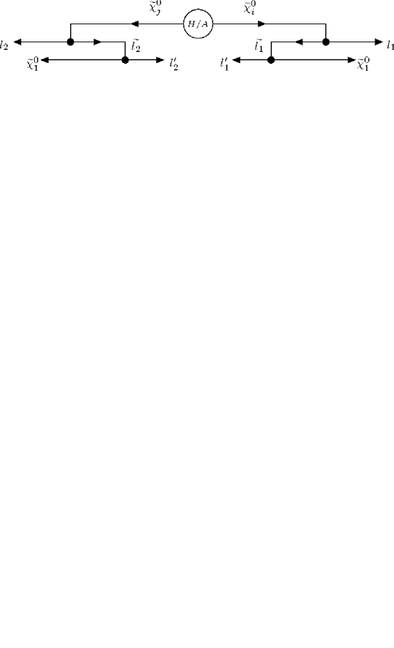
Next, we consider what happens if the two neutralinos in (2) are produced at threshold555This situation was far from realized in  [8], where the Higgs mass was set fairly high, mH400600GeVsimilar-tosubscript𝑚𝐻400600GeVm_{H}\sim 400-600~{}\hbox{GeV}., that is when mH=mi+mjsubscript𝑚𝐻subscript𝑚𝑖subscript𝑚𝑗m_{H}=m_{i}+m_{j} exactly. Now, it turns out, five of the invariants defined above (M4lsubscript𝑀4𝑙M_{4l}, M¯2l2lsubscript¯𝑀2𝑙2𝑙\overline{M}_{2l2l}, M¯l2lsubscript¯𝑀𝑙2𝑙\overline{M}_{l2l}, M¯3lsubscript¯𝑀3𝑙\overline{M}_{3l}, and M¯llsubscript¯𝑀𝑙𝑙\overline{M}_{ll}), in addition to Meesubscript𝑀𝑒𝑒M_{ee} and Mμμsubscript𝑀𝜇𝜇M_{\mu\mu}, are simultaneously maximal when the kinematic configuration shown in Fig. 1 is realized.
Refer to caption

Figure 1: Kinematic configuration which simultaneously maximizes M4lsubscript𝑀4𝑙M_{4l}, M¯2l2lsubscript¯𝑀2𝑙2𝑙\overline{M}_{2l2l}, M¯l2lsubscript¯𝑀𝑙2𝑙\overline{M}_{l2l}, M¯3lsubscript¯𝑀3𝑙\overline{M}_{3l}, M¯llsubscript¯𝑀𝑙𝑙\overline{M}_{ll}, and (Mee×Mμμ)subscript𝑀𝑒𝑒subscript𝑀𝜇𝜇(M_{ee}\times M_{\mu\mu}) at threshold (mH=mi+mjsubscript𝑚𝐻subscript𝑚𝑖subscript𝑚𝑗m_{H}=m_{i}+m_{j}).

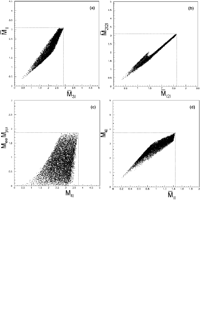
With a suitably large sample of events, we need only plot one invariant against another to get its maximal value, as shown in Figure 2. Note that the endpoints tend to lie at a fairly triangular apex, therefore well-approximated as the intersection of two tangents to the ‘correlation shape’. Moreover, this correlation retains its shape in the presence of backgrounds, since these latter do not have the correct correlations among the various invariants and would tend to form a diffuse halo around the more concentrated signal shape. Compared to the traditional one-dimensional histogram approach, where backgrounds are harder to subtract and endpoints must be fit with a more arbitrary function, the reader can begin to appreciate that a technique using correlated invariants is much more powerful. Though this case of threshold production is not particularly likely in the MSSM, it prepares us for the next step.
Refer to caption
Figure 2: Various correlations of four-lepton invariant masses at threshold (mH=mi+mjsubscript𝑚𝐻subscript𝑚𝑖subscript𝑚𝑗m_{H}=m_{i}+m_{j}). This simulation is purely from relativistic kinematics with (m1,mi,mj,ms)=(1,3,4,1.1)subscript𝑚1subscript𝑚𝑖subscript𝑚𝑗subscript𝑚𝑠1341.1(m_{1},~{}m_{i},~{}m_{j},~{}m_{s})~{}=~{}(1,~{}3,~{}4,~{}1.1) (units arbitrary). Dashed lines mark the maximum value of each invariant.

2.3 Continuous Superposition of Higgses

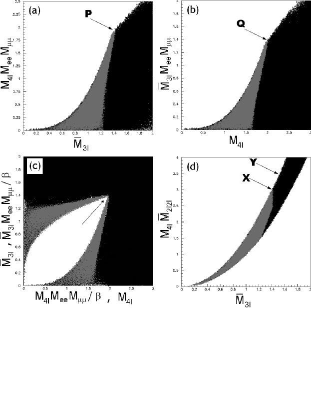
Consider now the case where not a single Higgs decays in (2), but rather a continuum of Higgs with masses in the range mi+mjmH<subscript𝑚𝑖subscript𝑚𝑗subscript𝑚𝐻m_{i}+m_{j}\leq m_{H}<\infty. Fig. 3 shows what to expect for several strategically-chosen666For the specific decay topology (1), it turns out that only certain correlations between invariants are easily analyzed, these being M4lvs.M¯3lMeeMμμformulae-sequencesubscript𝑀4𝑙𝑣𝑠subscript¯𝑀3𝑙subscript𝑀𝑒𝑒subscript𝑀𝜇𝜇M_{4l}~{}vs.~{}\overline{M}_{3l}M_{ee}M_{\mu\mu}, M¯3lvs.M4lMeeMμμformulae-sequencesubscript¯𝑀3𝑙𝑣𝑠subscript𝑀4𝑙subscript𝑀𝑒𝑒subscript𝑀𝜇𝜇\overline{M}_{3l}~{}vs.~{}{M}_{4l}M_{ee}M_{\mu\mu}, M¯3lvs.M4lM¯2l2lformulae-sequencesubscript¯𝑀3𝑙𝑣𝑠subscript𝑀4𝑙subscript¯𝑀2𝑙2𝑙\overline{M}_{3l}~{}vs.~{}{M}_{4l}\overline{M}_{2l2l}, M¯3lvs.M4lM¯l2lformulae-sequencesubscript¯𝑀3𝑙𝑣𝑠subscript𝑀4𝑙subscript¯𝑀𝑙2𝑙\overline{M}_{3l}~{}vs.~{}{M}_{4l}\overline{M}_{l2l}, and M¯llvs.M¯2l2lM¯l2lformulae-sequencesubscript¯𝑀𝑙𝑙𝑣𝑠subscript¯𝑀2𝑙2𝑙subscript¯𝑀𝑙2𝑙\overline{M}_{ll}~{}vs.~{}\overline{M}_{2l2l}\overline{M}_{l2l}. choices of invariants: threshold decays are plotted in gray, while all above-threshold decays are plotted in black777Threshold decays obviously contribute only infinitesimally to the total shape, but for the sake of seeing how these are distributed compared to above-threshold decays, we plotted 103superscript10310^{3} of these on top of 106superscript10610^{6} above-threshold events.. The key observation to make here is that the threshold points P(Q) in Fig. 3a(b) are not at all obscured when above-threshold events are superimposed; in fact, these latter serve to graphically reinforce the threshold points, located on the envelope of the collective shape.

It should be clear, however, that without our color-coding in Fig. 3(a,b), it is not possible to tell the exact position of P and Q888There is a sort of kink near P and Q, but this turns out to be related to M+maxsuperscriptsubscript𝑀superscriptsuperscript𝑚𝑎𝑥M_{\ell^{+}\ell^{-}}^{max} only.. Nevertheless, P and Q share a tight relationship: namely, they must uniquely identify the three endpoints M4lmaxsuperscriptsubscript𝑀4𝑙𝑚𝑎𝑥M_{4l}^{max}, M¯3lmaxsuperscriptsubscript¯𝑀3𝑙𝑚𝑎𝑥\overline{M}_{3l}^{max}, and (Meemax)×(Mμμmax)superscriptsubscript𝑀𝑒𝑒𝑚𝑎𝑥superscriptsubscript𝑀𝜇𝜇𝑚𝑎𝑥(M_{ee}^{max})\times(M_{\mu\mu}^{max}), this last of which is obtainable from a wedgebox plot [10], i.e. a plot of Meevs.Mμμformulae-sequencesubscript𝑀𝑒𝑒𝑣𝑠subscript𝑀𝜇𝜇M_{ee}~{}vs.~{}M_{\mu\mu}. We can therefore find the precise locations of P and Q with a graphical device: superimpose a plot of M4lvs.M¯3l(Mee)×(Mμμ)(Meemax)×(Mμμmax)formulae-sequencesubscript𝑀4𝑙𝑣𝑠subscript¯𝑀3𝑙subscript𝑀𝑒𝑒subscript𝑀𝜇𝜇superscriptsubscript𝑀𝑒𝑒𝑚𝑎𝑥superscriptsubscript𝑀𝜇𝜇𝑚𝑎𝑥M_{4l}~{}vs.~{}\overline{M}_{3l}\frac{(M_{ee})\times(M_{\mu\mu})}{(M_{ee}^{max})\times(M_{\mu\mu}^{max})} with one of M4l(Mee)×(Mμμ)(Meemax)×(Mμμmax)vs.M¯3lformulae-sequencesubscript𝑀4𝑙subscript𝑀𝑒𝑒subscript𝑀𝜇𝜇superscriptsubscript𝑀𝑒𝑒𝑚𝑎𝑥superscriptsubscript𝑀𝜇𝜇𝑚𝑎𝑥𝑣𝑠subscript¯𝑀3𝑙M_{4l}\frac{(M_{ee})\times(M_{\mu\mu})}{(M_{ee}^{max})\times(M_{\mu\mu}^{max})}~{}vs.~{}\overline{M}_{3l} (i.e. superimpose Fig. 3a and Fig. 3b with swapped and rescaled axes). This gives rise to a characteristic ’cat-eye’ shape(Figure 3c), where the upper corner of the eye pinpoints the correct threshold extrema of M4lsubscript𝑀4𝑙M_{4l} and M¯3lsubscript¯𝑀3𝑙\overline{M}_{3l}.

There is another very useful correlation here, namely M¯3lvs.M4lM¯2l2lformulae-sequencesubscript¯𝑀3𝑙𝑣𝑠subscript𝑀4𝑙subscript¯𝑀2𝑙2𝑙\overline{M}_{3l}~{}vs.~{}{M}_{4l}\overline{M}_{2l2l} (see previous footnote for alternatives). Analogous to the situation in Fig. 3a and Fig. 3b, threshold values of M¯3lmaxsuperscriptsubscript¯𝑀3𝑙𝑚𝑎𝑥\overline{M}_{3l}^{max} and M4lmaxM¯2l2lmaxsuperscriptsubscript𝑀4𝑙𝑚𝑎𝑥superscriptsubscript¯𝑀2𝑙2𝑙𝑚𝑎𝑥M_{4l}^{max}\overline{M}_{2l2l}^{max} for this 𝕏χ~i0χ~j0𝕏superscriptsubscript~𝜒𝑖0superscriptsubscript~𝜒𝑗0\mathbb{X}\to{\widetilde{\chi}_{i}}^{0}{\widetilde{\chi}_{j}}^{0} decay again lie on the envelope of the correlation shape at point ‘X’ in Fig. 3d; what is more interesting, every point on the envelope above X (say, ‘Y’ in Fig. 3d) corresponds to another set of M¯3lmaxsuperscriptsubscript¯𝑀3𝑙𝑚𝑎superscript𝑥\overline{M}_{3l}^{max^{\prime}} and M4lmaxM¯2l2lmaxsuperscriptsubscript𝑀4𝑙𝑚𝑎superscript𝑥superscriptsubscript¯𝑀2𝑙2𝑙𝑚𝑎superscript𝑥M_{4l}^{max^{\prime}}\overline{M}_{2l2l}^{max^{\prime}} for a decay 𝕏ζξ𝕏𝜁𝜉\mathbb{X}\to\zeta\xi, where ζ𝜁\zeta and ξ𝜉\xi are some hypothetical set of heavier particles (mζ,ξ>mi,jsubscript𝑚𝜁𝜉subscript𝑚𝑖𝑗m_{\zeta,\xi}>m_{i,j}) which follow the same decay chain through an on-shell slepton to leptons and the LSP. In other words, if ζ𝜁\zeta and ξ𝜉\xi really were produced, they would have decay kinematics leading precisely to the endpoints identified at Y (we will call this a ‘pseudo-threshold’). Every such pseudo-threshold therefore yields a set of endpoints M¯3lmaxsuperscriptsubscript¯𝑀3𝑙𝑚𝑎superscript𝑥\overline{M}_{3l}^{max^{\prime}} and M4lmaxM¯2l2lmaxsuperscriptsubscript𝑀4𝑙𝑚𝑎superscript𝑥superscriptsubscript¯𝑀2𝑙2𝑙𝑚𝑎superscript𝑥M_{4l}^{max^{\prime}}\overline{M}_{2l2l}^{max^{\prime}} which can be used to constrain m1subscript𝑚1m_{1}, mssubscript𝑚𝑠m_{s}, and mζsubscript𝑚𝜁m_{\zeta} (where without loss of generality we can take ζ=ξ𝜁𝜉\zeta=\xi), this latter being merely an auxiliary parameter at each such point. What we are effectively saying here is that the shape of the envelope above X depends on m1subscript𝑚1m_{1} and mssubscript𝑚𝑠m_{s} only, and sufficiently precise measurement of this envelope can constrain these parameters.
Refer to caption
Figure 3: Correlations of various invariant masses in a superposition of many Higgs decays (2) with a continuum of masses in the range mi+mjmH<subscript𝑚𝑖subscript𝑚𝑗subscript𝑚𝐻m_{i}+m_{j}\leq m_{H}<\infty (again from relativistic kinematics only, with (m1,mi=mj,ms)=(1,2,1.5)(m_{1},~{}m_{i}=m_{j},~{}m_{s})~{}=~{}(1,~{}2,~{}1.5) in arbitrary units). Points P and Q in (a) and (b) identify threshold endpoints; these can be found precisely with a ‘cat-eye’ plot in (c), where we have abbreviated β(Meemax)×(Mμμmax)𝛽superscriptsubscript𝑀𝑒𝑒𝑚𝑎𝑥superscriptsubscript𝑀𝜇𝜇𝑚𝑎𝑥\beta\equiv(M_{ee}^{max})\times(M_{\mu\mu}^{max}). In (d) we show another useful correlation of invariants which not only gives threshold endpoints at X, but also ‘pseudo-threshold’ endpoints at any point Y higher up on the envelope.

Now there is really no difference between this situation with a continuously-massed Higgs and that of the decay (1), or more specifically

𝕏𝕏+χ~i0(e~±ee+eχ~10)χ~j0(μ~±μμ+μχ~10)\mathbb{X}\to\mathbb{X}^{\prime}+\widetilde{\chi}_{i}^{0}(\to\tilde{e}^{\pm}{e}^{\mp}\to e^{+}e^{-}\widetilde{\chi}_{1}^{0})~{}\widetilde{\chi}_{j}^{0}(\to\tilde{\mu}^{\pm}{\mu}^{\mp}\to\mu^{+}\mu^{-}\widetilde{\chi}_{1}^{0}) (10)

where 𝕏𝕏\mathbb{X} could be pp𝑝𝑝pp, q~q~~𝑞~superscript𝑞\tilde{q}\tilde{q^{\prime}}, q~g~~𝑞~𝑔\tilde{q}\tilde{g} , g~g~~𝑔~𝑔\tilde{g}\tilde{g}, χ~2±χ~2superscriptsubscript~𝜒2plus-or-minussuperscriptsubscript~𝜒2minus-or-plus\widetilde{\chi}_{2}^{\pm}\widetilde{\chi}_{2}^{\mp} etc., or any two999The present work assumes R-parity is exact, though the general technique does not require this. SUSY particles with a continuous center of mass energy greater than or equal to mi+mjsubscript𝑚𝑖subscript𝑚𝑗m_{i}+m_{j}, while 𝕏superscript𝕏\mathbb{X}^{\prime} are any collection of particles, e.g. hadronic jets, that do not confuse the 4-lepton signal. As long as the neutralino-pair subchains are intact, the mother chain is irrelevant. Note also we do not require the lightest neutralino to be stable, as long as its decay products do not include leptons. As we shall see in the next section this technique works very well in MC simulations with a minimal requirement of four isolated leptons plus missing energy.

3 Examples of Applications

In this section we demonstrate the robustness of our technique at two different MSSM parameter points with varying decay topologies. Our MC setup uses HERWIG 6.5 and private codes as in our previous publications  [8, 9, 10] and the reader is referred to these for details.

We generate events

pp{q~,g~,χ~1,2±,χ~1,2,3,40}+{q~,g~,χ~1,2±,χ~1,2,3,40}𝑝𝑝~𝑞~𝑔superscriptsubscript~𝜒12plus-or-minussuperscriptsubscript~𝜒12340~𝑞~𝑔superscriptsubscript~𝜒12plus-or-minussuperscriptsubscript~𝜒12340pp\to\{\tilde{q},\tilde{g},\widetilde{\chi}_{1,2}^{\pm},\widetilde{\chi}_{1,2,3,4}^{0}\}+\{\tilde{q},\tilde{g},\widetilde{\chi}_{1,2}^{\pm},\widetilde{\chi}_{1,2,3,4}^{0}\} (11)

for 1030fb11030𝑓superscript𝑏110-30~{}fb^{-1}(a low-luminosity year at the LHC) and only pass those which decay to a hard and isolated e+esuperscript𝑒superscript𝑒e^{+}e^{-} and μ+μsuperscript𝜇superscript𝜇\mu^{+}\mu^{-} pair with sufficient missing energy( / ET>20GeV / subscript𝐸𝑇20GeV\hbox to0.0pt{\hbox to12.00859pt{\hfil/\hfil}\hss}E_{T}~{}>~{}20\,\hbox{GeV}). This eliminates SM backgrounds aside from ppZZ𝑝𝑝superscript𝑍𝑍pp\to Z^{*}Z, though this can be modeled and subtracted (by a Z-veto if necessary, which happens to work perfectly at the parameter points we will consider). SUSY backgrounds fall into two categories: those which produce exactly four leptons and those which produce more than this (presumably losing some to isolation cuts, detector effects, etc.). The first category includes slepton or chargino ‘3+1’ decays such as χ~2±(l±l±lννν¯χ~10)χ~1(l′′ν′′χ~10)\widetilde{\chi}_{2}^{\pm}(\to{l}^{\pm}{l^{\prime}}^{\pm}{l^{\prime}}^{\mp}~{}\nu\nu^{\prime}\overline{\nu^{\prime}}~{}\widetilde{\chi}_{1}^{0})~{}\widetilde{\chi}_{1}^{\mp}(\to{l^{\prime\prime}}^{\mp}~{}\nu^{\prime\prime}~{}\widetilde{\chi}_{1}^{0}) where one decay goes to three leptons and the other to one. These could always be substantially reduced via flavor subtraction, but this is not necessary since they have totally different kinematics from a ‘2+2’ decay (i.e. (10)) and should not obscure the envelopes in plots such as Fig. 3. Moreover, such decays would exhibit their own characteristic correlation shapes in addition to the trilepton invariant mass edge. In the worst case, then, four-lepton SUSY backgrounds should be considered an ‘enriched signal.’ The second category of SUSY backgrounds includes events such as τ~τ~~𝜏~𝜏\tilde{\tau}\tilde{\tau} where each stau decays τ~τχ~20l±l±lννχ~10~𝜏𝜏superscriptsubscript~𝜒20superscript𝑙plus-or-minussuperscriptsuperscript𝑙plus-or-minussuperscriptsuperscript𝑙minus-or-plus𝜈superscript𝜈superscriptsubscript~𝜒10\tilde{\tau}\to\tau\widetilde{\chi}_{2}^{0}\to{l}^{\pm}{l^{\prime}}^{\pm}{l^{\prime}}^{\mp}~{}\nu\nu^{\prime}\widetilde{\chi}_{1}^{0} and two of the total of six leptons are somehow lost. Yet such events, if not made utterly small by leptonic branching fractions, would introduce a more-or-less diffuse halo in our correlation plots, and in particular should not confuse the identification of threshold points.

3.1 On-Shell Box

The most basic illustration of the HT technique for the decay (10) is when only one particular (i,j)𝑖𝑗(i,j)-combination has a significant branching ratio; if, in addition, i=j𝑖𝑗i=j, threshold endpoint formulae simplify dramatically, e.g.

M4lmax=mj2(2mj2ms2m12)ms4mjms2superscriptsubscript𝑀4𝑙𝑚𝑎𝑥superscriptsubscript𝑚𝑗22superscriptsubscript𝑚𝑗2superscriptsubscript𝑚𝑠2superscriptsubscript𝑚12superscriptsubscript𝑚𝑠4subscript𝑚𝑗superscriptsubscript𝑚𝑠2{M}_{4l}^{max}=\frac{m_{j}^{2}(2m_{j}^{2}m_{s}^{2}-m_{1}^{2})-m_{s}^{4}}{m_{j}m_{s}^{2}} (12)

A χ~20χ~20superscriptsubscript~𝜒20superscriptsubscript~𝜒20\widetilde{\chi}_{2}^{0}\widetilde{\chi}_{2}^{0} pair, for example, is often the chief product of colored cascades at mSUGRA points such as SPS1a [3]. Though we have checked our technique works at SPS1a, we choose another point which has higher rates and therefore better demonstrates the agreement with theory presented in the last section:

On-Shell Point
μ=250GeVM2=250GeVM1=125GeVformulae-sequence𝜇250GeVformulae-sequencesubscript𝑀2250GeVsubscript𝑀1125GeV\displaystyle\mu=250\,\hbox{GeV}~{}~{}~{}~{}~{}~{}M_{2}=250\,\hbox{GeV}~{}~{}~{}~{}~{}~{}M_{1}=125\,\hbox{GeV}
tanβ=10Mτ~,(e~,μ~)L=250GeVM(e~,μ~)R=130GeVformulae-sequence𝛽10formulae-sequencesubscript𝑀~𝜏subscript~𝑒~𝜇𝐿250GeVsubscript𝑀subscript~𝑒~𝜇𝑅130GeV\displaystyle\tan\beta=10~{}~{}~{}~{}~{}~{}M_{\tilde{\tau},(\tilde{e},\tilde{\mu})_{L}}=250\,\hbox{GeV}~{}~{}~{}~{}~{}~{}M_{(\tilde{e},\tilde{\mu})_{R}}=130\,\hbox{GeV}
mH=700GeVMq~400GeVMg~500GeVformulae-sequencesubscript𝑚𝐻700GeVformulae-sequencesubscript𝑀~𝑞400GeVsubscript𝑀~𝑔500GeV\displaystyle m_{H}=700\,\hbox{GeV}~{}~{}~{}~{}M_{\tilde{q}}\approx 400\,\hbox{GeV}~{}~{}~{}~{}M_{\tilde{g}}\approx 500\,\hbox{GeV}

Here we have raised the left-handed slepton and stau soft mass inputs above those of the right-handed selectron and smuon (note the physical masses differ slightly from these, see Table 1) to suppress sneutrino exchange and stau modes which may reduce the magnitude of (but not character of) the signal. The heavy Higgs mass is set rather high to remove it from the analysis, but setting it lower would in fact be beneficial since Higgs contribute to the signal process 𝕏χ~i0χ~j0𝕏superscriptsubscript~𝜒𝑖0superscriptsubscript~𝜒𝑗0\mathbb{X}\to\widetilde{\chi}_{i}^{0}\widetilde{\chi}_{j}^{0}.

Table 1: Relevant masses at the On-Shell Point and Off-Shell Point (all masses in GeV).
χ~10subscriptsuperscript~𝜒01{\widetilde{\chi}}^{0}_{1} χ~20subscriptsuperscript~𝜒02{\widetilde{\chi}}^{0}_{2} χ~30subscriptsuperscript~𝜒03{\widetilde{\chi}}^{0}_{3} χ~40subscriptsuperscript~𝜒04{\widetilde{\chi}}^{0}_{4} e~R,μ~Rsubscript~𝑒𝑅subscript~𝜇𝑅\tilde{e}_{R},\tilde{\mu}_{R} χ~1±subscriptsuperscript~𝜒plus-or-minus1{\widetilde{\chi}}^{\pm}_{1} χ~2±subscriptsuperscript~𝜒plus-or-minus2{\widetilde{\chi}}^{\pm}_{2}
On-Shell 117.1117.1117.1 197.5197.5197.5 257.2257.2257.2 317.7317.7317.7 134.7134.7134.7 193.3193.3193.3 317.0317.0317.0
Off-Shell 79.679.679.6 131.5131.5131.5 160.6160.6160.6 249.5249.5249.5 148.0148.0148.0 115.6115.6115.6 249.0249.0249.0

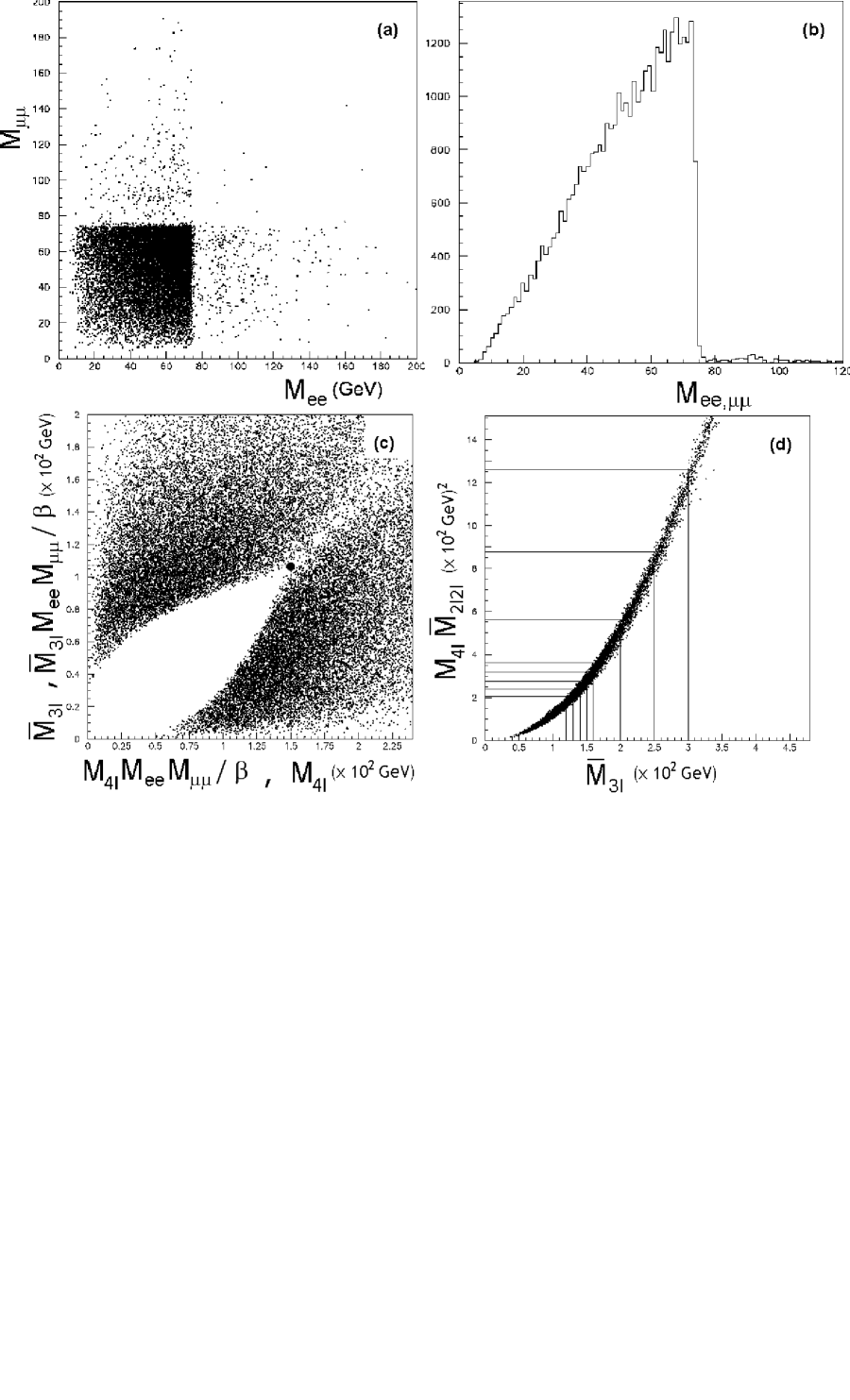
With a luminosity of 30fb130𝑓superscript𝑏130~{}fb^{-1} the wedgebox plot in Figure 4a is a very dense and symmetric box structure, which strongly suggests degenerate neutralinos decaying via degenerate sleptons101010Strictly speaking this could also be a chargino decaying via a sneutrino, i.e. χ~2±l±ν~l±lχ~1±superscriptsubscript~𝜒2plus-or-minussuperscript𝑙plus-or-minus~𝜈superscript𝑙plus-or-minussuperscript𝑙minus-or-plussuperscriptsubscript~𝜒1plus-or-minus\widetilde{\chi}_{2}^{\pm}\to l^{\pm}\tilde{\nu}\to l^{\pm}l^{\mp}\widetilde{\chi}_{1}^{\pm}. Other signs such as the number of 6-lepton events(after χ~1±l±νχ~10superscriptsubscript~𝜒1plus-or-minussuperscript𝑙plus-or-minus𝜈superscriptsubscript~𝜒10\widetilde{\chi}_{1}^{\pm}\to l^{\pm}\nu\widetilde{\chi}_{1}^{0}) might resolve this ambiguity.. Since the dilepton mass distribution(Figure 4b) is quite triangular, we could also guess that the sleptons are on-shell — in the next subsection we will show how to establish this quantitatively.
Refer to caption
Figure 4: Various plots for the On-Shell Point with 30fb130𝑓superscript𝑏130~{}fb^{-1} luminosity. The wedgebox plot (a) is mostly box-like with a triangular dilepton mass distribution (b) typifying an on-shell decay. The threshold values of M4lsubscript𝑀4𝑙M_{4l} and M¯3lsubscript¯𝑀3𝑙\overline{M}_{3l} for the χ~20χ~20superscriptsubscript~𝜒20superscriptsubscript~𝜒20\widetilde{\chi}_{2}^{0}\widetilde{\chi}_{2}^{0} resonance (β=(75GeV)2𝛽superscript75GeV2\beta=(75\,\hbox{GeV})^{2}) in the cat-eye plot (c) are easily identified at the ‘corner of the eye’ (the black dot). We proceed to measure several points along the envelope of the shape in (d) for M¯3l>M¯3lmaxsubscript¯𝑀3𝑙superscriptsubscript¯𝑀3𝑙𝑚𝑎𝑥\overline{M}_{3l}>\overline{M}_{3l}^{max}; these can be used to constrain the slepton and LSP masses.

Thus, being certain of having a fairly homogenous sample of 𝕏χ~20χ~20𝕏superscriptsubscript~𝜒20superscriptsubscript~𝜒20\mathbb{X}\to\widetilde{\chi}_{2}^{0}\widetilde{\chi}_{2}^{0} decays, where each neutralino decays as χ~20~±+χ~20superscriptsubscript~𝜒20superscript~plus-or-minussuperscriptminus-or-plussuperscriptsuperscriptsuperscriptsubscript~𝜒20\widetilde{\chi}_{2}^{0}\to\tilde{\ell}^{\pm}{\ell}^{\mp}\to\ell^{+}\ell^{-}\widetilde{\chi}_{2}^{0} with a dilepton edge M+75GeVsimilar-tosubscript𝑀superscriptsuperscript75GeVM_{\ell^{+}\ell^{-}}\sim~{}75\,\hbox{GeV}, we can directly proceed to construct a cat-eye plot in Fig. 4c to determine threshold values of M4lmaxsuperscriptsubscript𝑀4𝑙𝑚𝑎𝑥{M}_{4l}^{max} and M¯3lmaxsuperscriptsubscript¯𝑀3𝑙𝑚𝑎𝑥\overline{M}_{3l}^{max}. Note that even at this low luminosity, the threshold point (marked as a large black dot in Fig. 4c) can be located to a few GeV precision: we measure (M4lmax,M¯3lmax)=(150±5,107±5)GeVsuperscriptsubscript𝑀4𝑙𝑚𝑎𝑥superscriptsubscript¯𝑀3𝑙𝑚𝑎𝑥plus-or-minus1505plus-or-minus1075GeV({M}_{4l}^{max},\overline{M}_{3l}^{max})=(150\pm 5,107\pm 5)\,\hbox{GeV}. This is quite close to the expected values of (153.9,112.4)GeV153.9112.4GeV(153.9,112.4)\,\hbox{GeV} found by plugging in masses from Table 1 into formulae in the Appendix. The HT method is working.

Having determined M¯3lmaxsuperscriptsubscript¯𝑀3𝑙𝑚𝑎𝑥\overline{M}_{3l}^{max} from the cat-eye plot, we proceed to measure a number of pseudo-threshold points in a plot of M¯3lvs.M4lM¯2l2lformulae-sequencesubscript¯𝑀3𝑙𝑣𝑠subscript𝑀4𝑙subscript¯𝑀2𝑙2𝑙\overline{M}_{3l}~{}vs.~{}{M}_{4l}\overline{M}_{2l2l} for M¯3l>M¯3lmaxsubscript¯𝑀3𝑙superscriptsubscript¯𝑀3𝑙𝑚𝑎𝑥\overline{M}_{3l}>\overline{M}_{3l}^{max} (see Fig. 4d). Table 2 compares some of our measurements to expected values over a liberal range of M¯3lsubscript¯𝑀3𝑙\overline{M}_{3l}, where the reader can verify good agreement. Using a large number n𝑛n of measurements (say n=30𝑛30n=30) we search (m1,ms,mζ1,mζ2,mζn)subscript𝑚1subscript𝑚𝑠subscript𝑚subscript𝜁1subscript𝑚subscript𝜁2subscript𝑚subscript𝜁𝑛(m_{1},m_{s},m_{\zeta_{1}},m_{\zeta_{2}},...m_{\zeta_{n}})-space for the best fit to the corresponding (M¯3lmax,M4lmaxM¯2l2lmax)i=1..n(\overline{M}_{3l}^{max},{M}_{4l}^{max}\overline{M}_{2l2l}^{max})_{i=1..n}, using analytical expressions in the Appendix. We find m1=116±10GeVsubscript𝑚1plus-or-minus11610GeVm_{1}=116\pm 10\,\hbox{GeV} with the slepton mass shifted by a near constant, ms=(m1+17)±2GeVsubscript𝑚𝑠plus-or-minussubscript𝑚1172GeVm_{s}=(m_{1}+17)\pm 2\,\hbox{GeV}. From these and the dilepton edge M+=75±1GeVsubscript𝑀superscriptsuperscriptplus-or-minus751GeVM_{\ell^{+}\ell^{-}}=~{}75\pm 1\,\hbox{GeV}, we can likewise determine m2=210±12GeVsubscript𝑚2plus-or-minus21012GeVm_{2}=210\pm 12\,\hbox{GeV}. With a higher luminosity sample (say, 300fb1300𝑓superscript𝑏1300~{}fb^{-1}) error-bars could certainly be reduced by a factor of several; in this case the masses (m1,ms,m2)subscript𝑚1subscript𝑚𝑠subscript𝑚2(m_{1},m_{s},m_{2}) can ultimately be found to about 2% accuracy.

Table 2: Measurements of M4lM¯2l2lsubscript𝑀4𝑙subscript¯𝑀2𝑙2𝑙{M}_{4l}\overline{M}_{2l2l} for various M¯3lsubscript¯𝑀3𝑙\overline{M}_{3l} at the On-Shell Point (viz. Fig. 4d) and comparison to theoretical values (boldface) assuming these correspond to pseudo-thresholds, i.e. plugging slepton and LSP masses from Table 1 and mζsubscript𝑚𝜁m_{\zeta} (in place of mjsubscript𝑚𝑗m_{j}) into formulae in the Appendix (all masses in GeV).
M¯3lsubscript¯𝑀3𝑙\overline{M}_{3l} M4lM¯2l2lsubscript𝑀4𝑙subscript¯𝑀2𝑙2𝑙{M}_{4l}\overline{M}_{2l2l} Theory mζsubscript𝑚𝜁m_{\zeta}
120 205±1plus-or-minus2051205\pm 1 205.6 203.2
130 239±1plus-or-minus2391239\pm 1 240.3 211.0
140 275±2plus-or-minus2752275\pm 2 278.0 219.0
150 318±2plus-or-minus3182318\pm 2 318.0 227.0
160 363±2plus-or-minus3632363\pm 2 360.9 235.2
200 560±5plus-or-minus5605560\pm 5 559.9 269.0
250 875±5plus-or-minus8755875\pm 5 868.0 313.0
300 1260±5plus-or-minus126051260\pm 5 1250.6 595.5

3.2 Off-Shell Box

Decays through off-shell sleptons are simpler for two reasons. First, mathematically speaking, invariant mass edges do not depend on slepton masses; in the case of a box topology these can therefore only depend on m1subscript𝑚1m_{1} and mjsubscript𝑚𝑗m_{j}. Since the dilepton mass edge is equal to the difference of these, (mjm1)subscript𝑚𝑗subscript𝑚1(m_{j}-m_{1}), we only need one other function of these masses to determine them.

Secondly, the physical degrees of freedom are easier to analyze: for threshold decays in particular, each neutralino χ~j0superscriptsubscript~𝜒𝑗0\widetilde{\chi}_{j}^{0} is at rest in the center of mass frame and leptonic invariants are maximized/minimized when the same flavor leptons are emitted antiparallel/parallel. The product (Mee)×(Mμμ)subscript𝑀𝑒𝑒subscript𝑀𝜇𝜇(M_{ee})\times(M_{\mu\mu}) is therefore maximal when the electron(muon) is antiparallel to the positron(anti-muon), and is equal to (mjm1)2superscriptsubscript𝑚𝑗subscript𝑚12(m_{j}-m_{1})^{2}. For this kinematical configuration, however, all the other invariants M4lsubscript𝑀4𝑙M_{4l}, M¯2l2lsubscript¯𝑀2𝑙2𝑙\overline{M}_{2l2l}, M¯l2lsubscript¯𝑀𝑙2𝑙\overline{M}_{l2l}, M¯3lsubscript¯𝑀3𝑙\overline{M}_{3l}, and M¯llsubscript¯𝑀𝑙𝑙\overline{M}_{ll} are equal(up to a constant factor) to (mjm1)subscript𝑚𝑗subscript𝑚1(m_{j}-m_{1}) and therefore do not provide independent information.

The trick is to consider configurations where the electron and positron are antiparallel while the muon and anti-muon are parallel (or vice versa). In this case Meesubscript𝑀𝑒𝑒M_{ee} or Mμμsubscript𝑀𝜇𝜇M_{\mu\mu} is maximal and the other invariants (excepting M¯l2lsubscript¯𝑀𝑙2𝑙\overline{M}_{l2l}) unconditionally attain minima when the e+esuperscript𝑒superscript𝑒e^{+}e^{-} pair is emitted at right angles to the μ+μsuperscript𝜇superscript𝜇\mu^{+}\mu^{-} pair:

M¯4l,2l2l,3l,llminsuperscriptsubscript¯𝑀4𝑙2𝑙2𝑙3𝑙𝑙𝑙𝑚𝑖𝑛\displaystyle\overline{M}_{4l,2l2l,3l,ll}^{min} =\displaystyle= (mjm1)(α+βm1mj+γm12mj2ξ)14subscript𝑚𝑗subscript𝑚1superscript𝛼𝛽subscript𝑚1subscript𝑚𝑗𝛾superscriptsubscript𝑚12superscriptsubscript𝑚𝑗2𝜉14\displaystyle(m_{j}-m_{1})\left(\frac{\alpha+\beta\frac{m_{1}}{m_{j}}+\gamma\frac{m_{1}^{2}}{m_{j}^{2}}}{\xi}\right)^{\frac{1}{4}} (13)

for specific values of the parameters α𝛼\alpha, β𝛽\beta, γ𝛾\gamma, and ξ𝜉\xi listed in Table 3. Thus, any one of these in conjunction with the dilepton mass edge uniquely determines mjsubscript𝑚𝑗m_{j} and m1subscript𝑚1m_{1}. Geometrically, these endpoints are found at the intersection of the line Ml+l=(mjm1)subscript𝑀superscript𝑙superscript𝑙subscript𝑚𝑗subscript𝑚1M_{l^{+}l^{-}}=(m_{j}-m_{1}) with the near edges of the correlation shapes on a plot of Ml+lsubscript𝑀superscript𝑙superscript𝑙M_{l^{+}l^{-}} versus M4lsubscript𝑀4𝑙M_{4l}, M¯2l2lsubscript¯𝑀2𝑙2𝑙\overline{M}_{2l2l}, M¯3lsubscript¯𝑀3𝑙\overline{M}_{3l}, or M¯llsubscript¯𝑀𝑙𝑙\overline{M}_{ll}. These intersections can be found with high precision and then checked against eachother for consistency.

To see the efficacy of this method, consider the following parameter point (see Table 1 again for the physical spectrum):

Off-Shell Point
μ=150GeVM2=200GeVM1=100GeVformulae-sequence𝜇150GeVformulae-sequencesubscript𝑀2200GeVsubscript𝑀1100GeV\displaystyle\mu=150\,\hbox{GeV}~{}~{}~{}~{}M_{2}=200\,\hbox{GeV}~{}~{}~{}~{}M_{1}=100\,\hbox{GeV}
tanβ=10Mτ~,(e~,μ~)L=300GeVM(e~,μ~)R=135GeVformulae-sequence𝛽10formulae-sequencesubscript𝑀~𝜏subscript~𝑒~𝜇𝐿300GeVsubscript𝑀subscript~𝑒~𝜇𝑅135GeV\displaystyle\tan\beta=10~{}~{}~{}~{}M_{\tilde{\tau},(\tilde{e},\tilde{\mu})_{L}}=300\,\hbox{GeV}~{}~{}~{}~{}~{}~{}~{}~{}M_{(\tilde{e},\tilde{\mu})_{R}}=135\,\hbox{GeV}
mH=700GeVMq~300GeVMg~350GeVsubscript𝑚𝐻700GeVsubscript𝑀~𝑞300GeVsubscript𝑀~𝑔350GeV\displaystyle m_{H}=700\,\hbox{GeV}~{}~{}~{}M_{\tilde{q}}\approx 300\,\hbox{GeV}~{}~{}~{}M_{\tilde{g}}\approx 350\,\hbox{GeV}
Refer to caption
Refer to caption
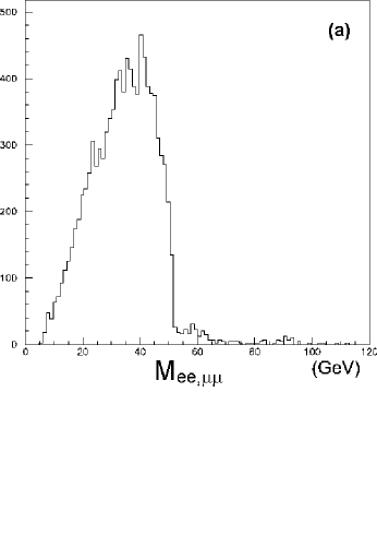
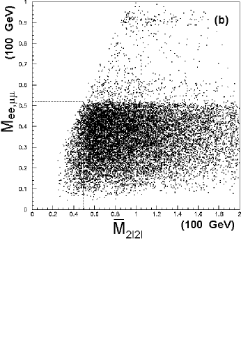
Figure 5: MC Simulation at the Off-Shell Point for 10fb110𝑓superscript𝑏110~{}fb^{-1} luminosity. The dilepton invariant mass distribution in (a) indicates a maximum of about Ml+lmax52GeVsimilar-tosuperscriptsubscript𝑀superscript𝑙superscript𝑙𝑚𝑎𝑥52GeVM_{l^{+}l^{-}}^{max}\sim 52\,\hbox{GeV}. In (b) we show where this maximum is coincident with the minimum value of M¯2l2lsubscript¯𝑀2𝑙2𝑙\overline{M}_{2l2l} at the dotted line, which is to be matched against expression (13). Corresponding plots for the other invariants look very similar.

Though the 10fb110𝑓superscript𝑏110~{}fb^{-1} dilepton mass distribution in Fig. 5a looks very similar to that of the On-Shell Point, the dilepton edge at Ml+lmax52GeVsimilar-tosuperscriptsubscript𝑀superscript𝑙superscript𝑙𝑚𝑎𝑥52GeVM_{l^{+}l^{-}}^{max}\sim 52\,\hbox{GeV} is in fact due to three-body decays via off-shell sleptons. We might guess this from the vaguely less-than-triangular shape, but now we have a better way. We simply plot Ml+lsubscript𝑀superscript𝑙superscript𝑙M_{l^{+}l^{-}} versus each of the invariants M4lsubscript𝑀4𝑙M_{4l}, M¯2l2lsubscript¯𝑀2𝑙2𝑙\overline{M}_{2l2l}, M¯3lsubscript¯𝑀3𝑙\overline{M}_{3l}, and M¯llsubscript¯𝑀𝑙𝑙\overline{M}_{ll} (e.g. Fig. 5(b)) and match against the formulae in (13). Table 3 shows that these give mutually consistent values of m1subscript𝑚1m_{1} and mjsubscript𝑚𝑗m_{j}, which at high luminosity may be determined to several percent or so. Had we constructed the same plots at our On-Shell Point, we would have obtained a set of endpoints which give inconsistent, even nonsensical values for m1,jsubscript𝑚1𝑗m_{1,j} (e.g. negative LSP mass!). Though the dilepton distributions of Fig. 4b and Fig. 5a give qualitative hints of whether sleptons are on- or off-shell, here we seem to have the first definitively quantitative method of determining this which succeeds even with modest(several GeV) endpoint precision.

Table 3: Offshell Decay Parameters in (13) and Fits to MC data at the Off-Shell Point for the LSP mass (m1subscript𝑚1m_{1}), assuming the dilepton edges are exact and 0.2GeV0.2GeV0.2\,\hbox{GeV} precision on other endpoints. Also shown are attempted fits to data at the On-Shell Point which, even with larger(±1GeVplus-or-minus1GeV\pm 1\,\hbox{GeV}) errors, give self-inconsistent results.
Invariant α𝛼\alpha β𝛽\beta γ𝛾\gamma ξ𝜉\xi LSP(Off) LSP(On)
M4lminsuperscriptsubscript𝑀4𝑙𝑚𝑖𝑛M_{4l}^{min} 4 4 1 1 85±5plus-or-minus85585\pm 5 22±5plus-or-minus22522\pm 5
M¯2l2lminsuperscriptsubscript¯𝑀2𝑙2𝑙𝑚𝑖𝑛\overline{M}_{2l2l}^{min} 2 0 1 3 85±11plus-or-minus851185\pm 11 172±78plus-or-minus17278172\pm 78
M¯3lminsuperscriptsubscript¯𝑀3𝑙𝑚𝑖𝑛\overline{M}_{3l}^{min} 11 10 3 8 84±6plus-or-minus84684\pm 6 1±5plus-or-minus151\pm 5
M¯llminsuperscriptsubscript¯𝑀𝑙𝑙𝑚𝑖𝑛\overline{M}_{ll}^{min} 3 2 1 48 86±15plus-or-minus861586\pm 15 8±10plus-or-minus810-8\pm 10

4 Conclusions

Let us now summarize the HT technique and how we applied it in this work:

  1. 1.

    DEFINE the decay chain 𝕏𝕏+ABCnjjets+nlleptons𝕏superscript𝕏𝐴𝐵𝐶subscript𝑛𝑗jetssubscript𝑛lleptons\mathbb{X}\to\mathbb{X^{\prime}}+ABC...\to n_{j}~{}\mathrm{jets}+n_{\textit{l}}~{}\mathrm{leptons}, where 𝕏𝕏\mathbb{X} is anything and 𝕏superscript𝕏\mathbb{X^{\prime}} is exclusive of jets and leptons. In our case this was 𝕏χ~i0χ~j0𝕏superscriptsubscript~𝜒𝑖0superscriptsubscript~𝜒𝑗0\mathbb{X}\to\widetilde{\chi}_{i}^{0}\widetilde{\chi}_{j}^{0} where each neutralino then decayed via a slepton to a pair of leptons and the LSP.

  2. 2.

    DERIVE analytic expressions for all jet and lepton invariant mass endpoints as functions of NP masses, and find kinematic configurations for which two or more of these are extremal at threshold production. In our case of four leptons(nl=4subscript𝑛𝑙4n_{l}=4 ), there are in principle 7 independent invariants; of these, we found (Mee)×(Mμμ)subscript𝑀𝑒𝑒subscript𝑀𝜇𝜇(M_{ee})\times(M_{\mu\mu}), M4lsubscript𝑀4𝑙M_{4l}, M¯2l2lsubscript¯𝑀2𝑙2𝑙\overline{M}_{2l2l}, M¯l2lsubscript¯𝑀𝑙2𝑙\overline{M}_{l2l}, M¯3lsubscript¯𝑀3𝑙\overline{M}_{3l}, and M¯llsubscript¯𝑀𝑙𝑙\overline{M}_{ll} were simultaneously maximal for on-shell decays, wheareas for off-shell decays Meesubscript𝑀𝑒𝑒M_{ee}(Mμμ)M_{\mu\mu}) was maximal(minimal) where M4lsubscript𝑀4𝑙M_{4l}, M¯2l2lsubscript¯𝑀2𝑙2𝑙\overline{M}_{2l2l}, M¯3lsubscript¯𝑀3𝑙\overline{M}_{3l}, and M¯llsubscript¯𝑀𝑙𝑙\overline{M}_{ll} were minimal.

  3. 3.

    DISPLAY correlations of the above invariants in a scatterplot which makes their threshold endpoints visually obvious. Use these to solve for NP masses. For off-shell slepton decays it sufficed to plot each invariant versus Ml+lsubscript𝑀superscript𝑙superscript𝑙M_{l^{+}l^{-}} and note the intersection with the line Ml+l=Ml+lmaxsubscript𝑀superscript𝑙superscript𝑙superscriptsubscript𝑀superscript𝑙superscript𝑙𝑚𝑎𝑥M_{l^{+}l^{-}}=M_{l^{+}l^{-}}^{max}. For on-shell decays we found it useful to make a cat-eye plot to find the threshold value of M¯3lmaxsuperscriptsubscript¯𝑀3𝑙𝑚𝑎𝑥\overline{M}_{3l}^{max}, followed by measuring several pseudo-thresholds in a plot of M¯3lvs.M4lM¯2l2lformulae-sequencesubscript¯𝑀3𝑙𝑣𝑠subscript𝑀4𝑙subscript¯𝑀2𝑙2𝑙\overline{M}_{3l}~{}vs.~{}M_{4l}\overline{M}_{2l2l}. Matching to analytical expressions constrains (m1,m2,ms)subscript𝑚1subscript𝑚2subscript𝑚𝑠(m_{1},m_{2},m_{s}) to within a few percent of their nominal values.

Let us add a few remarks on these three steps. The first step depends of course on the specific NP model under consideration, but once a decay chain has been selected, deriving analytical formulae for endpoints in the second step is not difficult: the sought-after kinematic configuration is usually where each jet or lepton is emitted at a polar angle of θ=0𝜃0\theta=0 or θ=π𝜃𝜋\theta=\pi or perhaps θ=π/2𝜃𝜋2\theta=\pi/2 (for minima) in the frame of the decaying parent particle, backwards Lorentz-boosting to the center-of-mass frame (see Appendix of  [8] for an example). Choosing which invariants to plot in the third step is a matter of trial-and-error — kinematic simulation (as in Fig. 2 and Fig. 3) can be used to see which correlations have a visible threshold point when above-threshold decays are superimposed.

To demonstrate the general applicability of this technique to NP, we present below a partial spectrum of examples. Each example in itself entails numerous variations(e.g. on-shell intermediate states could likewise be taken off-shell):

  • Neutralino Decay via higgs: χ~20χ~20(χ~10h(bb))annotatedsuperscriptsubscript~𝜒20superscriptsubscript~𝜒20absentannotatedsuperscriptsubscript~𝜒10absent𝑏𝑏\widetilde{\chi}_{2}^{0}\widetilde{\chi}_{2}^{0}(\to\widetilde{\chi}_{1}^{0}h(\to bb)). This nj=4subscript𝑛𝑗4n_{j}=4 decay is a potential competitor to the sleptonic modes considered in this paper.

  • Sneutrino Pair Production: ν~ν~(l±χ~1(χ~10W(lν)))annotated~𝜈~𝜈absentannotatedsuperscript𝑙plus-or-minussuperscriptsubscript~𝜒1minus-or-plusabsentannotatedsuperscriptsubscript~𝜒10superscript𝑊absentsuperscript𝑙minus-or-plussuperscript𝜈\tilde{\nu}\tilde{\nu}(\to l^{\pm}\widetilde{\chi}_{1}^{\mp}(\to\widetilde{\chi}_{1}^{0}W^{-}(\to l^{\prime\mp}\nu^{\prime}))) Here nl=4subscript𝑛𝑙4n_{l}=4 as for neutralino pair production, but with totally different kinematics: one can analogously define M4lsubscript𝑀4𝑙M_{4l}, M¯2l2lsubscript¯𝑀2𝑙2𝑙\overline{M}_{2l2l}, M¯l3lsubscript¯𝑀𝑙3𝑙\overline{M}_{l3l}, etc., though threshold extrema of these will have a different correlation.

  • Chargino Pair Production: χ~2±χ~2(lν~(l±χ~1(lνχ~10)))annotatedsuperscriptsubscript~𝜒2plus-or-minussuperscriptsubscript~𝜒2minus-or-plusabsentannotatedsuperscript𝑙minus-or-plus~𝜈absentannotatedsuperscript𝑙plus-or-minussuperscriptsubscript~𝜒1minus-or-plusabsentsuperscript𝑙minus-or-plus𝜈superscriptsubscript~𝜒10\widetilde{\chi}_{2}^{\pm}\widetilde{\chi}_{2}^{\mp}(\to l^{\mp}\tilde{\nu}(\to l^{\pm}\widetilde{\chi}_{1}^{\mp}(\to l^{\mp}\nu{\widetilde{\chi}_{1}}^{0}))) This is a nl=6subscript𝑛𝑙6n_{l}=6 case which means there are as many as 45 relativistic invariants111111The number of invariants is computed as the number of pairwise contractions among the observable momenta, as well as with powers of ϵμνρσsuperscriptitalic-ϵ𝜇𝜈𝜌𝜎\epsilon^{\mu\nu\rho\sigma}.

  • Slepton Pair Production l~±l~(lχ~20(l±lχ~10))annotatedsuperscript~𝑙plus-or-minussuperscript~𝑙minus-or-plusabsentannotatedsuperscript𝑙minus-or-plussuperscriptsubscript~𝜒20absentsuperscript𝑙plus-or-minussuperscript𝑙minus-or-plussuperscriptsubscript~𝜒10\tilde{l}^{\pm}\tilde{l}^{\mp}(\to l^{\mp}\widetilde{\chi}_{2}^{0}(\to l^{\pm}l^{\mp}\widetilde{\chi}_{1}^{0})). This could either be nl=6subscript𝑛𝑙6n_{l}=6 or nl=4subscript𝑛𝑙4n_{l}=4 depending on how the other slepton decays.

  • Squark Pair Production q~q~(qχ~20(l±l~(lχ~10)))annotated~𝑞~𝑞absentannotated𝑞superscriptsubscript~𝜒20absentannotatedsuperscript𝑙plus-or-minussuperscript~𝑙minus-or-plusabsentsuperscript𝑙minus-or-plussuperscriptsubscript~𝜒10\tilde{q}\tilde{q}(\to q\widetilde{\chi}_{2}^{0}(\to l^{\pm}\tilde{l}^{\mp}(\to l^{\mp}\widetilde{\chi}_{1}^{0}))). A nj=2subscript𝑛𝑗2n_{j}=2, nl=4subscript𝑛𝑙4n_{l}=4 decay with 45 invariants to analyze.

  • Gluino Pair Production g~g~(qq~(qχ~20(qqχ~10))\tilde{g}\tilde{g}(\to q\tilde{q}(\to q\widetilde{\chi}_{2}^{0}(\to q^{\prime}q^{\prime}\widetilde{\chi}_{1}^{0})) This nj=8subscript𝑛𝑗8n_{j}=8 decay has an astounding 588588588 invariants.

  • Nonstandard Higgs decays hXY𝑋𝑌h\to XY(e.g.  [11])

  • Exotic Vectors (from, e.g. Little Higgs  [12])

  • Kaluza-Klein Pair Production (e.g.  [13]).

  • Exotica decays to top-pairs ppXtt¯𝑝𝑝𝑋𝑡¯𝑡pp\to X\to t\overline{t} (e.g.  [14])

  • Low-Scale Technicolor (e.g. W±πTl±νbb¯superscript𝑊plus-or-minussubscript𝜋𝑇superscript𝑙plus-or-minus𝜈𝑏¯𝑏W^{\pm}\pi_{T}\to l^{\pm}\nu b\overline{b}  [15]).

The hidden threshold method provides another way to see signatures of these NP models and determine any unknown masses involved. Results can be made even stronger in combination with inclusive techniques and complementary methods of mass determination (in SUSY for example, see  [6, 16, 17]). We hope that research along these lines will allow an earlier discovery of NP at hadron colliders.

References

  • [1] Linear Collider Collaboration, “Precision measurement of a particle mass at the linear collider.” arXiv:0712.4389 [hep-ph].
  • [2] H. Bachaco, I. Hinchliffe, and F. E. Paige, “Measurements of masses in SUGRA models at LHC.” Phys.Rev.D62:015009 (2000).
  • [3] B.C. Allenbach et al., “The Snowmass points and slopes: Benchmarks for SUSY searches,” In: N. Graf (ed.), Snowmass 2001: Proc. of APS/DPF/DPB Summer Study on the Future of Particle Physics, Snowmass, Colorado, July, 2001, page 125, arXiv: 0202233 [hep-ph]. Eur. Phys. J. C 25: 113 (2002).
  • [4] B.K. Gjelsten , D.J. Miller , and P. Osland. “Measurement of the gluino mass via cascade decays for SPS 1a.” JHEP 0506:015 (2005).
  • [5] D.J. Miller, P. Osland, and A.R. Raklev, “Invariant mass distributions in cascade decays.” JHEP 0603:034,2006.
  • [6] “ATLAS Detector and Physics Performance Technical Design Report 2”, Chapter 20, CERN-LHCC-99-015,ATLAS-TDR-15, May, 1999, http://atlas.web.cern.ch/Atlas/GROUPS/PHYSICS/TDR/access.html
  • [7] B.C. Allanach, J.P. Conlon, and C.G. Lester, “Measuring Smuon-Selectron Mass Splitting at the LHC and Patterns of Supersymmetry Breaking.” arXiv:0801.3666 [hep-ph].
  • [8] P. Huang, N. Kersting, and H.H. Yang, “Extracting MSSM Masses From Heavy Higgs Decays to Four Leptons at the LHC.” Phys. Rev. D77, 075011 (2008). arXiv:0801.0041 [hep-ph].
  • [9] G. Bian, M. Bisset, N. Kersting, Y. Liu, and X. Wang, “Wedgebox analysis of four-lepton events from neutralino pair production at the LHC.” Eur.Phys.J.C53:429-446 (2008).
  • [10] M. Bisset, N. Kersting, J. Li, F. Moortgat, S. Moretti, and Q.L. Xie, “Pair-produced heavy particle topologies: MSSM neutralino properties at the LHC from gluino/squark cascade decays.” Eur.Phys.J.C45:477-492 (2006).
  • [11] S. Chang, R. Dermisek, J.F. Gunion, and N. Weiner, “Nonstandard Higgs Boson Decays.” arXiv:0801.4554 [hep-ph].
  • [12] M. Schmaltz, and D. Tucker-Smith, “Little Higgs review.” Ann. Rev. Nucl. Part. Sci.55: 229-270 (2005).
  • [13] P. Nath, Y. Yamada, and M. Yamaguchi, “Probing the Nature of Compactification with Kaluza-Klein Excitations at the Large Hadron Collider.” Phys.Lett. B466 : 100-106 (1999).
  • [14] R. Frederix and F. Maltoni, “Top pair invariant mass distribution: A Window on new physics.” arXiv:0712.2355 [hep-ph].
  • [15] E. Eichten and K. Lane, “Low-scale technicolor at the Tevatron and LHC.” arXiv:0706.2339 [hep-ph].
  • [16] H.-C. Cheng, J. F. Gunion, Z. Han, G. Marandella, and B. McElrath, “Mass determination in SUSY-like events with missing energy.” JHEP 0712:076 (2007).
  • [17] K. Kawagoe, M.M. Nojiri, and G. Polesello, “A New SUSY mass reconstruction method at the CERN LHC.” Phys.Rev.D71:035008 (2005).

Appendix

Threshold maxima for on-shell decays are readily computed via the methodology of  [8]. For the case i=j𝑖𝑗i=j we just substitute mA=2mjsubscript𝑚𝐴2subscript𝑚𝑗m_{A}=2m_{j} in the formulae of that work for the [++][++--] configurations, obtaining the following:

𝐌𝟒𝐥𝐦𝐚𝐱=mj2(2mj2ms2m12)ms4mjms2superscriptsubscript𝐌4𝐥𝐦𝐚𝐱superscriptsubscript𝑚𝑗22superscriptsubscript𝑚𝑗2superscriptsubscript𝑚𝑠2superscriptsubscript𝑚12superscriptsubscript𝑚𝑠4subscript𝑚𝑗superscriptsubscript𝑚𝑠2\mathbf{{M}_{4l}^{max}}=\frac{m_{j}^{2}(2m_{j}^{2}m_{s}^{2}-m_{1}^{2})-m_{s}^{4}}{m_{j}m_{s}^{2}}

𝐌¯𝟐𝐥𝟐𝐥𝐦𝐚𝐱=131/4mjms2(3m18mj84m16mj6ms2(2mj2+ms2)4m12mj2ms6(8mj612mj4ms2+6mj2ms4+ms6)+ms8(16mj832mj6ms2+24mj4ms48mj2ms6+3ms8)+6m14(4mj8ms44mj6ms6+3mj4ms8))1/4superscriptsubscript¯𝐌2𝐥2𝐥𝐦𝐚𝐱1superscript314subscript𝑚𝑗superscriptsubscript𝑚𝑠2superscript3superscriptsubscript𝑚18superscriptsubscript𝑚𝑗84superscriptsubscript𝑚16superscriptsubscript𝑚𝑗6superscriptsubscript𝑚𝑠22superscriptsubscript𝑚𝑗2superscriptsubscript𝑚𝑠24superscriptsubscript𝑚12superscriptsubscript𝑚𝑗2superscriptsubscript𝑚𝑠68superscriptsubscript𝑚𝑗612superscriptsubscript𝑚𝑗4superscriptsubscript𝑚𝑠26superscriptsubscript𝑚𝑗2superscriptsubscript𝑚𝑠4superscriptsubscript𝑚𝑠6superscriptsubscript𝑚𝑠816superscriptsubscript𝑚𝑗832superscriptsubscript𝑚𝑗6superscriptsubscript𝑚𝑠224superscriptsubscript𝑚𝑗4superscriptsubscript𝑚𝑠48superscriptsubscript𝑚𝑗2superscriptsubscript𝑚𝑠63superscriptsubscript𝑚𝑠86superscriptsubscript𝑚144superscriptsubscript𝑚𝑗8superscriptsubscript𝑚𝑠44superscriptsubscript𝑚𝑗6superscriptsubscript𝑚𝑠63superscriptsubscript𝑚𝑗4superscriptsubscript𝑚𝑠814\mathbf{\overline{M}_{2l2l}^{max}}=\frac{1}{3^{1/4}m_{j}m_{s}^{2}}(3m_{1}^{8}m_{j}^{8}-4m_{1}^{6}m_{j}^{6}m_{s}^{2}(2m_{j}^{2}+m_{s}^{2})-4m_{1}^{2}m_{j}^{2}m_{s}^{6}(8m_{j}^{6}-12m_{j}^{4}m_{s}^{2}+6m_{j}^{2}m_{s}^{4}+m_{s}^{6})+m_{s}^{8}(16m_{j}^{8}-32m_{j}^{6}m_{s}^{2}+24m_{j}^{4}m_{s}^{4}-8m_{j}^{2}m_{s}^{6}+3m_{s}^{8})+6m_{1}^{4}(4m_{j}^{8}m_{s}^{4}-4m_{j}^{6}m_{s}^{6}+3m_{j}^{4}m_{s}^{8}))^{1/4}

𝐌¯𝐥𝟐𝐥𝐦𝐚𝐱=161/4mjms2(3m18mj82m16mj6ms2(5mj2+ms2)+6m14mj4ms4(3mj4mj2ms2+ms4)2m12mj2ms6(8mj66mj4ms2+3mj2ms4+ms6)+ms8(8mj816mj6ms2+18mj4ms410mj2ms6+3ms8))1/4superscriptsubscript¯𝐌𝐥𝟐𝐥𝐦𝐚𝐱1superscript614subscript𝑚𝑗superscriptsubscript𝑚𝑠2superscript3superscriptsubscript𝑚18superscriptsubscript𝑚𝑗82superscriptsubscript𝑚16superscriptsubscript𝑚𝑗6superscriptsubscript𝑚𝑠25superscriptsubscript𝑚𝑗2superscriptsubscript𝑚𝑠26superscriptsubscript𝑚14superscriptsubscript𝑚𝑗4superscriptsubscript𝑚𝑠43superscriptsubscript𝑚𝑗4superscriptsubscript𝑚𝑗2superscriptsubscript𝑚𝑠2superscriptsubscript𝑚𝑠42superscriptsubscript𝑚12superscriptsubscript𝑚𝑗2superscriptsubscript𝑚𝑠68superscriptsubscript𝑚𝑗66superscriptsubscript𝑚𝑗4superscriptsubscript𝑚𝑠23superscriptsubscript𝑚𝑗2superscriptsubscript𝑚𝑠4superscriptsubscript𝑚𝑠6superscriptsubscript𝑚𝑠88superscriptsubscript𝑚𝑗816superscriptsubscript𝑚𝑗6superscriptsubscript𝑚𝑠218superscriptsubscript𝑚𝑗4superscriptsubscript𝑚𝑠410superscriptsubscript𝑚𝑗2superscriptsubscript𝑚𝑠63superscriptsubscript𝑚𝑠814\mathbf{\overline{M}_{l2l}^{max}}=\frac{1}{6^{1/4}m_{j}m_{s}^{2}}(3m_{1}^{8}m_{j}^{8}-2m_{1}^{6}m_{j}^{6}m_{s}^{2}(5m_{j}^{2}+m_{s}^{2})+6m_{1}^{4}m_{j}^{4}m_{s}^{4}(3m_{j}^{4}-m_{j}^{2}m_{s}^{2}+m_{s}^{4})-2m_{1}^{2}m_{j}^{2}m_{s}^{6}(8m_{j}^{6}-6m_{j}^{4}m_{s}^{2}+3m_{j}^{2}m_{s}^{4}+m_{s}^{6})+m_{s}^{8}(8m_{j}^{8}-16m_{j}^{6}m_{s}^{2}+18m_{j}^{4}m_{s}^{4}-10m_{j}^{2}m_{s}^{6}+3m_{s}^{8}))^{1/4}

𝐌¯𝟑𝐥𝐦𝐚𝐱=(m14mj42m12mj4ms2+2mj4ms42mj2ms6+ms8)1/4m12mj22mj2ms2+ms421/4mjms2superscriptsubscript¯𝐌3𝐥𝐦𝐚𝐱superscriptsuperscriptsubscript𝑚14superscriptsubscript𝑚𝑗42superscriptsubscript𝑚12superscriptsubscript𝑚𝑗4superscriptsubscript𝑚𝑠22superscriptsubscript𝑚𝑗4superscriptsubscript𝑚𝑠42superscriptsubscript𝑚𝑗2superscriptsubscript𝑚𝑠6superscriptsubscript𝑚𝑠814superscriptsubscript𝑚12superscriptsubscript𝑚𝑗22superscriptsubscript𝑚𝑗2superscriptsubscript𝑚𝑠2superscriptsubscript𝑚𝑠4superscript214subscript𝑚𝑗superscriptsubscript𝑚𝑠2\mathbf{\overline{M}_{3l}^{max}}=\frac{\left(m_{1}^{4}m_{j}^{4}-2m_{1}^{2}m_{j}^{4}m_{s}^{2}+2m_{j}^{4}m_{s}^{4}-2m_{j}^{2}m_{s}^{6}+m_{s}^{8}\right)^{1/4}\sqrt{m_{1}^{2}m_{j}^{2}-2m_{j}^{2}m_{s}^{2}+m_{s}^{4}}}{2^{1/4}m_{j}m_{s}^{2}}

𝐌¯𝐥𝐥𝐦𝐚𝐱=m14mj42m12mj4ms2+2mj4ms42mj2ms6+ms8241/4mjms2superscriptsubscript¯𝐌𝐥𝐥𝐦𝐚𝐱superscriptsubscript𝑚14superscriptsubscript𝑚𝑗42superscriptsubscript𝑚12superscriptsubscript𝑚𝑗4superscriptsubscript𝑚𝑠22superscriptsubscript𝑚𝑗4superscriptsubscript𝑚𝑠42superscriptsubscript𝑚𝑗2superscriptsubscript𝑚𝑠6superscriptsubscript𝑚𝑠8superscript2414subscript𝑚𝑗superscriptsubscript𝑚𝑠2\mathbf{\overline{M}_{ll}^{max}}=\frac{\sqrt{m_{1}^{4}m_{j}^{4}-2m_{1}^{2}m_{j}^{4}m_{s}^{2}+2m_{j}^{4}m_{s}^{4}-2m_{j}^{2}m_{s}^{6}+m_{s}^{8}}}{24^{1/4}m_{j}m_{s}^{2}}