Navy Prototype Optical Interferometer Imaging of Line Emission Regions of $\beta$ Lyrae Using Differential Phase Referencing

Abstract

We present the results of an experiment to image the interacting binary star $\beta$ Lyrae with data from the Navy Prototype Optical Interferometer (NPOI), using a differential phase technique to correct for the effects of the instrument and atmosphere on the interferometer phases. We take advantage of the fact that the visual primary of $\beta$ Lyrae and the visibility calibrator we used are both nearly unresolved and nearly centrally symmetric, and consequently have interferometric phases near zero. We used this property to detect and correct for the effects of the instrument and atmosphere on the phases of $\beta$ Lyrae and to obtain differential phases in the channel containing the H$\alpha$ emission line. Combining the H$\alpha$-channel phases with information about the line strength, we recovered complex visibilities and imaged the H$\alpha$ emission using standard radio interferometry methods. We find that the results from our differential phase technique are consistent with those obtained from a more-standard analysis using squared visibilities ($V^{2}$’s). Our images show the position of the H$\alpha$ emitting regions relative to the continuum photocenter as a function of orbital phase and indicate that the major axis of the orbit is oriented along p.a.$=248.8\pm 1.7^{\circ}$. The orbit is smaller than previously predicted, a discrepancy that can be alleviated if we assume that the system is at a larger distance from us, or that the contribution of the stellar continuum to the H$\alpha$ channel is larger than estimated. Finally, we also detected a differential phase signal in the channels containing He I emission lines at 587.6 and 706.5 nm, with orbital behavior different from that of the H$\alpha$, indicating that it originates from a different part of this interacting system.

1 Introduction

One of the major challenges in optical intererometry is recovering images, since fringe visibility phases are badly corrupted by the atmosphere on short timescales. A few attempts have been made to reconstruct images from the squared visibility ($V^{2}$), an unbiased estimator of the visibility amplitude (e.g., Baldwin, et al. 1996, Quirrenbach et al. 1994), but in most cases, images in optical interferometry are produced from $V^{2}$ and closure phases (e.g., Monnier et al. 2007). A closure phase is the sum of visibility phases around a triangle of interferometer array elements; the atmospheric turbulence effects cancel in the sum, but only a fraction $1-2/N$ of the phase information from an array of $N$ elements is recovered.

The challenge in optical interferometric imaging is to recover as much of the phase information as possible. Here we describe the technique we developed to obtain H$\alpha$ differential phases from NPOI observations of the interacting binary star $\beta$ Lyrae. We were able to recover complex visibilities of this source, and, for the first time, obtain H$\alpha$ images using standard radio interferometric reconstruction techniques.

Differential phases, also known as phase referencing (see Quirrenbach 1999, Monnier 2003 for a discussion on the subject) is an interesting and powerful technique. Here one needs multiwavelength observations, obtained simultaneously, and a priori knowledge about the structure of the source in a region of the observed spectrum. From that knowledge, one calculates the expected phases in that spectral region, corrects for the atmospheric and instrumental effects, and interpolates or extrapolates the corrections to the wavelengths of interest. One of the first attempts to use this technique was presented by Vakili et al. (1997, 1998), who used H$\alpha$ and He I 667.8 nm GI2T observations of P Cygni and $\zeta$ Tauri to detect structures in the line-emitting regions of these stars. However, they did not reconstruct images based on their measurements; their conclusions were based only on the analysis of the phases and visibilities of the stars. Another application of the differential phase technique was presented by Akeson, Swain & Colavita (2000), who used the Keck Interferometer to detect variations of phase vs. wavelength in data from the binary star $\iota$ Peg. An ideal class of objects to which the differential phase technique can be applied is Be stars, which are composed of a B star usually unresolved by interferometric observations ($<1$ mas), surrounded by a disk of gas with a diameter of a few mas, which is detected in H$\alpha$ line emission (Tycner et al. 2005).

The eclipsing binary star $\beta$ Lyrae (HD 174638, HR 7106, FK5 705) has been extensively studied since it was discovered to be an eclipsing system over 220 years ago (Goodricke & Englefield, 1785). Nevertheless, it remains one of the most baffling binary systems known (see Harmanec 2002 for a comprehensive review). The current model consists of a $\sim$3 M_⊙ B6-8II star (star 2 in Harmanec’s notation) which has filled its Roche lobe and is losing mass at a rate of 2$\times 10^{-5}$ M_⊙ year^-1 to a $\sim$13 M_⊙ early B star (star 1), which is completely embedded in and hidden by a thick accretion disk. This accretion disk simulates a pseudophotosphere, which appears to an observer to have a spectrum of an A5III star. The orbit is very nearly circular, the orbital period is a little over 12.9 days, and the period is increasing by 19 seconds per year. The system lies at a distance of $270\pm 39$ pc, as measured by Hipparcos (Perryman et al., 1997). The spectrum of $\beta$ Lyrae contains at least six spectroscopic line components (Harmanec, 2002). The three major components are: (a) strong absorption lines from star 2 used to derive the radial velocity curve having an amplitude of 370 km s^-1, (b) “shell” absorption components seen in the hydrogen, helium, and many metallic lines, believed to arise from accretion disk, and (c) strong lines of hydrogen and helium seen in emission which vary with orbital phase and with time. One of the features that makes $\beta$ Lyrae unique among contact binaries is the likelihood that the strong emission lines come from a bipolar jet that has formed near the point where material streaming from star 2 interacts with the accretion disk around star 1 (Harmanec et al., 1996).

This paper is organized in the following way. In Section 2 we present the observations and reductions. In Section 3 we describe the corrections applied to the data in order to obtain differential phases and describe the results obtained for $\beta$ Lyrae. In Section 4 we describe the imaging of the H$\alpha$ emission of this source. In Section 5 we obtain information about the orbit of this system from the displacement of the H$\alpha$ emission relative to the continuum photocenter. In Section 6 we compare the results obtained from the analysis of the H$\alpha$ results with those obtained using a traditional V² analysis, and in Section 7 we give a summary of our results.

2 Observations and Reductions

2.1 Interferometry

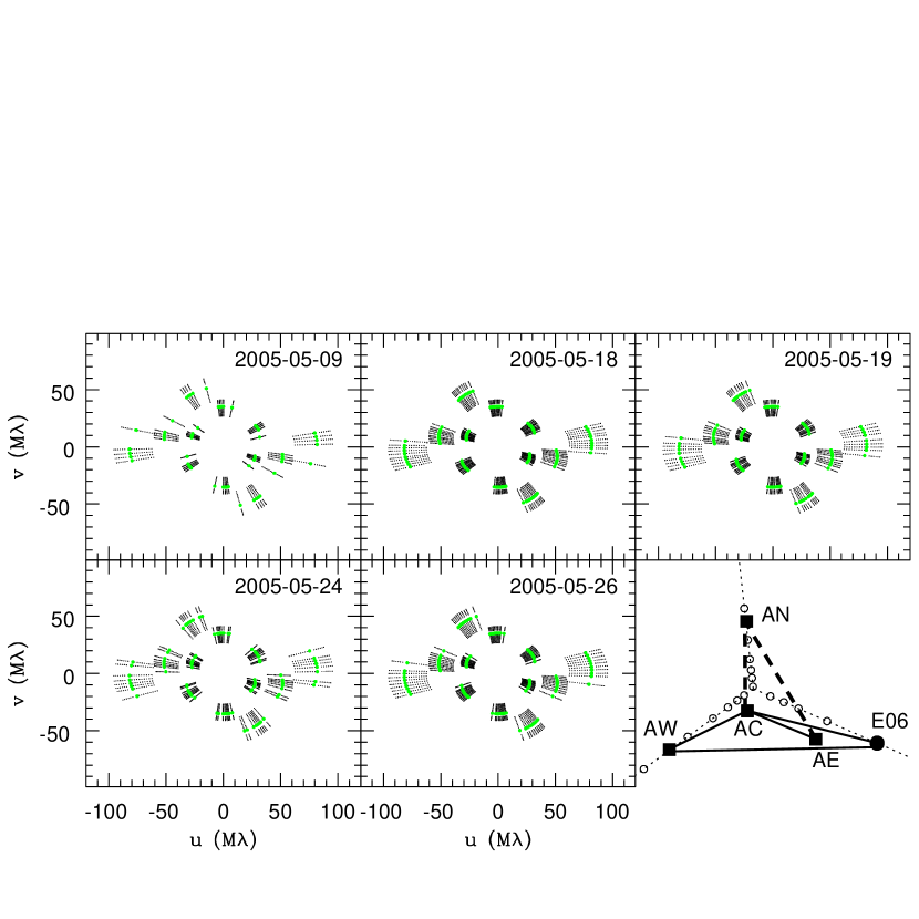
Figure 1: The $u-v$ coverage of the different nights. The black points show the continuum channels, while the green ones show H$\alpha$. The observing date is presented in the top right corner of each panel. The bottom right corner of the figure shows the array layout. The astrometric stations are shown as black squares and E06 is shown as a black dot. We also show the baselines used all nights as solid lines and the baselines that were used only on some nights, those involving AN, as dashed lines. The maximum baseline lengths can be found in Table 1.

Our observations were taken with the NPOI (Armstrong et al., 1998) on five different nights between 2005 May 09 and 2005 May 26. The observations were made with two spectrographs, simultaneously recording fringes in 16 spectral channels in the wavelength range 560–860 nm. Between one and three baselines were measured with each spectrograph. The maximum baseline lengths ranged from 18.9 to 53.3 m. In Table 1 we present a log of the observations, including the number of scans observed each night, the baselines used and the range of hour angles covered by the observations. Figure 1 presents the $(u,v)$-plane coverage achieved by the observations on each night. For reference, this figure also shows the array layout with the stations and baselines used. The observations of $\beta$ Lyrae were interleaved with observations of a nearby calibrator star $\gamma$ Lyrae (B9III, $V=3.24$ mag), which has a similar spectral type and magnitude to that of $\beta$Lyrae. Each calibrator or source scan had a duration of 30 s.

Throughout this paper we will use orbital phases of $\beta$ Lyrae based on the latest ephemeris of primary eclipses from Kreiner (2004). We assumed a single orbital phase for each night, corresponding to the midpoint of the observations (Table 1). This assumption will have no effect on the final results of this paper, because our observations usually lasted for $\sim$2 hours, which corresponds to $\sim$0.6% of an orbital period. Comparing the values obtained from this ephemeris with those from Harmanec & Scholz (1993) we find that the two predictions agree at the 2% level, which is sufficient for the purposes of the analysis presented here. As a final check, we compared the predicted times of minima with visual measurements from AAVSO, spread over a period of 2 months around our observations. We used only validated observations available at the AAVSO site and got an agreement better than 0.25 days between the observed and predicted minima, which corresponds to $\sim$2% of the orbital period.

The initial data reductions followed the incoherent and coherent integration methods described in Peterson et al. (2006a). In the case of the incoherent integration we start with data that were processed to produce squared visibilities ($V^{2}$) averaged into 1 s intervals. These data are then flagged to eliminate points with fringe tracking and pointing problems (Hummel et al., 1998, 2003a). The flagged data set is then used to bias correct the $V^{2}$ data, which are then calibrated. The calibrated $V^{2}$ values are later used to estimate the amplitudes of the complex visibilities.

For the coherent integration of complex visibilities, we use the technique presented by Hummel et al. (2003b) (see Jorgensen et al. 2007 for a different algorithm). We treat the visibilities in each 2 ms frame (the instrumental integration time) as phasors. To determine the phase shift from one fame to the next, we compute the power spectrum of the channeled visibility as a function of delay and measure the phase difference between the peak of the fringe envelope and the nearest fringe peak. We rotate the phasors to correct for this residual phase and average the complex visibilities in 200 ms subscans, which are used to determine the visibility phases. In Section 3, we describe other corrections applied to these data in order to obtain H$\alpha$ differential phases for $\beta$ Lyrae.

2.2 Spectroscopy

To estimate the strength of the H$\alpha$ emission in the $\beta$ Lyrae system, we have obtained a high resolution spectrum using a fiber-fed Echelle spectrograph at the Lowell Observatory’s John S. Hall telescope. The spectrum was acquired on 2005 May 19, which corresponds to the middle of our interferometric run. The spectroscopic data were processed using standard routines developed specifically for the instrument used in the observations (Hall et al., 1994). The final reduced spectrum in the H$\alpha$ region reaches a resolving power of 10,000 and signal-to-noise ratio of few hundred (see Fig. 2).

We obtain an equivalent width (EW) of $-1.5\pm 0.05$ nm for the H$\alpha$ profile shown in Figure 2. Most of the uncertainty in the EW measurement is due to the uncertainty associated with continuum normalization, which is estimated to be of the order of 3%. To obtain the total emission in the H$\alpha$ line we also need to correct for the underlying stellar absorption line that has been filled in by the emission from the circumstellar material. We estimate the EW of the underlying absorption line using the calibration developed by Coté & Waters (1987). Using a reddening corrected color $(B-V)_{0}=-0.05$ mag for $\beta$ Lyrae from Dobias & Plavec (1985), we obtain an EW of 0.72 nm for the H$\alpha$ absorption component, and therefore we estimate that the EW of the total H$\alpha$ emission is $-$2.2 nm. Considering that the NPOI H$\alpha$ channel has a width of $15\pm 1$ nm and the total emission line width is $-2.2$ nm, we derive a fractional contribution from the stellar photosphere ($c_{cnt}$) to the total flux in the channel of $0.87\pm 0.01$.

3 Differential phases

The challenge of recovering phase information from optical interferometric observations results from atmospheric and instrumental effects changing the phase calibration on a time scale of a few milliseconds. Fringe tracking can reduce these variations but not to the level needed for good imaging. Even with fringe tracking, the solution starts with 1) short exposures that freeze the fringe motion, 2) software that measures and removes these variations and 3) a coherent integration of hundreds of milliseconds (or more) needed to increase the signal to noise to a level sufficient for the rest of the data processing. The result is measurements of the real and imaginary parts of the visibility. The uncorrected phase variations during the coherent integration consist of a constant part and zero-mean fluctuations. The fluctuations reduce the measured visibility amplitude but have no effect on the phase. Thus these visibility data can be processed using closure relationships or self-calibration.

However, with a small number of stations, there are significantly more baselines than closure phases, so a significant fraction of phase information is lost. By contrast, the differential phase technique described here provides good phase information for every baseline. The idea is to recognize that the observed phase consists of three terms, viz. the desired source phase $\phi_{0}$, and offsets caused by the atmosphere and the instrument:

$$\phi_{obs}=\phi_{0}+\phi_{atm}+\phi_{inst}~{}.$$ (1)

All terms have implicit wavelength dependencies. The differential phase technique consists of 1) measuring $\phi_{obs}$ at several wavelengths, 2) modeling the three right-hand-side terms in Equation 1 and 3) deriving parameters of the model by fitting it to the measured $\phi_{obs}$. For the NPOI, $\phi_{inst}$ is stable and can be estimated by observing calibration stars; no parameters need to be fit. The atmospheric term, $\phi_{atm}$, is given by

$$\phi_{atm}=a(n-1)k+dk+\phi_{c}~{},$$ (2)

where $a$ is the differential air path between two beams, $n$ is the refractive index of air, $k$ the wavenumber $(2\pi/\lambda)$, $d$ the vacuum path difference and $\phi_{c}$ a wavelength independent phase offset (Jorgensen et al., 2006). Three quantities need to be fit: $a$, $d$, and $\phi_{c}$. Thus with at least four spectral channels, some information about the source can be obtained for each baseline.

3.1 Instrumental and Atmospheric Corrections

The H$\alpha$ emitting circumstellar disks of Be stars constitute one of the best cases for which one can calculate instrumental and atmospheric corrections to the visibility phases. This correction is based on observations of calibrator stars and the continuum channels of the star of interest. Since the photospheres of these stars usually do not deviate significantly from point symmetry, we can model the continuum as having zero intrinsic phase. Even in the case of rapidly rotating stars, in which the stellar image may deviate from point symmetry, the phase should vary smoothly and slowly with wavelength (Yoon et al., 2007; Peterson et al., 2006a, b). The same principle applies to calibration stars. These properties allow one to use the information from the continuum channels to calculate the appropriate corrections to the phases and interpolate them over the channel containing the H$\alpha$ line.

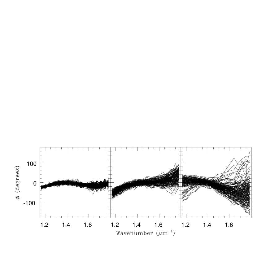
Figure 3: Coherently integrated phases of 3 scans of $\gamma$ Lyrae, one per panel, observed on 2005May09 with baseline AW0-E06. Each line corresponds to a different 200 ms subscan.

A first example of the instrumental and atmospheric effects on the phases of a partially resolved star is shown in Figure 3. Each panel of this figure shows a different scan of $\gamma$ Lyrae, while the different lines in each panel represent individual 200 ms subscans. Notice that the lines of the different subscans follow a similar cubic-like shape as a function of wavenumber, with some scatter. This cubic curve can be explained as an instrumental phase, due to uncompensated amounts of glass along the different beams. This curve does not change significantly from scan to scan, or from night to night. A further inspection of this figure shows that, besides this cubic component, one can also see a significant variation of the phase among different subscans. These variations are due to the differential air path between the two beams, and the shape of the curve is due to the fact that $(n-1)$ has a significant dependence on $k^{2}$ (Owens, 1967). One can also see in Figure 3 that the scatter is much smaller in the left panel, during the first scan of the night, increasing significantly toward later times (right), consistent with the worsening of the seeing conditions through the night.

In order to obtain differential phases of Be stars, one needs to correct the data for the two components described above. For the instrumental phases we use the values determined by averaging all the 200 ms subscans of calibrator stars observed throughout the night. Since the effects of the differential air path and vacuum delay are additive, one can reasonably assume that they should average down to zero over the course of a night. Also, since calibration stars are expected to have zero phase in the spectral range covered by our observations, by averaging the complex visibilities of the calibrators one is left only with instrumental phases, which can then be subtracted from the program star visibilities.

We demonstrate the procedure used to obtain instrumental phases in Figure 4. Here we show the phases obtained by averaging the visibilities of all subscans of $\gamma$ Lyrae observed on a night, 720 in total. We can also show that the other component affecting the phases of the subscans is due to differential air path between the two beams. Following the derivation presented by Armstrong et al. (1998), we expand Eq. 2 into a power series around $k_{0}$ and rewrite Eq. 1 in the following form:

$$\phi_{obs}=\phi_{0}+\phi_{inst}+c_{0}+c_{1}k+c_{2}k^{2}.$$ (3)

Starting from this equation and assuming that $\phi_{0}=0$, one can then solve for the coefficients $c_{0}$, $c_{1}$ and $c_{2}$ for each subscan, such that the residuals produce the best fit to the atmosphere phases ($\phi_{obs}-\phi_{inst}$). We show in Figure 4, as black lines, all subscans after subtracting only the atmosphere effects from the observed phases. Notice that these lines follow the instrumental one, with an r.m.s. of 0.15^∘ in the red and $\sim$0.5^∘ in the blue.

3.2 Differential Phases of $\beta$ Lyrae

The correction steps applied to the data of the program star ($\beta$ Lyrae) to obtain the phase in the H$\alpha$ channel are presented in Figure 5. In order to simplify the procedures and reduce the number of calculations, we take advantage of the fact that the atmospheric effects constitute an additive phase term, so instead of dealing with individual 200 ms subscans we can work with the average of all visibilities in a scan. The left panel of Figure 5 shows the average phases of nine scans of $\beta$ Lyrae. In the central panel we show the phases of the individual scans after the subtraction of the instrumental phase, shown as a dashed line in the left panel. The last step of the process is the correction of the atmospheric effects, by fitting a quadratic function of the form of Eq. 3 to the continuum channels for each average scan and subtracting the resulting function from all the channels.

In the procedures described above, the continuum phases of $\beta$ Lyrae were assumed to be zero. Nevertheless, one should expect to see phase variations across the spectrum. $\beta$ Lyrae is a binary system with a maximum separation of $\sim 1$ mas and $\Delta m\sim 0.9$ mag, with almost no color difference between the two components (Wilson, 1974; Harmanec, 2002). Using Eq. 8 of Mourard et al. (1992), we calculate that this system, observed at maximum separation with a 50 m baseline aligned with the separation vector, should show a continuum phase $\phi_{cnt}$ at the H$\alpha$ channel of $\sim 14^{\circ}$, with a slope of $1^{\circ}$ per channel. This case corresponds to the longest baseline in our data, but most of our baselines were 34 m long or less. For a 30 m baseline, $\phi_{cnt}$ at H$\alpha$ is $1.6^{\circ}$ with a slope of $0.2^{\circ}$ per channel.

Although the continuum phase component varies smoothly with wavenumber and can be modeled by our atmospheric phase subtraction method, arbitrarily setting this component to zero can in principle influence our results. The complex visibility of the H$\alpha$ channel results from the sum of the complex visibility of the continuum and H$\alpha$ emission line. Setting the continuum phase to zero will change the phase of the emission line visibility by $\phi_{cnt}$. For baselines of 30 m or smaller this is not an important effect, given the small continuum phases. However, as shown above, in the case of our longest baseline this can change the H$\alpha$ emission phase by as much as $\sim 14^{\circ}$. We discuss in Section 4 how we tested the effect of this assumption on the imaging of this source.

Figure 6 shows the differential phases of $\beta$ Lyrae on all baselines observed on 2005 May 19. Here we see results similar to those from Figure 5, with the continuum phases around zero, and the H$\alpha$ and He I channels showing a differential phase. The strongest H$\alpha$ phase is found on baselines with the longest extent along the E-W direction, with very little differential phase signals on baselines AN0-AC0 and AE0-AN0. Comparing these results with the ones from Mourard et al. (1992) and Harmanec et al. (1996) we get a consistent picture for this system. Based on GI2T observations, Harmanec et al. (1996) concluded that the orbit of the binary component should be roughly oriented along the E-W direction, since their observations used a N-S baseline and did not resolve the two stars. On the other hand, their line observations detected smaller $V^{2}$’s for H$\alpha$ and He I indicating that the line emitting region is more extended along the N-S direction. This result is consistent with the spectropolarimetric observations from (Hoffman, Nordsieck & Fox, 1998), who found that H$\alpha$, He I 587.6 nm and ultraviolet ($\lambda<360$nm) emission are polarized along p.a. $\sim 74^{\circ}$. This result indicates that this emission is polarized by a structure perpendicular to this direction. Another result that confirms this geometry is a radio nebula along p.a. $156\pm 4^{\circ}$ detected by Umana et al. (2000).

Comparing our results to those from Harmanec et al. (1996) suggests a possible contradiction, since we do not see a strong differential phase on the baselines oriented closer to the N-S direction, at least when comparing their signal to that measured on baselines oriented closer to the E-W direction. However, our observations can be explained in a way that agrees with the previous results. First, the weaker phase signal along the N-S direction can be explained in part as an effect of the baseline lengths of the two observations. Harmanec et al. (1996) used a baseline of 51 m, while for our AE0-AN0 baseline we have a longest projected length of only $\sim 25$ m along the N-S direction. Our maximum baseline length along the E-W direction is roughly twice that, which can explain the stronger differential phase signal along this direction. Second, we interpret the differential phases as a displacement between the H$\alpha$ line emitting region and the continuum photocenters. Since the binary system is expected to be oriented along the E-W direction, this would explain the stronger H$\alpha$ differential phases on baselines aligned closer to this direction.

Further support for this interpretation is presented in Figure 7, where we show the differential phases of baseline AW0-E06 on 2005 May 19 and 2005 May 26. These observations correspond to orbital phases of 0.24 and 0.78, respectively. Here we can see that the H$\alpha$ phase signal changes from negative to positive between the two dates, which can be understood as the center of line emission and continuum photocenter changing orientation relative to each other.

We would also like to point out another interesting result from Figure 6, the variation of the He I differential phases near $k\sim 1.4$ and $1.7~{}\mu$m^-1, in particular on baselines AE0-AC0 and AN0-AC0. One can see in this figure that the He I channel phases vary significantly from scan to scan, with the sign of the phase changing from positive to negative in a few scans. When we compare this behavior to that of the H$\alpha$ phases we see that H$\alpha$ does not change sign on the same night. This result indicates that the He I emitting region has a structure different from that of the H$\alpha$ region. This conclusion is supported by the spectropolarimetric results from Hoffman, Nordsieck & Fox (1998), who found that He I 587.6 nm and 706.5 nm have a different polarization properties from those of H$\alpha$ and He I 667.8 nm. This difference is due to the way these lines are excited, with the 587.6 ($k=1.70~{}\mu$m^-1) and 706.5 nm ($k=1.42~{}\mu$m^-1) being produced in higher density regions, possibly in the inner accretion disk.

4 Imaging

The ultimate goal of our differential phase experiment is the recovery of complex visibilities of this star in order to image the H$\alpha$ and continuum emission. In order to do this we start by combining the final phase information described above with the calibrated $V^{2}$’s from the incoherent integration method to calculate the corresponding complex visibilities for both continuum and line channels. Since these visibilities have been corrected for instrumental and atmospheric effects, the continuum channels can be exported into a FITS file and imaged using the usual radio interferometry techniques. However, in order to image the H$\alpha$ emission one needs to take into account the fact that most of the light in this channel originates from the continuum.

The correction for the continuum contribution to the H$\alpha$ channel is calculated using the $c_{cnt}$ value obtained from the spectroscopic measurements. Rewriting Eq. 1 of Tycner et al. (2006) in a more general form, we have the following relation for the continuum subtracted H$\alpha$ complex visibility:

$$V_{{\rm H}\alpha}=(V_{obs}-c_{cnt}V_{cnt})/(1-c_{cnt}).$$ (4)

$V_{obs}$ is the observed complex visibility in the H$\alpha$ channel, including the line and continuum components, $V_{cnt}$ and $V_{{\rm H}\alpha}$ are the complex visibilities of the continuum and H$\alpha$ components, and $c_{cnt}$ is the fractional contribution from the stellar continuum to the total flux in the H$\alpha$ channel. We use the average of the two channels adjacent to H$\alpha$ to estimate $V_{cnt}$ at the H$\alpha$ channel.

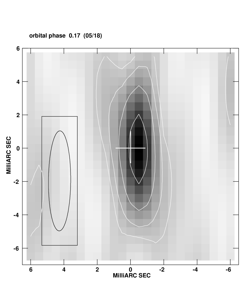
Figure 8: The following 5 figures show the H$\alpha$ images of $\beta$ Lyrae. Each figure corresponds to a different night and are organized in order of increasing orbital phase, indicated at the top of the panel. The cross shows the photocenter of the system, measured on the continuum images. The lowest contour corresponds to the 3$\sigma$ level. The reconstructing beam size and orientation is shown in the bottom left corner of each panel.

The resulting visibilities are converted into FITS files (one per night) and imaged using AIPS (van Moorsel, Kemball & Greisen, 1996). The resulting H$\alpha$ images are presented in Figure 8. These images were created using pixel sizes of 0.5 mas and a hybrid weighting scheme between natural and uniform weights, with robustness index 0. Just for reference we show in each panel, as a white cross, the position of the continuum photocenter, measured on continuum images restored from data observed on the same night. The position of the continuum was always in the center of the image, consistent with the fact that the continuum phases were set to $\sim 0^{\circ}$ in our procedures. Notice that in most cases the H$\alpha$ emission has a shape similar to that of the restoring beam, which indicates that the emission is unresolved, or just partially resolved, with a size comparable to that of the beam.

The most important result to be taken from Figure 8 comes from the comparison between the peaks of the H$\alpha$ and continuum emission. We can see in the different panels that these two points do not coincide, and that the displacement of the H$\alpha$ photocenter changes relative to that of the continuum as a function of orbital phase. Since the H$\alpha$ emission originates in the disk around the more massive star, while the continuum photocenter is located closer to the less massive one (Harmanec et al., 1996), we are effectively imaging the orbit of this system.

We also tested the effect introduced in the H$\alpha$ images of assuming that the continuum phase on the longest baseline is zero. To solve for this effect, we added 14^∘ to the phases of both H$\alpha$ and adjacent continuum channels of the longest baseline before subtracting the continuum contribution to the H$\alpha$ channel. We did not try to apply this correction to other baselines because of the small magnitude of their continuum phases. We followed the procedure described above and obtained new images using the uncorrected short baseline H$\alpha$ visibilities and the corrected long baseline H$\alpha$ visibilities. We do not find a significant change relative to the images obtained setting the continuum phase to zero. The position of the peaks of emission changed less than $0.4\sigma$, indicating that setting the continuum phases to zero was a reasonable approximation in this case.

5 The Orbit of $\beta$ Lyrae

Although we do not resolve the stars in this binary, our results can be used to derive some properties of the $\beta$ Lyrae system. First, since this is an eclipsing binary, it is straightforward to determine the orientation of the system on the plane of the sky. The inclination of the orbit is $86^{\circ}$ (Linnell, Hubeny & Harmanec, 1998; Linnell, 2000) and its projection on the sky can be reasonably well approximated by a straight line. In Figure 9 we show the position of the H$\alpha$ emission relative to the continuum photocenter for the five nights of data used in this paper. These positions were obtained by fitting gaussians to the images, and the values are given in Table 2.

Figure 9 also shows the orbit of the system, obtained by fitting a line with instrumental weighting ($1/\sigma^{2}$) to the data points. We find that the orbit is oriented along p.a.$=248.8\pm 1.7^{\circ}$. Notice that the point from 2005 May 18 has a much higher uncertainty in the N-S direction and deviates a little from the line. The uncertainty is caused by the fact that station AN0 was not used on this night, resulting in poorer resolution along this direction. We also point out that the fitted line does not cross the origin, which can be attribute to the fact that our observations cover only one half of the orbit, from orbital phases 0.17 to 0.78.

The reliability of the orbital orientation we obtain for the $\beta$ Lyrae system can be checked through the comparison with other measurements available in the literature. The radio observations presented by Umana et al. (2000) detected a jet-like nebular structure oriented along p.a.$=156.5\pm 4^{\circ}$. This nebula is perpendicular, within uncertainties, to the orbit p.a. derived here, agreeing with the expectation that jets are launched perpendicular to their disks. Further evidence confirming the orbital orientation of this system comes from the comparison of our results with the spectropolarimetric results of Hoffman, Nordsieck & Fox (1998). They predict that the jets should be oriented along p.a.$\sim 163.5^{\circ}$, similar to that found by Umana et al. (2000) and roughly perpendicular to the orbital orientation we found.

Finally, we compare our measurements of the displacement between the H$\alpha$ and continuum photocenters to predictions based on parameters of the system derived by others (e.g., Harmanec et al. 1996; Harmanec 2002; Linnell 2000). We use the same reference system as that of Harmanec et al. (1996), where the orbit is in the $X$-$Y$ plane, with the origin at the most massive star (the one which is currently gaining mass) and the $X$-axis is defined by the line joining the two stars. The analysis of the radial velocities of this system shows that the eccentricity of the orbit is 0 (Harmanec & Scholz, 1993). According to Harmanec (2002), the separation between the centers of the two stars is $58.52R_{\odot}$. For $\Delta m=0.9$ mag the position of the photocenter is at $X=40.64R_{\odot}$ and $Y=0$. Based on the analysis of the velocity curve of the H$\alpha$ emission Harmanec et al. (1996) found that this emission line originates in the disk ($X=4.12R_{\odot}$ and $Y=4.97R_{\odot}$), in a region offset from the center of the system, possibly related to the point of impact of the gas in the disk.

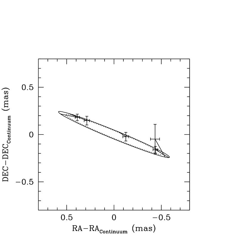
Figure 10: Same as Figure 9, but displaying the orbit calculated using the parameters described in Section 5 (solid line). The dotted line shows the orbit obtained if we assume that the system is at a distance of 309 pc, corresponding to a 1 $\sigma$ deviation in the distance. The lines connecting the points to the orbit indicate the expected position of the star in the model.

We used these parameters to calculate the orbits of the H$\alpha$ and continuum photocenters, and converted them to positions in the sky using the inclination derived by Linnell, Hubeny & Harmanec (1998) ($i=86^{\circ}$), the orientation derived by us (p.a.$=248.8^{\circ}$) and a distance of $270\pm 39$ pc. The resulting H$\alpha$ orbit relative to the continuum photocenter is shown in Figure 10. Here we can see that the orbit has the correct orientation, but has slightly larger semimajor axis than the one measured by us. The maximum calculated separation between the H$\alpha$ and continuum is 0.623 mas, which is $\sim 34$% larger than the value we measured (0.466 mas at orbital phase 0.24).

The difference between the observed and predicted orbital semimajor axis can be due to several effects. First, the uncertainty in the distance of this system is fairly large (39 pc). Increasing the distance of this source to 309 pc (corresponding to one standard deviation in the distance), the apparent size of the orbit is reduced by 14%. To illustrate this effect we show in Figure 10 (as a dotted line) the orbit obtained using a distance of 309 pc. The uncertainty in the $\Delta m$ of this system can also introduce errors in the size of the orbit. If we assume $\Delta m=0.8$mag instead of 0.9 mag, we get that the photocenter is at $X=39.48R_{\odot}$ and $Y=0$, which reduces the orbit size by $\sim 3$%.

Another important source of error in our measurements is the correction of the continuum contribution to the H$\alpha$ channel. Factors that contribute to errors in this correction are the uncertainty in the width of the channel and the EW of the H$\alpha$ absorption component. In this paper we used the Coté & Waters (1987) calibration to correct for the underlying H$\alpha$ absorption. However, their calibration is based on main sequence stars and may be overestimating the correction for $\beta$ Lyrae, where the brightest component is a B6-8II star. We tested this hypothesis by using the extreme assumption that the EW correction for the underlying absorption to H$\alpha$ is 0, which gives $c_{cnt}=0.91$. Using this value, we obtained new images and measured the position of H$\alpha$ emission relative to the continuum photocenter. The new measurements are shown in Figure 11, where we can see a result opposite to the one in Figure 10. In this case the observed semi major axis is 0.8 mas at orbital phase 0.24, $\sim 28$%, or larger than the predicted value.

6 Comparison Between Differential Phase and $V^{2}$ Results

As a way to check the results obtained with the differential phase technique, we use the calibrated continuum $V^{2}$ and closure phases to obtain information about the binary system. These measurements are used to compute the separation $\rho$ and position angle $\theta$ of the binary for each night. The best fit values, which were obtained for $\Delta m(670~{}nm)=0.9$ mag and assumed to be the same at other wavelengths, are given in Table 3 and plotted in Figure 12. This figure shows that the maximum separation between the two stars is of the order of $\sim 0.9$ mas, although with large uncertainties. Part of these uncertainties are related to the fact that our observations do not fully resolve this system, as can be seen in Figure 13. Here we present, for each night, the $V^{2}$’s of one scan observed with the longest baseline (AW0-E06, 53 m), and the corresponding best fitting models. We selected the scans within 30 minutes of meridian crossing, which is close to the highest resolution achieved with this baseline. This figure shows some of the limitations of our measurements. We observe higher $V^{2}$’s on the night of May 9, when the system is at orbital phase 0.47, and lower $V^{2}$’s on the other nights, when the stars are closer to their maximum elongation. However, we do not see the characteristic cosine wave signature of a binary, which makes the determination of the separation of the two stars uncertain.

When comparing the results obtained from the V² analysis with the H$\alpha$ ones, we should keep in mind that the former correspond to the separation between the photocenters of the two stars, while the latter correspond to the separation between the H$\alpha$ and continuum photocenters. Consequently, we need to convert the H$\alpha$ measurements to the same reference frame as the continuum measurements. Following the discussion presented in Section 5 we have that the two stars are separated by 58.52 R_⊙, the continuum photocenter is located at 40.64 R_⊙ from the most massive star, calculated assuming $\Delta$m=0.9 mag, and for simplicity we can say that the H$\alpha$ photocenter is located at 4.12 R_⊙ from this star. These numbers indicate that the measured H$\alpha$ separation relative to the continuum photocenter at orbital phase  0.25 corresponds to only 62% of the real separation between the photocenters of the two stars. Converting the measurements presented in Figures 10 and 11, we have that the observed H$\alpha$ orbits correspond to separations in the range 0.75 to 1.28 mas between the two stars (the range of values corresponds to $c_{cnt}=$0.87 and 0.91, respectively). Considering the uncertainties, these values are in very good agreement with those from the V² analysis presented in Figure 12.

Another way to confirm the H$\alpha$ results is by comparing the orientation of the orbits derived from the two methods. A least squares fit to the data presented in Figure 12, using instrumental weighting, gives a major axis orientation along p.a.$=256.1^{\circ}\pm 17.7^{\circ}$. This value is slightly different from the one obtained from H$\alpha$ measurements, p.a. $=248.8^{\circ}\pm 1.7^{\circ}$, but they are still in agreement, given the uncertainties.

As a last check we used the method described by Tycner et al. (2005, 2006) to determine the size of the H$\alpha$ disk. We used the calibrated H$\alpha$ V²’s, corrected to eliminated the continuum contribution from the binary star to this channel. Following the results from Tycner et al. (2006) we decided to fit the H$\alpha$ V²’s with a gaussian model, which results in a disk with HWHM=0.60$\pm$0.10 mas (Figure 14). The gaussian HWHM is comparable to the Roche lobe radius of $\sim$0.52 mas (30.3 R_⊙ Harmanec 2002), and consistent with the orbit obtained using the two methods described above.

7 Summary

In this paper we presented the development of a differential phase technique using NPOI data. We described the methods used to correct the instrumental and atmospheric effects on the phases of $\beta$ Lyrae, which allowed us to recover the complex visibility of the H$\alpha$ channel. We also described the procedure used to correct the continuum contribution to the H$\alpha$ channel and successfully imaged the line emission of this system using standard interferometric techniques. We found that the major axis is oriented along p.a. 248.8^∘, consistent with previous spectropolarimetric measurements, radio and optical interferometry results. From the comparison between the observed position of H$\alpha$ relative to the continuum photocenter and values obtained from models, we find that our measurements indicate a semi major axis smaller than that predicted by the models. We suggest that the most likely causes for this discrepancy are a wrong distance, brightness ratio between the 2 stars and the uncertainty in the correction of the continuum contribution to the H$\alpha$ channel. We also found that the results obtained using the technique developed here are consistent with those obtained from a more traditional analysis that uses only V² measurements.

The technique presented here represents a major step in the process of obtaining images from optical interferometric observations. Due to several limitation, the most important being the rapid time scales in which the atmosphere changes, the phases of a source wrap around too fast. Consequently, this information is lost and one cannot apply the usual image reconstruction techniques employed in radio interferometry. By making some assumptions about the structure of the source, our technique allows us to recover this information and obtain images for the emission line channels. In the case of $\beta$ Lyrae this allowed us to measure the orientation and size of the orbit using the relative location of the H$\alpha$ and continuum photocenters. We also found that the HeI emission has a different structure from that of H$\alpha$.

Besides $\beta$ Lyrae we are also applying this technique to other Be systems. This will allow us to image their circumstellar disk, map structures and study in better detail the accretion flow and effects such as the ionization of the disk by a binary companion.

Figure 2: Normalized high resolution H$\alpha$ profile of $\beta$ Lyrae.

Figure 4: Comparison between the phases of individual subscans from Figure 3, corrected for atmospheric and vacuum delay effects, and the instrumental phase (white line), obtained by averaging all subscans of the calibrator star observed in this particular night. The uncertainty in the instrumental phase is 0.15^∘ in the red part of the spectrum, growing to $\sim 0.5^{\circ}$ in the blue.

Figure 5: The different correction steps applied to the data of $\beta$ Lyrae. The first panel (left) shows the average phases of each scan (solid lines) as for baseline E06-AC0, obtained on 2005May19. The dashed line shows the instrumental phases and the dotted vertical line shows the location of the H$\alpha$ channel. The middle panel shows the phases obtained after subtracting the instrumental contribution. The right panel shows the differential phases obtained after subtracting a quadratic function, which was fitted to the continuum points only. The uncertainty in the phases is of the order of 0.3^∘ in the red, 0.5^∘ at H$\alpha$, growing to 1^∘ in the blue.

Figure 6: Residual phases of $\beta$ Lyrae after correcting for the instrumental, atmospheric and vacuum differential delay effects. Each panel shows a different baseline, observed on 2005May19. The individual lines represent individual scan averages. The vertical dotted line indicates the wavenumber of H$\alpha$, while the dashed ones show the wavenumbers of HeI.

Figure 7: Comparison of the differential phases of the longest baseline AW0-E06 (53 m) on the nights of 2005May19 (left) and 2005May26 (right). The two observing nights are separated by approximately half an orbital period.

Figure 9: Position of the peak of H$\alpha$ emission relative to the continuum photocenter. For each point we give the position uncertainty, obtained by fitting a gaussian to the image of the source. Besides each point we also indicate the orbital phase and the date of the observations. The dotted line was obtained by fitting a least squares line to the data. Since $\beta$ Lyrae is an eclipsing binary, this line is a good approximation for the orientation of the orbit in the plane of the sky (PA=248.8$\pm 1.7^{\circ}$).

Figure 11: Same as Figure 10, but displaying the H$\alpha$ positions measured on images created using a larger correction for the continuum contribution to the H$\alpha$ channel (c${}_{cnt}=0.91$). For simplicity we show only the model where the binary is at a distance of 270 pc.

Figure 12: Separation of the two binary components, obtained by fitting the continuum V² data. For each point we give the uncertainty in the position of the separation of the two sources. Besides each point we also indicate the orbital phase and the date of the observations. The dotted line was obtained by fitting a least squares line to the data, which gives the orientation of the orbit in the plane of the sky (PA=256.1$\pm 17.7^{\circ}$).

Figure 13: Calibrated V²’s of $\beta$ Lyrae observed with the longest baseline, AW0-E06 (53 m). The respective nights and orbital phases are indicated inside the panels. In order to make the visualization of the plots easier each panel shows only one scan, corresponding to the one observed within 30 minutes of local meridian crossing. The solid lines show the best fitting model for the corresponding night.

Figure 14: Calibrated H$\alpha$ visibilities from the H$\alpha$ channel. The dashed line shows the continuum V² after the removal of the binary signature. The dotted line shows the best elliptical Gaussian model fitted to the data.

Table 1: Observations Log

Date	UT Range	Number of Scans	Baselines	Hour Angle	Orbital Phase
2005May09	9.63 …11.90	5	E6-AC, AW-E6, AW-AC, AE-AC, AN-AC, AE-AN	–1.50 …0.79	0.47
2005May18	9.85 …11.80	10	E6-AC, AW-E6, AW-AC, AE-AC	–0.67 …1.28	0.17
2005May19	9.58 …11.75	9	E6-AC, AW-E6, AW-AC, AE-AC, AN-AC, AE-AN	–0.89 …1.29	0.24
2005May24	9.08 …11.63	8	E6-AC, AW-E6, AW-AC, AE-AC, AN-AC, AE-AN	–1.10 …1.48	0.63
2005May26	8.98 …11.36	10	E6-AC, AW-E6, AW-AC, AE-AC, AN-AC, AE-AN	–1.04 …1.34	0.78

Note. — The maximum lengths of the baselines shown in Column 3 are: E6-AC 34.3 m, AW-E6 53.3 m, AW-AC 22.2 m, AE-AC 18.9 m, AN-AC 22.9 m, AE-AN 34.9 m. We always used AC as the referenec station.

Table 2: Displacement of the H$\alpha$ and Continuum Photocenters

UT Date	Orbital Phase	RA(H$\alpha$-Continuum)	DEC(H$\alpha$-Continuum)
		(mas)	(mas)
2005May09	0.47	–0.13 $\pm$ 0.03	–0.02 $\pm$ 0.05
2005May18	0.17	–0.44 $\pm$ 0.05	–0.05 $\pm$ 0.16
2005May19	0.24	–0.44 $\pm$ 0.03	–0.16 $\pm$ 0.04
2005May24	0.63	0.29 $\pm$ 0.03	0.15 $\pm$ 0.05
2005May26	0.78	0.39 $\pm$ 0.02	0.18 $\pm$ 0.03

Note. — The orbital phases were calculated based on primary eclipse ephemeris from Kreiner (2004)

Table 3: Binary Separations

UT Date	Orbital Phase	$\rho$	$\theta$	$\Delta_{Maj}$	$\Delta_{Min}$	$\phi$
		(mas)	(deg)	(mas)	(mas)	(deg)
2005May09	0.47	0.47	248.1	0.52	0.23	5.0
2005May18	0.17	0.85	261.5	1.09	0.19	177.9
2005May19	0.24	0.90	260.0	0.52	0.21	2.7
2005May24	0.63	0.78	76.7	0.51	0.23	3.8
2005May26	0.78	0.91	72.5	0.52	0.21	1.9

Note. — Column 1: date of the observations; Column 2: orbital phase; Columns 3 and 4: binary separation and position angle; Columns 5, 6 and 7: position uncertainty ellipse major axis, minor axis and position angle.

References

- Akeson, Swain & Colavita (2000) Akeson, R. L., Swain, M. R., & Colavita, M. M. 2000, Proc. SPIE, 4006, 321
- Armstrong et al. (1998) Armstrong, J. T., et al. 1998, ApJ, 496, 550
- Baldwin, et al. (1996) Baldwin, J. E., et al. 1996, A&A, 306, L13
- Coté & Waters (1987) Coté, J., & Waters, L. B. F. M. 1987, A&A, 176, 93
- Dobias & Plavec (1985) Dobias, J. J., & Plavec, M. J. 1985, AJ, 90, 773
- Goodricke & Englefield (1785) Goodriecke, J., & Englefield, H. C. 1785, Philosophical Transactions Series I, 75, 153
- Hall et al. (1994) Hall, J. C., Fulton, E. E., Huenemoerder, D. P., Welty, A. D., & Neff, J. E. 1994, PASP, 106, 315
- Harmanec (2002) Harmanec, P. 2002, Astronomische Nachrichten, 323, 87
- Harmanec et al. (1996) Harmanec, P. 1996, A&A, 312, 879
- Harmanec & Scholz (1993) Harmanec, P., & Scholz, G. 1993, A&A, 279, 131
- Hoffman, Nordsieck & Fox (1998) Hoffman, J. L., Nordsieck, K. H., & Fox, G. K. 1998, AJ, 115, 1576
- Hummel et al. (1998) Hummel, C. A., Mozurkewich, D., Armstrong, J. T., Hajian, a. R., Elias II, N. M., & Hutter, D. J. 1998, AJ, 116, 2536
- Hummel et al. (2003a) Hummel, C. A., et al. 2003a, AJ, 125, 2630
- Hummel et al. (2003b) Hummel, C. A., Mozurkewich, D., Benson, J. A., & Wittkowski, M. 2003b, SPIE, 4838, 1107
- Jorgensen et al. (2006) Jorgensen, A. M., et al. 2006, SPIE, 6268, 47
- Jorgensen et al. (2007) Jorgensen, A. M., et al. 2007, AJ, 134, 1544
- Kreiner (2004) Kreiner, J. M. 2004, Acta Astronomica, 54, 207
- Linnell (2000) Linnell, A. P. 2000, MNRAS, 319, 255
- Linnell, Hubeny & Harmanec (1998) Linnell, A. P., Hubeny, I., & Harmanec, P. 1998, ApJ, 509, 379
- Monnier (2003) Monnier, J. D., 2003, Reports of Progress in Physics, 66, 789
- Monnier et al. (2007) Monnier, J. D., et al. 2007, Science, 317, 342
- Morgan, Potter & Kondo (1974) Morgan, T. H., Potter, A. E., & Kondo, Y. 1974, ApJ, 190, 349
- Mourard et al. (1992) Mourard, D., et al. 1992, IAU colloq. 135: Complementary Approaches to Double and Multiple Star Research, 32, 510
- Owens (1967) Owens, J. C. 1967 Appl. Opt., 6, 51
- Perryman et al. (1997) Perryman, M. A. C., et al. 1997, A&A, 323, L49
- Peterson et al. (2006a) Peterson, D. M., et al. 2006, ApJ, 636, 1087
- Peterson et al. (2006b) Peterson, D. M., et al. 2006, Nature, 440, 896
- Quirrenbach (1999) Quirrenbach, A. 2000, in Principles of Long Baseline Stellar Interferometry, Ed. P. R. Lawson, p. 143
- Quirrenbach et al. (1994) Quirrenbach, A. Buscher, D. F., Mozurkewich, D., Hummel, C. A., & Armstrong, J. T. 1994, A&A, 283, L13
- Sahade et al. (1959) Sahade, J., Huang, S. S., Struve, O., & Zebergs, V. 1959, Transactions of the American Philosophical Society, 49, 32
- Tycner et al. (2005) Tycner, C. et al. 2005, ApJ, 624, 359
- Tycner et al. (2006) Tycner, C. et al. 2006, AJ, 131, 2710
- Umana et al. (2000) Umana, G., Maxtel, P. F. L. Triglio, C., Fender, R. P., Leone, F., & Yerli, S. K. 2000, A&A, 358, 229
- Vakili et al. (1997) Vakili, F., Mourard, D., Bonneau, D., Mourand, F., Stee, P. 1997, A&A, 323, 183
- Vakili et al. (1998) Vakili, F., et al. 1998, A&A, 335, 261
- van Moorsel, Kemball & Greisen (1996) van Moorsel, G., Kenball, A., & Greisen, E. 1996, in ASP Conf. Ser. 101, Astronomical Data Analysis Software and Systems V, ed. G. H. Jacoby & J. Barnes (San Francisco:ASP), 37
- Wilson (1974) Wilson, R. E. 1974, ApJ, 189, 319
- Yoon et al. (2007) Yoon, J. et al. 2007, PASP, 119, 437