Low-Luminosity Gamma-Ray Bursts as a Distinct GRB Population: A Firmer Case from Multiple Criteria Constraints

Abstract

The intriguing observations of Swift/BAT X-ray flash XRF 060218 and the BATSE-BeppoSAX gamma-ray burst GRB 980425, both with much lower luminosity and redshift compared to other observed bursts, naturally lead to the question of how these low-luminosity (LL) bursts are related to high-luminosity (HL) bursts. Incorporating the constraints from both the flux-limited samples observed with CGRO/BATSE and Swift/BAT and the redshift-known GRB sample, we investigate the luminosity function for both LL- and HL-GRBs through simulations. Our multiple criteria, including the $\log N-\log P$ distributions from the flux-limited GRB sample, the redshift and luminosity distributions of the redshift-known sample, and the detection ratio of HL- and LL- GRBs with Swift/BAT, provide a set of stringent constraints to the luminosity function. Assuming that the GRB rate follows the star formation rate, our simulations show that a simple power law or a broken power law model of luminosity function fail to reproduce the observations, and a new component is required. This component can be modeled with a broken power, which is characterized by a sharp increase of the burst number at around $L<10^{47}$ erg s^-1. The lack of detection of moderate-luminosity GRBs at redshift $\sim 0.3$ indicates that this feature is not due to observational biases. The inferred local rate, $\rho_{0}$, of LL-GRBs from our model is $\sim 200$ Gpc^-3 yr^-1 at $\sim 10^{47}$ erg s^-1, much larger than that of HL-GRBs. These results imply that LL-GRBs could be a separate GRB population from HL-GRBs. The recent discovery of a local X-ray transient 080109/SN 2008D would strengthen our conclusion, if the observed non-thermal emission has a similar origin as the prompt emission of most GRBs and XRFs.

1 Introduction

Long duration Gamma-ray bursts (GRBs) are believed to be tied to the death of massive stars (Colgate 1974; Woosley 1993; Stanek et al. 2003; Hjorth et al. 2003; Campana et al. 2006). Of the roughly 6000 bursts observed since the late 1960s (see e.g. http://heasarc.gsfc.nasa.gov/grbcat/), almost 100 have redshift measurements. Observations show that long GRBs are scattered over a large redshift and luminosity range, from $z=0.0085\sim$ 6.7 and $L=10^{46}\sim 10^{54}~{}{\rm erg~{}s}^{-1}$. Most of these bursts have high luminosity (HL, $L>$ several $10^{48}$ erg s^-1) with the exception of two peculiar bursts, GRBs 980425 and 060218, which have extremely low redshift and luminosity measurements, $(z,L)=(0.0085,4.7\times 10^{46}~{}{\rm erg~{}s}^{-1}$) and (0.033, 6.03$\times 10^{46}~{}{\rm erg~{}s}^{-1}$) respectively (Tinney et al. 1998; Mirabal et al 2006). It remains unclear whether the LL-GRBs are due to unusual progenitor properties or a unique population with an intrinsic difference in the central engine, i.e., black hole versus magnetar (Mazzali et al. 2006; Soderberg et al. 2006; Toma et al. 2007).

One empirical way to look into this problem is to see whether observational data collected so far are still consistent with LL-GRBs as a natural extention of HL-GRBs to low luminosities in a continuous luminosity function (LF), or if LL-GRBs form a distinct new LF component. We have suggested that the latter possibility (two-component LF model) is necessary based on the redshift-known sample of GRBs after the discovery of GRB 060218 (Liang et al. 2007). Such a possibility has also been considered as a hypothesis in the BeppoSAX era (Coward 2005). On the other hand, although Guetta & Della Valle (2007) agreed that the two-component model is possible, they also argued that the $z$-known GRB sample may be also consistent with a single component model with a steeper slope in the luminosity function so that more LL-GRBs are accounted for.

Comparing observational data with simulations is a useful way to address the relationship between LL-GRBs and HL-GRBs. It is an important task to constrain the luminosity function, $\Phi(L)$, and local rate of GRBs, $\rho_{0}$, in a manner that can self-consistently reproduce various observations. In particular, the current LL-GRB population studies have been focused on the $z$-known sample only. They were not confronted with the existing $\log N-\log P$ distribution of the BATSE GRB sample. The $\log N-\log P$ distribution (or $V/V_{\rm max}$ distribution) addresses the statistical properties of GRBs regardless of their redshift, and carries essential information of the GRB LF. For HL-GRBs, this criterion has been utilized extensively (e.g. Schmidt 2001; Stern et al. 2002; Lloyd-Ronning et al. 2002; Norris 2002; Guetta et al. 2005) and was confronted with simulations (Lloyd-Ronning et al. 2004; Dai & Zhang 2005; Daigne et al. 2006). The conclusion has been that $\Phi(L)$ of HL-GRBs is generally characterized by a one-component broken power law model with $\rho_{0,HL}\sim 1~{}{\rm Gpc^{-3}~{}yr^{-1}}$ (e.g. Schmidt 2001; Guetta et al. 2004, 2005). On the other hand, the $\rho_{0}$ of LL-GRBs inferred from the two detections (GRBs 980425 and 060218) in a decade suggests a much higher local rate than that of HL-GRBs, i.e., $\rho_{0,LL}=100\sim 1000$ Gpc^-3 yr^-1 (Coward 2005; Cobb et al. 2006; Pian et al. 2006; Soderberg et al. 2006; Liang et al. 2007; Chapman et al. 2007). Guetta et al. (2004) propose an extension to lower luminosities which would increase ${\rho_{\rm 0,HL}}$ from roughly $1.1~{}{\rm Gpc^{-3}~{}yr^{-1}}$ to $10~{}{\rm Gpc^{-3}~{}yr^{-1}}$, at roughly $10^{48}~{}{\rm erg~{}s^{-1}}$. This local rate, however, even extrapolated down to $10^{45}~{}{\rm erg~{}s^{-1}}$ is not sufficiently large to produce the observed LL events. This was the main motivation of the two-component model in our previous analysis (Liang et al. 2007, see also Coward 2005; Le & Dermer 2007). The analysis with the $z$-known sample makes an arguable case (Liang et al. 2007), but is by no means conclusive (cf. Guetta & Della Valle 2007).

In this paper we extend our previous analysis to include a more complete set of observational constraints. In particular, we introduce the important BATSE and Swift $\log N-\log P$ distribution criteria along with the previously considered multiple criteria involving the $z$-known sample (1-D $z$-distribution, 1-D $L$-distribution, 2-D $z-L$ distribution, and the observed number ratio of HL- vs. LL-GRBs). Although the number of LL-GRBs remains the same, the $z$-known sample has grown since our last analysis in Liang et al. (2007), a firmer conclusion drawn in this paper is largely due to the additional observational criterion included in this analysis. In order to confront multiple criteria with different LF models and a wide range of LF parameters, we utilize a series of Monte Carlo simulations (MCSs). Instrument observational selection effects are difficult to model, and we introduce some empirical formulae to roughly reflect gamma-ray detector trigger sensitivity and the selection effect of redshift measurement. Various models are presented in §2. Our siumlation results are shown in §3, and the conclusions and discussion are presented in §4. The concordance cosmology with parameters $H_{\rm 0}=71$ km s^-1 Mpc^-1, $\Omega_{\rm{m}}=0.3$ and $\Omega_{\Lambda}=0.7$ is assumed throughout.

Throughout the paper we do not touch on another distinctly different group of bursts, namely short-hard (Kouveliotou et al. 1993), or more general Type I (see e.g. Zhang et al. 2007 for a discussion of the multiple criteria needed to classify GRBs) bursts, which are found to be consistent with the compact-star-merger origin (Gehrels et al. 2005; Fox et al. 2005; Barthelmy et al. 2005; Berger et al. 2005c, see Mészáros 2006, Nakar 2007, Zhang 2007 for reviews). The analysis of these GRBs applying the same technique will be presented elsewhere.

2 Models

2.1 Number of detectable GRBs with an Instrument

Assuming that the GRB rate at redshift $z$ is $R_{GRB}(z)$ (number of GRBs per unit time per unit volume), the number of GRBs happening per unit (observed) time in a comoving volume element $dV(z)/dz$ is

$$\frac{dN}{dtdz}=\frac{R_{GRB}(z)}{1+z}\frac{dV(z)}{dz},$$ (1)

where the $(1+z)$ factor accounts for the cosmological time dilation, and $dV(z)/dz$ is given by

$$\frac{dV(z)}{dz}=\frac{c}{H_{\rm 0}}\frac{4\pi D_{L}^{2}}{(1+z)^{2}[\Omega_{M}(1+z)^{3}+\Omega_{\Lambda}]^{1/2}},$$ (2)

for a flat $\Lambda$CDM universe. The observed GRB/supernovae connection suggests that the GRB rate could roughly trace the star formation history. We adopt a parameterized GRB rate model proposed by Porciani and Madau (2000),

$$R_{GRB}=23\rho_{\rm 0}\frac{e^{3.4z}}{e^{3.4z}+22.0}.$$ (3)

or by Rowan-Robinson (1999),

$$R_{GRB}=\rho_{0}\left\{\begin{array}[]{l@{\quad\quad}l}10^{0.75z}&z<1\\ 10^{0.75z_{peak}}&z>1,\\ \end{array}\right.$$ (4)

where $z_{peak}$ is the redshift at which the redshift distribution reaches its maximum (after which it plateaus), taken here as 1.

Supposing the GRB luminosity function is $\Phi(L)$, the number of GRBs per unit time at redshift $z\sim z+dz$ and luminosity $L\sim L+dL$ is given by

$$\frac{dN}{dtdzdL}=\frac{R_{GRB}(z)}{1+z}\frac{dV(z)}{dz}\Phi(L).$$ (5)

Considering an instrument with energy band [$e_{1}$, $e_{2}$] having a flux threshold $F_{\rm th}$ and an average solid angle $\Omega$ for the aperture flux, the number of the detected GRBs during an observational period of $T$ should be

$$N=\frac{\Omega T}{4\pi}\int_{L_{1}}^{L_{2}}\Phi(L)dL\int_{0}^{z_{\max}}\frac{R_{\rm GRB}(z)}{1+z}\frac{dV(z)}{dz}dz,$$ (6)

where $z_{\max}$ for a given burst with luminosity $L$ is determined by the instrumental flux threshold $F_{\rm th}$ through $F_{\rm th}=L/4\pi D^{2}_{L}(z_{\max})k$. The $k$ factor corrects the observed flux in an instrument band to bolometric flux in the burst rest frame ($1-10^{4}$ keV in this analysis),

$$k=\frac{\int_{1/(1+z)}^{10^{4}/(1+z)}EN(E)dE}{\int_{e_{1}}^{e_{2}}EN(E)dE}.$$ (7)

where $N(E)$ is the photon spectrum of GRBs. It is generally fitted with a joined power law (the Band function; Band et al. 1993) characterized with photon indices $\Gamma_{1}$ and $\Gamma_{2}$ before and after a break at $E_{0}$. The peak energy of the $\nu f_{\nu}$ spectrum is given by $E_{p}=E_{0}(2+\Gamma_{1})$. It was shown that $\Gamma_{1}\sim-1$, $\Gamma_{2}\sim-2.3$, and $E_{p}\sim 250$ keV for a typical GRB (Preece et al. 2000). In our analysis, the luminosity extends over ten orders of magnitude ([$10^{45}$, $10^{55}$] erg $\rm s^{-1}$). According to the Amati relation (Amati et al. 2002; Liang et al. 2004), more luminous bursts have a higher $E_{p}$, indicating that we cannot adopt a uniform $E_{p}$ for all the bursts in our analysis. Liang et al. (2004) derived

$$E_{p}/200{\rm keV}=C(L/10^{52}{\rm erg\ s}^{-1})^{1/2}$$ (8)

where $C$ is randomly distributed in [0.1,1]. We obtain $E_{p}$ with Eq. 8 for each burst and assume $\Gamma_{1}\sim-1$ and $\Gamma_{2}\sim-2.3$ for all bursts.

With the spectral information, one can make the k-correction and get the observed peak energy flux and peak photon flux by

$$F=\frac{L}{4\pi D_{L}^{2}k}$$ (9)

and

$$P_{ph}=\frac{F\int_{e_{1}}^{e_{2}}N(E)dE}{\int_{e_{1}}^{e_{2}}EN(E)dE},$$ (10)

respectively.

2.2 Luminosity Functions

Attempts to determine $\Phi(L)$ of long GRBs have been made by some authors, through fitting the $\log N-\log P$ or $V/V_{\rm max}$ distributions observed by CGRO/BATSE (Schmidt 2001; Stern et al. 2002; Lloyd-Ronning et al. 2002; Norris 2002; Guetta et al. 2005), and generally characterize $\Phi(L)$ with a single power-law or an a broken power law within a given luminosity range [$L_{1}$, $L_{2}$], i.e.,

$$\Phi(L)=\Phi_{0}\left(\frac{L}{L_{B}}\right)^{-\alpha},$$ (11)

or

$$\Phi(L)=\Phi_{0}\left[\left(\frac{L}{L_{b}}\right)^{\alpha_{1}}+\left(\frac{L}{L_{b}}\right)^{\alpha_{2}}\right]^{-1},$$ (12)

where $\Phi_{0}$ is a normalization constant to assure $\int_{L_{1}}^{L_{2}}\Phi(L)dL=1$. The local GRB rate, $\rho_{0}=R_{GRB}(z=0)$, is in principle defined to include GRBs with all luminosities. In practice, since observations cannot probe the full luminosity function, the $\rho_{0}$ value constrained by the data is usually related to a lowest luminosity $L_{1}$. The value of $\rho_{0}$, therefore, is a function of $L_{1}$. For a single power law LF (Eq. 11) with $\alpha>1$, one has $\rho_{0}(L>L_{1})\propto L_{1}^{-(\alpha-1)}$, suggesting that a lower $L_{1}$ would give rise to a larger observed $\rho_{0}(L>L_{1})$. For a broken power law LF (Eq.12) with $\alpha_{1}<1$ and $\alpha_{2}>1$, on the other hand, integration suggests that $\rho_{0}(L>L_{1})\sim\rho_{0}(L>L_{b})$ which is essentially independent of $L_{1}$. Thus fixing $L_{b}$ would usually fix $\rho_{0}$ in the broken PL models. In the past, the LF of HL-GRBs was found to have a break around $L_{b}\sim 10^{50}\rm~{}erg~{}s^{-1}$, with the value of $\rho_{0}$ related to $L_{b}$. In our analysis, the local rate is evaluated at a lower luminosity cutoff for all models, although the value is determined by either $L_{1}$ or $L_{\rm b,LL}$ depending on the forms of LF adopted. These are summarized in Table 1.

2.3 Instrument Threshold and Detection Biases

In order to check if a simulated burst is detectable with a given instrument, the simulated burst is screened with the instrument threshold. The CGRO/BATSE was triggered by energy-dependent count rate (Band 2003). We take a moderate sensitivity for CGRO/BATSE at 50-100 keV band as $F_{th}^{BATSE}\sim 10^{-7}$ erg cm ^-2 s^-1 , roughly corresponding to $0.2$ ph cm^-2 s^-1 for a typical GRB.

The BAT instrument on board Swift operates with an image trigger mechanism. The sensitivity of an event depends on many complicated factors and in principle should be treated in the case-by-case basis. For the purpose of this paper, we adopt an approximate formula of Sakamoto et al. (2007),

$$F_{th}\sim{(5.3\times 10^{-9}~{}\rm erg~{}cm^{-2}~{}s^{-1})}{f}^{-1}t_{90}^{-0.5}.$$ (13)

where $f$ is the partial coded fraction and $t_{90}$ is the burst duration. The larger the burst duration, the more sensitive the instrument. Bursts with $F>F_{th}$ can be in principle detected. Observationally, the “peak fluxes” (and therefore the “peak luminosities”) are usually adopted to denote for the brightness of the bursts, which are on average 5 times above the average fluxes (T. Sakamoto, private communication). To compensate this effect, we hereafter adopt an effective threshold condition which is 5 times larger than Eq.(13) in our peak-luminosity analyses. Since HL-GRBs have a typical duration of 20 s, we adopt a rough constant threshold flux of $F_{th,eff}\sim 1.2\times 10^{-8}~{}\rm erg~{}cm^{-2}~{}s^{-1}$ for the analyses of HL-GRBs. As shown by Norris et al. (2005), LL-GRBs tend to have longer pulse duration. GRB 060218, for example, has a duration longer than 2000 seconds (Campana et al. 2006; Liang et al. 2006). In our analysis we adopt various discrete values of BAT sensitivities, not exceeding a 500 second duration (i.e., $4.7\times 10^{-10}~{}\rm erg~{}cm^{-2}~{}s^{-1}$), to screen the simulated LL-GRBs.

Theoretically, a GRB could be detectable if $F>F_{th,eff}$. Note that a large fraction of detectable events with $F$ close to $F_{th,eff}$ may not trigger the instrument. This fact was observed in CGRO/BATSE. An off-line scan found a large number of non-triggered GRBs in the BATSE catalog, most of them are near the instrument threshold (Stern et al. 2001). Our simulations, by not adopting a threshold for the $\log N-\log P$ distribution have an advantage in deciphering the intrinsic low photon flux end of the distribution, which may be tested in the future by more seneitive detectors such as JANUS (Roming et al. 2008) and EXIST (Grindlay 2006).

In our analysis we also compare the simulated sample with the redshift-known GRB sample. This sample suffers many observational biases (Bloom et al. 2001; Butler et al. 2007), including position localization, optical detection, and line detection. The trigger probability of a burst with a flux close to the instrument threshold tends to be low, as seen in BATSE. Near-threshold GRBs tend to have fainter optical afterglows, which severely bias against their redshift measurements. It is difficult to fully incorporate all these biases into the simulation. We simply model the redshift detection probability of a simulated burst based on an empirical formula,

$$p(F)=(1-\frac{F_{th}}{F})^{\kappa},$$ (14)

where $\kappa$ is a free parameter. Our analyses show that $\kappa\sim 7$ is necessary to eliminate the overproduction of bursts near the sensitivity threshold. Equation 14 is not highly sensitive on the value of $\kappa$, whose most notable effect is on bursts near the threshold. As the value of $\kappa$ is decreased, most bursts appear near the threshold and below the band of observed bursts, significantly decreasing the significance of the correlation between the simulated and observed bursts. We notice that the correlation between gamma-ray and optical luminosities is not a strong one (e.g. Liang & Zhang 2006; Nardini et al. 2006; Kann et al. 2007; Nysewander et al. 2008), and that determination of redshift is easier in some ranges than others. All these make the selection effects more complicated than the simple parameterization such as Eq.14. Nonetheless, without simulating the optical luminosities, here we take a simple form for the sake of simplicity, which can effectively screen low-luminosity bursts without affecting the bursts significantly above the threshold.

3 Monte Carlo Simulations Against Observations

We place constraints on the parameters of $\Phi(L)$ and $R_{GRB}$ through comparing our simulations with observations. The primary criterion to judge the parameters is that the simulated $\log N-\log P$ distribution should match the data. The detection number of an instrument in a given observation period should roughly match the observations. CGRO/BATSE and Swift/BAT established two uniform samples that can constrain the parameters with the detection event number and the fits to the observed $\log N-\log P$ distributions. The size of the mock GRB sample for a given instrument accumulated in a period $T$ is obtained with Eq. 6. CGRO/BATSE recorded 1637 triggered long GRB events during 9.1 operation years (4B catalog, Paciesas, et al., 1999), and Swift/BAT was triggered by $\sim 300$ GRBs during the first 3 years of operation. We regard all detectable type II GRB events that could trigger BAT. Therefore, a set of the parameters can be obtained by adjusting the parameters that makes the detectable event numbers with BATSE and BAT could be $2176$ events in $9.1$ years (1393 triggered and 874 non-trggered) and $N=300$ in $3$ years, respectively, and the observed $\log N-\log P$ with the two instruments that match our simulations. We measure the consistency between observations and our simulations by a K-S test, resulting in a probability $p_{\rm K-S}$ (Press et al. 1997). The larger $p_{\rm K-S}$ suggests a more significant consistency.

The second criterion to judge the parameters is the constraints from the redshift-known sample and the detections of LL-GRBs. The current GRB sample with redshift measurements has $\sim 100$ GRBs, and only two confirmed detections of LL-GRBs. They were detected by different instruments. Although the sample is not homogeneous for statistics, the parameters of $\Phi(L)$ and $R_{GRB}$ are subject to the constraints from this sample, especially when we take the LL-GRBs into account (Liang et al. 2007). First, the detection ratio of LL-GRBs to HL-GRBs should be $\sim 1:300$ as observed by BAT in three years. Second, both the simulated one-dimensional distributions of $L$ and $z$ and the GRB distribution in the $(L-z)$ plane should roughly match the observations. We therefore simulate a sub-sample of GRBs that have redshift measurement based on the probability of redshift measurement (Eq. 14) from simulated GRB sample for BAT. We measure the one-dimensional $L$ and $z$ distribution with the K-S test, and then combine the distributions in order to place more rigorous constraints. We compare two-dimensional contributions in the $L-z$ plane and measure the consistency of the simulated sample to the observational data with $p_{\rm K-S,t}=p_{\rm K-S,L}\times p_{\rm K-S,z}$.

With the criteria described above, we adjust the model parameters and simulate a large sample of GRBs and filter them with a given instrument threshold without considering the cosmological evolution of $\Phi(L)$, stopping the simulations when a sub-sample of 150 detectable bursts are reached. Our simulation procedure is summarized as follows.

First, we simulate a burst that is characterized with $L$ at redshift $z$, GRB($L,z$). Both quantities are simulated separately with the probability distributions derived from Eq. 1 and $\Phi(L)$ (one of Eqs. 11-12).

Second, we calculate the $E_{p}$ of a mock GRB with Eq. 8, and its $F$ and $P_{ph}$ from Eqs. 9 and 10, respectively. The simulated GRB then is screened with the threshold condition $F>F_{th}$.

Third, we simulate a redshift-known sub-sample from the flux-cutoff mock sample with Eq. 14.

In each of the following subsections we will try different LF models and compare the simulations with the observations.

3.1 Simple Power Law Model

The first model considered is the simple power law model (Eq. 11). This scenario has been extensively studied with the BATSE data (see §1). Guetta et al. (2004) investigate this model without considering the LL-GRBs. In order to explain the high detection rate of LL-GRBs, Guetta & Della Valle (2007) proposed that the GRB luminosity function is a single PL with a slope $\alpha=1.6$ and $\rho_{0}=1.1$, 200, or (200-1800) Gpc^-3 yr^-1 depending on which lower luminosity cutoff was used, $5\times 10^{49}~{}\rm erg~{}s^{-1}$, $5\times 10^{47}~{}\rm erg~{}s^{-1}$, or $5\times 10^{46}~{}\rm erg~{}s^{-1}$, as summarized in Table 1. We make simulations with this model and adopt the parameters from Guetta et al. (2004, 2007). The simulated results of these models are shown in Figs. 1-4. We first compare the simulated results to the $\log N-\log P$ distribution observed by BATSE. In general, as far as HL-GRBs are concerned, the model is able to reproduce a good comparison to the $\log N-\log P$ (Fig.1 a,b). However, in order to accommodate LL-GRBs, modifications of the LF parameters are needed. The revised model (Guetta & Della Valle 2007), although able to account for the event rate of LL-GRBs, deviates from the observed BATSE $\log N-\log P$ distribution significantly (Fig.1c).

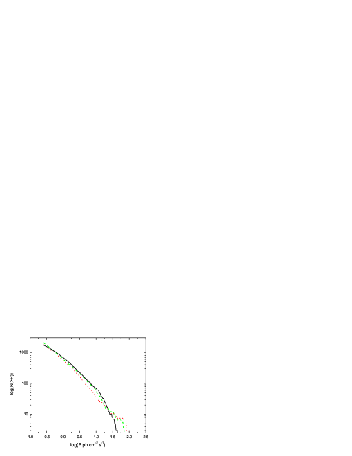
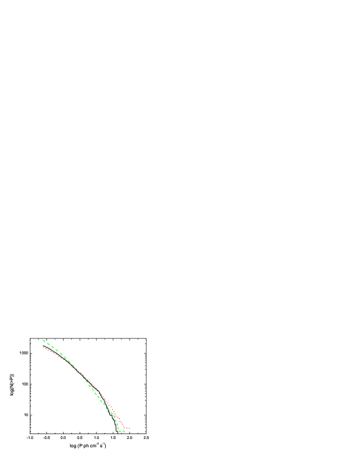
Figure 1: One-LF model fits to BATSE $\log N-\log P$ distribution. The solid line (black) denotes the observed BATSE $\log N-\log P$ distribution in each pane. From left to right (a-c), we have the models from G04 (G04 (green, dash); G04(2),(red, dotted)) G05 (P&M (green,dash); RR(red, dotted), and G07 with the largest $L_{min}$. The first two models (G04, G05) can roughly reproduce the observation, while the last model (G07) is ruled out by the data. The observed BATSE distribution is the solid black curve in all panes.

The simulated distributions of $L$, $z$, and $L-z$ in a two dimensional plane are shown in Fig. 2-4 along with the observational results. Without considering the LL-GRBs, the models of Guetta et al. (2004) can roughly produce the observed 1-dimensional $L$ and $z$ distributions. The model of Guetta & Della Valle (2007), however, causes a severe overproduction in bursts of luminosities $\sim 10^{48}-10^{50}\rm erg~{}s^{-1}$ at low redshifts and fails to reproduce bursts with z$>\sim$3 for the largest lower-luminosity cutoff of $5\times 10^{49}\rm erg~{}s^{-1}$ (see also Liang et al. 2007). The two-dimensional analysis, shown in Fig. 4, demonstrates this overproduction and makes note of the deficiency of bursts above $\sim 10^{52}~{}\rm erg~{}s^{-1}$ in all models. When LL-GRBs are considered, the models of Guetta et al. (2004) are insufficient since they predict a $\rho_{0}$ that is too low to account for the observed LL-GRBs. While the modified model by Guetta & Della Valle (2007) can accommodate a sufficiently low low-luminosity cutoff of $0.1L_{980425}$, the steep slope and low cutoff cause a large deviation from the observed $\log N-\log P$ distribution as discussed above.

3.2 Broken Power Law Model

A single power law LF model encounters great difficulty in simultaneously reproducing the observed HL/LL-GRB populations and the BATSE $\log N-\log P$ distributions. Therefore, we try the broken power law LF model (12), also discussed by Guetta et al. (2004,2005). The results of which are also shown in Figs. 1-4. The BPL model of G04 provides a distribution that peaks at around $z\sim$ 1, matching observations, as well as producing a similar number of bursts all around. As the parameters of the BPL are shifted for G05, the peak remains similar although the distribution becomes narrower. Apparently, these results are similar to that of the simple power law model and cannot explain both HL- and LL- GRBs and the $\log N-\log P$ distributions.

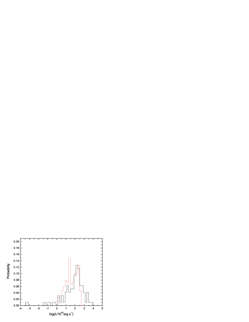
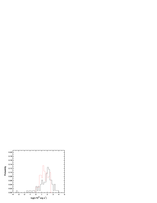
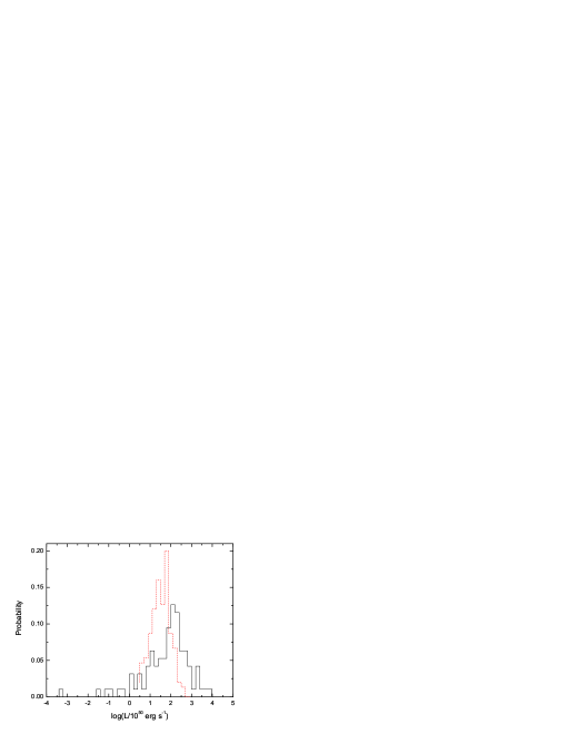
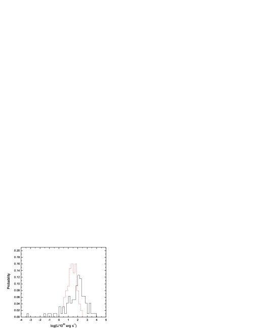
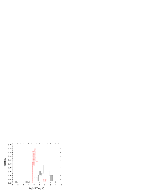
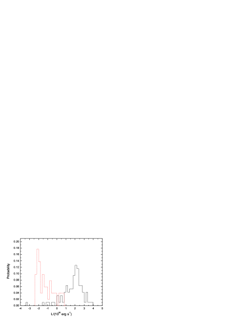
Figure 2: The 1-D luminosity distributions of various single-component LF models. The dashed curves (red) are the simulated results, while the solid curves (black) are the observed results for the redshift-known sample. Model parameters can be found in Table 1. The LF forms are, from left to right, G04, G04(2), G05 (P&M), G05 (RR), G07, G07(2).

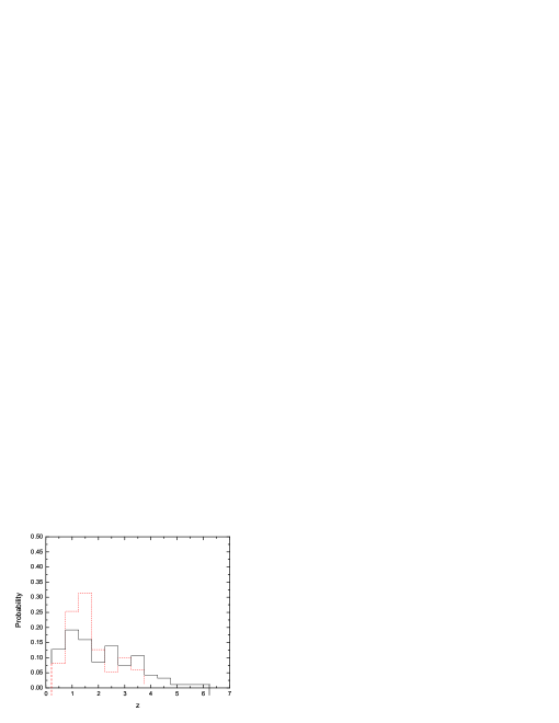
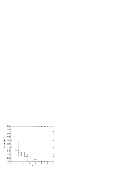
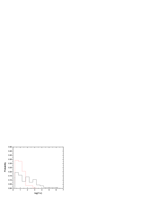
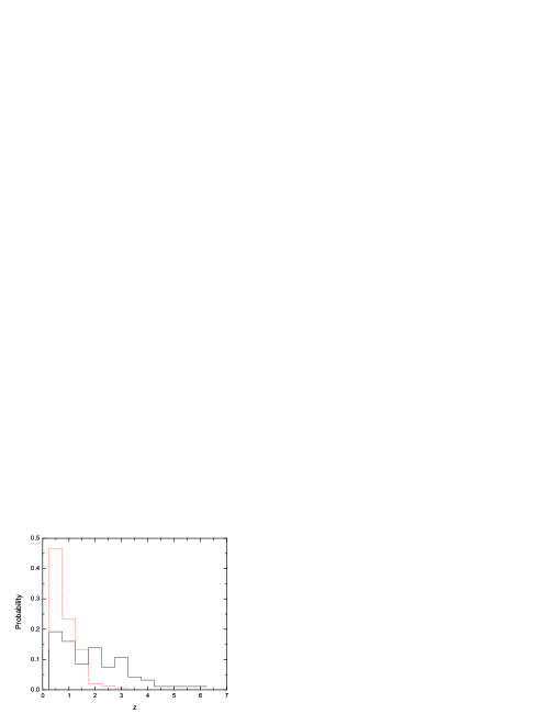
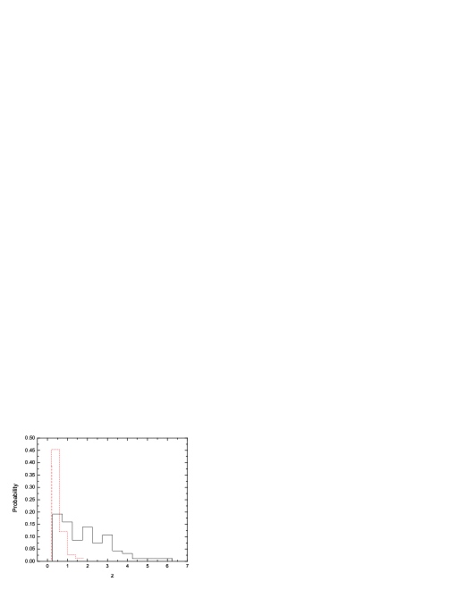
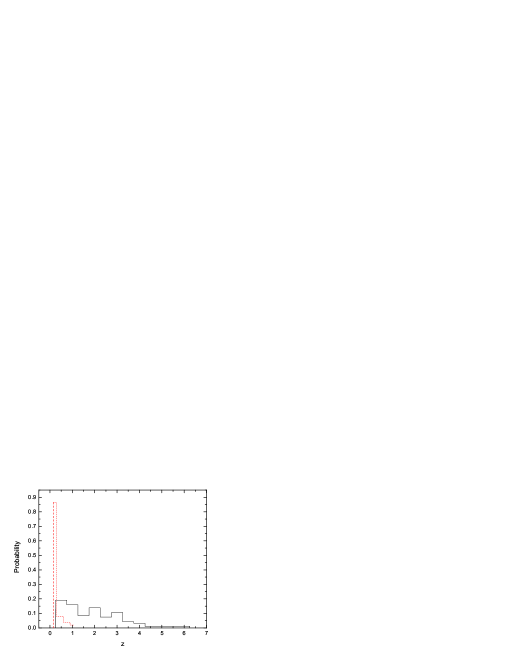
Figure 3: The 1-D redshift distributions of various single-component LF models. The dashed curves (red) indicate simulated results, while the solid curves (black) indicate the observed results for the redshift-known sample. The LF forms are, from left to right, G04, G04(2), G05 (P&M), G05 (RR), G07, G07(2).

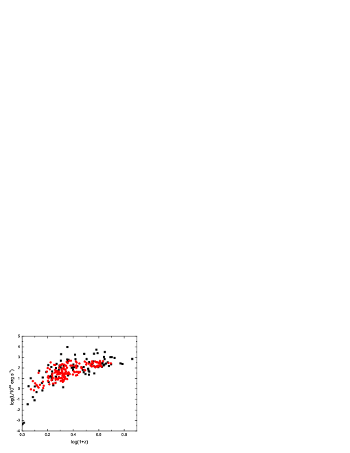
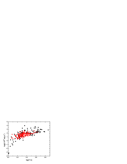
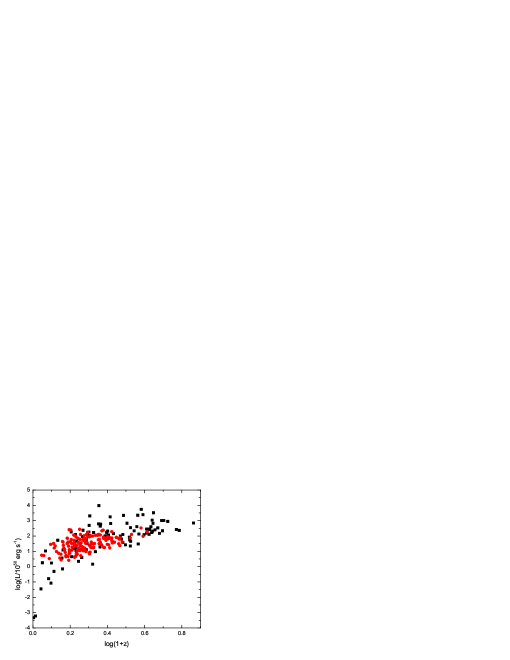
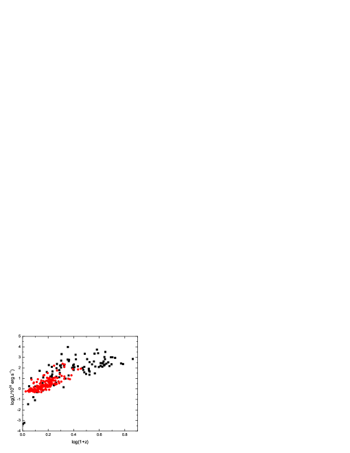
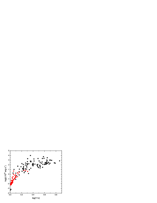
Figure 4: Two-dimensional luminosity-redshift distributions of various single-component PL models. The filled squares (black) are the observed redshift-known sample in the $z-L$ plane, while the filled circles (red) are the simulation results for models various models. The LF forms are, from left to right, G04, G04(2), G05 (P&M), G05 (RR), G07, and G07(2). None of these models are able to reproduce the observed distribution satisfactorily.

3.3 Combined Broken Power law Model: LL-GRBs as a Distinct GRB Population

Coward (2005) and Liang et al. (2007) proposed that LL-GRBs could be from a unique GRB population, characterized by low luminosity, less collimation, and high local rate compared to HL-GRBs. With the sensitivity threshold of BATSE and Swift BAT, these events are only detectable in a small volume, so that the number of detectable LL-GRBs could be low. With more sensitive detectors (e.g. JANUS, Roming et al. 2008; EXIST, Grindlay et al. 2006), one can probe into a larger volume which result in a larger number of detected LL-GRBs. To date only 2 LL-GRBs (GRBs 980425 and 060218) have been well-localized. The small number of LL-GRBs makes statistical testing of this population alone inaccurate. However, the high local LL-GRB rate inferred from the detection of GRBs 980425 and 060218 and the deficit of the observed GRBs with median luminosity ($10^{48}\sim 10^{49}\rm~{}erg~{}s^{-1}$) at redshift $0.1\sim 0.5$ place strong constraints on the luminosity function of this GRB population. It is unlikely that the lack of intermediate-redshift GRBs is the consequence of some selection effects. Since we are analyzing the intrinsic luminosities (rather than the observed fluxes), the deficit should not be related to an instrumental threshold effect, which requires that the LL-GRBs would diminish along with the intermediate luminosities GRBs. A redshift-dependent selection effect would require that there is a strong correlation between burst luminosity and redshift, which is not discovered from the data. We therefore conclude that the observations imply an intrinsic feature in the LF. Liang et al. (2007) suggested that the global GRB LF can be modeled with two components: a smoothed broken power law for each population. We elaborate this two-component model with our simulations.

The simulated GRBs cover a luminosity interval of $L=10^{45}-10^{55}\rm~{}erg~{}s^{-1}$ and a redshift interval of $z=0-10$. The values of luminosity and redshift assigned are subjected to the detector conditions described above, until a subset of 300 bursts (similar to the observed number of these types of bursts by Swift) is achieved. We then constrain the two-component LF parameters with the following procedure. First, we vary the parameters for the HL-GRB LF and compare with the observed 1-D $L-$ and $z-$ distributions as well as the 2-D $(L-z)$ distributions. Since the results are not sensitive to the value of $\alpha_{\rm 2,HL}$, we fix it at 2.5, and search for high-likelihood parameters in the $L_{b}-\alpha_{\rm 1,HL}$ space using K-S probability contours (Fig.5). This leads to high probability concentrations in a variety of spots. We then use the $\log N-\log P$ criterion to pin down the best parameter space.

Next, we constrain the LL-GRB component parameters using the 1-D and 2-D distributions as well as the relative ratio of the observed HL- and LL-GRBs. In order to address the number of simulated bursts that pass the threshold conditions, it is necessary to understand how each population was controlled. The number of LL bursts created was directly proportional to the number of HL- bursts created by the ratio of the local rates for each type of burst. The number of LL iterations was prescribed by

$$N_{LL}=N_{HL}\frac{\rho_{\rm 0,LL}}{\rho_{\rm 0,HL}}.$$ (15)

A change in either rate will result in different amounts of each type of burst created, which then affects the final distributions and observable number of bursts. It is necessary to note that the observable ratio of about 300:1 (HL:LL) bursts is for all triggered bursts, not just the redshift known subset. Therefore, the redshift-measurement probability condition (Eq. 14) need not be applied to the bursts since the purpose of this addition was to simulate the redshift measurement bias.

Analysis of the two component LF model shows promising results and constraints on the LF and local rate of both HL- and LL-bursts. It is found that the parameter set $(\alpha_{\rm 1,HL},\alpha_{\rm 2,HL},L_{b})=(0.425,2.5,5.2\times 10^{52}\rm~{}erg~{}s^{-1}$) gives a reasonable fit to both the $L-z$ constraints and the $\log N-\log P$ distribution, producing a strong peak in $L-z$ probability and fit to the $\log N-\log P$ distribution. For completeness, we also consider two other sets of parameters, $(\alpha_{\rm 1,HL},\alpha_{\rm 2,HL},L_{b})=(0.5,2.5,8\times 10^{52}\rm~{}erg~{}s^{-1}$) and ($0.475,2.5,7.2\times 10^{52}\rm~{}erg~{}s^{-1}$), which correspond to the second highest peak in $\alpha_{1}-L_{B}$ space, and a sample near the center of the maximum values of the contour. These parameter sets are the combination and result of the first three criteria for constraining the LF parameters, as mentioned in the introduction.

Moving on to the last criterion, the best fit parameters give number ratios of roughly 40:1 to 1000:1, depending on the assumed duration (and therefore instrument sensitivity) chosen for the set of bursts as well as the assumed values for the local event rates of both poulations. For $\rho_{0,LL}=100\rm~{}Gpc^{-3}~{}yr^{-1}$ (with $\rho_{\rm 0,HL}$ maintained at 1$\rm~{}Gpc^{-3}~{}yr^{-1}$), a duration (i.e. $t_{90}$) of 300s gives a ratio of 218:1 HL- to LL-bursts, in general agreement with observation. If the rate for these bursts is increased to 200 $\rm~{}Gpc^{-3}~{}yr^{-1}$ or 400 $\rm~{}Gpc^{-3}~{}yr^{-1}$, the durations that give reasonable results drop significantly, to 120 sec and 20 sec, respectively. This observable ratio is difficult to gauge, however, due to the few LL-GRBs that actually pass the threshold condition for instrument sensitivity and the fact that there could be a range of durations for individual bursts as well as uncertainty in the local rates. A change in both the duration, $\rho_{0,LL}$, and/or $\rho_{0,HL}$ will modify the set of parameters that will give the correct ratio, as shown above. For example, if one increases the duration from 120 sec to 500 sec and maintains a rate of 200 $\rm~{}Gpc^{-3}~{}yr^{-1}$, the number of LL-bursts detected increases about three-fold, significantly lowering the ratio. A similar change in ratio will occur when shifting the values of $\rho_{0}$. Small changes in the LF parameters of HL bursts (e.g. $L_{B}=6.85\times 10^{52}\rm~{}erg~{}s^{-1}$ modified to $9.85\times 10^{52}\rm~{}erg~{}s^{-1}$) do not significantly affect this ratio. More sensitive detectors (e.g. JANUS, Roming et al. 2008; EXIST, Grindley 2006) are crucial for the amassing of LL-burst data and will greatly assist determining typical timescales of these bursts, which affects the sensitivity of the detector, as well as further constrain the relative ratio and in generally improve statistics. The simulated LL-component should not significantly affect the bulk of the $L-z$ distributions and the $\log N-\log P$ distribution, but in the meantime gives rise to the desired LL-GRB events. Due to small number statistics, the LL-component parameters cannot be well constrained, especially for $\alpha_{\rm 1,LL}$. In any case, a set of parameters that can best reproduce the data can be obtained, which are summarized in Table 2.

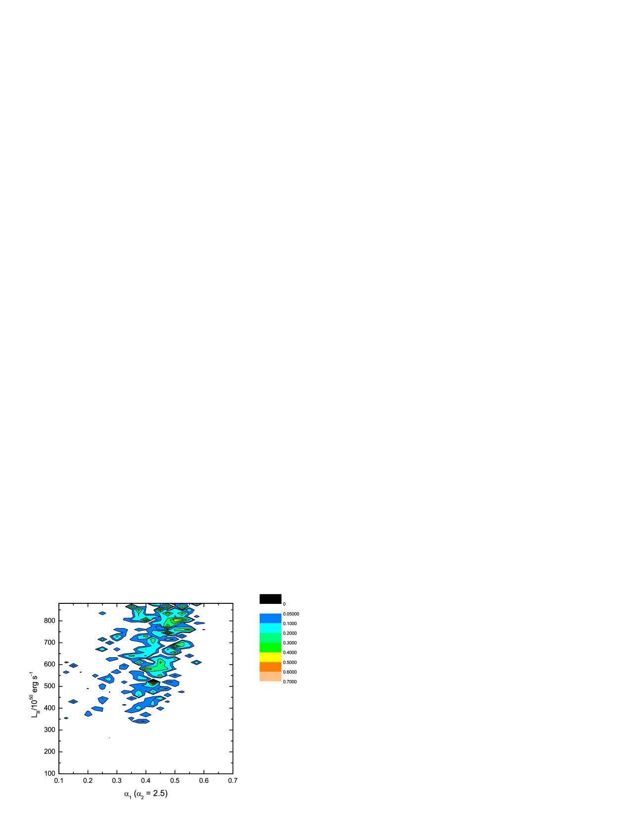
Figure 5: 2-D $p_{KS,t}$ contour as a function of $\alpha_{\rm 1,HL}$ and $L_{b}$ at $\alpha_{2}=2.5$.

Figures 6-9 graphically present the simulated results with the constrained parameters in Table 2 against the observational data, each set of graphs depicting a different constraint. Figure 6 shows the observed $\log N-\log P$ distributions superimposed with the simulated distributions for the two-component LF model. In addition to the BATSE sample (top curves), we also compare with the Swift/BAT sample (lower curves). The observed distributions seem to level off towards the low photon flux end. However, this is an effect created by the approach to the detection threshold of the particular instrument. The simulated results are not subjugated to such a cutoff, which serves as a prediction of the model for future observations by more sensitive detectors such as JANUS and EXIST. The simulated results are truncated at $0.01\rm~{}ph~{}cm^{-2}~{}s^{-1}$, roughly 20 times the BATSE sensitivity. The model also slightly overpredicts the number of bursts in the high luminosity end. However, since the number of very high-L GRBs is a small fraction of the total number of GRBs, this excess does not significantly worsen the fit to the data (see also Dai & Zhang 2005). The discrepancy might be interpreted as due to small number statistics. In general, the two component model reproduces the observed $\log N-\log P$ distribution much better than the other models presented in Fig.1.

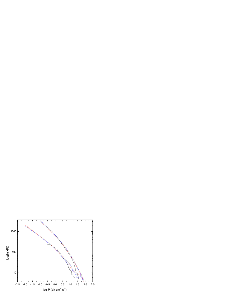
Figure 6: Two-component LF model fits to BATSE (top curves) and Swift/BAT (lower curves) $\log N-\log P$ distributions. The solid (black) curves are the observations, the dashed (blue) curves are the best fit parameters from the two-dimensional contour, the dotted (red) curves second peak in the probability distribution, and the dash-dot (gray) curves represent the middle parameters in the maximum of the $p_{KS,t}$ space (see table 3 for details).

Next we consider the 1- and 2-D $z$ and $L$ distributions whose results are summarized in Figs.(7-9). The simulated redshift distribution follows the observed distribution well through high $z$, except that the observations show a slight overproduction of bursts with $z>5$. This may be related to possible evolutionary effects or additional factors (e.g. metallicity) that determine the GRB rate (Kister et al. 2007; Daigne et al. 2007; Li 2007; Cen & Fang 2007), which we will fully address in a future work. The simulated 1-D luminosity distribution is also similar to the observed distribution, broadly peaking at $\sim 10^{52}\rm~{}erg~{}s^{-1}$. A slight deficit of bursts below $\sim 10^{50}\rm~{}erg~{}s^{-1}$ is seen in the data. This effect is most likely caused by the assumption of the probability for redshift measurement (Eq. 14), or perhaps an effect of a neglected redshift dependence (see discussion below). The 2-D $\log L-\log z$ distributions are detailed in Fig.9 and show that the simulated results generally match the band of observed bursts. There is a small underproduction of bursts of $10^{53}-10^{54}\rm~{}erg~{}s^{-1}$ at intermediate redshifts of z$\sim$3 as well as below $\sim 10^{50}\rm~{}erg~{}s^{-1}$. On the other hand, any attempt to increase the number of bursts in this luminosity range would skew the $\log N-\log P$ distribution at the high photon flux end. A possible cause may be that the fraction of bursts with redshift measurements in this $(L-z)$ range may be slightly higher due to the complicated selection effects which are not modeled. The two simulated LL-bursts are included in this graph, represented at the lower left hand corner very near the observed bursts. The number of HL-bursts plotted reflects the bias in measuring redshifts, namely that only $\sim$ 20 to 30 percent of HL-bursts have a measured redshift. Low-luminosity bursts are assumed to have a nearly 100 percent redshift detection rate thanks to their proximity.

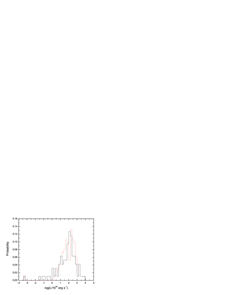
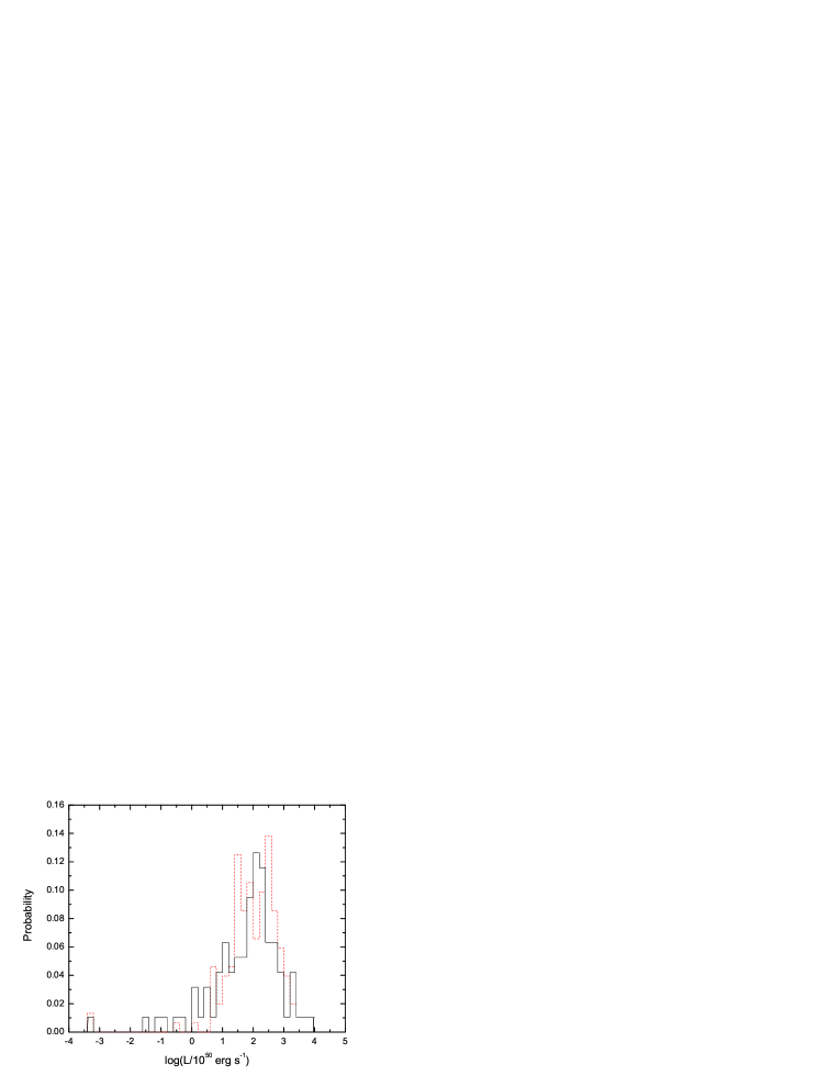
Figure 7: 1-D luminosity distribution of simulated GRBs (dashed) generated from the 2-component LF model compared to the observed GRBs (solid). The panels correspond to best, intermediate, and center K-S probability fits, respectively.

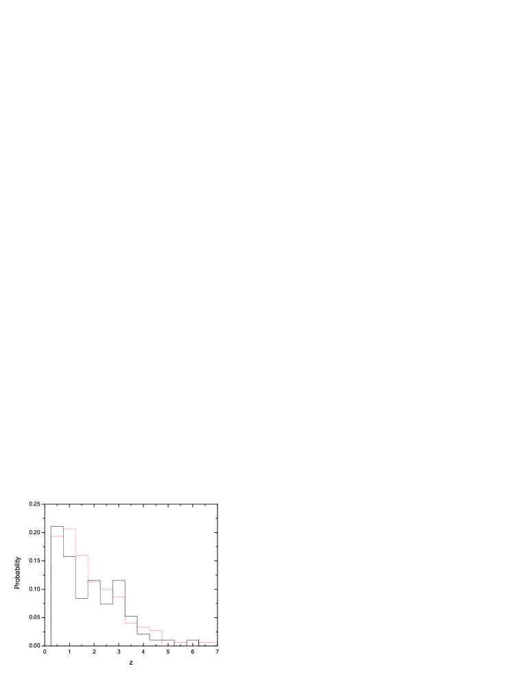
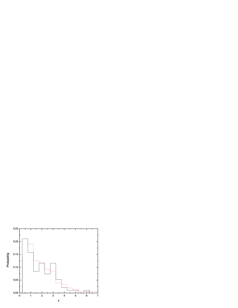
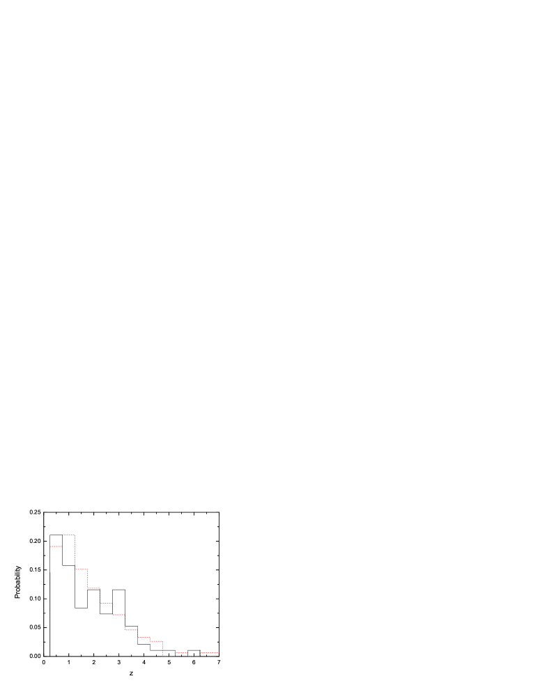
Figure 8: 1-D redshift distribution of simulated GRBs (dashed) generated from the 2-component LF model compared to the observed GRBs (solid). The panels correspond to best, intermediate, and center K-S probability fits, respectively.

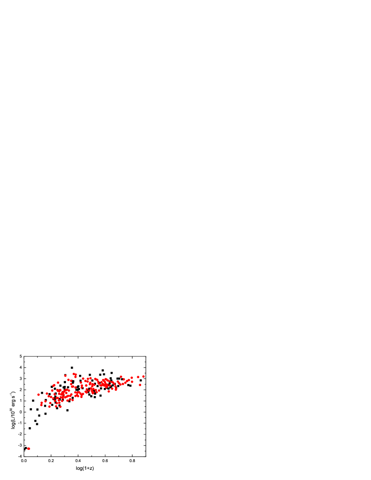
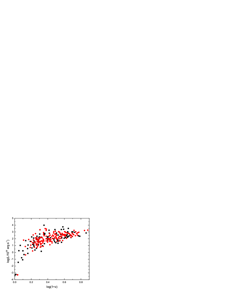
Figure 9: 2-D $(z-L)$ graph of simulated bursts from the 2-component LF model (red-circles) as compared to the observed GRBs (black, squares). The panels correspond to best, intermediate, and center K-S probability fits, respectively.

As mentioned above, intermediate LF parameters were used in producing Figs. 6-9. Finding more sophisticated functional forms of the trigger probability, simulating individual burst timescales, and/or adding terms that evolve with redshift will most likely increase the overlap of $p_{K-S,z}$ and $p_{K-S,L}$ which together constrain the LF parameters. Another factor that influences the K-S probability is the size of the sample of observed GRBs used in the analysis. As the Swift GRB sample continues to grow, and more bursts are observed with redshift measurements, the statistical possibilities for analysis will be also increased. To date, a total of 95 bursts have redshift measurements, 54 of those coming from Swift localizations.

4 Conclusions and Discussion

By utilizing Monte Carlo simulations and various test criteria we are able to further constrain the form and parameters of the LF of long GRBs. After confronting model results with various observational criteria, including 1-D and 2-D $L-z$ distributions of the redshift-known GRBs and the $\log N-\log P$ distributions of both CGRO/BATSE and Swift/BAT GRBs, we conclude that various one-component LF models discussed by previous authors (e.g. Guetta et al. 2004, 2005; Guetta & Della Valle 2007) are insufficient to account for all the data. As the luminosity function parameters are modified to accommodate for the observed LL-bursts, these models cause an overproduction of bursts at low and intermediate redshifts that is irreconcilable with the observed distributions. Although a PL or BPL would seem a simple and straight-forward solution to the LF problem, our reasoning and analysis imply that a two-component LF model (Liang et al. 2007, Coward 2005) is necessary. The latter model implies an event rate of local LL-GRBs of $\sim 100-400\rm~{}Gpc^{-3}~{}yr^{-1}$ at an $L_{B,LL}$ of $L\sim 10^{47}~{}{\rm erg~{}s^{-1}}$, which is much larger than that of HL-GRBs ($\sim 1\rm~{}Gpc^{-3}~{}yr^{-1}$). In addition, as mentioned in Liang et al. (2007), the functional form of the LL-bursts LF is quite uncertain, especially below the break luminosity. Most constraints are drawn from the more numerous HL observations, although important information about local rate and break luminosities for both distributions can be drawn simply from the number of LL-events detected within the time of Swift’s operation. Other effects that add difficulty to the analysis, but are addressed as fully as possible, include the inhomogeneity of the burst sample, redshift detection selection effects, and the relatively small sample size.

A recent development that may affect the local rate determination is the serendipitous discovery of a very low luminosity (peak luminosity $\sim 6.1\times 10^{43}~{}{\rm erg~{}s^{-1}}$) X-ray transient, XRF 080109, by Swift XRT (Soderberg et al. 2008). This event is associated with SN 2008D. Although it has been suggested that the X-ray emission may be related to shock breakout (Soderberg et al. 2008), the possibility that the X-ray emission is the jet emission from a very low luminosity X-ray flash has been suggested and cannot be ruled out from the data (Xu et al. 2008; Li 2008). In particular, the non-thermal spectrum of XRF 080109 makes it different from the thermal X-ray emission component discovered in XRF 060218, another shock-breakout emission candidate claimed in the literature (Campana et al. 2006). We therefore regard the origin of XRF 080109 inconclusive. If it is indeed a very low luminosity LL-GRB, its very high event rate (Soderberg et al. 2008; Xu et al. 2008) is consistent with the conclusion of this paper that LL-GRBs form a distinct new component in LF, and the event rate increases to even higher values towards low luminosities. This model also predicts the existence of X-ray flashes in the luminosity range of $10^{44}-10^{46}~{}{\rm erg~{}s^{-1}}$ that bridge XRF 080109 and XRF 060218.

The current LL-GRB sample is too small to address whether they follow the same empirical correlations as HL-GRBs, such as the lag-luminosity relation (Norris et al. 2005), variability - luminosity relation (Reichart et al. 2001), spectral peak energy - isotropic energy relation (Amati et al. 2002), etc. Apparent discrepancy exists for some (e.g. GRB 980425 as an outlier of the Amati-relation), but consistency exists for others (e.g. GRB 060218 satisfies the Amati and lag - luminosity relations, Liang et al. 2006; Amati 2006). On the other hand, these correlations are closely related to the radiation physics, which is not directly related to the central engine and progenitor of the bursts. The GRB fireball picture is very generic. Bursts with different types of progenitors may share the same emission physics and hence, similar empirical correlations. More data are needed to draw firmer conclusions in this direction.

In the analysis above we show that this 2-component LF model can interpret observations from both Swift and CGRO/BATSE in various criteria. Although some accommodations have been made to find common ground within all tests employed, these criteria shed light on the luminosity function problem and imply that a two-component LF is necessary. Various effects that are not considered in this work may further affect the luminosity and redshift distribution of the observed bursts. Changes to the form of the star formation rate appear often in the literature and are essential to the basic assumptions of long GRBs as being associated with the death of massive stars. Monte Carlo Simulations provide a useful tool for probing this effect, either as different functional forms of the SFR (Porciani and Madau 2001; Rowan-Robinson 1999; Hopkins and Beacom 2006) or deviations and evolutions with redshift (Kistler et al. 2007). Other effects that might affect the distributions include an evolution of the luminosity function with redshift (Lloyd-Ronning et al. 2002) or a dependence on cosmic metallicity (Li, 2007). These processes might provide solutions to the deficit of simulated bursts at high-luminosity and high-redshift, since most of these effects produce a larger rate of bursts at high redshift. Consequently, this redshift dependence does not affect the nearby LL-population. Understanding how and to what extent each of these processes affects the luminosity and redshift distributions is a necessary next step in the constraints of the luminosity function of GRBs, and we plan to explore them in full in a future work.

Single Component Luminosity Function Models
Model	Typea	$\alpha^{b}$	$\beta^{c}$	L${}_{B}^{d}$	L${}_{1}^{e}$	L${}_{2}^{f}$	$\rho_{0}$	$p_{KS,z}$	$p_{KS,L}$	$p_{KS,t}$
G04	SPL	-0.7	-	-	0.5	500	1.1	$0.00234$	0.00403	$9.4\times 10^{-6}$
G04 (2)	BPL	-0.1	-0.7	0.5	0.005	500	10	0.00018	0.00022	$3.96\times 10^{-8}$
G05 (P&M)k	BPL	-0.1	-2.0	71	71$/\Delta_{1}^{h}$	71$\Delta_{2}$	0.1	$1.23\times 10^{-9}$	$1.95\times 10^{-7}$	$2.4\times 10^{-14}$
G05 (RR)	BPL	-0.1	-2.0	71	71$/\Delta_{1}$	71$\Delta_{2}$	0.1	$8.1\times 10^{-12}$	$2.6\times 10^{-9}$	$2.1\times 10^{-20}$
G07	SPL	-1.6	-	-	0.5	500	1.1	$1.14\times 10^{-24}$	$2.24\times 10^{-19}$	$2.6\times 10^{-43}$
G07 (2)	SPL	-1.6	-	-	0.005	500	200	N/A	N/A	N/A
G07 (3)	SPL	-1.6	-	-	5$\times 10^{-4}$	500	200-1800j	N/A	N/A	N/A

Notes: a) SPL = simple power law, BPL = broken power law b) power law index c) For BPL models, power law index after the break luminosity d) break luminosity for broken power law e) lower luminosity cutoff in units of $10^{50}~{}\rm erg~{}s^{-1}$ f) high luminosity cutoff in units of $10^{50}~{}\rm erg~{}s^{-1}$ g) local GRB rate in units of Gpc^-3 yr${-1}$ h) $\Delta_{1}=30,\Delta_{2}=10$, See Guetta et al. (2005), j) Estimation from BATSE data, corrected to 110-1200 Gpc^-3 yr${-1}$ for BAT constraints (See Guetta 2007) k) Star forming rate model, Porciani and Madau (P&M) or Rowan-Robinson (RR).

Two Component Luminosity Function Model Parameters
$\alpha_{1}^{LL}$	$\alpha_{2}^{LL}$	L${}_{B}^{LL}$)a	$\rho_{0}^{LL}$b	$\alpha_{1}^{HL}$	$\alpha_{2}^{HL}$	L${}_{B}^{HL}$	$\rho_{0}^{HL}$	pKS,tc
0.0	3.5	$10^{47}$	100	0.425	2.5	$5.2\times 10^{52}$	1	$0.69$
0.0	3.5	$10^{47}$	100	0.5	2.5	$8.1\times 10^{52}$	1	0.474
0.0	3.5	$10^{47}$	100	0.45	2.5	$7.5\times 10^{52}$	1	0.167

Notes: a) $\rm erg~{}s^{-1}$ b) $\rm Gpc^{-3}~{}yr^{-1}$ c) Total K-S probability, $p_{KS,t}=p_{KS,L}\times p_{KS,z}$

Observed Gamma-Ray Bursts Data
GRB ID	$z$	$\log(L/{\rm erg~{}s^{-1}})$ a	Reference
970228	0.695	51.24	1
970508	0.835	51.16	2,3
970828	0.9578	51.52	4
971214	3.42	52.83	5
980326	1.00	52.03	6
980613	1.096	50.16	7
980703	0.966	52.21	8
990123	1.6	53.25	9
990506	1.3	52.63	10
990510	1.619	52.81	11
990705	0.842	51.97	12
990712	0.434	50.56	13
991208	0.706	51.39	14
991216	1.02	53.31	15
000301C	2.03	52.10	16
000418	1.118	52.22	17
000926	2.066	53.34	18
010921	0.45	51.08	19
011121	0.360	51.72	20
011211	2.14	51.42	21
020405	0.69	52.09	22
020531	1.00	52.25	23
020813	1.25	52.79	24
020903	0.25	48.92	25
021004	2.3	51.34	26
021211	1.006	52.69	27,28
030226	1.98	51.80	29, 30
030323	3.372	53.03	31
030328	1.52	52.31	32,33,34
030329	0.168	51.02	35
030429	2.65	53.35	36
040701	0.2146	49.21	37
040924	0.859	52.37	38
041006	0.716	51.66	39
050126	1.29	51.28	40
050315	1.949	52.00	41
050318	1.44	52.01	42
050319	3.24	52.41	43
050401	2.9	53.39	44
050416	0.6535	51.17	45
050505	4.3	52.95	46
050525	0.606	52.27	47
050603	2.821	53.74	48
050724	0.258	50.23	49
050730	3.97	52.34	50,51
050802	1.71	52.14	52
050820	2.61	52.61	53
050824	0.83	50.59	54

Table 3 continued
GRB ID	$z$	$\log(L/{\rm~{}erg~{}s^{-1}})$	Reference
050904	6.29	52.85	55
050908	3.344	52.22	56,57
051016B	0.9364	51.10	58
051109	2.346	52.54	59
051111	1.55	52.07	60
051221	0.5465	51.61	61
051227	0.714	50.86	62
060115	3.53	52.40	63
060124	2.296	51.91	64
060206	4.04998	53.01	65
060210	3.91	53.01	66
060614	0.125	50.25	67
980425	0.0085	46.67	68
060218	0.0331	46.78	69
031203	0.105	48.55	70
050826	0.297	49.69	71
050922C	2.199, 2.198	52.83	72, 104
060418	41.489	52.24	73,74
060502	1.51	51.80	75
060510B	4.9	52.43	76
060512	0.4428	49.85	77
060522	5.11	52.37	78
060526	3.21, 3.221	52.46	79, 104
060604	2.68	51.48	80
060605	3.78	52.18	81
060607	3.082	52.46	82
060707	3.425	52.19	83
060714	2.71, 2.711	52.13	84, 104
060904B	0.703	51.05	85
060906	3.686	52.53	86
060912	0.937	51.79	87, 105
060926	3.208	52.11	88
061004	0.3	52.60	106
061007	1.262	54.01	90
061110	0.757	50.35	91
061110B	3.44	53.52	92
061121	1.314	52.73	93
061222B	3.4	52.32	94
070110	2.352	51.64	95
070208	1.165	50.97	96
070306	1.497	52.01	97
070318	0.84	51.13	98
070411	2.954	52.08	99
070506	2.31	51.7661	100
070529	2.4996	52.28	101
070611	2.04	51.56	102
070612	0.617	50.64	103

References: 1) Djorgovski, S. G., et al., 1997, GCN 289 2) Bloom, J. S., et al., 1997, GNC3 30 3) Zharikov, S.V., et al., 1997, GCN3 31 4) Djorgovski, S. G., et al., 2001b, arXiv:astro-ph/0107539v1 5) Hogg, D. W., Turner, E. L., 1998, GCN 150 6) Fruchter A., et al., 2001a, GCN 1029 7) Djorgovski, S. G., et al., 1999, GCN 189 8) Djorgovski, S. G., et al., 1998 GCN 137 9) Gal, R. R., et al., 1999, GCN 213 10) Bloom, J. S., et al., 2001, arXiv:astro-ph/0102371v1 11) Vreeswijk, P. M., et al., 1999a, GCN 324 12) Le Floc’h et al. 2002, ApJ, 581, L81 13) Galama, T. J., et al., 1999 GCN 388 14) Dodonov, S. N., et al., 1999, GCN 475 15) Vreeswijk, P. M., et al., 1999b GCN 496 16) Castro, S. M., et al., 2000, GCN 605 17) Bloom, J. S., et al., 2000, GCN 661 18) Fynbo, J. P. U., et al, 2000, GCN 807 19) Djorgovski, S. G., et al., 2001a, GCN 1108 20) Infante, L., et al., 2001, GCN 1152 21) Fruchter, A., et al., 2001b, GCN 1200 22) Masseti, N., et al., 2002, GCN 1330 23) Kulkarni, S. R., et al., 2002, GCN 1428 24) Price, P. A., et al, 2002, GCN 1475 25) Soderberg, A. M., et al., 2002, GCN 1554 26) Chornock, R., et al., 2002, GCN 1605 27) Vreeswijk, P., et al., 2003a, GCN 1785 28) Della Valle, M., et al., 2003, GCN 1809 29) Greiner, J., et al., 2003a, GCN 1886 30) Price, P. A., et al., 2003, GCN 1889 31) Vreeswijk, P., et al., 2003b, GCN 1953 32) Martini, P., et al., 2003, GCN 1980 33) Rol, E., et al., 2003, GCN 1981 34) Maiorano, E., et al., 2006, arXiv:astro-ph/0601293v1 35) Greiner, J., et al., 2003b, GCN 2020 36) Weidinger, M., et al., 2003, GCN 2196 37) Kelson, D. D., 2004, GCN 2627 38) Wiersema, K., et al., 2004, GCN 2800 39) Price, P. A., et al., 2004, GCN 2791 40) Berger, E., et al., 2005b, GCN 3088 41) Kelson, D., Berger, E., 2005, GCN 3101 42) Berger, E., Mulchaey, J., 2005, GCN 3122 43) Fynbo, J. P. U., et al., 2005a, GCN 3136 44) Fynbo, J. P. U., et al., 2005b, GCN 3176 45) Cenko, S. B., et al., 2005, GCN 3542 46) Berger, E., et al., 2005a, GCN 3368 47) Foley, R. J., et al., 2005a, GCN 3483 48) Berger, E., Becker, G., 2005, GCN 3520 49) Prochaska, J. X., et al., 2005a, GCN 3700 50) Chen, H. W., et al., 2005, GCN 3709 51) D Elia, V., et al., 2005, GCN 3746 52) Fynbo, J. P. U., et al., 2005c, GCN 3749 53) Prochaska, J. X., et al., 2005b, GCN 3833 54) Fynbo, J. P. U., et al., 2005d, GCN 3874 55) Kawai, N., et al., 2005, GCN 3938 56) Fugazza, D., et al., 2005, GCN 3948 57) Foley, R. J., et al., 2005b, GCN 3949 58) Soderberg, A. M., et al., 2005, GCN 4186 59) Quimby, R., et al., 2005, GCN 4221 60) Hill, G., et al., 2005, GCN 4255 61) Berger, E., Soderberg, A. M., 2005, GCN 4384 62) Foley, J. R., et al., 2005c, GCN 4409 63) Piranomonte, S., et al., 2006, GCN 4520 64) Cenko, S. B., et al., 2006a, GCN 4592 65) Prochaska, J. X., et al., 2006, GCN 4593 66) Cucchiara, A., et al., 2006a, GCN 4729 67) Price, P. A., et al., 2006a, GCN 5275 68) Holland, S., et al, 2000, GCN 704 69) Mirabal, N., Halpern, J. P., 2006, GCN 4792 70) Prochaska, J. X., et al., 2003, GCN 2482 71) Halpern, J. P., Mirabal, N., 2006, GCN 5982 72) Jakobsson, P., et al., 2005, GCN 4017 73) Vreeswijk, P., Jaunsen A., 2006, GCN 4974 74) Dupree, A. K., et al., 2006, GCN 4969 75) Cucchiara, A., et al., 2006b, GCN 5052 76) Price, P. A., 2006b, GCN 5104 77) Bloom, J. S., et al., 2006a, GCN 5217 78) Cenko, S. B., et al., 2006b, GCN 5155 79) Berger, E., Gladders, M., 2006, GCN 5170 80) Castro-Tirado, A., J., et al., 2006, GCN 5218 81) Still, M., et al., 2006, GCN 5226 82) Ledoux, C., et al., 2006, GCN 5237 83) Jakobsson, P., et al., 2006a, GCN 5298 84) Jakobsson, P., et al.., 2006b, GCN 5320 85) Fugazza, D., et al., 2006, GCN 5513 86) Vreeswijk, P., et al., 2006, GCN 5535 87) Jakobsson, P., et al., 2006c, GCN 5617 88) D Elia, V., et al., 2006, GCN 5637 89) Jakobsson, P., et al., 2006d, GCN 5698 90) Osip, D., et al., 2006, GCN 5715 91)Thoene, C. C., et al., 2006, GCN 5812 92) Fynbo, J. P. U., et al, 2006b, GCN 5809 93) Bloom, J. S., et al., 2006b, GCN 5826 94) Berger, E., 2006, GCN 5962 95) Jaunsen, A. O., et al., 2007a, GCN 6010 96) Cucchiara, A., et al., 2007, GCN 6083 97) Jaunsen, A. O., et al., 2007b, GCN 6202 98) Jaunsen, A., O., et al., 2007c, GCN 6216 99) Jakobsson, P., et al., 2007, GCN 6283 100) Thoene, C. C., et al., 2007a GCN, 6379 101) Berger, E., et al., 2007, GCN 6470 102) Thoene, C. C., et al., 2007b, GCN 6499 103) Cenko, S. B., et al., 2007, GCN 6556 104) Jakobsson, P. et al., 2006e, A&A, 460, L13 105) Levan, A. J., et al., 2007, MNRAS, 378, 1439 106) Jakobsson, et al., 2006f, GCN 5702

Notes: (a) The spectral parameters and observed fluences in BAT band are taken from Sakamoto et al. 2007. In order to correct the observed fluence to the $1-10^{4}$ keV band in the burst rest frame, we derive the $E_{p}$ of each bursts with the relation between $E_{p}$ and the spectral power-law index (Zhang et al. 2007; Sakamoto et al. 2007) in the BAT band and assume that $\Gamma_{1}=-1$ and $\Gamma_{2}=-2.3$ for all bursts.