Hydrodynamical adaptive mesh refinement simulations of turbulent flows - II. Cosmological simulations of galaxy clusters

Abstract

The development of turbulent gas flows in the intra-cluster medium and in the core of a galaxy cluster is studied by means of adaptive mesh refinement (AMR) cosmological simulations. A series of six runs was performed, employing identical simulation parameters but different criteria for triggering the mesh refinement. In particular, two different AMR strategies were followed, based on the regional variability of control variables of the flow and on the overdensity of subclumps, respectively. We show that both approaches, albeit with different results, are useful to get an improved resolution of the turbulent flow in the ICM. The vorticity is used as a diagnostic for turbulence, showing that the turbulent flow is not highly volume-filling but has a large area-covering factor, in agreement with previous theoretical expectations. The measured turbulent velocity in the cluster core is larger than $200\ \mathrm{km\ s^{-1}}$, and the level of turbulent pressure contribution to the cluster hydrostatic equilibrium is increased by using the improved AMR criteria.

1 Introduction

The potential importance of turbulence for the physics of galaxy clusters has been widely recognised in recent years (see the discussion below for details and references). The precise nature of turbulence in the intra-cluster medium (ICM), however, remains controversial. The relevant dimensionless parameter for the onset of turbulence is the Reynolds number $Re$:

$$Re=\frac{LV}{\nu}\,\,,$$ (1)

where $L$ is the integral scale of the flow instability, $V$ is the characteristic velocity at scale $L$, and $\nu$ is the kinematic viscosity of the fluid. For a fully turbulent flow, $Re\ga 1000$. In the framework of galaxy cluster physics, the uncertainty in $Re$ results mostly from the determination of $\nu$. In the unmagnetised case, the Braginskii formulation (Braginskii, 1965) for the viscosity is generally used, leading to the frequently reported estimate of $Re\sim 100$ (e.g. Sunyaev et al., 2003) in the ICM.

This assumption does not hold in a magnetised plasma. As known from theory (Spitzer, 1962), the presence of magnetic fields suppresses the transport coefficients below the unmagnetised value by a factor $f$ which depends on the tangled field structure. While highly uncertain, it is estimated in the range $10^{-2}$ – $1$ (Reynolds et al. 2005; see also Narayan & Medvedev 2001). An effectively suppressed ($f\sim 10^{-2}$) viscosity would lead to $Re\gg 1$ both in the cluster cores and in the hotter and less dense ICM (Jones, 2007). On the other hand, it has been claimed that a factor $f\ga 0.1$ is consistent with the observation of filaments in the Perseus cluster (Fabian et al., 2003b). Irrespective of a more precise knowledge of $\nu$, it appears that the flow in the ICM is, even with a conservative estimate, mildly turbulent.

The turbulent nature of the flow in the intra-cluster medium (ICM) could be directly confirmed with the help of high-resolution X-ray spectroscopy of emission line broadening (Sunyaev et al., 2003; Dolag et al., 2005; Brüggen et al., 2005a; Rebusco et al., 2008). The unfortunate flaw in the main instrument of the Suzaku satellite postponed this test to the near future. Nevertheless, other observational clues have been interpreted as evidence for the turbulent state of the ICM, such as the analysis of pressure maps of the Coma cluster (Schuecker et al., 2004), the lack of resonant scattering in the $6.7\ \mathrm{keV}$ He-like iron $\mathrm{K_{\alpha}}$ line in the Perseus cluster (Churazov et al., 2004), the broadening of the iron abundance profile in the core of Perseus (Rebusco et al., 2005) and other galaxy clusters (Rebusco et al., 2006), and the Faraday rotation maps of the Hydra cluster (Vogt & Enßlin, 2005; Enßlin & Vogt, 2006). In addition to the astrophysical problems mentioned above, an improved knowledge of turbulence in the ICM can shed light on the amplification of magnetic fields (Dolag et al., 2002; Brüggen et al., 2005b; Subramanian et al., 2006), non-thermal emission in clusters (Brunetti, 2004), and acceleration of cosmic rays (Miniati et al., 2001a, b; Brunetti & Lazarian, 2007). The role of turbulence has also been investigated as a source of heating in cooling cores, as described in the analytical model by Dennis & Chandran (2005), where both the dissipation of turbulent energy and the turbulent diffusion are taken into account (cf. also Kim & Narayan 2003; Fujita et al. 2004a, b). In this context, the turbulence driven by galaxy motions in the ICM has been studied e.g. by Bregman & David (1989) and Kim (2007).

From a theoretical point of view, the production of turbulence in galaxy clusters has been ascribed to two main mechanisms. This work does not address the outflow of active galactic nuclei (AGN), which inflate buoyant bubbles and eventually stir the ICM, but will be focused on turbulence produced during the hierarchical formation of cosmic structures.

Several numerical simulations of galaxy cluster formation show that episodes of active merging can produce turbulence in the ICM (Ricker, 1998; Norman & Bryan, 1999; Takizawa, 2000; Ricker & Sarazin, 2001; Dolag et al., 2005), with typical velocities of $300$ – $600\ \mathrm{km\ s^{-1}}$ and injection scales of $300$ – $500\ \mathrm{kpc}$. In their simulations, Dolag et al. (2005) use a low-viscosity version of the gadget-2 SPH implementation (Springel, 2005), which helps to better resolve turbulent flows. Agertz et al. (2007) showed that grid methods are more suitable than SPH in modelling dynamical instabilities.

Since the properties of grid-based methods with regard to modelling turbulence are substantially better understood than SPH, we intend to explore their capability in the context of cosmological simulations. These, in turn, rely strongly on adaptive mesh refinement (AMR) in order to follow the evolution of strongly clumped media. Using AMR for turbulent flows is a new and rapidly evolving field (Kritsuk et al., 2006, 2007; Schmidt et al., 2008) which we extend to cluster simulations in this work.

The importance of a proper definition of the criteria for triggering grid refinement in turbulent flows has been studied by Iapichino et al. (2008) (hereafter paper I) by testing novel AMR criteria designed for resolving turbulent flows, and applying them in a simplified subcluster merger scenario. In this paper, we extend this work to cosmological AMR simulations of galaxy clusters. In this framework, we investigate how the AMR criteria tested in paper I can be profitably (from a physical and computational point of view) used for resolving the flow in the ICM. In AMR simulations of structure formation, both the refinement of turbulent flows and the the identification of small subclumps with a relatively low overdensity (O’Shea et al., 2005b; Heitmann et al., 2007) may be equally important; the relative emphasis has to be determined on a case-by-case basis. Both aspects and the related refinement strategies will be addressed in this work.

We focus our analysis on one single galaxy cluster out of the several objects forming in the simulated computational volume. An extended study of turbulence should be based on average cluster properties, sampling several objects of different masses (cf. Dolag et al. 2005; Vazza et al. 2006). Such a study is beyond the scope of this work and is left for future analysis.

The paper is organised as follows: in Sec. 2, we present the setup of the cosmological simulations and the set of employed AMR criteria. We discuss some general properties of the simulated cluster and present a performance comparison of the simulations in Sec. 3. In Sec. 4, the results are shown together with comparisons between the different runs. The results are summarised and discussed in Sec. 5.

2 Details of the simulations

Our work is based on the analysis and comparison of several cosmological simulations. In this section, their setup and the different AMR criteria are presented. The simulations were performed using the AMR, grid-based hybrid (N-Body plus hydrodynamical) code enzo (O’Shea et al., 2005a). The differences between the runs and the most significant modifications to the original public source code are presented in Sec. 2.2.

2.1 Common features

We performed hydrodynamical simulations in a flat $\Lambda$CDM background cosmology with $\Omega_{\mathrm{m}}=0.3$, $\Omega_{\mathrm{b}}=0.04$, $h=0.7$, $\sigma_{8}=0.9$, and $n=1$. The simulations were started with the same initial conditions at redshift $z_{\mathrm{in}}=60$, using the Eisenstein & Hu (1999) transfer function, and evolved to $z=0$. Cooling physics, feedback and transport processes are neglected. An ideal equation of state was used for the gas, with $\gamma=5/3$.

The simulation box had a comoving size of $128\ \mathrm{Mpc}\ h^{-1}$. It was resolved with a root grid (AMR level $l=0$) of $128^{3}$ cells and $128^{3}$ N-Body particles. A static child grid ($l=1$) was nested inside the root grid with a size of $64\ \mathrm{Mpc}\ h^{-1}$, $128^{3}$ cells and $128^{3}$ N-Body particles. The mass of each of the particles in this grid was $9\times 10^{9}\ M_{\sun}\ h^{-1}$. Inside this grid, in a volume of $(38.4\ \mathrm{Mpc}\ h^{-1})^{3}$, grid refinement from level $l=2$ to $l=7$ was enabled according to the criteria prescribed in Sec. 2.2. The linear refinement factor $N$ was set to 2, allowing an effective resolution of $7.8\ \mathrm{kpc}\ h^{-1}$ at maximum refinement level.

The static and dynamically refined grids were nested around the place of formation of a galaxy cluster, identified in a previous low-resolution, DM-only simulation using the HOP algorithm (Eisenstein & Hut, 1998). This cluster had a virial mass $M_{\mathrm{vir}}=5.8\times 10^{14}\ M_{\sun}\ h^{-1}$ and a virial radius $R_{\mathrm{vir}}=1.35\ \mathrm{Mpc}\ h^{-1}$ to within 1.3% and 0.4%, respectively, for all simulations. At $z=60$, the dynamically refined part of the computational domain contained more than $99.5\%$ of the N-Body particles that were within a virial radius from the cluster centre at $z=0$.

2.2 AMR criteria and other features

An overview of the most relevant features of the performed cosmological simulations is presented in Table 1. These runs differ with respect to the AMR criteria that were used after $z=2$ (with the exception of run $F$). Test calculations using the new criteria starting at $z=60$ showed no significant differences.

Table 1: Summary of the cosmological simulations performed for this work. The first column reports the name of the run, the second the criteria used for the grid refinement from $z=2$ (discussed in the text). The third column contains the number of AMR grids at $z=0$. Besides the reference run $A$, the horizontal line divides the remaining simulations in two groups, as explained in the text.

Run	AMR criteria	$N_{\mathrm{grids}}$
$A$	OD	2612
$B$	OD + 1	3871
$C$	OD + 2	3882
$D$	OD + 1 + 2	5358
$E$	OD, super-Lagrangian	4100
$F$	OD, low threshold	5340
	from $z=60$

Until $z=2$, all the simulations were run with the customary refinement criteria based on the overdensity of baryons and DM. In both criteria, a cell is refined if

$$\rho_{\mathrm{i}}>f_{\mathrm{i}}\rho_{0}\Omega_{\mathrm{i}}N^{l}\,\,,$$ (2)

where $\rho_{0}=3H_{0}^{2}/8\pi G$ is the critical density. In the case of baryons, $\rho_{\mathrm{i}}=\rho_{\mathrm{b}}$ (baryon density) and $\Omega_{\mathrm{i}}=\Omega_{\mathrm{b}}$; in the DM case, $\rho_{\mathrm{i}}=\rho_{\mathrm{DM}}$ (DM density) and $\Omega_{\mathrm{i}}=\Omega_{\mathrm{DM}}$.

The overdensity factors $f_{i}$ for baryons and DM are crucial for the resolution of cosmic structures (O’Shea et al., 2005b). If they are set too high, the AMR may fail in identifying low overdensity peaks, resulting in a deficiency of low-mass halos. In our simulations, unless stated differently, we set $f_{\mathrm{b}}=f_{\mathrm{DM}}=4.0$. This is the same as O’Shea et al. (2005b) for DM, and smaller by a factor of 2 for baryons. This overdensity criterion for baryons and DM is shortly named “OD” in Table 1. In our reference run $A$, only this criterion is used, whereas in the other simulations it is either modified or used in combination with other criteria.

In Table 1, the additional simulations are subdivided into two groups, corresponding to two different methods for better refinement of the turbulent flow. In the first group (runs $B$, $C$ and $D$), we use the AMR criteria based on control variables of the flow (Schmidt et al., 2008) and already tested in simulations of a subcluster merger (see paper I). The criteria implement a regional threshold for triggering the refinement, based on the comparison of the cell value of the variable $q(\mn@boldsymbol{x},t)$ with the average and the standard deviation of $q$, calculated on a local grid patch:

$$q(\mn@boldsymbol{x},t)\geq\langle q\rangle_{i}(t)+\alpha\lambda_{i}(t)\,\,,$$ (3)

where $\lambda_{i}$ is the maximum between the average $\langle q\rangle$ and the standard deviation of $q$ in the grid patch $i$, and $\alpha$ is a free parameter. Similar to paper I, we tested the square of the vorticity $\omega^{2}$ ($\mn@boldsymbol{\omega}=\nabla\mn@boldsymbol{\times}\mn@boldsymbol{v}$) and the rate of compression (the negative time derivative of the divergence $d=\nabla\cdot\mn@boldsymbol{v}$) as alternative or combined control variables. They are labelled as AMR criteria “1” and “2” in Table 1, respectively. Preliminary tests showed that, in cosmological simulations, these new criteria are effective only when used together with the overdensity criterion. In run $B$, the criteria “OD” and “1”, with threshold $\alpha=6.5$, are used. The run $C$ has been set with criteria “OD” and “2”, $\alpha=6.0$. In run $D$ the refinement is triggered by “OD” and both “1” and “2”, with $\alpha_{1}=7.2$ and $\alpha_{2}=6.2$.

Resolving turbulence in AMR cosmological simulations involves an additional requirement to tracking and refining turbulent flows. Since turbulence is driven largely by cluster mergers, particular care has to be taken to properly refine low-mass subclusters. Numerical studies (O’Shea et al., 2005b; Heitmann et al., 2007) indicate that the smallest halos being captured by the code depend on the overdensity thresholds and root grid resolution, rather than on the number of AMR levels. The second group of simulations (runs $E$ and $F$) is devoted to explore the problem of structure resolution, and to compare this approach with the new AMR criteria used in runs $B$, $C$ and $D$.

Run $E$ has a super-Lagrangian correction to the overdensity thresholds defined in equation (2), i.e.:

$$\rho_{\mathrm{i}}>f_{\mathrm{i}}\rho_{0}\Omega_{\mathrm{i}}N^{l(1+\phi)}\,\,,$$ (4)

where $\phi=-0.2$. The thresholds for refinement are lower than in run $A$, especially for higher AMR levels (cf. Wise & Abel 2007).

The implementation of more effective AMR overdensity criteria from $z=2$, as in run $E$, could produce a spurious suppression of small subclumps if they are not resolved from their formation at high redshift. In order to investigate this effect on the ICM turbulent motions, we performed the run $F$ with the criterion “OD” and thresholds $f_{\mathrm{b}}=f_{\mathrm{DM}}=2.0$, a factor of two smaller than run $A$, using these AMR criteria from $z=60$.

3 General cluster properties and AMR performance

Figure 1: Spherically averaged, mass-weighted radial velocity at $z=0$ in the reference run $A$. The cluster centre, needed for this analysis, was determined by the HOP tool as the location of the local density peak, with a maximum disagreement of $52\ \mathrm{kpc}\ h^{-1}$ ($0.04\ R_{\mathrm{vir}}$) in the performed simulations. The analysis tool is part of the enzo release.

The simulated cluster is widely relaxed, as can be inferred from its smooth spherically averaged radial velocity profile (Fig. 1) and from the time evolution of its mass accretion which indicates a steady growth due to minor mergers and excludes recent major merger events. In principle, this might be considered a poor case for studying turbulent flows in the ICM because of the lack of violent motions driven by major merger shocks (Ricker & Sarazin, 2001; Mathis et al., 2005). Nevertheless, this cluster provides a useful test for the study of turbulent motions generated mostly by accretion of minor subclumps, thus isolating the role of this phase of turbulence production.

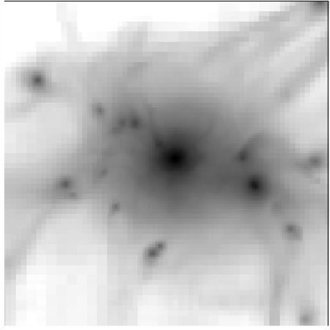
Figure 2: Projection on the $xy$ plane of a cube with a side of $8\ \mathrm{Mpc}\ h^{-1}(\approx 6\ R_{\mathrm{vir}})$, centred on the simulated galaxy cluster, and showing the baryon density at $z=0$ in a logarithmic gray-scale. The plot refers to run $A$, but it is not significantly different for other runs.

The morphology of the simulated cluster and its outskirts is shown in Fig. 2. Several accreting subclusters and the related gas stripping are visible, together with some filaments (e.g. in the upper right corner). The overall structure of the cluster does not change drastically in the performed simulations. However, interesting differences can be observed in the projected AMR structure (Fig. 3). The AMR grid follows the density (baryons and DM) distribution in run $A$ as well as in $E$ and $F$, where the effect of a lower AMR threshold results in a richer grid structure. As expected, the runs performed with the AMR criteria based on the regional variability of the control variables of the flow show that, in addition to the refinement on the density peaks, the grid structure is finer also in some locations which are correlated to the local velocity fluctuations and therefore to turbulent flows, rather than with the mass distribution. Since the analysis of the results will be largely focused on the cluster core (Sec. 4.3), Fig. 4 shows the projection of the AMR levels at the cluster centre at $z=0$. This part of the computational domain is generally highly resolved, though the grid coverage changes in the different runs.

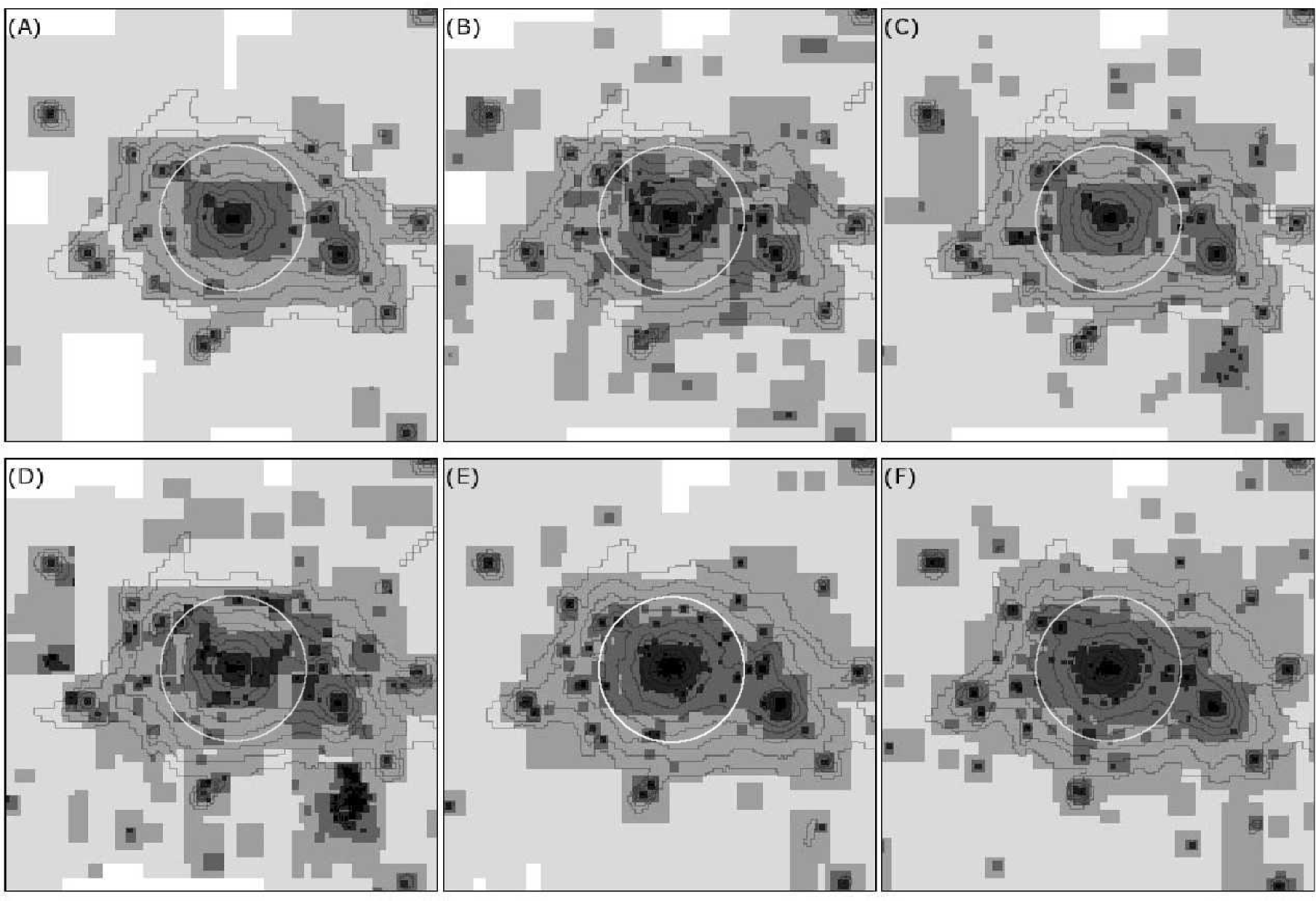
Figure 3: Projections similar to Fig. 2, but the projected AMR level is shown. The colour scale ranges from the AMR level 2 (white) to 7 (black like, for example, in the inner regions of the cluster). Baryon density contours are superimposed in gray. The radius of the white circles is $r=R_{\mathrm{vir}}$. The six panels refer to the performed runs, as indicated by the letter at the upper left corners.

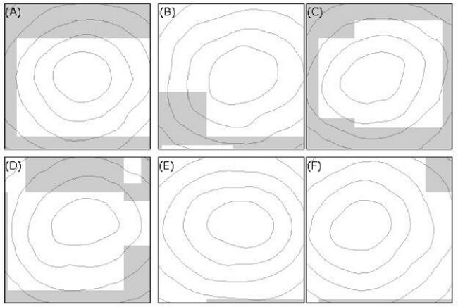
Figure 4: Projections similar to Fig. 3, but showing the projected AMR level in a zone with a side of $0.2\ R_{\mathrm{vir}}$, centred at the cluster core. The colour white corresponds to the AMR level $l=7$, and gray to $l=6$. Baryon density contours are superimposed in gray. The six panels refer to the performed runs, as indicated by the letter at the upper left corners.

From the point of view of grid complexity (and, consequently, of the required computational resources), our simulations form a rather homogeneous sample. In particular, the AMR thresholds of the simulations $B$–$F$ are tuned in a way to produce a number of AMR grids which do not greatly exceed $2\times N_{\mathrm{grids}}(A)$ (cf. Table 1).

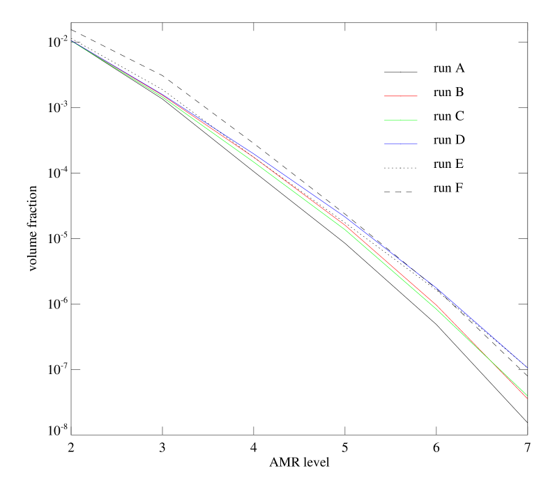
Figure 5: Occupation fraction of the AMR levels at $z=0$. The different lines refer to different simulations, according to the legend. The fraction is normalised to the whole computational domain. By construction of the setup, the occupation of level 1 is 0.125, and AMR from level 2 is allowed in a maximum volume of 0.027.

As an indicator for the efficiency of AMR, the volume occupation fraction as a function of the AMR level is shown in Fig. 5. The covering differences between the AMR criteria are more significant at high refinement levels (up to one order of magnitude at level 7). Regarding the efficiency of resolutions at higher levels, the simulations can be roughly grouped in three sets: the very resolved runs $D$, $E$ and $F$, the intermediate resolved $B$ and $C$, and the least resolved reference run $A$.

4 Properties of the turbulent flow in the ICM

4.1 Resolution of subcluster mergers

Before focusing on the features of the turbulent flow we present a qualitative account of the effectiveness of the new AMR criteria in refining substructures in the ICM. This analysis is directly relevant since we are concerned with turbulence driven by infalling subclumps.

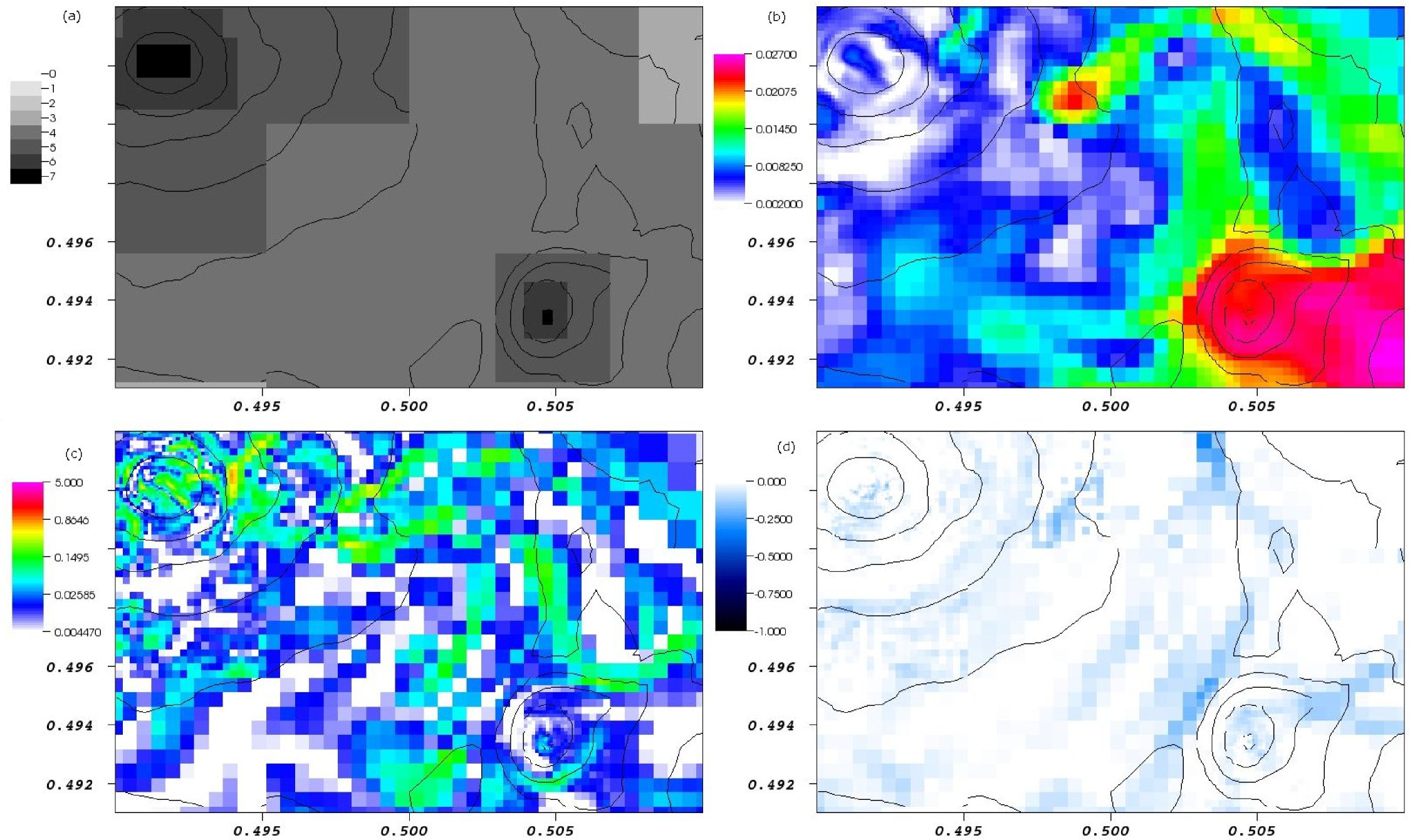
Figure 6: Slices of the $xz$ plane for run $A$ at $z=0$, showing a detail of the simulated cluster and its surroundings. The coordinates are given in code units ($1=128\ \mathrm{Mpc}\ h^{-1}$; $R_{\mathrm{vir}}\sim 0.01$). In all plots, baryon density contours are superimposed in black. (a): AMR levels. (b): gas velocity (corrected by the centre-of-mass velocity), in code units ($200\ \mathrm{km\ s^{-1}}\approx 0.003$). (c): Square of the vorticity modulus, in code units (cf. Sec. 4.2). (d): divergence of the flow, in code units.

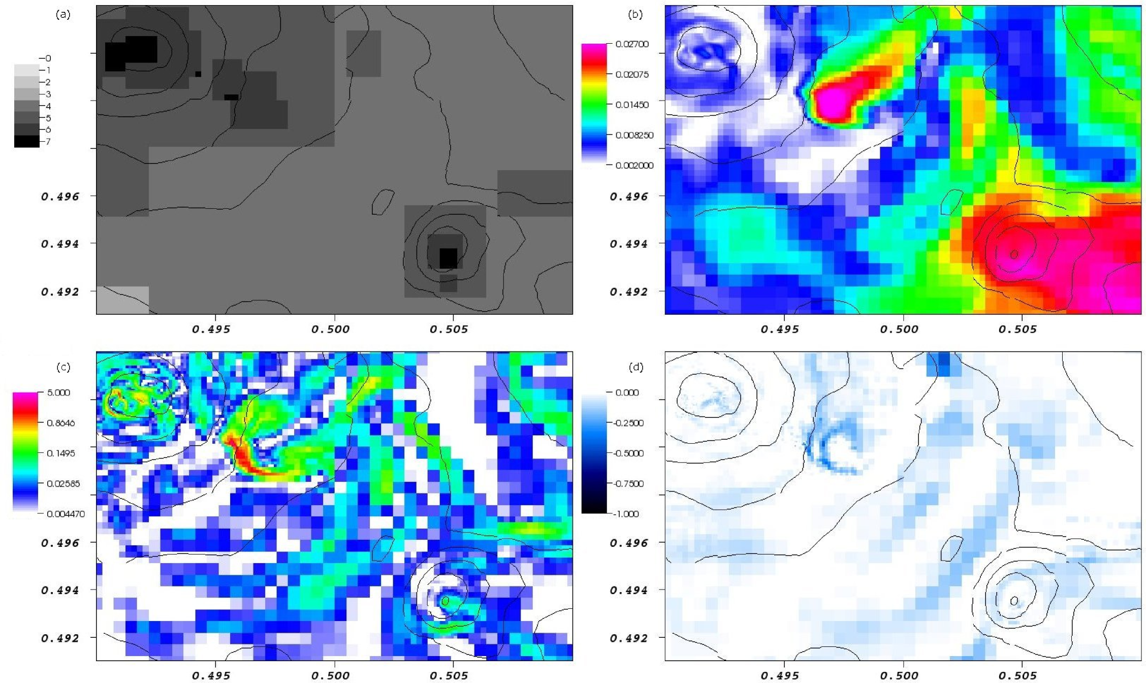
Figure 7: Same as Fig. 6, but for the run $B$.

For brevity, we limit most of this comparison to the runs $A$ and $B$. Figures 6 and 7 show some slices of the simulated cluster and its surroundings at $z=0$. We verified that the results do not depend on the choice of the slice plane. From the velocity slice (upper right panel) one can easily identify an infalling subcluster with a mass of about $2\times 10^{13}\ M_{\sun}\ h^{-1}$, at coordinates (0.505; 0.494), located just outside the virial radius, and a smaller (mass of the order of some $10^{12}\ M_{\sun}\ h^{-1}$) subclump at (0.498; 0.502) moving in the ICM. The projection of the motion of the first subcluster points roughly towards the cluster centre, while the second one moves to the left, parallel to the horizontal axis.

In Fig. 6, one can observe that the refinement level in the region of this subclump is $l=5$. Its signature in the vorticity plot is not very prominent. In the divergence slice, only negative values, i.e. converging flows, are shown, thus some of the visible structures are shocks. For example, a distinct feature (bow shock) is visible ahead of the larger subcluster, but it is less clear for the smaller one.

The application of the new AMR criteria affects the smaller merger more strongly because it is not highly refined in run $A$. Conversely, in run $B$ (Fig. 7) one can see that the front of the subclump is refined to $l=6$. The change is dramatic in the vorticity slice, where one can identify a large increase at the merger front and two parallel structures, likely to be caused by the lateral shearing flow. Also the signature in the divergence plot is clear and tracks the bow shock driven by the subclump.

The larger subcluster, which is relatively well refined in the reference run, does not profit further from the application of the new AMR criteria. However, the lateral shearing flow is clearly visible and in run $B$ a grid patch is added at (0.510, 0.496) because of the local peak in vorticity.

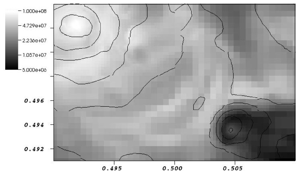
Figure 8: Slice of the $xz$ plane, at $z=0$, for run $B$ (same as the panels of Fig. 7), showing the gas temperature in $\mathrm{K}$, as indicated by the gray-scale. Baryon density contours are superimposed in black.

It is difficult to compare the evolution of these mergers with simulations of moving subclusters in a simplified setup (paper I and references therein). Even if the level of effective resolution is formally similar, the subclusters presented here have less details than in paper I because of their smaller size, and the background flow is far from homogeneous, in contrast with the artificial merging setup. Nevertheless, some gross features of the smaller subclump resemble the simplified setup, like the side distribution of the vorticity. With the use of the new AMR criteria, it is also easier to visualise the mergers in the temperature slice of run $B$ (Fig. 8), where they show the well known cold front morphology.

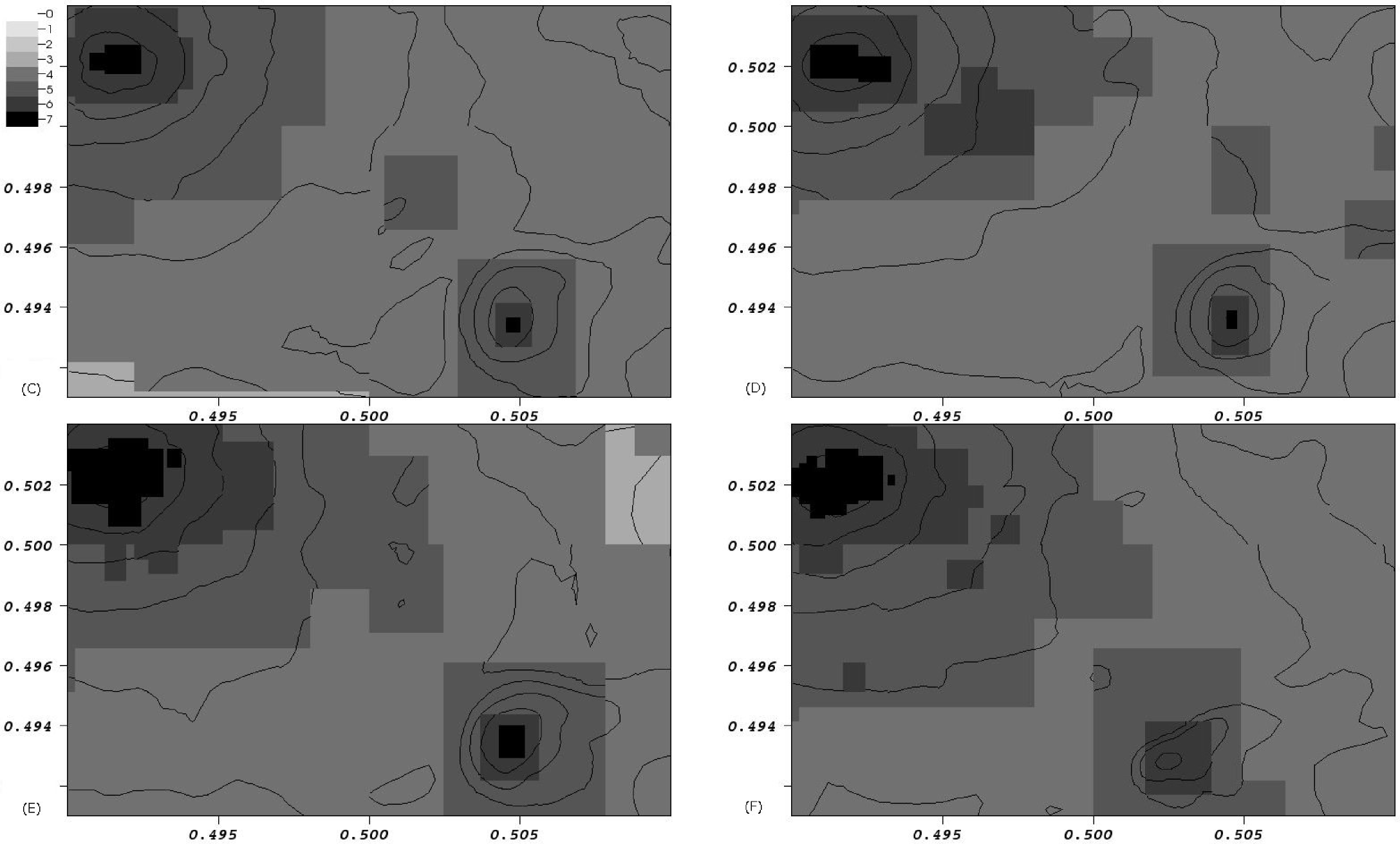
Figure 9: Slices of the AMR levels, on the $xz$ plane, at $z=0$, for the runs $C$–$F$ (same as the upper left panels of Figs. 6 and 7). The panels refer to the performed runs, as indicated by the letter at the lower left corners.

For completeness, Fig. 9 shows the slices of the AMR levels for the runs $C$–$F$. The position of the smaller subclump is resolved to $l=6$ only in run $D$, which implements the AMR based on the regional variability of $\omega$ like $B$, and in run $F$, which has a lower AMR density threshold. The run $C$ does not refine the subclump above $l=5$, but this is not necessarily an indication of an insufficient performance in refining turbulent flows. More accurate diagnostics of the resolution on velocity fluctuations will be introduced in the next sections.

4.2 Volume-filling and area-covering factors

Using analytical models, Subramanian et al. (2006) study the dynamics of turbulence generation in clusters during the infall of minor mergers. Under reasonable estimates for the merger rate and assuming simple models for the geometry of the turbulent subcluster wakes, those authors found that the volume simultaneously occupied by merger wakes (expressed by the volume-filling factor $f_{V}$ as a fraction of the ICM volume) is relatively small, but the projections of the wakes on the sky plane $f_{S}$ cover a large fraction of the cluster area.

Given a reasonable choice of the involved parameters, assuming a viscosity suppression factor $f\sim 0.2$ and requiring that the wake length is of the order of $2\ R_{\mathrm{vir}}$, Subramanian et al. (2006) report for a cluster mass of about $10^{15}\ M_{\sun}$ the indicative values

$$f_{V}\sim 0.25,\qquad f_{S}=O(1)$$

which depend strongly on $f$. According to those authors, a combination of a high area-covering factor and a relatively lower volume-filling factor can reconcile the observation of ordered filaments in Perseus with indications for turbulence in the ICM of that cluster. The idea that turbulence is not completely volume-filling in the ICM is, moreover, a further motivation to use AMR in this problem, saving computational resources (cf. Kritsuk et al. 2006).

In order to probe these features of the turbulent flow in the performed cosmological simulations, one needs to find a suitable way to track turbulence. Velocity fluctuations are one of the distinctive features of turbulence, therefore quantities related to the spatial derivatives of velocity can be used profitably for this aim. In analogy with paper I, the norm of the vorticity $|\mn@boldsymbol{\omega}|$ will be used to probe the velocity fluctuations at the length scale allowed by the spatial resolution, as a diagnostic for the resolved turbulent motions. The onset of eddy-like motions is closely related to the baroclinic generation of vorticity, expressed by taking the curl of both sides of the inviscid Euler equation:

$$\frac{\partial\mn@boldsymbol{\omega}}{\partial t}=\nabla\mn@boldsymbol{\times}(\mn@boldsymbol{v}\mn@boldsymbol{\times}\mn@boldsymbol{\omega})-\frac{\nabla p\mn@boldsymbol{\times}\nabla\rho}{\rho^{2}}$$ (5)

where $p$ is the pressure of the gas. The second term on the right-hand side is nonzero if the two gradients are not parallel, i.e. at curved shocks (Kang et al., 2007) and at the interface of infalling subclumps.

This analysis was restricted to a sphere including the innermost $0.5\ R_{\mathrm{vir}}$ of the cluster, at $z=0$. As a threshold for flagging a computational cell as “belonging to the turbulent flow”, we chose the mass-weighted average of the vorticity norm in run $A$ within the central sphere, $\langle|\mn@boldsymbol{\omega}|(A)\rangle$. The volume-filling factor $f_{V}$ is thus defined as the fraction of the analysis volume where $|\mn@boldsymbol{\omega}|>\langle|\mn@boldsymbol{\omega}|(A)\rangle$. If the vorticity is interpreted as the inverse of the eddy turnover time (Kang et al., 2007), the chosen threshold corresponds to a large number ($\sim 50$) of local eddy turnovers, assuring a conservative estimate of the extent of the turbulent regions.

The results of this analysis are summarised in Table 2. The vorticity is reported in enzo code units. Dimensionally, the vorticity is expressed as $[t^{-1}]$, and the time unit in enzo is $1/(4\pi G\Omega_{\mathrm{m}}\rho_{0}(1+z_{\mathrm{in}})^{3})^{1/2}$, with the meaning of the symbols introduced above.

Table 2: Results of the vorticity analysis. The first column reports the name of the run, the second the mass-weighted average of the vorticity norm $|\mn@boldsymbol{\omega}|$ in the sphere with radius $0.5\ R_{\mathrm{vir}}$. The maximum value of $|\mn@boldsymbol{\omega}|$ is listed in the third column, and the volume-filling factor is reported in the fourth. The vorticity data are expressed in code units.

Run	$\langle|\mn@boldsymbol{\omega}|\rangle$	$\max{(|\mn@boldsymbol{\omega}|)}$	Volume-filling
	(code units)	(code units)	factor
$A$	0.211	1.42	0.233
$B$	0.209	4.04	0.231
$C$	0.215	2.05	0.243
$D$	0.226	2.75	0.279
$E$	0.238	1.59	0.297
$F$	0.246	1.49	0.297

Interestingly, the volume-filling factor is not substantial and has a value somehow comparable with the theoretical expectations of Subramanian et al. (2006). Apart from the exact value of $f_{V}$, which theoretically depends on many parameters and, in our simulations, on the assumptions about the threshold of $|\mn@boldsymbol{\omega}|$, the turbulent flow does not appear very volume-filling ($f_{V}\la 0.3$ for all runs).

When the results of the performed runs are compared, the features of the vorticity are quite different in the two groups of simulations introduced in Sec. 2.2. In particular, in the first group (with the exception of run $D$, to be discussed) $\langle|\mn@boldsymbol{\omega}|\rangle$ and $f_{V}$ are not much larger than for run $A$, but $\max({|\mn@boldsymbol{\omega}|})$ is. In the second group the opposite occurs: $\langle|\mn@boldsymbol{\omega}|\rangle$ and $f_{V}$ are larger than run $A$, while $\max{(|\mn@boldsymbol{\omega}|)}$ does not vary substantially.

These results can be interpreted in terms of the difference between runs that mostly refine on the flow (first group) and those that refine on the substructures (second group). In the first case, especially for run $B$ that refines explicitly only on vorticity, the maximum resolved value of $|\mn@boldsymbol{\omega}|$ is larger, but it does not improve the overall efficiency in locally resolving the turbulent flow. In the latter group, conversely, the AMR does not focus on the turbulent flow, but the grid captures the overdense subclumps more efficiently, which increase $\langle|\mn@boldsymbol{\omega}|\rangle$ and $f_{V}$ by stirring the ICM.

It is known (Plewa & Müller, 2001) that some spurious vorticity is generated at the boundary of grids of different refinement levels. One could therefore conjecture that the runs with the largest number of grids are potentially affected by this problem. The large $f_{V}$ in the run $D$ might be partly due to this issue, because it has more grids than runs $B$ and $C$. Nevertheless, we can exclude that this effect dominates the presented results. Evidence supporting this statement is provided by run $E$, which has $N_{\mathrm{grids}}$ similar (to within 5%) to runs $B$ and $C$, but very distinct flow properties.

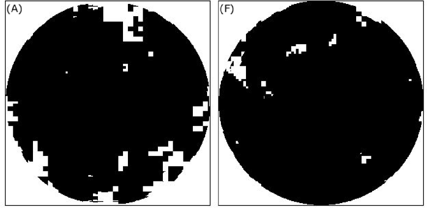
Figure 10: Projection of the analysis sphere onto the $xy$ plane, showing the area-covering factor $f_{S}$. In the black zones, $|\mn@boldsymbol{\omega}|>\langle|\mn@boldsymbol{\omega}|(A)\rangle$ along the line of sight. The two panels refer to the runs $A$ (left) and $F$ (right), as indicated by the letter at the upper left corners.

The area-covering factor resulting from these data can be visually inspected in Fig. 10, for the representative cases of runs $A$ and $F$. The turbulent flow, in agreement to Subramanian et al. (2006), has $f_{S}$ close to unity. As expected, the area-covering factor is larger in runs with a larger $f_{V}$.

4.3 Turbulent features: the ICM and the cluster core

The analysis of the geometry of the turbulent flow presented above is complementary to the knowledge of the magnitude of the turbulent velocity. From an operational point of view (cf. Dolag et al. 2005), the calculation of a root mean square (henceforth rms) velocity implies the definition of an average reference velocity, in order to distinguish between the bulk velocity flow and the velocity fluctuations.

In the case of spherically averaged radial profiles, the most natural choice is to use the average velocity $\langle v(r)\rangle$ in the spherical bin $r\pm\Delta r$. The mass-weighted rms baryon velocity is then defined as

$$v_{\mathrm{rms}}(r)=\sqrt{\frac{\sum_{i}m_{i}(v_{i}-\langle v(r)\rangle)^{2}}{\sum_{i}m_{i}}}\,\,,$$ (6)

where $m_{i}$ is the mass contained in the cell $i$, and the summation is performed over the cells belonging to the spherical shell of amplitude $r\pm\Delta r$.

Figure 11: Spherically averaged, mass-weighted radial profile of the rms baryon velocity at $z=0$ for the reference run $A$. The definition of the rms velocity is provided in the text.

The radial profile of $v_{\mathrm{rms}}$ for the reference run $A$ is shown in Fig. 11. The rms baryon velocity is a fraction of the virial velocity $\sigma_{\mathrm{vir}}=\sqrt{GM_{\mathrm{vir}}/2R_{\mathrm{vir}}}\approx 960\ \mathrm{km\ s^{-1}}$. This is similar to the results of Norman & Bryan (1999) and Dolag et al. (2005), though in the latter case the quantitative comparison is more difficult, because our cluster is outside the mass ranges which those authors explored.

The radial profile of $v_{\mathrm{rms}}$ at $r\ga 0.1\ R_{\mathrm{vir}}$ for the runs $B$–$F$ does not differ significantly from Fig. 11. This result could be considered a shortcoming of the adopted approach for the resolution of turbulent flows in the ICM, but can be easily explained by the properties of turbulence and the features of the performed AMR simulations. In fact, the volume filling factor of turbulence is not very large, so any quantitative change in $v_{\mathrm{rms}}$ is likely to be washed out when averaged on a spherical shell. Closely related to this point, the AMR thresholds imposed to avoid an excessive number of grids particularly affect the ICM where the volume of each spherical shell is increasingly larger.

In the small volume of the cluster core, where the level of refinement is relatively higher than in the ICM, the refinement strategies are more effective and the use of different AMR criteria introduces more relevant changes between the simulations. We notice that also in Dolag et al. (2005) (probably for reasons related to the turbulence filling factor), the region where turbulent motions are most important is localised in the inner $\approx 0.1\ R_{\mathrm{vir}}$. In the core region of the cluster, the analysis was not performed on radial profiles because this tool proved not to be robust for $r\la 0.07\ R_{\mathrm{vir}}$, probably because of sampling issues. In particular, the baryon rms velocity profile in the innermost part of the cluster is very sensitive to small displacements of the centre and to the calculation of $\langle v(r)\rangle$. Therefore, the mass-weighted averaged quantities within a sphere of radius $R=0.1\ R_{\mathrm{vir}}$, centred at the cluster centre, provide a more robust diagnostic for the resolution of turbulent flows in the cluster core.

Table 3: Mass-weighted values of some hydrodynamical quantities, calculated within a sphere with $R=0.1\ R_{\mathrm{vir}}$ centred at the cluster centre at $z=0$. For the different runs (first column), the table lists the rms baryon velocity $v_{\mathrm{rms}}$ (second column), the baryon density $\rho$ (third), the temperature $T$ (fourth), the ratio of turbulent to total pressure $P_{\mathrm{turb}}/P_{\mathrm{tot}}$ (fifth, defined in the text) and the entropy $S=T/\rho^{\gamma-1}$, with $\gamma=5/3$ (sixth).

Run	$v_{\mathrm{rms}}$	$\rho$	$T$	$P_{\mathrm{turb}}/P_{\mathrm{tot}}$	$S$ ($10^{5}\ \times$
	($\mathrm{km\ s^{-1}}$)	($10^{-26}\ \mathrm{g\ cm^{-3}}$)	($10^{7}\ \mathrm{K}$)	(%)	code units)
$A$	211	1.13	7.85	1.37	3.11
$B$	240	1.05	8.14	1.71	3.41
$C$	298	1.04	7.97	2.69	3.37
$D$	266	1.07	8.23	2.08	3.39
$E$	239	1.09	8.04	1.72	3.26
$F$	272	1.05	7.91	2.26	3.32

The results of the core analysis are summarised in Table 3. For the calculation of $v_{\mathrm{rms}}$, equation (6) was applied, where $\langle v(r)\rangle$ is the mean velocity in the analysis sphere. The rms velocity is the quantity that shows the largest variation between the reference run $A$ and runs $B$–$F$, with an increase of about 40% for run $C$. We notice that the highest value is predicted in a run belonging to the first group.

Among the first group, run $C$ seems more effective than run $B$. A possible reason is that the AMR implemented in run $B$ is not designed to refine explicitly on shocks (cf. Paper I), which are ubiquitous in the cluster medium (Miniati et al., 2000; Ryu et al., 2003; Kang et al., 2007). Despite of the larger number of grids, run $D$ has features which are comparable with runs $B$ and $C$, probably because of the larger thresholds used for its refinement criteria.

In the second group, run $F$ performs slightly better than run $E$. Comparing the density thresholds for refinement in these two runs (equations (4) and (2), respectively, with the appropriate parameters), one can see that the thresholds in run $E$ are smaller for $l>5$, namely in most of the cluster core. Therefore, the better performance of run $F$ in the core is not due to a more intensive, local use of AMR, but is likely to be caused by the more accurate tracking of subclumps along the whole cluster evolution.

Other variables are also listed in Table 3. For density, temperature and entropy the variations introduced by the use of different AMR criteria are smaller than in the case of $v_{\mathrm{rms}}$ (about 10%, at most, for density and entropy, and 5% for temperature).

The ratio of turbulent to total pressure (fifth column in Table 3) is defined as:

$$\frac{P_{\mathrm{turb}}}{P_{\mathrm{tot}}}=\frac{v_{\mathrm{rms}}^{2}/3}{kT/(\mu m_{\mathrm{p}})+v_{\mathrm{rms}}^{2}/3}\,\,,$$ (7)

where $k$ is the Boltzmann constant, $\mu=0.6$ is the mean molecular weight in a.m.u., $m_{\mathrm{p}}$ is the proton mass, and $T$ is the mass-weighted temperature (fourth column in Table 3).

The contribution of $P_{\mathrm{turb}}$ to the total pressure in the cluster centre is marginal, but we notice that it is increased (in case of run $C$, almost doubled) in the new runs. The increase of $P_{\mathrm{turb}}$ is consistent with the decrease in density: the turbulent motions introduce an additional term to the pressure equilibrium, which is balanced by a smaller baryonic pressure and a smaller central density.

An increase in temperature and entropy with respect to run $A$ are also observed. The moderate increase in entropy is similar to what is observed in Dolag et al. (2005), when the low-viscosity version of SPH is used. In that work, the increase was ascribed either to a better shock modelling or to a more efficient gas mixing. Both features can be retrieved in our AMR simulations $B$–$F$, at some degree, so we agree with this interpretation.

The trend in temperature is compatible with the enhanced dissipation of kinetic to internal energy, although the increase is not closely related with the value of $v_{\mathrm{rms}}$. We verified that the increase in the internal energy in the new runs is comparable, by order of magnitude, to the increase of the energy dissipation $\Delta E=(\Delta v)^{3}\tau/2\delta$, where $\Delta v$ is the increase of $v_{\mathrm{rms}}$, $\delta$ is the effective spatial resolution and $\tau$ is a time on the Gyr-scale.

Figure 12: Spherically averaged, mass-weighted radial profile of the ratio of turbulent to total pressure (defined in the text), at $z=0$, for the reference run $A$.

Figure 12 displays the radial profile of the turbulent to total pressure outside the cluster core, for the run $A$. Equation 7 was used for the computation of $P_{\mathrm{turb}}/P_{\mathrm{tot}}(r)$, with $v_{\mathrm{rms}}$ and $T$ averaged in the spherical shell $r\pm\Delta r$. Interestingly, the profile increases with $r$ because of the decreasing temperature profile and the slightly increasing velocity dispersion profile. This behaviour suggests a growing importance of the turbulent contribution to the total pressure, up to 10% within $R=0.5\ R_{\mathrm{vir}}$, where the ICM can be reasonably assumed in hydrostatic equilibrium (HSE), as also indicated by Fig. 1. Similar to Fig. 11, the pressure ratio profile is not changed by the use of new AMR criteria. Nevertheless, the magnitude of the turbulent pressure contribution suggests that a better turbulence modelling (cf. Sec. 5) could have interesting outcomes in the ICM.

Finally, we note that the DM velocity dispersion profile is basically unchanged along the performed simulations, consistent with our methods and in agreement with Dolag et al. (2005).

4.3.1 Convergence test of the AMR criteria

In order to perform a verification test on the new AMR criteria, it is important to check whether the increase of $v_{\mathrm{rms}}$ with respect to value computed for the reference run $A$ is actually due to a better refinement of the turbulent flow, or to spurious correlations with other grid-related quantities like $N_{\mathrm{grids}}$ or the grid coverage of the cluster core.

First, in the presented results we notice that there is no obvious correlation between the values of $v_{\mathrm{rms}}$ (Table 3) and the grid coverage of the cluster core (Fig. 4), meaning that the magnitude of the rms velocity does not depend trivially on the level of core resolution. Analogously, it is true that run $A$ has less grids than the other runs, but $v_{\mathrm{rms}}$ does not seem directly correlated with $N_{\mathrm{grids}}$ (cf. Table 1). This is clearly shown by the comparisons of run $B$ with $C$, or $D$ with $F$, which have almost the same $N_{\mathrm{grids}}$ at $z=0$ but different core velocity dispersion.

A more significant convergence test has been carried out by repeating the runs $A$ and $C$ with the same parameters and setup, but allowing (from $z=2$) different maximum AMR levels. The grid coverage in the cluster core at $z=0$ is shown in Fig. 13 for the runs with maximum AMR level $l_{\mathrm{max}}=8$, whereas the two runs with $l_{\mathrm{max}}=6$ have a complete grid coverage in the selected region.

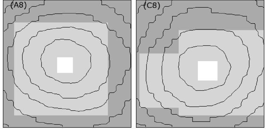
Figure 13: Projections on the $xy$ plane, showing the projected AMR level in a zone with a side of $0.2\ R_{\mathrm{vir}}$, centred at the cluster core, at $z=0$. The colour white corresponds to the AMR level $l=8$, light gray to $l=7$ and dark gray to $l=6$, respectively. Baryon density contours are superimposed. The two panels refer to the runs with maximum AMR level $l_{\mathrm{max}}=8$ and the AMR setup indicated by the letter at the upper left corners.

The rms velocities within the innermost $0.1\ R_{\mathrm{vir}}$ are presented in Fig. 14. For each AMR setup, one can see that $v_{\mathrm{rms}}(l_{\mathrm{max}}=6)<v_{\mathrm{rms}}(l_{\mathrm{max}}=7)$, because the flow structures are less resolved by the coarser grid structure. On the other hand, the runs with $l_{\mathrm{max}}=8$ have a level of rms velocity which is the same as the simulations with $l_{\mathrm{max}}=7$. This is also due to the AMR grid, because the volume coverage of $l=8$ is very limited with the employed refinement criteria (Fig. 13).

Figure 14: Mass-weighted, rms baryon velocity calculated within a sphere with $R=0.1\ R_{\mathrm{vir}}$ centred at the cluster centre at $z=0$, for runs with different AMR maximum levels (indicated on the $y$ axis) and refinement criteria (cf. Table 1). Solid line: AMR criteria as in run $A$. Dotted line: AMR criteria as in run $C$.

It appears therefore that the level of velocity fluctuations in the cluster core, when averaged on a sphere of $R=128\ \mathrm{kpc}\ h^{-1}$, is not affected by setting the effective resolution below $7.8\ \mathrm{kpc}\ h^{-1}$ (AMR level $l=7$). The values of $v_{\mathrm{rms}}$ show a clear convergence for increasing $l_{\mathrm{max}}$. It is interesting to point out that $v_{\mathrm{rms}}(A)<v_{\mathrm{rms}}(C)$ even at $l_{\mathrm{max}}=6$, when the grid coverage of the cluster core is identical for the two AMR setups. From this convergence study we can assert that the effectiveness of the new AMR criteria in resolving turbulent flows does not come trivially from a larger grid coverage, or a larger number of grids, but instead from a more suitable refinement strategy.

Though our simulations show convergence between the AMR levels 7 and 8, one should note that the number of DM particles (and thus the mass of each particle) could affect the results. This issue has not been fully explored in this work, but in a test runs with coarser particle resolution ($64^{3}$ DM particles at $l=0$ and $1$) and AMR setup $A$, we found a velocity dispersion only $5\ \%$ smaller than in run $A$ with $l_{\mathrm{max}}=6$, which formally has the same effective spatial resolution.

5 Summary and conclusions

The study of turbulent flows in the ICM is important for a thorough understanding of galaxy clusters and for the physics of the plasma in these objects. The turbulent state of the ICM is, from an observational point of view, still a debated issue, and the theoretical determination of the kinematic viscosity contains large uncertainties. Besides these open problems, a specific question has been addressed in this work: are the existing numerical techniques of grid-based, AMR cosmological simulations suitable for studying the main properties of turbulence in the ICM? In particular, our attention was focused on the AMR criteria employed in simulations of strongly clumped objects. A galaxy cluster was therefore simulated with a standard, reference setup, and then the simulation was repeated with five different choices of refinement criteria.

The runs were subdivided into two groups, with an underlying difference in the refinement strategy. In the first group, we used AMR criteria based on the regional variability of control variables of the flow, designed for refining the grid at the locations of significant velocity fluctuations. In the second group, a more accurate tracking of the overdense subclumps was enforced.

The distinction between the two groups of runs is important for the interpretation of the results of Sects. 4.2 and 4.3. In the runs $B$, $C$ and $D$, the values of $\max{(|\mn@boldsymbol{\omega}|)}$ (Table 2) and $v_{\mathrm{rms}}$ (Table 3) are larger with respect to run $A$, and to the runs of the second group. The AMR criteria used in these runs are therefore very suitable for refining the grid where the velocity fluctuations are underresolved, and result in an increased magnitude of the turbulence. In the second group of runs, the AMR does not refine explicitly on turbulence, but the lower threshold on overdense region allows a better tracking of subclumps. In other words, the stirring mechanism for turbulence generation in the ICM is better resolved. Therefore comparatively larger $\langle|\mn@boldsymbol{\omega}|\rangle$ and a larger volume-filling factor are obtained.

In both groups of simulations, the results in the innermost $0.1\ R_{\mathrm{vir}}$ are consistent with a better modelling of the turbulent flow. In addition to an increased rms velocity, the change in $P_{\mathrm{turb}}/P_{\mathrm{tot}}$ indicates that the turbulent component plays a non-negligible role in the pressure support. Recently Churazov et al. (2007), based on X-ray and optical observations of M87 and NGC 1399, put a constraint of the order of $10\ \%$ on the non-thermal contribution to the thermal pressure, due to turbulent motions, cosmic rays and magnetic fields. This is not in contradiction to the findings of our work, because we find that the turbulent pressure is only a few percent of the thermal pressure at most.

The presented comparison shows clearly that run $A$ (which implements AMR criteria widely used in grid-based cosmological simulations) fails to reproduce both the magnitude of the rms velocity and the spatial extent of the turbulent flow. This central issue should be carefully taken into account in future investigations of the ICM turbulent features. These results suggest that computationally more demanding simulations will be able to resolve more flow and substructures, which in turn can further contribute to the turbulent properties.

Apparently the presented AMR approach to the modelling of turbulent flows in the ICM has limited utility outside of the cluster core. As discussed in Sec. 4.3, this is partly due to the volume-filling properties of turbulence in clusters, and partly to the constraint on the number of produced AMR grids which, if too many, would make the simulation computationally unaffordable.

The presented results are similar to previous simulations (Norman & Bryan, 1999; Dolag et al., 2005), as far as the magnitude of the turbulent velocity is concerned. Interestingly, Kim (2007) shows that the level of ICM turbulence driven by galaxy motions saturates around 220 km/s, which is not very different from our results. As stated in the Introduction, a detailed comparison of the features of turbulence in SPH and grid-based simulation is out of the scope of this paper, but we observe that the trends that we inferred from Table 3 are also present in Dolag et al. (2005). In that case, when the low-viscosity SPH scheme is used, the variation of some of the variables is more marked that in our study. However it should be stressed that in this work we do not make use of a improved numerical scheme to better resolve turbulence, but only of more suitable choices of AMR criteria.

In many astrophysical problems (including galaxy clusters) the range of length scales needed to follow the turbulent cascade down to the Kolmogorov dissipation scale extends well beyond the grid spatial resolution limit, even using AMR. A strong improvement in the modelling of turbulence would be the application of Large Eddy Simulations, where only the largest scales are resolved and the dynamics at length scales smaller than the spatial resolution is handled by a subgrid scale model (Sagaut, 2001; Schmidt et al., 2006a, b). Such a tool will allow to consistently evaluate the level of subgrid turbulent energy and will make the numerical information about the level of turbulence in the flow more directly available. We expect that the magnitude of the turbulent motions, also outside $0.1\ R_{\mathrm{vir}}$, could be substantially increased. The use of this tool in the framework of cosmological simulations will be explored in future work.

References

- Agertz et al. (2007) Agertz O., Moore B., Stadel J., Potter D., Miniati F., Read J., Mayer L., Gawryszczak A., Kravtsov A., Monaghan J., Nordlund A., Pearce F., et al., 2007, MNRAS, 380, 963
- Braginskii (1965) Braginskii S. I., 1965, Reviews of Plasma Physics, 1, 205
- Bregman & David (1989) Bregman J. N., David L. P., 1989, ApJ, 341, 49
- Brüggen et al. (2005a) Brüggen M., Hoeft M., Ruszkowski M., 2005a, ApJ, 628, 153
- Brüggen et al. (2005b) Brüggen M., Ruszkowski M., Simionescu A., Hoeft M., Dalla Vecchia C., 2005b, ApJ, 631, L21
- Brunetti (2004) Brunetti G., 2004, Journal of Korean Astronomical Society, 37, 493
- Brunetti & Lazarian (2007) Brunetti G., Lazarian A., 2007, MNRAS, 378, 245
- Churazov et al. (2004) Churazov E., Forman W., Jones C., Sunyaev R., Böhringer H., 2004, MNRAS, 347, 29
- Churazov et al. (2007) Churazov E., Forman W., Vikhlinin A., Tremaine S., Gerhard O., Jones C., 2007, ArXiv Astrophysics e-prints (0711.4686)
- Dennis & Chandran (2005) Dennis T. J., Chandran B. D. G., 2005, ApJ, 622, 205
- Dolag et al. (2002) Dolag K., Bartelmann M., Lesch H., 2002, A&A, 387, 383
- Dolag et al. (2005) Dolag K., Vazza F., Brunetti G., Tormen G., 2005, MNRAS, 364, 753
- Eisenstein & Hu (1999) Eisenstein D. J., Hu W., 1999, ApJ, 511, 5
- Eisenstein & Hut (1998) Eisenstein D. J., Hut P., 1998, ApJ, 498, 137
- Enßlin & Vogt (2006) Enßlin T. A., Vogt C., 2006, A&A, 453, 447
- Fabian et al. (2003a) Fabian A. C., Sanders J. S., Allen S. W., Crawford C. S., Iwasawa K., Johnstone R. M., Schmidt R. W., Taylor G. B., 2003a, MNRAS, 344, L43
- Fabian et al. (2003b) Fabian A. C., Sanders J. S., Crawford C. S., Conselice C. J., Gallagher J. S., Wyse R. F. G., 2003b, MNRAS, 344, L48
- Fujita et al. (2004a) Fujita Y., Matsumoto T., Wada K., 2004a, ApJ, 612, L9
- Fujita et al. (2004b) Fujita Y., Suzuki T. K., Wada K., 2004b, ApJ, 600, 650
- Heitmann et al. (2007) Heitmann K., Lukic Z., Fasel P., Habib S., Warren M. S., White M., Ahrens J., Ankeny L., Armstrong R., O’Shea B., Ricker P. . M., Springel V., Stadel J., Trac H., 2007, ArXiv e-prints, 0706.1270
- Iapichino et al. (2008) Iapichino L., Adamek J., Schmidt W., Niemeyer J. C., 2008, MNRAS, accepted (Paper I)
- Jones (2007) Jones T. W., 2007, in ASP Conference Series, Vol. 386, Extragalactic Jets: Theory and Observation from Radio to Gamma Ray, Rector T., De Young D., eds., p. 398, arXiv e-prints: 0708.2284
- Kang et al. (2007) Kang H., Ryu D., Cen R., Ostriker J. P., 2007, ApJ, 669, 729
- Kim (2007) Kim W.-T., 2007, ApJ, 667, L5
- Kim & Narayan (2003) Kim W.-T., Narayan R., 2003, ApJ, 596, L139
- Kritsuk et al. (2006) Kritsuk A. G., Norman M. L., Padoan P., 2006, ApJ, 638, L25
- Kritsuk et al. (2007) Kritsuk A. G., Norman M. L., Padoan P., Wagner R., 2007, ApJ, 665, 416
- Mathis et al. (2005) Mathis H., Lavaux G., Diego J. M., Silk J., 2005, MNRAS, 357, 801
- Miniati et al. (2001a) Miniati F., Jones T. W., Kang H., Ryu D., 2001a, ApJ, 562, 233
- Miniati et al. (2001b) Miniati F., Ryu D., Kang H., Jones T. W., 2001b, ApJ, 559, 59
- Miniati et al. (2000) Miniati F., Ryu D., Kang H., Jones T. W., Cen R., Ostriker J. P., 2000, ApJ, 542, 608
- Narayan & Medvedev (2001) Narayan R., Medvedev M. V., 2001, ApJ, 562, L129
- Norman & Bryan (1999) Norman M. L., Bryan G. L., 1999, in Lecture Notes in Physics, Berlin Springer Verlag, Vol. 530, The Radio Galaxy Messier 87, Röser H.-J., Meisenheimer K., eds., p. 106
- O’Shea et al. (2005a) O’Shea B. W., Bryan G., Bordner J., Norman M. L., Abel T., Harkness R., Kritsuk A., 2005a, in Lecture Notes in Computational Science and Engineering, Vol. 41, Adaptive Mesh Refinement – Theory and Applications, ed. T. Plewa, T. Linde, V.G. Weirs (Berlin; New York: Springer), p. 341
- O’Shea et al. (2005b) O’Shea B. W., Nagamine K., Springel V., Hernquist L., Norman M. L., 2005b, ApJS, 160, 1
- Plewa & Müller (2001) Plewa T., Müller E., 2001, Computer Physics Communications, 138, 101
- Rebusco et al. (2005) Rebusco P., Churazov E., Böhringer H., Forman W., 2005, MNRAS, 359, 1041
- Rebusco et al. (2006) —, 2006, MNRAS, 372, 1840
- Rebusco et al. (2008) Rebusco P., Churazov E., Sunyaev R., Böhringer H., Forman W., 2008, MNRAS, 384, 1511
- Reynolds et al. (2005) Reynolds C. S., McKernan B., Fabian A. C., Stone J. M., Vernaleo J. C., 2005, MNRAS, 357, 242
- Ricker (1998) Ricker P. M., 1998, ApJ, 496, 670
- Ricker & Sarazin (2001) Ricker P. M., Sarazin C. L., 2001, ApJ, 561, 621
- Ryu et al. (2003) Ryu D., Kang H., Hallman E., Jones T. W., 2003, ApJ, 593, 599
- Sagaut (2001) Sagaut P., 2001, Large Eddy Simulation for Incompressible Flows. An Introduction. Springer, Berlin
- Schmidt et al. (2008) Schmidt W., Federrath C., Hupp M., Kern S., Niemeyer J. C., 2008, A&A, submitted
- Schmidt et al. (2006a) Schmidt W., Niemeyer J. C., Hillebrandt W., 2006a, A&A, 450, 265
- Schmidt et al. (2006b) Schmidt W., Niemeyer J. C., Hillebrandt W., Röpke F. K., 2006b, A&A, 450, 283
- Schuecker et al. (2004) Schuecker P., Finoguenov A., Miniati F., Böhringer H., Briel U. G., 2004, A&A, 426, 387
- Sijacki & Springel (2006) Sijacki D., Springel V., 2006, MNRAS, 366, 397
- Spitzer (1962) Spitzer L., 1962, Physics of Fully Ionized Gases. New York: Interscience (2nd edition), 1962
- Springel (2005) Springel V., 2005, MNRAS, 364, 1105
- Subramanian et al. (2006) Subramanian K., Shukurov A., Haugen N. E. L., 2006, MNRAS, 366, 1437
- Sunyaev et al. (2003) Sunyaev R. A., Norman M. L., Bryan G. L., 2003, Astronomy Letters, 29, 783
- Takizawa (2000) Takizawa M., 2000, ApJ, 532, 183
- Vazza et al. (2006) Vazza F., Tormen G., Cassano R., Brunetti G., Dolag K., 2006, MNRAS, 369, L14
- Vogt & Enßlin (2005) Vogt C., Enßlin T. A., 2005, A&A, 434, 67
- Wise & Abel (2007) Wise J. H., Abel T., 2007, ApJ, 665, 899