Links between magnetic fields and plasma flows in a coronal hole

We compare the small-scale features visible in the Ne viii Doppler-shift map of an equatorial coronal hole (CH) as observed by SUMER with the small-scale structures of the magnetic field as constructed from a simultaneous photospheric magnetogram by a potential magnetic-field extrapolation. The combined data set is analysed with respect to the small-scale flows of coronal matter, which means that the Ne viii Doppler-shift used as tracer of the plasma flow is investigated in close connection with the ambient magnetic field. Some small closed-field regions in this largely open CH are also found in the coronal volume considered. The Doppler-shift patterns are found to be clearly linked with the field topology.

1 Introduction

In this study we present observations of an equatorial coronal hole (CH) and investigate the magnetic field structures in the source regions of the fast solar wind. We directly compare the Dopplergrams obtained by the SUMER (Solar Ultraviolet Measurements of Emitted Radiation) instrument, yielding the plasma flow velocity, with the photospheric magnetograms at the bottom of the CH, which via magnetic field extrapolation gives us the coronal magnetic field. In the case studied here we thus combine spectroscopic data with the three dimensional (3-D) magnetic field, an approach providing a clearer physical picture of the plasma conditions and flow pattern prevailing in the corona. This CH was studied before by Xia (2003) and Xia et al. (2003). Therefore we refer the reader to their papers for further details.

The new aspect here is the 3-D magnetic field, which is constructed from magnetograms and extrapolated to all heights above the photosphere. We use the Greens function method to compute the current-free magnetic field from the scalar potential,

$$\Phi({\bf r})=-\frac{1}{2\pi}\int_{\partial\Omega}B_{z}({\bf r^{{}^{\prime}}})\,\frac{d\sigma^{{}^{\prime}}}{|{\bf r}-{\bf r^{{}^{\prime}}}|},\;\;{\bf B}=\nabla\Phi,$$ (1)

where $B_{z}$ is the line-of-sight (LOS) photospheric magnetic field, $\partial\Omega$ denotes the bottom boundary surface (photosphere) of the computational box, $d\sigma=dx\,dy$, ${\bf r}=\sqrt{x^{2}+y^{2}+z^{2}}$, and ${\bf B}({\bf r})$ is the 3-D magnetic field. Details of the extrapolation technique for CHs and the quiet Sun have been described in earlier work by Wiegelmann and Solanki (2004). Potential fields can be reconstructed from the LOS component of the photospheric magnetic field alone. The corresponding measurements are available, e.g., from the MDI (Michelson Doppler Imager) LOS magnetograph data on SOHO.

For the reconstruction of the dynamic coronal magnetic field, such as in twisted loops, it is usually necessary to include the currents, which often are assumed to be parallel to the magnetic field. These force-free magnetic fields are mathematically more difficult to model, and one needs for their reconstruction additional observational input data, such as the photospheric magnetic field vector (Wiegelmann, 2004), or optical images of the coronal plasma structures. This method has been used by Marsch et al. (2004), who carried out a comprehensive study of fields and flows in active regions (ARs) associated with sunspots.

Figure 1: Magnetic structures in a coronal hole. The gray-coding shows the field strength in the photosphere. The black line gives roughly the boundary of the coronal hole. The field of view for SUMER is marked as a red rectangle in both panels. The magnetic field was constructed from a MDI magnetogram. Left figure: mostly closed loops at various scales. Only closed magnetic field lines with $B\geq 30$ G are shown. Right figure: Only open fields with large photospheric values, $B\geq 100$ G. The open flux is bundled in narrow uniform filaments and originates in stronger fields concentrated at small-scale footpoints. The flux tubes expand as they extend into the corona. The average expansion factor (ratio of the maxium to the minimum of the flux tube area) is $28\pm 11$.

2 Data analysis and field extrapolation

During the first week of November in 1999, the SUMER telescope was pointed to a large equatorial coronal hole and traced its darkest parts with raster scans. The selected spectral window was centered around 154 nm, a range which includes the lines of Si ii (153.3 nm), C iv (154.8 nm) and (155 nm), and Ne viii (77 nm) in 2nd order. Their formation temperatures span from about $1.8\times 10^{4}$ K to $6.3\times 10^{5}$ K. The lines are emitted in the upper chromosphere, transition region and lower corona, respectively.

The SUMER data selected for this study were taken on 5 November 1999 and analysed by Xia et al. (2003). The CH discussed here is shown in their Fig.1. The instrument and data analysis techniques are described in detail by Wilhelm et al. (1997). The detector A and slit 2 with a size of 1″$\times$ 300″  were used. SUMER began to raster in the East-West direction at 470″E and ended at 185″E (solar disk coordinates). The corresponding times are 17:07 UT and 21:07 UT, respectively. A 150 s exposure time and 3″  raster step size were selected. The slit’s center was pointed at 100″N during the whole scan. The total data set consists of 96 exposures. Here we use a magnetogram from MDI after Scherrer et al. (1995). The MDI magnetogram, taken at 19:11 UT, has a spatial resolution of 1.98″$\times$1.98″  and was coaligned with the SUMER images. We used the magnetogram with $230\times 254$ pixels and extrapolated the magnetic field into the corona up to a vertical height of $98$″  with the help of the Greens-function method. The magnetic field lines shown in Fig. 1 correspond to a box of $454$″  in $x$, $502$″  in $y$ and $50$″  in $z$, where $z$ is the height above the photosphere. The field lines are stretched in $z$-direction, and we cut off the picture at a height of $50$″  to make the small closed loops visible. The aspect ratio between the vertical and horizontal dimension is 9 to 1.

The results of the extrapolation are illustrated in Fig. 1. Various magnetic field structures in the corona are obvious. The gray-coded bottom plot shows the weak unipolar magnetic field strength in the photosphere, as derived from data of the MDI instrument. The black line delineates the boundary of the coronal hole, as identified in the EUV images obtained by EIT (Extreme Ultraviolet Imaging Telescope) and SUMER on SOHO. Magnetic field lines are treated as open when they reach the upper boundary of our computational box ($98$″). From these extrapolations alone we cannot tell definitely whether the identified open field lines are globally open or close somewhere else on the Sun. Global potential field source surface models have been used to reproduce the location of CHs, but these models do not provide their fine structures and have a source surface (around $2.5R_{\rm S}$) at which the field lines are forced to be open. A comparison of full-Sun EIT-images with global coronal magnetic field in particular for CHs was made by Wiegelmann and Solanki (2004b). This work shows in its Fig. 1 that field lines in spectroscopically identified coronal holes that are open at $100$″  do remain open beyond 2 solar radii to the source surface.

The closed magnetic field lines (yellow) in the left frame of Fig. 1 pertain to photospheric fields with strength $B\geq 30$ G, the open ones (red-brown) in the right frame to stronger fields, with $B\geq 100$ G. Very few field lines are separately shown, to not confuse the picture by intermingling of magnetic field lines, which would produce a diffuse unresolved pattern.

Note that the open magnetic flux (right frame) is concentrated, with linear bundles reaching the top of the simulation box. These bundles are anchored in small (a few seconds of arc in diameter) tubes linked to fine structures with strong unipolar photospheric magnetic flux. Despite their filamentary nature, the flux tubes spread with height, and as coronal funnels fill increasingly larger fractions of the CH at greater altitude.

Not unexpectedly, in the CH there are only low-lying loops. They sparsely populate the hole area, consistent with the statistical results of Wiegelmann and Solanki (2004). Note, in contrast, that the strong loops just outside of the hole reach greater heights. This region also has much brighter ultraviolet emission due to a better plasma confinement and higher plasma density.

The corresponding radiance maps, Ne viii Dopplershifts and magnetograms are shown in Fig. 1 and Fig. 2 of Xia et al. (2003). Here a complementary magnetogram obtained from NSO/Kitt Peak (Jones et al. (1992)), is overlaid with contours of the Doppler shifts in km s^-1 of the Ne viii (77 nm) line.

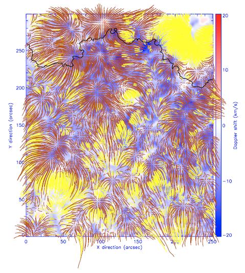
Figure 2: Map of the Doppler shift of the Ne viii (77 nm) emission line, together with the projections of the extrapolated coronal magnetic field lines. Here yellow means closed and red-brown open field lines. An area of 300″$\times$ 250″  on the solar disk is shown, covering a large fraction of the equatorial CH and its boundary regions. Note the uniformly yellow domain in the top right corner, which lies outside the hole and corresponds to closed loops. The cross-shaped spines of open flux in the top left corner coincide with bluish patches and thus indicate sizable coronal plasma outflow in this open field domain, in particular at location (100″,  250″) inside the CH. Outside the CH, e.g. at location (110″,  290″) we find an open field region with hardly any blueshift. Note further that there are many open field lines overarching the yellow patches, corresponding to the closed magnetic carpet with flux confined to near the solar surface.

In Fig. 2 we present the same Dopplermap, with the Doppler shift over the range of $\pm 20$ km s^-1, and the extrapolated magnetic field lines shown in projection for comparison with the Dopplershift pattern. Again the closed field lines are yellow and the open ones red-brown. An area of $250\arcsec\times 300\arcsec$ on the solar disk is shown, covering a large fraction of the equatorial CH and its boundary regions. Note the uniformly yellow domain in the top right corner, which lies outside the hole and corresponds to closed loops shown before in Fig. 1. The cross-shaped spines of open flux, in the top left corner for instance, mostly coincide with bluish patches and thus indicate sizable plasma outflow in this open field domains, in particular at location (100″,  250″). Furthermore, note that there are many open field lines overarching the smaller yellow patches, which correspond to the closed magnetic carpet.

Detailed inspection of Fig. 1, and a comparison with the previously published figures in Xia et al. (2003), indicates that almost everywhere in the present figure do we find Doppler blue shifts, i.e. plasma outflow along the line of sight at speeds of typically up to 10 km s^-1. There are hardly any significant redshifts. In the yellow domain, with closed magnetic flux, the plasma is nearly at rest.

The reader should be aware of alternative explanations of Doppler shifts in terms of wave motion instead of mass flow. For example redshifts in transition region lines were explained as indications of wave motion by Hansteen & Maltby (1994), and blueshifts cannot unequivocally be interpreted as signs of outflow, but may also be related to upward propagating waves.

Figure 3: Magnetic field lines projected on a cut through the extrapolation box in the $y$-$z$-plane for the horizontal coordinate $x=210$″. The small-scale loops at the bottom of the domain tend to push overlaying weaker fields upwards. Note some strongly expanding funnels at $y=40$″  at low heights (below about $10$″). We see that the height of closed loops in the hole (for $x<200$″) is below about $5$″. Outside the hole ($x>200$″) we find closed loops up to a height of about $30$″.

In order to visualize better the fine structures of the magnetic field as a function of height (coordinate $z$) in the corona, we present in Fig. 3 a cut through the box in the $y$-$z$-plane at $x=210$″. This presentation facilitates the clear identification of open and closed (in the simulation box) field lines. The small-scale loops of the magnetic carpet at the bottom of the domain tend to push overarching weaker fields upwards. The overlaid horizontal lines give the level of constant magnetic field pressure (magnetic magnitude squared) to indicate whether the field is uniformly stratified, or if pressure imbalances do exist. However, these spatial variations rapidly decline with height, and above about $20$″  the overall coronal field is more uniform, and horizontally varies merely on larger scales of the size of $100$″.

Close inspection of the previous Fig. 2 shows that the strongest blue shifts are found in the rosette-type rapidly expanding magnetic funnels. These are the sources of coronal plasma outflow and supply of plasma in the CH to the outer corona and solar wind. In regions with closed magnetic loops (both inside and outside the CH) we do not generally observe blueshifts. Several papers (see, e.g., Hassler et al. (1999), Wilhelm et al. (2000), Xia and Marsch (2003)) have addressed the issue of where the solar wind originates, however all previous analyses relied solely on Doppler maps that were grossly correlated with photospheric magnetograms and/or network images obtained in cool chromospheric ultraviolet emission lines. Following the AR study of Marsch et al. (2004), this is a first attempt to correlate in a CH the plasma flow pattern with the 3-D magnetic field structure.

3 Conclusions

The present study has emphasized the need to analyze solar ultraviolet images and spectrogramms or Doppler-shift maps in close connection with the coronal magnetic field, which can routinely be constructed and extrapolated to the outer corona from photospheric magnetograms. The field is the key player in the low-beta corona in constraining plasma flow and guiding the nascent solar wind outflow through open coronal funnels, which according to Fig. 3 have a more complicated geometry at low heights (below about $10$″) than assumed in the models considered by Marsch and Tu (1997) or Hackenberg et al. (2000). The flux tube geometry in the transition region may be of importance to the initial acceleration of the solar wind (see, e.g., Lie-Svendsen et al. 2002).

The results in Fig. 2 are of central importance to appreciate the key role played by the coronal magnetic field. They corroborate previous findings of SUMER, and complement the results published by Xia et al. (2003) and in the thesis of Xia (2003). The Ne viii Doppler-shift maps show a close relationship with the magnetic carpet structure and funnels inside the CH. Largest blue shifts with speeds up to 20 km s^-1 (darkest blue patches) are associated with those regions where intense open magnetic fields of a uniform polarity are concentrated. In contrast, the plasma confined in small loops in the CH does not reveal any significant flow.