Vacancy diffusion in the triangular lattice dimer model

Abstract

We study vacancy diffusion on the classical triangular lattice dimer model, subject to the kinetic constraint that dimers can only translate, but not rotate. A single vacancy, i.e. a monomer, in an otherwise fully packed lattice, is always localized in a tree-like structure. The distribution of tree sizes is asymptotically exponential and has an average of $8.16\pm 0.01$ sites. A connected pair of monomers has a finite probability of being delocalized. When delocalized, the diffusion of monomers is anomalous: $\langle\vec{x}^{2}\rangle\propto t^{\beta}$, with $\beta=0.46\pm 0.06$. We also find that the same exponent $\beta$ governs diffusion of clusters of three or four monomers, as well as the diffusion of dimers at finite but low monomer densities. We argue that coordinated motion of monomer pairs is the basic mechanism allowing large-scale transport at low monomer densities. We further identify a “swap-tunneling” mechanism for diffusion of monomer pairs, where a subtle interplay between swap moves (translations of dimers transverse to their axes) and glide moves (translations of dimers parallel to their axes) plays an essential role.

I Introduction

The statistical mechanics of the lattice dimer model has a long and venerable history Heilmann and Lieb (1972); Kenyon (2002). It is one of the earliest prototypical lattice models where hard constraints play an essential role and that has interesting and deep connections with the Ising model and various kinds of lattice gauge theories Moessner et al. (2001). It has been extensively studied in the setting of random sequential adsorption processes (RSA), both reversible and irreversible Evans (1993). More recently, interests in dimer models have been further boosted by their relevance to the resonance valence bond (RVB) theory of high $T_{c}$ superconductivity Anderson (1987); Rokhsar and Kivelson (1988).

The equilibrium physics of lattice dimer models is already well understood. The partition function of fully packed dimers on any planar lattice can be exactly computed using the Pfaffian method, following a theorem of Kasteleyn Kasteleyn (1961, 1963); Fisher (1961); Temperley and Fisher (1961); Fisher and Stephenson (1963). The case with a nonzero monomer fraction proves to be more difficult and interesting. Both analytic techniques and numerical simulations have been used to attack this problem Fendley et al. (2002); Krauth and Moessner (2003). Previous studies of two-dimensional equilibrium dimer models seem to suggest two universality classes Krauth and Moessner (2003): For bipartite lattices, monomers on different sublattices behave as positive or negative charges, interacting with a logarithmic Coulomb potential of entropic origin. The physics of a finite monomer density system is, therefore, well described by the Debye-Huckle theory of a 2D plasma. For non-bipartite lattices, however, the monomers behave as a weakly interacting gas with extremely short-range correlations. This distinction between bipartite and non-bipartite lattices seems to persist even in three dimensions Huse et al. (2003).

Appropriately defined dynamics of dimers may describe the structural rearrangement in dense anisotropic granular or glassy systems. Furthermore, the fact that the equilibrium physics of the dimer model is well understood makes it particularly convenient for a dynamic study. The similarities between glasses and dense granular systems have long been recognized and explored. Furthermore, recent theoretical studies on the glassy dynamics of lattice models with point-like particles, such as the Kob–Anderson model Kob and Andersen (1993); Toninelli et al. (2004, 2005) and other more exotic models Toninelli et al. (2006); Jeng and Schwarz (2007); Toninelli et al. (2007), have revealed deep connections between kinetic constraints and glassy dynamics, as well as new mechanisms of ergodicity breaking in lattice systems . It is therefore interesting to explore how kinetic constraints affect the diffusion of dimers as well as vacancies in the dimer model. Two studies of single-monomer diffusion in an otherwise fully occupied square lattice have been published recently Bouttier et al. (2007); Poghosyan et al. (2008). Here we focus on the two-dimensional triangular lattice, and study diffusion of both single-monomer and monomer clusters.

I.1 Model and Summary of Results

Our main goal is to characterize, both qualitatively and quantitatively, the diffusion of vacancies, i.e. monomers, in a densely packed lattice dimer model, when the dynamics are subject to hardcore repulsion, as well as to various kinetic constraints. We only allow single dimer moves that do not cause double occupation at any site at any time. This naturally excludes two-dimer dynamics such as those considered in the context of quantum dimer models. Therefore no dimer can move in a fully packed triangular lattice; i.e. the system is completely jammed.

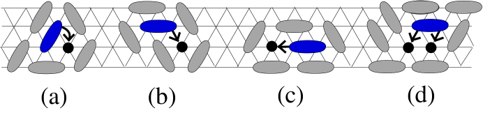
Figure 1: Types of dimer moves. (a) and (b) are rotations, and are not allowed in our model. (c) shows a glide move, and (d) shows a swap move.

A dimer can only move when there are one or more vacancies, i.e. monomers, in its immediate neighborhood. When a dimer has only one nearest monomer, there are two kinds of moves that we could allow: moves in which the dimer changes its orientation as well as its position, which we call a rotation, or moves in which it simply translates along its axis, which we call a glide (see Fig. 1a-c). If both rotations and glides of dimers are allowed, a monomer can always move in any of the six possible directions. Therefore, a single monomer in an otherwise fully occupied triangular lattice simply performs a random walk. At finite monomer density, all monomers simply behave as weakly interacting gas molecules. The dimer diffusion constant scales linearly with the monomer density $\rho_{m}$. Such a scenario is clearly uninteresting.

We shall therefore forbid rotations of dimers from now on . Given an isolated monomer, if there is a nearest dimer with its axis pointing towards the monomer, as shown in Fig. 1c, the dimer can glide into the monomer site. In this case, the monomer moves along one of the three crystal axes by two lattice steps. Therefore, with glide moves a monomer can only move on one of the four sub-lattices of the triangular lattice, shown in Fig. 2. Furthermore, we shall prove in Sec. III that a monomer can never return to its initial lattice site from a different direction than which it left it. Therefore all lattice sites reachable by an isolated monomer form a tree-like structure, which we shall call a monomer tree. Both back-of-the-envelope calculations and numerical simulations indicate that monomer tree sizes are always finite. The distribution of the monomer tree size is asymptotically exponential, as illustrated in Fig. 8, with an average of $8.16\pm 0.01$ sites. We thus expect that single monomer moves do not contribute to the large-scale transport of dimers at high packing density. Consequently, some other collective mechanism is needed for the diffusion of dimers over large length scales.

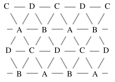
Figure 2: The four sub-lattices in the dimer model.

Now let us consider two monomers which are nearest neighbors to each other . We allow nearby dimers to translate transverse to their axes and occupy the lattice sites of two monomers, as illustrated in Fig. 1d. Such a dimer move shall be called a swap. Swap moves provide a mechanism for changing the monomer tree structures, which is essential for large-scale transport in the triangular lattice dimer model in the high packing density regime. Nevertheless, glide moves separate monomer pairs that are nearest neighbors to each other, and make swap moves unavailable. Once separated, two monomers can form a nearest neighbor pair again only at one or more particular pairs of sites. These reconnection events are clearly suppressed by entropic barriers. We therefore have the following qualitative picture for the diffusion of a two-monomer cluster: each monomer may diffuse on its individual monomer tree, via glide of dimers. This move is entropically preferred, but does not contribute to the large-scale transport of monomers/dimers. Only occasionally, the two monomers meet neighboring sites, whereupon they may be able to travel together by a swap move. Each monomer then discovers a new monomer tree on which it can diffuse.

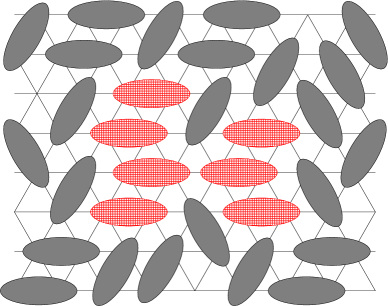
Figure 3: (Color online) A swap cluster. If a two-monomer cluster is created by removing one dimer inside this swap cluster, it can reach all sites in the swap cluster by swap or double-glide moves of dimers.

One might suspect that two-monomer clusters can diffuse faster if we forbid altogether glide moves of dimers. This turns out, however, not to be true. Let us first define a swap cluster in a fully packed lattice as the maximal subset of dimers that have the same orientation, such that if any of these dimers are removed, the resulting connected monomer pair can visit the place of any other dimer in the same cluster by swap moves or double-glide moves, i.e. swap moves or two consecutive glide moves along the same direction. An example of a swap cluster is shown in Fig. 3. We have checked numerically that in the equilibrium ensemble, all swap clusters are finite. As shown in Fig. 4, the distribution of swap cluster sizes is exponential, on average covering $17.89\pm 0.02$ sites. This behavior is of course in qualitative agreement with the extremely short-range correlations exhibited by the equilibrium ensemble of the triangular lattice dimer model.

Now if we create a two-monomer cluster by removing a dimer inside a swap cluster, and only allow swap and double-glide moves, by definition the monomer pair can only visit all the sites of the swap cluster–all sites that are reachable by swap or double-glide move belong to the same swap cluster. That is, the monomer pair is localized if dimer glides are not allowed. Without assistance from other monomers, a monomer pair can escape from a swap cluster only by one mechanism: two monomers may “tunnel” through their individual monomer trees by glide moves and rejoin each other inside some other swap cluster. A configuration in which such tunneling is possible is shown in Fig. 5. Another configuration in which such tunneling is not possible (without first carrying out a swap move) is shown in Fig. 6. We therefore deduce that both glide and swap moves are essential for large-scale diffusion of monomers.

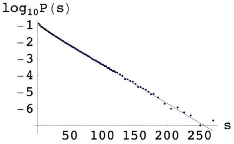
Figure 4: (Color online) Probability distribution of swap cluster sizes. The x-axis measures the number of sites in the swap cluster.

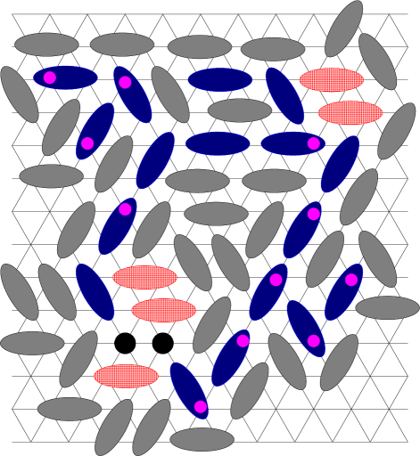
Figure 5: (Color online) A configuration in which two monomer trees touch at a position outside their original swap cluster. The monomer pair starting from the bottom left swap cluster can “tunnel” to the other swap cluster on the top right (to the sites enclosed by the brown circle). The initial and final swap clusters are indicated by the dimers filled with (red) hatched lines. The dark (blue) dimers and the small, light (pink) dots indicate the monomer trees of the individual monomers (see section III).

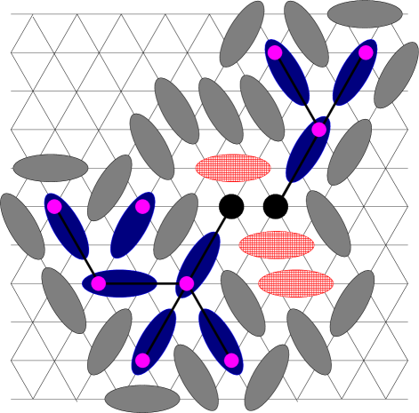
Figure 6: (Color online) A configuration in which two monomer trees touch only at the original positions (two black dots) of the monomers. For this monomer pair to move large distances, the monomers have to meet each other at the two black dots (a reconnection event) and then swap to another location in the swap cluster. The swap cluster is indicated by the dimers filled with (red) hatched lines. The dark (blue) dimers and the small, light (pink) dots indicate the monomer trees of the individual monomers (see section III).

The probability that a monomer pair can escape from a swap cluster depends on the details of dimer packing around the monomer pair. It is not a priori clear whether a monomer pair can diffuse around the whole system by this mechanism. We have run extensive simulations of the diffusion of monomers, and found numerical evidences which show that, when randomly prepared, a finite fraction (about 20%) of monomer pairs are localized, while the remaining fraction can diffuse to infinity. We have also simulated monomer clusters consisting of three or four monomers, and found they are almost always delocalized. Furthermore, we found that in all these cases, the monomer diffusion is anomalous, with an exponent of $0.46\pm 0.05$. We are, however, not able to find a quantitative understanding of this diffusion law. Finally, we have also simulated diffusion of dimers at finite but low monomer densities and discovered also the same anomalous diffusion exponent $\approx 0.47$. This anomalous diffusion of dimers can be understood in terms of diffusion of monomer pairs.

The remainder of this paper is organized as follows. In Sec. II we discuss some details of the model and the numerical method we used in our simulations. In Sec. III we study the diffusion (localization) of a single monomer in an otherwise fully packed lattice. In Sec. IV we present the results on the localization and delocalization of clusters of two, three, or more monomers. In Sec. V we analyze the anomalously slow diffusion of monomers, as well as the statistics of monomer pair reconnection events. In Sec. VI we look at the diffusion of dimers in states with finite monomer density.

II Simulation methods

To prepare the appropriate initial random state of an $L\times L$ triangular lattice packed with dimers, with periodic boundary conditions, we use the pocket algorithm Krauth and Moessner (2003); Krauth (2004, 2006). If we want a configuration with an even number of monomers, we start with a fully packed and fully ordered state (all dimers in the same direction) on an even-by-even lattice; for a configuration with an odd number of monomers, we start with an odd-by-odd lattice that has only one monomer, and that is as nearly fully ordered as possible. We then randomize the state with the pocket algorithm Krauth and Moessner (2003); Krauth (2004, 2006). This algorithm is ergodic, and satisfies detailed balance with respect to the trivially flat measure in configuration space. Each iteration of the algorithm rearranges a large number of dimers, so that the system quickly reaches a random state. A large number of pivots ($5L^{2}$) are carried out to ensure reaching equilibrium. After that, a smaller number of pivots ($10L$) are successively applied to produce other independent random states. It is already known that these random states have only short-range correlations in the dimer orientations Fendley et al. (2002); Krauth and Moessner (2003).

Given a fully packed state (on an even-by-even lattice) or a one-monomer state (on an odd-by-odd lattice), we then generate states with more monomers by removing dimers. When generating states with three or four monomers, we remove dimers adjacent to the already-existing monomers, to create larger monomer clusters.

As stated earlier, in this model dimers can make both glide and swap moves (Fig 1c and d). Once we have an initial state, we carry out these moves. We set the time scale such that, on average, over every unit of time, every dimer attempts one move, choosing at random one of the six possible directions available to it. The attempted move is carried out if and only if it satisfies the hard-core constraint; for an glide move, the site the dimer is moving into needs to be vacant, while for a swap move, both of the sites need to be vacant.

Since we are looking at configurations with low numbers of monomers, generating trial moves by picking among the dimers at random is inefficient. We therefore use the following equivalent, but more efficient algorithm: if we have $N$ monomers, then every step we advance the time by $1/N$, pick a random monomer, and a random site adjacent to that monomer. If the adjacent site is occupied by a dimer that can move into the monomer with an glide move, we do so. If the adjacent site is occupied by a dimer that can move into the monomer with a swap move, we do so with probability 1/2. This generates moves with the same probabilities as if we instead chose random dimers.

III Dynamics of Single Monomer

We first consider configurations with only a single monomer. With only one monomer in the system, swap moves can never occur; only glide moves are allowed. With every glide move, the monomer moves two spaces, so the monomer is confined to one of four sub-lattices—see Fig. 2. This in turn means that a dimer cannot make two glide moves in the same direction—that is, make a glide move in a direction and then, after some moves of other dimers, make a second glide move in the same direction—because it would then be moving into vacancies of different sub-lattices in the two steps, contradicting the result that the monomer remains on the same sub-lattice. This means that with only a single monomer, a dimer is either confined to moving back and forth between two positions, or not moving at all.

This in turn means that for configurations with a single monomer, the latter can never move in a loop (come back to its original lattice site from a different direction than it left that site). Since dimers can only carry out “back and forth” moves, after the monomer leaves its original site by moving a certain dimer, it can only return to its original site from the direction that it left it, by moving the same dimer back to its original position.

This means that for a state with a single monomer, it is easy to quickly figure out which sites the monomer can reach, without explicitly carrying out the dimer moves. We can first see which sites a monomer can reach with a single glide move by inspecting the orientation of dimers on adjacent sites. If a dimer on a neighboring site points towards the monomer, then it can make a glide move into the monomer. Once the monomer makes a single move, it can either move back in the direction that it came from, or make a new move. We can determine what new moves are possible by the same process as before, and thus construct the set of sites that the monomer can reach by repeated glide moves. Since the monomer can never move in a loop, the set of sites that the monomer can reach forms a static tree, such as the one shown in Fig. 7. An isolated monomer thus performs a random walk on its tree.

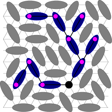
Figure 7: (Color online) A monomer tree. The dark (blue) dimers can eventually move, and the small, light (pink) dots show the sites that the monomer can reach.

Our numerical simulations find that large monomer trees are exponentially suppressed. Fig. 8 shows the distribution of monomer trees sizes for $10^{5}$ configurations on a $101\times 101$ lattice. We stress that for a given configuration, this procedure determines exactly the number of sites that the monomer can visit, so that the distribution in Fig. 8 is exact, up to statistical errors. The average monomer tree size is $8.16\pm 0.01$ sites, and the distribution decays exponentially for large tree sizes, as $\exp(-0.064\,s)$ (where $s$ is the tree size). This implies that in a lattice of infinite size, a single monomer is always localized. At low but finite monomer density, a collective mechanism involving more than one monomers is therefore needed for diffusion of dimers at large length and time scales. This result should be contrasted with a recent similar analysis for the dimer model on the square lattice, which found that single monomers are only weakly localized, having a power law distribution with a diverging expectation value for the number of accessible sites Bouttier et al. (2007).

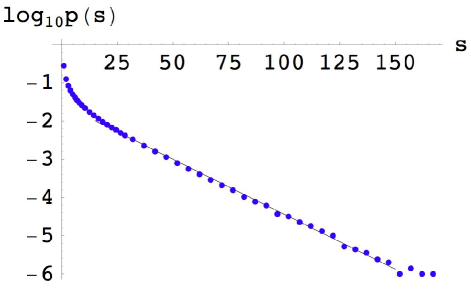
Figure 8: Distribution of monomer tree sizes (the number of sites $s$ a single monomer can reach) in a $101\times 101$ lattice with a single vacancy.

The exponential localization and average monomer tree size on the triangular lattice can be understood by the following heuristic argument. For a configuration with a single monomer, we look at all the sites in the same sub-lattice as the monomer. For the six next-nearest-neighbor sites in the same sub-lattice (sites $A_{1}$ to $A_{6}$ in Fig. 9), we assume that the dimers on those sites each have an independent probability $1/6$ of pointing in any of the six possible directions. This assumption should be fairly good, given the extremely short correlation length of dimer orientations in a fully packed triangular lattice Krauth and Moessner (2003). For each of those sites, if the monomer can reach that site, there are five more sites further out (for example, in Fig. 9, the site $A_{3}$ has neighbors $B_{1}$ through $B_{5}$), each of which we assume has an independent $1/6$ probability of being reachable . Continuing outwards, if we treat the different branches and orientation probabilities as independent, we have site percolation on a Cayley tree, with coordination number $z=6$ and site occupation probability $p=1/6$. In this Cayley tree, the average tree size is $7$, which agrees surprisingly well with our numerical result of $8.16\pm 0.01$. Since cluster sizes for site percolation below the critical point on the Cayley tree are exponentially distributed, our heuristic argument also correctly predicts that large monomer trees are exponentially suppressed.

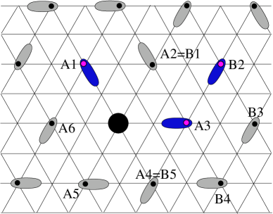
Figure 9: (Color online) Estimate of monomer tree size. We only consider the dimers on sites in the same sub-lattice as the monomer. The dimers drawn are smaller than their actual size in this picture. The blue dimers are movable. The pink dots denote the sites reachable by the monomer (i.e. the monomer tree).

IV Localization of Monomer Clusters

Let us define a monomer cluster to be localized, or confined, if the monomers can only reach a finite number of sites of the system, and delocalized, or deconfined, if some of them can reach an infinite number of sites. Our analysis in the preceding section already shows that single monomers are always localized. In this section, we shall study clusters of monomers.

IV.1 Localization with two monomers

A pair of nearest neighbor monomers can sometimes be localized. For example, in Fig. 10, we show a configuration in which the two monomers can reach only a finite number of sites. It is clear that these two monomers sit on a swap cluster (defined in Sec. I) that contains only two sites. Hence there is no swap move available. Furthermore, it is easy to check that the monomer trees of two monomers touch each other only at the current position of monomers. Each monomer is thus necessarily localized on their individual tree.

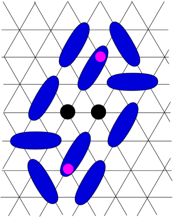
Figure 10: (Color online) A configuration in which two adjacent monomers are confined. The small, light (pink) dots denote sites that can be reached by the monomers.

Our numerical simulations indicate that localization of a monomer pair only happens in roughly one-fourth of the configurations. In contrast to the single-monomer case, however, there is no simple algorithm for determining if a pair of monomers is localized, because the move of one monomer can change the monomer tree of the other, as well as the configuration of swap clusters. Very often, the two monomers appear to be trapped in a region for a long period of time, but after even longer times, the pair finds a way to break out of the region. Additionally, it is also possible that monomer pairs that appear delocalized for a given system size, would in fact be localized, if we considered the system as a subset of an even larger lattice.

We keep track of how many sites have had their occupation changed by a certain time—i.e. the dimer that initially covered the site moved at least once . We say that a configuration of monomers “appears” localized in a region of size $s$ at time $t$ if the number of sites whose occupation has changed is less than or equal to $s$. By creating many random configurations, each with one removed dimer, and running each up to time $t$, we obtain the probability $p_{s}(t)$ that a given configuration with a monomer pair is localized within size $s$ at time $t$, for any $s$. By definition, for a given $t$, $p_{s}(t)$ is a monotonically increasing function of $s$ with $\lim_{s\rightarrow\infty}p_{s}(t)=1$. In the limit $t\to\infty$, $p_{s}(t)$ approaches the probability that a configuration is truly localized within size $s$.

In Fig. 11 we show, for system of size $L=100$ with one monomer pair, $p_{s}(t)$ as a function of $t$, for different values of $s$. It is clear that each curve asymptotes to a nonzero value in the infinite time limit. This indicates that at least a finite fraction of monomer pairs are confined. The asymptotic value $p_{s}(t\rightarrow\infty)$ increases appreciably with $s$, showing that monomer pairs have a broad range of localization sizes.

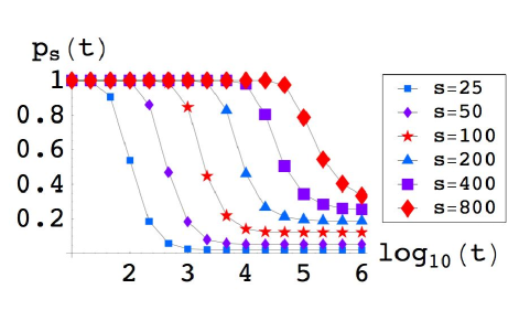
Figure 11: (Color online) Fraction of two-monomer configurations that “appear” to be confined within regions of size $s$ as a function of time. The curves are for increasing $s$ from left to right. The system size is $L=100$.

The derivative of $p_{s}(t)$ with respect to $s$, $\frac{d}{ds}p_{s}(t)$, by definition, is the probability that at time $t$, the number of sites moved is exactly $s$. In Fig. 12 this probability is plotted as a function of $s$, at two different times. The red curve is at $t=10^{5.67}$, and the blue curve is at $t=10^{6}$, again for a system of size $L=100$. It is clear that both curves contain two well separated peaks, a sharp and narrow peak at small $s$, and a secondary, wide peak at a larger value of $s$. The narrow peak at small $s$ does not change with time, implying that the corresponding configurations are indeed localized. By contrast, the wider secondary peak moves outwards with time, suggesting that the corresponding configurations are actually delocalized.

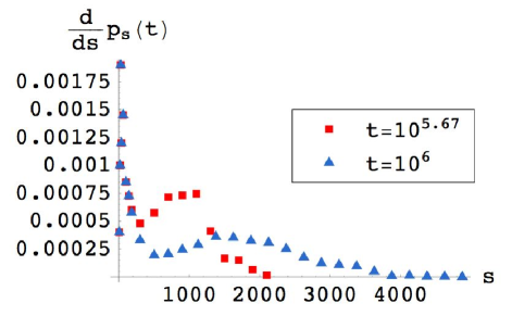
Figure 12: (Color online) The probability that exactly $s$ sites have moved at a given time $t$, for system size $L=100$, and two monomers. This is $\frac{d}{ds}p_{s}(t)$, where $p_{s}(t)$ is shown in Fig. 11. The two curves are for the times $t=10^{5.67}$ and $t=10^{6}$, and lie on top of each other for $s<200$.

While Fig. 12 suggests that there are delocalized states, it is difficult to precisely numerically determine the fraction of configurations that are delocalized. This is because, as already stated, localization is defined in the limit of infinite system sizes and infinite times. Any numerical definition of localization, however, needs to impose arbitrary cutoffs and criteria. For a $240\times 240$ system, we simulated the system for $t=10^{6}$, and numerically defined a state as localized if both the monomers reached no new sites from time $t=10^{5}$ to $t=10^{6}$, and less than half of all sites had their occupation change. With this numerical definition, we found that $21.5\pm 1.3\%$ of the states are localized. This fraction varied as we changed the cutoffs and system size, ranging from 20% to 25%.

Since monomer trees are always of finite size, two monomers in a pair (nearest neighbors in the initial state) cannot be widely separated. In equilibrium, their separation should be proportional to the linear size of monomer trees. In Fig. 13, we see the average monomer-monomer separation as a function of time for a system with two monomers. While the horizontal axis spans six decades of time, the average monomer-monomer separation asymptotes at roughly 6 lattice spacings by $t=10^{4}$. This verifies that monomer pairs are indeed bound. The asymptotic value of 6 lattice spacings is consistent with the average monomer tree size, and does not change as we vary the system size. This result confirms the mechanism presented in Sec. I: A pair of monomers can diffuse only through a two-monomer collective moves, which involves both swap and glide moves.

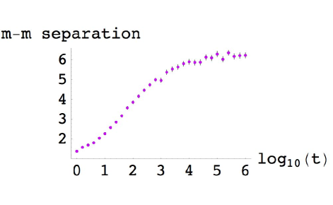
Figure 13: Average separation of a monomer-monomer pair in an otherwise fully packed lattice with $L=240$. This result is insensitive to system size.

While we have not rigorously proven that monomer-pair localization actually happens on infinite lattices with finite probability, our numerical results presented above and in later sections strongly suggest that it is the case. On the other hand, it turns out that the dimer system with only one dimer pair is never ergodic with the constraint of no rotation: There are three orientations of dimers: horizontal, northeastern, and northwestern. The orientation of each dimer is conserved by the dynamics, so the number of dimers with each orientation does not change over time.

Furthermore, it turns out that the system is not even ergodic within a sector with numbers of dimers of each orientation fixed, Recall that the system with $L$ even can be divided into four sub-lattices—see Fig. 2—and that glide moves leave a monomer in the same sub-lattice. Suppose, without loss of generality, that the removed dimer is horizontal, with one monomer in sub-lattice A, and the other in sub-lattice B. Subsequent glide moves will leave the monomers in their sub-lattices. Therefore, wherever the monomers reconnect to one other, they will still form a missing dimer of horizontal orientation. Hence the only possible swap move is to move a horizontal dimer, putting the monomers in sub-lattices C and D respectively (again, see Fig. 2). Likewise, monomers in sub-lattices C and D can also only form missing horizontal dimers. Therefore the dynamics never allow a swap move of a non-horizontal dimer—such dimers can only undergo glide moves. It then follows that along every northeast (northwest) lattice line, the number of northeast-oriented (northwest-oriented) dimers is conserved. For a system with linear size $L$, this means a total of $2L$ conserved quantities.

IV.2 Localization with three or more monomers

The analogues of Figs. 11 and 12 for the three monomer case are shown in Figs. 14 and 15. In Fig. 14, we see that the percentage of states confined in a region of size $s$ appears to go to zero as $t\to\infty$ for any $s$. And in Fig. 15, there is no noticeable localized peak. So the numerical simulations seem to indicate that all states with three connected monomers are delocalized.

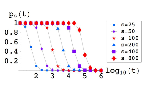
Figure 14: (Color online) Fraction of three-monomer configurations that “appear” to be confined, as a function of time, in regions of size $s$. The curves are for increasing $s$ from left to right. The system size is $L=100$.

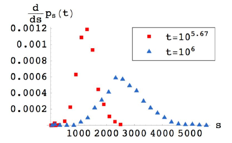
Figure 15: (Color online) The probability that exactly $s$ sites have moved at a given time $t$, for system size $L=100$, and three monomers. This is $\frac{d}{ds}p_{s}(t)$, where $p_{s}(t)$ is shown in Fig. 14. The two curves are for the times $t=10^{5.67}$ and $t=10^{6}$.

It is actually possible, however, for clusters with arbitrary numbers of monomers to be localized. Two such examples for 3-monomer clusters are shown in Figs. 16 and 17. Fig. 18 shows the bottom half of a configuration in which a 4-monomer cluster is confined (the undisplayed top half is identical to the bottom half, up to a rotation of $180^{\circ}$). The latter configuration can be generalized in a straightforward way to arbitrary numbers of monomers in a straight line. In equilibrium, however, localized configurations with three or more connected monomers appear with extremely small (nevertheless remains finite for $L\rightarrow\infty$) probability, and are actually never seen in our simulations. Visual inspection of the dimer dynamics confirms that configurations with a 3-monomer cluster are always delocalized in practice.

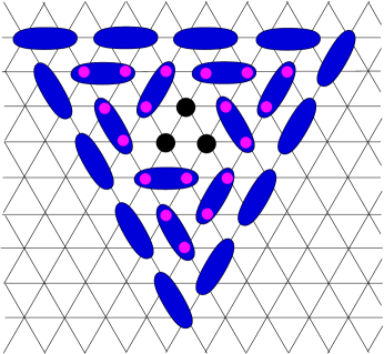
Figure 16: (Color online) A configuration in which three connected monomers are confined. The small, light (pink) dots denote sites that can be reached by the monomers.

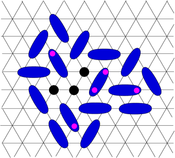
Figure 17: (Color online) A configuration in which three connected monomers are confined. The small, light (pink) dots denote sites that can be reached by the monomers.

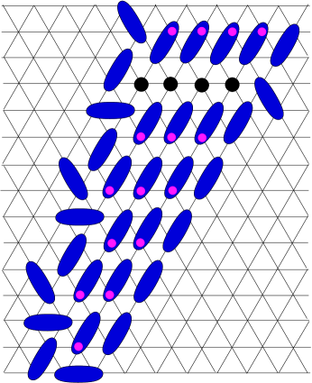
Figure 18: (Color online) Bottom half of a configuration in which four connected monomers in a line are confined. The omitted top half is identical to the bottom half below the four monomers, but rotated $180^{o}$. The small, light (pink) dots denote sites that can be reached by the monomers.

V Anomalous Diffusion of Monomers

Our analysis in the preceding section shows that a single monomer is always localized, while two or three-monomer clusters have finite probability to be delocalized. In this section, we shall characterize the diffusion of these delocalized monomer clusters.

V.1 Diffusion of monomer clusters

Our analysis in the preceding section shows that about 20%-25% of two monomer pairs are localized. We are interested in the diffusion behavior of the delocalized monomer pairs. Unfortunately in numerical simulations, it is difficult to reliably distinguish delocalized cases from localized ones. To avoid this difficulty and obtain better numerical results, we primarily simulated diffusion of three monomer clusters.

We consider the diffusion of monomers with an initial $3$-monomer cluster in a system of size $L=501$. The result is shown in Fig. 19. We averaged over $1500$ independent samples, running each sample for time $t=10^{8.2}$. This simulation took seven days on a computer with a 2.0 GHz processor. We observed anomalously slow diffusion of monomers, with the average displacement square $\langle\vec{x}^{2}\rangle$ scaling as

$$\langle\vec{x}^{2}\rangle\propto t^{\beta}\,,\quad\beta=0.46\pm 0.06.$$ (1)

The data in Fig. 19 shows some deviation from pure power law behavior, but the behavior is clearly subdiffusive over seven decades of time. The error bar in $\beta$ is obtained from the variations in the slope over different time ranges. Simulations with four monomers give a similar curve, with a similar exponent ($\beta=0.44\pm 0.04$), as do shorter simulations with two monomers.

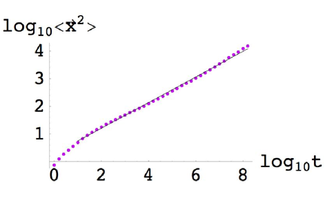
Figure 19: Monomer diffusion at large times. ($L=501$, 3 monomers.)

The initial configurations are prepared by starting with an equilibrium state that is either fully packed, or contains only one vacancy, and then removing random adjacent dimers to form a connected hole. While the fully packed configuration is in equilibrium, however, the configuration generated by the removals is not, as we can see by looking at the average monomer tree size. The monomer tree construction is most useful for a configuration with a single monomer, but we can still define monomer trees for a configuration with multiple monomers, by determining for each monomer the set of sites reachable by glide moves, while holding all other monomers fixed. These trees give a rough characterization of the space available to each monomer, but no longer tell us which sites a monomer can ultimately reach, both because they neglect swap moves, and because each monomer’s moves may change the trees of the other monomers.

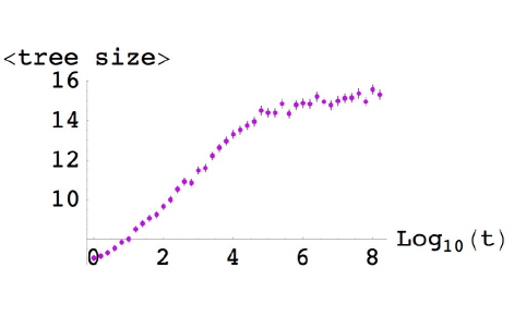
Figure 20: Growth of the average monomer tree size at large times. ($L=501$, 3 monomers.)

In Fig. 20, we see that for a configuration with three monomers, the average tree size grows very slowly (logarithmically) with time, before asymptoting to a roughly constant value. This shows that it takes some time for our initial configuration to reach an equilibrium. The average monomer tree sizes grow in a similar fashion for configurations with 2 or 4 monomers.

To understand how monomer clusters can diffuse at long length scales, let us first consider a configuration with two monomers that are nearest neighbors, such as the configurations shown in Figs. 5 and 6. Numerical simulations show that the individual monomer trees are exponentially distributed, even for configurations with multiple monomers. Hence, glide moves alone are not sufficient to allow a monomer pair to diffuse.

On the other hand, if we prohibit single glide moves and only allow swap moves and double-glide moves (including the latter since they leave the monomers connected), then monomer pairs are always confined to their swap cluster (defined in Sec. I). Numerical simulations show that the swap cluster is also exponentially distributed, with an average of $17.89\pm 0.02$ sites—the distribution is shown in Fig. 4. Therefore, swap moves alone are also not sufficient to allow a monomer pair to diffuse. Hence both glide and swap moves are essential to large-scale diffusion of monomer clusters.

For a two-monomer configuration, such as shown in Figs. 5 and 6, the two monomers can either glide separately along their individual monomer trees, or move together by swap moves. It is clear, however, that immediately after a glide move takes place, the two monomers stop neighboring each other and swap moves are no longer possible. Subsequently, the two monomers perform separate random walks on their own monomer trees, much like isolated monomers in an otherwise fully packed lattice. This situation remains true so long as two monomers do not become nearest neighbors, an event which we shall call “reconnection of a monomer pair”. For large monomer trees, the probability of a reconnection at any given time is small. After reconnecting, a swap move necessarily changes the structure of the monomer trees. The monomer can then perform random walks in their new monomer trees, until they eventually reconnect again. It is clear from this picture that for most of the time steps, the two monomers remain separated, performing random walks on their individual trees. A monomer pair has to overcome entropic barriers (log of monomer tree sizes) in order to reconnect and perform swap moves. This entropic barrier partially explains the slow diffusion seen in the simulations.

There are two possible ways that two monomers can reconnect: a) If the two monomer trees touch each other only in one place, as in Fig. 6 then the only way for two monomers to reconnect is for each of them to, at exactly the same time, go back to the original sites where they separated. After reconnecting, they then with finite probability perform swap moves, changing the monomer trees. The two monomers then may separate again and perform random walks in their new trees. b) If two monomer trees touch at more than one place (multiple junctions), as shown in Fig. 5, then the two monomers may reconnect if they arrive at any of these places simultaneously. Here the most interesting possibility is that two monomers may reconnect inside a swap cluster different from the one they started with. This possibility provides a mechanism for a monomer pair to “tunnel” between different swap clusters, not unlike a Cooper pair tunneling between neighboring superconducting grains.

A monomer pair would be able to diffuse at large length and time scales only if these tunneling events happen with sufficiently high probability. To characterize this probability, we start from a random fully packed configuration, remove a single dimer randomly, and numerically check the number of reconnection sites, i.e. number of contacts between two monomer trees. We find that $38.7\pm 0.1\%$ of the time, the two monomer trees touch only at the original locations of the monomers (as in Fig. 6), while $36.0\pm 0.1\%$ of the time, there is another location where the monomers can meet. However, the quantitative relation between these probabilities and the diffusion behavior of monomers is not easy to obtain.

This “swap-tunneling” mechanism is responsible for $2$-monomer diffusion, but it is unclear whether this mechanism is also responsible for monomer diffusion in a system at low monomer density. To explore this issue, we have also simulated the diffusion of larger monomer clusters. Visual inspection of the diffusion dynamics shows that 1) For a three-monomer cluster, most of the time two monomers remain relatively close to each other and are mutually connected by glide moves, while the third one is very often far away. Furthermore, a three-monomer cluster is always localized if no swap moves are allowed, or if glide moves are not allowed. Therefore it appears that the two monomer “swap-tunneling” dynamics dominates the diffusion of a three-monomer cluster. 2) Our numerical simulations clearly show that monomer clusters of six or fewer connected monomers are localized if swap moves are prohibited. This strongly suggest the importance of swap move in large-scale diffusion of monomer clusters. 3) Four-monomer clusters can be delocalized even if glide moves are disallowed, showing that swap moves alone provide a mechanism for monomer diffusion at low monomer density. However, visual inspection of the simulations shows that when both swap and glide moves are allowed, larger clusters of (four or more) monomers tend to separate into smaller clusters containing one or two monomers. This separation is entropically favorable: there are many more possible glide moves than possible swap moves. More importantly, it shows that the “swap-tunneling” mechanism of two-monomer clusters is indeed the most important mechanism for the large-scale transport of monomers at high packing densities. This conclusion is also supported by our study of dimer diffusion at low by finite monomer density, discussed in Sec. VI.

V.2 Reconnection times

The argument of the preceding subsection indicates that in order for a monomer pair to diffuse, it is essential for the two monomers to reconnect in a different swap cluster. We now study the distribution of time separations between successive reconnection events for pairs of monomers in more detail. Let us first define precisely reconnection events for configurations with only two monomers. Suppose that at time $t_{i}$, the two monomers are on neighboring sites. We identify their swap cluster, and then allow the system to evolve. We say that a reconnection event happens at time $t_{i+1}$ if at this time step the two monomers lie on neighboring sites in a different swap cluster than at time $t_{i}$. We define the time difference $\tau_{i}\equiv t_{i+1}-t_{i}$ as the reconnection time. We then recalculate the new swap cluster of the monomer pair, and repeat the process. To make sure that we study the equilibrium properties of the system with a monomer pair, we simulate the system for a long amount of time ($t_{\rm init}$), before collecting a sequence of reconnection times for a smaller time window ($t_{\rm coll}$). The distribution of reconnection times thus obtained is shown in Fig. 21.

There is a simple way to understand this reconnection time distribution: When we have two connected monomers, each will have its own monomer tree, with sizes $\ell_{1}$ and $\ell_{2}$ respectively. Let us assume that these two trees are identically and independently distributed, each with the probability distribution

$$p(\ell)=\ell^{-a}e^{-\ell/b}.$$ (2)

The above parameters $a$ and $b$ shall be determined by fitting the curve and may be slightly different than those for the isolated monomer case. We further assume that after two monomers separate, each of them quickly independently equilibrates in its own tree, and that the two trees touch at $m$ points in other swap clusters, where $m$ is some fixed number (i.e. does not scale with $\ell_{1}$ and $\ell_{2}$).

Under these assumptions, at any given time, the probability that the two monomers are adjacent is $m/(\ell_{1}\ell_{2})$. The probability that they reconnect for the first time at time $\tau$ (an integer) is thus

$$\left(1-\frac{m}{\ell_{1}\ell_{2}}\right)^{\tau-1}\frac{m}{\ell_{1}\ell_{2}}\approx\frac{m}{\ell_{1}\ell_{2}}e^{-\frac{m\tau}{\ell_{1}\ell_{2}}}.$$ (3)

Averaging over the distributions of $\ell_{1}$ and $\ell_{2}$, we get the probability of first reconnecting at time $\tau$ to be

$$\int d\ell_{1}\int d\ell_{2}\ p(\ell_{1})p(\ell_{2})\frac{m}{\ell_{1}\ell_{2}}e^{-\frac{m\tau}{\ell_{1}\ell_{2}}}.$$ (4)

Note that this is, by definition, the distribution of reconnection times for a monomer pair.

Performing saddle point approximations for both the $\ell_{1}$ and $\ell_{2}$ integrals in Eq. (4), we find that the distribution of reconnection times is proportional to

$$\tau^{-(2a+1)/3}\exp\left(-\frac{3(m\tau)^{1/3}}{b^{2/3}}\right).$$ (5)

In Fig. 21, we see that the distribution is indeed fit well with such a stretched exponential, $\tau^{-\alpha}\exp(-\beta\tau^{1/3})$, with $\alpha=1.13\pm 0.04$, and $\beta=0.30\pm 0.02$. If we fit the single-monomer distribution in Fig. 8 with Eq. 2, we get $a=1.4$ and $b=13$; if we then assume $m=1$, we get $\alpha=1.27$, and $\beta=0.54$, which matches the fitted values reasonably well, given the approximations made.

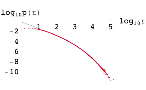
Figure 21: The distribution of reconnection times, fitted to a stretched exponential, $\tau^{-\alpha}\exp(-\beta\tau^{1/3})$, with $\alpha=1.13\pm 0.04$, and $\beta=0.30\pm 0.02$.

We may try to understand the anomalous diffusion of monomer pairs in terms of sporadic swap moves and tunneling, separated by glide moves that do not contribute to large-scale diffusion (separating out the glide moves that make up the tunneling events from those that do not). The reconnection time therefore behaves much like the waiting time for a particle diffusing in a random potential landscape with traps at each site, which separate succeeding hops. It is well known that a waiting time distribution with a diverging average naturally leads to anomalous diffusion Bouchaud and Georges (1990). In our case, however, the average of the reconnection-time distribution (a stretched exponential) is clearly finite. We therefore conclude that the distribution of reconnection times that we see in our simulations does not qualitatively explain the anomalous diffusion of monomers.

We have also analyzed the correlation function of the reconnection time sequences. For a given sequence $\{\tau_{1},\tau_{2},\tau_{3},\ldots\}$ of reconnection times, the correlation function is defined to be

$$C(j) \equiv \langle\tau_{i+j}\tau_{i}\rangle-\langle\tau\rangle^{2},$$ (6)

$$C(\omega) = {\frac{1}{\sqrt{M}}}\sum_{j=1}^{M}e^{i\omega(j-1)}C(j)\quad,$$ (7)

where $M$ is the maximum value of $j$, the correlation distance. The correlation function in frequency space, as shown in Fig. 22 for two different collection time windows (values of $\{t_{\rm init},t_{\rm coll}\}$), depends on the frequency as a power law. While the prefactor of the correlation function depends on the time window, the slope does not. In the frequency space, the correlation function scales as

$$C(\omega)\propto\omega^{-(1-\gamma)},\quad\gamma=0.14\pm 0.01.$$ (8)

This long-range correlation in reconnection times should be related to the anomalous diffusion behavior of monomers. In particular, it may be related to the probability of a monomer pair revisiting its initial swap cluster. A quantitative understanding of this correlation, however, is still lacking.

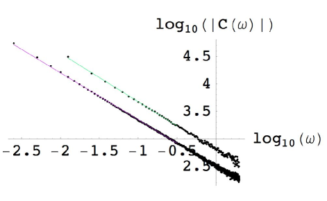
Figure 22: Correlations between reconnection times, in frequency space. The upper (green) curve is for $\{t_{\rm init},t_{\rm coll}\}=\{7.5\times 10^{4},2.5\times 10^{4}\}$, while the lower (purple) curve is for $\{t_{\rm init},t_{\rm coll}\}=\{7.5\times 10^{5},2.5\times 10^{5}\}$. $t_{\rm init}$ is the time used to equilibrate, and $t_{\rm coll}$ is the time window for measurement. Both curves are for $L=250$.

VI Dimer diffusion at finite monomer densities

Our study of monomer diffusion suggests that coordinated “swap-tunneling” motion of monomer pairs constitutes the basic mechanism for diffusion of monomer clusters. In this section, we study diffusion of dimers at finite but low monomer density and show that it can also be understood in terms of monomer pairs.

The first question we need to address is, for a given monomer density, what is the density of monomer pairs? Let us define that two monomers form a pair if they, with all other monomers fixed, can be made nearest neighbors by glide move of dimers. Clearly this is possible if and only if two monomer trees touch each other at one or more sites, as illustrated in Figs. 5 and 6.

A rough estimate of the probability that a second monomer touches a given monomer tree can be obtained as follows. We first want to count the number of distinct neighbors of the sites in the monomer tree. The site that the monomer begins at has $6$ neighbors. Each new site in the tree adds $5$ new neighbors (as one neighbor along the edge of the tree has already been counted). The new neighbors may not all be distinct, since sites of the tree may have overlapping neighbors not on the edges of the tree. Ignoring such overlapping cases, and using the fact that the average size of monomer trees is $8.16$, we get we have $6+5(7.16)\approx 42$ neighbors. If we further assume that monomer positions are independent and uncorrelated , then the probability that the given monomer forms a pair with some other monomer is $1-(1-\rho_{m})^{42}$.

To test this simple estimate, we generate random configurations at finite monomer densities using the pivot algorithm, and count the total number of monomer pairs. As shown in Fig. 23, the numerical results for the probability that a monomer is in a pair agree well with this formula (never differing by more than a factor of $2$, even at the lowest density tested, $\rho_{m}=0.0005$). A better fit, $1-(1-\rho_{m})^{60}$, also shown in Fig. 23, can be obtained by varying the effective number of tree neighbors.

We find that at a monomer density of around $2\%$, the majority (about $70\%$) of monomers already form pairs. On the other hand, at much lower monomer densities, the probability that a given monomer forms a pair with some other monomer is linear in $\rho_{m}$. Therefore for $\rho_{m}\ll 0.02$, the monomer pair density scales as $\rho_{m}^{2}$, while for $\rho_{m}\gg 0.02$, the monomer pair density scales as $\rho_{m}$.

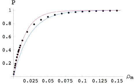
Figure 23: The probability that a given monomer is in a pair with some other monomer, as a function of the monomer density. The lower curve is $1-(1-\rho_{m})^{42}$, and the upper curve is $1-(1-\rho_{m})^{60}$.

To study dimer diffusion, we generate equilibrium configurations at a finite monomer density using the pivot algorithm. We then evolve the system, keeping track of the value of $\langle\vec{x}_{i}^{2}\rangle$ for each dimer, summing over all dimers (including those never moved) in the configuration, and averaging over different configurations. A representative plot of results for $\rho_{m}=0.004$ is shown in Fig. 24. The short time behavior (for $t\leq 10^{2}$) is dominated by glide moves of monomers on their individual trees. At longer time scales (for $10^{3}\leq t\leq 10^{6}$), we find the scaling

$$\langle\vec{x}^{2}\rangle=k\,t^{\tilde{\beta}},\hskip 8.53581pt\tilde{\beta}=0.47\pm 0.02.$$ (9)

We have also simulated monomer densities between $0.0005$ and $0.015$, and found that $\tilde{\beta}$ is roughly constant. For larger $\rho_{m}$, $\tilde{\beta}$ increases with $\rho_{m}$, reaching $0.9$ for $\rho_{m}=0.4$.

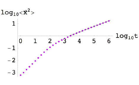
Figure 24: The average dimer displacement squared scales as $\langle\vec{x}^{2}\rangle=k\,t^{0.47}$, averaging over both configurations and dimers, for a $241\times 241$ system with $\rho_{m}=0.004$.

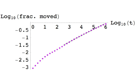
Figure 25: The fraction of dimers that have moved at least once, as a function of time, for a $241\times 241$ system with $\rho_{m}=0.004$.

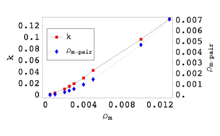
Figure 26: The coefficient $k$ in $\langle\vec{x}^{2}\rangle=k\,t^{\tilde{\beta}}$ for diffusion of dimers (squares, left axis), and the density of monomer pairs, $\rho_{m-pair}$ (diamonds, right axis), each as a function of monomer density $\rho_{m}$. The ratio between these two quantities is roughly constant, varying by a factor less than $3$, while $\rho_{m}$ changes by two orders of magnitude.

We note that this dimer diffusion exponent $\tilde{\beta}\approx 0.47$ measured at low $\rho_{m}$ equals the monomer diffusion exponent $\beta=0.46\pm 0.06$ found in Eq. 1 within numerical precision. This supports our physical picture that diffusion of monomer pairs is the dominating mechanism of large scale transport. At sufficiently low monomer densities ($\rho_{m}\leq 0.02$, for example), the monomer pair density is extremely low. Within reasonable time scales, then, dimer pairs remain well separated and do not touch each other. Hence we can treat the diffusion of each monomer pair separately. As time evolves, monomer pairs diffuse around their original positions. The radius squared of the region that the monomer pair visits scale as $t^{\beta}$, according to our simulation of monomer diffusion (Eq. 1). If this region is compact (correct for 2d diffusion problems), the area of the region visited by a monomer pair should scale with the same exponent. Note that only dimers inside this region have moved. By contrast, dimers outside these regions are frozen at this particular time scale. Hence the system consists of growing “active” regions that have been visited by the monomer pairs, surrounded by “inactive” background. Hence the number of dimers that have moved is the same as the total area of these active regions, which scales as the total number of active regions multiplied by $t^{\beta}$. Consistent with this, we have verified that the number of dimers moved scales as $t^{\beta}$, for all monomer densities—a representative plot is shown in Fig. 25. If we further assume that dimers within each active region on average diffuse up to distances of order of one, then this is also the scaling behavior of dimer diffusion $\langle\vec{x}^{2}\rangle$, given by Eq. (9), hence $\tilde{\beta}=\beta$.

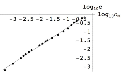
Figure 27: The coefficient $c$ in $\langle r\rangle=c\,t^{\delta}$ for dimer diffusion, averaging over dimers and over configurations, at long times, as a function of monomer density. The straight line fit has a slope of $0.992\pm 0.013$.

As a byproduct, this argument also predicts that the coefficient $k$ in Eq. (9) should be linear in monomer pair density. In Fig. 26 we plot both $k$, and the density of monomer pairs, $\rho_{m-pair}$, as functions of $\rho_{m}$, for low $\rho_{m}$. We see that both graphs are qualitatively similar. While both $k$ and $\rho_{m-pair}$ vary by a factor of $100$ as we vary $\rho_{m}$ from $0.0005$ to $0.013$, the ratio between the two varies by less than a factor of $3$. We thus conclude that the variation of the monomer pair density is primarily responsible for the variation of $k$, and that monomer pairs are indeed responsible for large-scale transport of dimers.

We have also looked at the averaged dimer displacement $\langle r\rangle=\langle|\vec{x}|\rangle$ (rather than the average of displacement squared) at finite monomer densities. We again focus on the behavior at larger times, and fit the results to

$$\langle r\rangle=c\,t^{\delta}.$$ (10)

Surprisingly, we find that $\delta$ is very close to the monomer diffusion exponent $\beta$, varying in the range $0.450\pm 0.025$, for all monomer densities studied in the range of $0.0005<\rho_{m}<0.40$. The equality of the exponent $\delta$ with the exponent $\beta$ of Eq. 1 is expected for low $\rho_{m}$, by the same arguments we presented earlier. However, at higher monomer densities, we find no reason why the exponent $\delta$ in Eq. (10) should remain unchanged—at these densities, most monomers form pairs and the physical picture where the space consists of isolated active regions embedded in an inactive background, is no longer valid. Most dimers end up moving by the onset of anomalous diffusion of dimers. Probably even more puzzling is that the coefficient $c$ in Eq.(10) is linear in $\rho_{m}$ over three decades in $\rho_{m}$, as shown in Fig. 27. The best fit line on a log–log scale has a slope of $0.992\pm 0.013$, indicating a linear dependence of $c$ on $\rho_{m}$. An understanding of this scaling behavior is lacking.

VII Conclusion

In this work we have studied anomalous diffusion of monomers and dimers in the triangular lattice dimer model, subject to the constraints that dimers cannot rotate and that each site can only be occupied by one dimer. We have identified monomer pairs as the basic degree of freedom for large-scale transport of monomers and dimers, and have proposed a “swap-tunneling” mechanism that involves a subtle interplay between swap moves and glide moves. A quantitative understanding of the anomalous exponent for monomer diffusion, however, remains elusive. It will be interesting to further explore whether this intricate vacancy dynamics is relevant to vacancy diffusion in glassy systems as well as in densely packed granular aggregates. Finally we note that our model exhibits no equilibrium jamming transition at finite monomer density: As long as monomer density is finite, there is always probability one to find two-monomer clusters (as well as larger clusters) in an infinite system. According to the results of our work, then, dimers always diffuse anomalously as Eq. (9), at time scales longer than $10^{3}$. At even longer time scales, monomer clusters with large sizes come into effects and dimers may eventually diffuse normally.