Polarized Structure Function $\sigma_{LT^{\prime}}$ for $p({\vec{e}},e^{\prime}K^{+})\Lambda$ in the Nucleon Resonance Region

Abstract

The first measurements of the polarized structure function $\sigma_{LT^{\prime}}$ for the reaction $p(\vec{e},e^{\prime}K^{+})\Lambda$ in the nucleon resonance region are reported. Measurements are included from threshold up to $W$=2.05 GeV for central values of $Q^{2}$ of 0.65 and 1.00 GeV², and nearly the entire kaon center-of-mass angular range. $\sigma_{LT^{\prime}}$ is the imaginary part of the longitudinal-transverse response and is expected to be sensitive to interferences between competing intermediate $s$-channel resonances, as well as resonant and non-resonant processes. The results for $\sigma_{LT^{\prime}}$ are comparable in magnitude to previously reported results from CLAS for $\sigma_{LT}$, the real part of the same response. An intriguing sign change in $\sigma_{LT^{\prime}}$ is observed in the high $Q^{2}$ data at $W\approx 1.9$ GeV. Comparisons to several existing model predictions are shown.

I Introduction

The study of the electromagnetic production of strange quarks in the resonance region plays an important role in understanding the strong interaction. The $p(e,e^{\prime}K^{+})\Lambda$ reaction involves the production of the strange particles $\Lambda$($uds$) and $K^{+}$($u\bar{s}$) in the final state via strange quark-pair ($s\bar{s}$) creation. The fundamental theory for the description of the dynamics of quarks and gluons is known as quantum chromodynamics (QCD). However, while numerical approaches to QCD in the medium-energy regime do exist, neither perturbative QCD nor lattice QCD can presently predict hadron properties seen in this type of reaction. In the non-perturbative regime of nucleon resonance physics, the consequence is that the interpretation of dynamical hadronic processes still hinges to a significant degree on models containing some phenomenological ingredients. Various quark models (see for example Refs. isgur ; capstick1 ; capstick2 ; capstick3 ) predict a large number of non-strange baryons that can decay into a strange baryon and a strange meson, as well as N$\pi$/N$\pi\pi$ final states. While many of these excited states have been observed in pion production data, a large number are “missing”. The higher threshold for $K^{+}\Lambda$ final states kinematically favors production of the missing resonances with masses near 2 GeV. Studies of different final states, such as the associated production of strangeness, can provide complementary information on the contributing amplitudes.

In the absence of direct QCD predictions, effective models must be employed. Utilizing these models by means of fitting them to the available experimental data – cross sections and polarization observables – or comparing the data to the model predictions, can provide information on the reaction dynamics. In addition, these comparisons can provide important qualitative and quantitative information on the contributing resonant and non-resonant terms in the $s$, $t$, and $u$ reaction channels (see Fig. 1). The development of these theoretical models has been highly based on the availability of the experimental data. Precise measurements of cross sections and polarization observables are crucial for the refinement of these models and for the search for missing resonances.

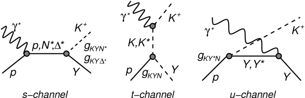
Figure 1: Feynman diagrams representing $s$-channel nucleon ($p,N^{*},\Delta^{*}$) exchange (left), $t$-channel kaon ($K,K^{*}$) exchange (middle), and $u$-channel hyperon ($Y,Y^{*}$) exchange (right) that contribute to the reaction models. The vertex labels $g_{MBB}$ represent the strong coupling constants.

In this paper, we report the first-ever measurements of the longitudinal-transverse polarized structure function, $\sigma_{LT^{\prime}}$, for the $p(\vec{e},e^{\prime}K^{+})\Lambda$ reaction in the resonance region, using the CEBAF Large Acceptance Spectrometer (CLAS) in Hall B of Jefferson Lab. This observable provides complementary information to the $\sigma_{LT}$ structure function reported in Ref. 5st , as will be discussed. Thus, these new data provide another constraint on model parameters, and therefore, provide additional important information in understanding the process of electromagnetic production of strangeness.

There is a growing body of high-quality data on the electromagnetic production of strange hadrons. Recently published data using electron beams exist on the separation of the longitudinal and transverse structure functions, $\sigma_{L}$ and $\sigma_{T}$, from Hall C of Jefferson Lab for both $K^{+}\Lambda$ and $K^{+}\Sigma^{0}$ final states at $W$=1.84 GeV, for $Q^{2}$ up to 2.0 GeV², at a kaon center-of-mass scattering angle of $\theta_{K}^{*}=0^{\circ}$ gabriel ; mohring . The CLAS Collaboration has recently produced results in which unpolarized cross sections and interference structure functions ($\sigma_{TT}$ and $\sigma_{LT}$) have been measured for $K^{+}\Lambda$ and $K^{+}\Sigma^{0}$ final states over a wide kinematic range with $Q^{2}$ up to 2.6 GeV², $W$ up to 2.4 GeV, and nearly complete angular coverage in the center-of-mass frame 5st . These results include the first-ever separation of $\sigma_{L}$ and $\sigma_{T}$ at angles other than $\theta_{K}^{*}=0^{\circ}$. The same set of data has been analyzed to extract the polarization transfer from the virtual photon to the produced $\Lambda$ hyperon carman and to extract the ratio of $\sigma_{L}/\sigma_{T}$ at $\theta_{K}^{*}=0^{\circ}$ for the $K^{+}\Lambda$ final state raue05 . Older electroproduction data from various labs also exist brown ; bebek1 ; azemoon ; bebek2 ; brauel , but with much larger uncertainties and much smaller kinematic coverage.

Complementary data from photoproduction are also available. The SAPHIR collaboration has published total and differential cross section data for photoproduction of $K^{+}\Lambda$ and $K^{+}\Sigma^{0}$ final states with photon energies up to 2 GeV saphir1 ; saphir2 . CLAS has provided extensive differential cross sections mcnabb ; bradford1 , along with recoil mcnabb and transferred polarization bradford2 data for the same final states in similar kinematics. Finally, the LEPS collaboration has measured differential cross sections and polarized beam asymmetries with a linearly polarized photon beam for energies up to 2.4 GeV at forward angles zegers ; sumihama .

The SAPHIR cross section data show an interesting resonance-like structure in the $K^{+}\Lambda$ final state around $W$=1.9 GeV. A similar structure has been seen in the unpolarized electroproduction cross section data 5st , as well as in the photoproduction measurements of CLAS mcnabb ; bradford1 . Within the isobar model of Mart and Bennhold d13mart ; mart , that structure was interpreted as a $D_{13}(1895)$ resonance, which had been predicted by several quark models (e.g. Ref. capstick3 ), but not well established. However, the isobar model of Saghai saghai found that the cross section data could be satisfactorily described without the need for including any new $s$-channel resonances by including higher-spin $u$-channel exchange terms. The need to include the missing $D_{13}(1895)$ state, however, was supported by the new Regge plus resonance model from Ghent ghent that compared their model to a broad set of cross section and polarization observables from the available photo- and electroproduction data.

The organization of this paper includes an overview of the relevant formalism in Section II, a description of the theoretical models used to compare against the data in Section III, details on the experiment and data analysis in Section IV, and a presentation and discussion of the results in Section V. The conclusions are given in Section VI.

II Formalism

A schematic diagram of $K^{+}\Lambda$ electroproduction off a fixed hydrogen target is shown in Fig. 2. The angle between the incident and scattered electron is $\theta_{e}$, while the angle between the electron scattering plane and hadron production plane is defined as $\phi$. In the one-photon exchange approximation, the interaction between the incident electron beam and the target proton is mediated by a virtual photon, $\gamma^{*}$. The virtual photon four momentum is obtained from the difference between the four momenta of the incident, $e=(E,\mathbf{p}_{e}\rm)$, and scattered electrons, $e^{\prime}=(E^{\prime},\mathbf{p}^{\prime}_{e}\rm)$, as:

$$q=e-e^{\prime}=(\nu,\mathbf{q}).$$ (1)

The four momentum transfer squared, $Q^{2}$, is an invariant quantity defined as:

$$Q^{2}=-q^{2}=-(\nu^{2}-\mathbf{q}^{2})=4EE^{\prime}\sin^{2}(\theta_{e^{\prime}}/2),$$ (2)

where $\nu=E-E^{\prime}$ is the energy transfer and $\theta_{e^{\prime}}$ is the electron scattering angle in the lab frame. The invariant mass $W$ of the intermediate hadronic state is defined as:

$$W^{2}=s=M^{2}+2M\nu-Q^{2},$$ (3)

where $M$ is the mass of the proton target.

Figure 2: (Color online) Kinematic diagram for kaon-hyperon ($KY$) electroproduction.

Following the notation of Refs. akerlof ; zeit , the differential cross section for $KY$ electroproduction in the center-of-mass frame is given by:

$$\frac{d\sigma}{dE^{\prime}d\Omega_{e}^{\prime}d\Omega_{K}^{*}}=\Gamma\frac{d\sigma}{d\Omega_{K}^{*}},$$ (4)

where $\Gamma$ is the virtual photon flux given by:

$$\Gamma=\frac{\alpha}{4\pi^{2}}\frac{E^{\prime}}{EM}\frac{W^{2}-M^{2}}{Q^{2}}\left(\frac{1}{1-\epsilon}\right).$$ (5)

Here $\frac{d\sigma}{d\Omega_{K}^{*}}$ is the virtual photon cross section and $\epsilon$ is the virtual photon transverse polarization component defined as:

$$\epsilon=\left(1+2\left(1+\frac{\nu^{2}}{Q^{2}}\right)\tan^{2}\frac{\theta_{e^{\prime}}}{2}\right)^{-1}.$$ (6)

The cross section for the electromagnetic interaction of a relativistic electron beam with a hadron target is obtained by calculating the transition probability of the process boffi . The cross section can be written in the form of a contraction between leptonic and hadronic tensors that contain the electron and hadron variables separately. In general, the lepton tensor can be written in terms of a density matrix of virtual photon polarization that contains a symmetric helicity-independent part and an anti-symmetric helicity-dependent part. The anti-symmetric part contributes to the cross section only when the hadron tensor also contains an anti-symmetric part. This is the case when scattering a polarized electron off of an unpolarized target with the detection of the final state hadron in coincidence with the scattered electron. The anti-symmetric part vanishes for the case of unpolarized electrons.

For a polarized electron beam with helicity $h$ and no target or recoil polarizations, the virtual photon cross section can be written as:

$$\frac{d\sigma}{d\Omega_{K}^{*}}=\sigma_{T}+\epsilon\sigma_{L}+\epsilon\sigma_{TT}\cos 2\phi+\sqrt{\epsilon(1+\epsilon)}\sigma_{LT}\cos\phi+h\sqrt{\epsilon(1-\epsilon)}\sigma_{LT^{\prime}}\sin\phi,$$ (7)

where $\sigma_{i}$ are the structure functions that measure the response of the hadronic system and $i=T$, $L$, $LT$, $TT$, and $LT^{\prime}$ represent the transverse, longitudinal, and interference structure functions. The structure functions are, in general, functions of $Q^{2}$, $W$, and $\theta_{K}^{*}$ only. Note that the convention employed here for the differential cross section is not used by all authors convention .

For the case of an unpolarized electron beam, Eq.(7) reduces to the unpolarized cross section, $\sigma_{0}$:

$$\frac{d\sigma}{d\Omega_{K}^{*}}\equiv\sigma_{0}=\sigma_{T}+\epsilon\sigma_{L}+\epsilon\sigma_{TT}\cos 2\phi+\sqrt{\epsilon(1+\epsilon)}\sigma_{LT}\cos\phi.$$ (8)

The electron polarization therefore produces a fifth structure function that is related to the beam helicity asymmetry via:

$$A_{LT^{\prime}}=\frac{\frac{d\sigma}{d\Omega_{K}^{*}}^{+}-\frac{d\sigma}{d\Omega_{K}^{*}}^{-}}{\frac{d\sigma}{d\Omega_{K}^{*}}^{+}+\frac{d\sigma}{d\Omega_{K}^{*}}^{-}}=\frac{\sqrt{\epsilon(1-\epsilon)}\sigma_{LT^{\prime}}\sin\phi}{\sigma_{0}}.$$ (9)

The $\pm$ superscripts on $\frac{d\sigma}{d\Omega_{K}^{*}}$ correspond to the electron helicity states of $h=\pm 1$. Clearly, $\sigma_{LT^{\prime}}$ can only be observed when the outgoing hadron is detected out of the electron scattering plane ($\phi\neq 0$) and can be separated by flipping the electron helicity.

The structure functions are defined in terms of the independent elements of the hadron tensor in the center-of-mass frame, $W^{\prime}_{\lambda\lambda^{\prime}}$ boffi :

$$\sigma_{L} \propto W^{{}^{\prime}}_{00},$$

$$\sigma_{T} \propto (W^{{}^{\prime}}_{11}+W^{{}^{\prime}}_{-1-1}),$$

$$\sigma_{TT} \propto W^{{}^{\prime}}_{1-1},$$ (10)

$$\sigma_{LT} \propto Re(W^{{}^{\prime}}_{01}-W^{{}^{\prime}}_{0-1}),$$

$$\sigma_{LT^{\prime}} \propto Im(W^{{}^{\prime}}_{01}-W^{{}^{\prime}}_{0-1}),$$

where the indices $\lambda,\lambda^{\prime}=0$ for the longitudinal component and $\lambda,\lambda^{\prime}=\pm 1$ for the two transverse components. In contrast to the case of real photons, where there is only the purely transverse response, virtual photons allow longitudinal, transverse-transverse, and longitudinal-transverse interference terms to occur.

The polarized structure function $\sigma_{LT^{\prime}}$ is intrinsically different from the four structure functions of the unpolarized cross section. As seen by Eqs.(II), this term is generated by the imaginary part of terms involving the interference between longitudinal and transverse components of the hadronic and leptonic currents. This is in contrast to $\sigma_{LT}$, which is generated by the real part of the same interference. $\sigma_{LT^{\prime}}$ is non-vanishing only if the hadronic tensor is anti-symmetric, which will occur in the presence of final state interaction (FSI) (or rescattering) effects, interferences between multiple resonances, interferences between resonant and non-resonant processes, or even between non-resonant process alone. On the other hand, $\sigma_{LT^{\prime}}$ could be non-zero even when $\sigma_{LT}$ (which is not expected to be sensitive to FSI effects boffi ) is zero. It provides a means of measuring the contributions of small resonance channels that are often too weak to be observed directly in the unpolarized cross sections. Furthermore, when the reaction proceeds through a channel in which a single amplitude dominates, the longitudinal-transverse response will be real and $\sigma_{LT^{\prime}}$ vanishes. Both $\sigma_{LT}$ and $\sigma_{LT^{\prime}}$ are necessary to fully unravel the longitudinal-transverse response of the $K^{+}\Lambda$ electroproduction reaction.

III Theoretical Models

With the recently available data from the photo- and electroproduction of $KY$ final states from CLAS and elsewhere, there have been renewed efforts on the development of theoretical models. The majority of these are single-channel models that represent tree-level calculations, where the amplitude is constructed from the lowest-order Feynman diagrams (see Ref. ghent and references therein). More recent work has moved beyond the single-channel approach with the development of coupled-channels models juliadiaz ; chiang ; shklyar ; leecole or by fitting simultaneously to multiple, independent reaction channels sarantsev ; anisov . However, as a combined coupled-channels analysis of the photo- and electroproduction reactions is not yet available, a tree-level approach currently represents the best possibility of studying both reactions within the same framework. While most of the recent theoretical analyses have focused solely on the available photoproduction data, it has been shown that electroproduction observables can yield important complementary insights to improve and constrain theory ghent .

At the medium energies used in this experiment, perturbative QCD is not capable of providing any predictions for the differential cross sections or structure functions for kaon electroproduction. In this work, the results are compared against three different model approaches. The first is a traditional hadrodynamic (resonance) model, the second is based on a Reggeon-exchange model, and the third is a hybrid Regge plus resonance approach.

In the hadrodynamic model approach, the strong interaction is modeled by an effective Lagrangian, which is constructed from tree-level Born and extended Born terms for intermediate states exchanged in the $s$, $t$, and $u$ reaction channels (see Fig. 1). Each resonance has its own strong coupling constants and strong decay widths. A complete description of the physics processes requires taking into account all possible channels that could couple to the initial and final state measured, but the advantages of the tree-level approach include the ability to limit complexity and to identify the dominant trends. In the one-channel, tree-level approach, several dozen parameters must be fixed by fitting to the data, since they are poorly known and not constrained from other sources.

The hadrodynamic model employed in this work was developed by Mart and Bennhold  mart ; lee (referred to here as MB). In this model, the coupling strengths have been determined mainly by fits to existing $\gamma p\to K^{+}Y$ data (with some older electroproduction data included), leaving the coupling constants as free parameters (constrained loosely by SU(3) symmetry requirements). It employs phenomenological form factors to account for the extension of the point-like interactions at the hadronic vertices. This model has been compared against the existing photoproduction data from SAPHIR saphir1 ; saphir2 and CLAS mcnabb ; bradford1 , and provides a fair description of those results. The model parameters are not based on fits to any CLAS data. The specific resonances included in this model are the $S_{11}$(1650), $P_{11}$(1710), $P_{13}$(1720), and $D_{13}$(1895) $N^{*}$ states in the $s$-channel, and the $K^{*}$(892) and $K^{*}_{1}$(1270) in the $t$-channel.

The data are also compared to the Reggeon-exchange model from Guidal, Laget, and Vanderhaeghen guidal (referred to here as GLV). This calculation includes no baryon resonance terms at all. Instead, it is based only on gauge-invariant $t$-channel $K$ and $K^{*}$ Regge-trajectory exchange. It therefore provides a complementary basis for studying the underlying dynamics of strangeness production. It is important to note that the Regge approach has far fewer parameters compared to the hadrodynamic models. These include the $K$ and $K^{*}$ form factors (assumed to be of a monopole form) and the coupling constants $g_{KYN}$ and $g_{K^{*}YN}$ (taken from photoproduction studies).

The GLV model was fit to higher-energy photoproduction data where there is little doubt of the dominance of these kaon exchanges, and extrapolated down to JLab energies. An important feature of this model is the way gauge invariance is achieved for the $K$ and $K^{*}$ $t$-channel exchanges by Reggeizing the $s$-channel nucleon pole contribution in the same manner as the $t$-channel diagrams guidal . Due to gauge invariance, the $t$-channel exchanges and $s$-channel nucleon pole terms are inseparable and are treated on the same footing. They are Reggeized in the same way and multiplied by the same electromagnetic form factor. No counter terms need to be introduced to restore gauge invariance as is done in the hadrodynamic approach.

The final model included in this work was developed by the University of Ghent group ghent , and is based on a tree-level effective field model for $\Lambda$ and $\Sigma^{0}$ photoproduction from the proton. It differs from traditional isobar approaches in its description of the non-resonant diagrams, which involve the exchange of $K$ and $K^{*}$ Regge trajectories. A selection of $s$-channel resonances are then added to this background. This “Regge plus resonance” (referred to here as RPR) approach has the advantage that the background diagrams contain only a few parameters that are constrained by high-energy data where the $t$-channel processes dominate. Furthermore, the use of Regge propagators eliminates the need to introduce strong form factors in the background terms, thus avoiding the gauge-invariance issues associated with the traditional effective Lagrangian models. In addition to the kaonic trajectories to model the $t$-channel background, the RPR model includes the $s$-channel resonances $S_{11}$(1650), $P_{11}$(1710), $P_{13}$(1720), and $P_{13}$(1900). Apart from these, the model includes either a $D_{13}$(1900) or $P_{11}$(1900) state in the $K^{+}\Lambda$ channel. In detailed comparisons with the separated structure functions 5st and beam-recoil transferred polarization data from CLAS carman , only the $D_{13}$(1900) assumption could be reconciled with the data, whereas the $P_{11}$(1900) option could clearly be rejected ghent . Note that the CLAS electroproduction data 5st strongly suggest a reaction mechanism for $K^{+}\Lambda$ dominated by $t$-channel exchange, however there are obvious discrepancies with the Regge predictions, indicative of $s$-channel contributions.

IV Experiment and Data Analysis

IV.1 Experimental Apparatus

The data included in this work were taken in 1999, using the high duty factor electron beam at Jefferson Lab and the CEBAF Large Acceptance Spectrometer (CLAS) clas in Hall B. A longitudinally polarized 2.567 GeV electron beam with a current of 5 nA was incident upon a 5-cm-long liquid-hydrogen target with a density of 0.073 g/cm³, resulting in a luminosity of $\sim 10^{34}$ cm^-2s^-1. The electron beam polarization was measured regularly throughout the experiment with a coincidence Møller polarimeter clas . The average beam polarization was measured to be 67.0$\pm$1.5%.

CLAS is a large acceptance spectrometer used to detect multi-particle final states. Six superconducting coils generate a toroidal magnetic field around the target with azimuthal symmetry about the beam axis. The coils divide CLAS into six sectors, each functioning as an independent magnetic spectrometer. Each sector is instrumented with drift chambers (DC) to determine charged-particle trajectories dc , scintillator counters (SC) for time-of-flight measurements sc , and, in the forward region, gas-filled threshold Čerenkov counters (CC) for electron/pion separation up to 2.5 GeV cc and electromagnetic calorimeters (EC) to identify and measure the energy of electrons and high-energy neutral particles, as well as to provide electron/pion separation above 2.5 GeV ec . The trigger for the data acquisition readout of CLAS was a coincidence between the CC and EC in a given sector, which selected the electron candidates. For the data sets used in the present work, the total number of triggers collected was 530 M and 370 M for the two torus current settings of 1500 A and 2250 A, respectively. These two data sets were combined together for the present analysis.

IV.2 Data Binning

The data were binned in a four-dimensional space of the independent kinematic variables, $Q^{2}$, $W$, $\cos\theta_{K}^{*}$, and $\phi$. Table 1 gives the binning in the variables $Q^{2}$, $W$, and $\cos\theta_{K}^{*}$, while $\phi$ was binned in eight, equal-sized bins running from -180^∘ to 180^∘. A small fraction ($<5\%$) of the $\phi$ bins have been excluded from this analysis due to their low acceptance in CLAS. A point was rejected if its acceptance was less than 2.0% (absolute) or less than 10% of the average acceptance over all bins at the same $Q^{2}$, $W$, and $\cos\theta_{K}^{*}$. These tend to be the bins adjacent to $\phi=0^{\circ}$ where the asymmetry is small because of the $\sin\phi$ dependence seen in Eq.(9), and therefore their absence has little effect on the extraction of $\sigma_{LT^{\prime}}$.

$Q^{2}$ (GeV2)		$W$ (GeV)		$\cos\theta_{K}^{*}$
Range	Bin Center	Range	Bin Center	Range	Bin Center
0.50 to 0.80	0.65	1.60 to 1.70	1.650	-0.80 to -0.40	-0.60
0.80 to 1.30	1.00	1.70 to 1.75	1.725	-0.40 to -0.10	-0.25
		1.75 to 1.80	1.775	-0.10 to 0.20	0.05
		1.80 to 1.85	1.825	0.20 to 0.50	0.35
		1.85 to 1.90	1.875	0.50 to 0.80	0.65
		1.90 to 1.95	1.925	0.80 to 1.00	0.90
		1.95 to 2.00	1.975
		2.00 to 2.10	2.050

Table 1: Ranges and centers of the kinematic bins used in this analysis. Note that the $Q^{2}$ bin from 0.8 to 1.3 GeV² was bin centered to the value of 1.00 GeV² in this work (see Section IV.8).

IV.3 Particle Identification

The $p(e,e^{\prime}K^{+})\Lambda$ reaction was isolated by detecting the scattered electron, $e^{\prime}$, and kaon, $K^{+}$, with CLAS, and reconstructing the hyperon via the missing mass technique. Electrons were identified by producing an electromagnetic shower in the EC accompanied by a signal in the CC. The electron energy deposited in the EC for all electron candidates was required to be consistent with the momentum measured by the track reconstruction in the DC. Electron and pion separation was also made by distinguishing between their different interaction modes in the EC. The start time of the interaction was then obtained by calculating the difference between the time measured by the SC and the flight time measured by the DC. This measured start time was combined with the hadron momentum and the path length measured by the DC to determine the hadron mass.

Corrections to the electron and kaon momenta were devised to correct for reconstruction inaccuracies. These arise from the relative misalignments of the drift chambers in the CLAS magnetic field, as well as for uncertainties in the magnetic field map employed during charged track reconstructions. These corrections were typically less than 1%.

Due to the small fraction of events containing kaons in the CLAS data, a pre-selection of kaon events based on preliminary particle identification was made. Here the kaon candidates were selected by choosing positively charged particles with a reconstructed mass between 0.3 and 0.7 GeV. Because the relative momentum resolution of CLAS becomes poorer with increasing momentum, a momentum-dependent mass cut was used. Fig. 3a shows the reconstructed hadron mass as a function of momentum along with the cut used. Fig. 3b shows the projected hadron mass distribution for all hadrons that passed the pre-selection criterion.

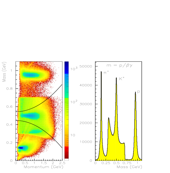
Figure 3: (Color online) Reconstructed mass for positively charged particles. The left figure shows the mass plotted against the measured momentum. The lines show the mass cuts used to identify kaon candidates. A logarithmic yield density scale is employed. The right figure shows the reconstructed mass. These spectra were made from the kaon-filtered data files. The kaon peak is enhanced relative to the pion and proton peaks in the range from 0.3 to 0.7 GeV due to the filtering condition.

Hyperons are identified by using the four-momenta of the electron beam, scattered electron, and the $K^{+}$ candidate. The missing mass distribution contains a background that includes a continuum beneath the hyperons from multi-particle final states with misidentified pions and protons, as well as events from $ep$ elastic scattering (protons misidentified as kaons) and events from $\pi^{+}n$ final states (pions misidentified as kaons). The elastic events are kinematically correlated and show up clearly in plots of $\theta_{K}^{*}$ versus missing mass and $\theta_{K}$ versus $Q^{2}$ (Figs. 4a and b, respectively). A cut on the elastic band in the $\theta_{K}$ (lab angle) versus $Q^{2}$ plot removes them without a significant loss of hyperon yield. The $\pi^{+}n$ events are removed with a simple missing-mass cut in which the detected hadron is assumed to be a pion. The resulting hyperon missing-mass distribution over the entire kinematic range is shown in Fig. 5. Both the $\Lambda(1116)$ and $\Sigma^{0}(1193)$ hyperons are apparent, along with several higher mass hyperons.

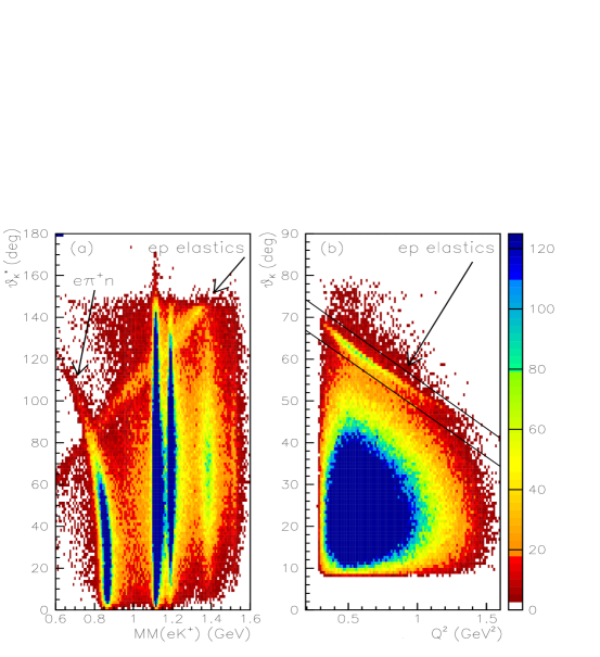
Figure 4: (Color online) (a) $\theta_{K}^{*}$ vs. $p(e,e^{\prime}K^{+})$ missing mass showing $ep$ elastic events and $e^{\prime}\pi^{+}n$ events. The vertical bands correspond to ground state $\Lambda(1116)$ and $\Sigma^{0}(1193)$ hyperons, and the $\Sigma^{0}(1385)/\Lambda(1405)$ hyperons. (b) $\theta_{K}$ (lab angle) vs. $Q^{2}$ for $p(e,e^{\prime}K^{+})$ events showing the $ep$ elastic events and the cut used to remove them.

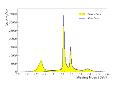
Figure 5: (Color Online) Missing mass for $p(e,e^{\prime}K^{+})$ summed over the entire range of $Q^{2}$, $W$, $\cos\theta_{K}^{*}$, and $\phi$ of the data before and after removing the elastic $ep$ events and the $e^{\prime}\pi^{+}n$ events.

IV.4 Background Corrections

To remove the multi-particle final-state background channels such as $e^{\prime}p\pi\pi$, the phase space background was modeled by selecting the tails of the pion and proton mass distributions. To do this, hadrons in the mass region from 0.275 to 0.725 GeV but outside of the momentum-dependent kaon mass cuts were selected. Background missing mass distributions were calculated for these particles assigning them the kaon mass. These background distributions were fit to the $p(e,e^{\prime}K^{+})$ missing mass distribution using a maximum log likelihood method appropriate for low statistics. The fraction of each background distribution present in the data was thus estimated, and the normalized background contributions were subtracted from the data. Fig. 6 shows the missing mass distributions for two representative bins with the fitted background distributions overlaid. The $\Lambda$ hyperon yields are the number of events in the background-subtracted missing mass spectra in the mass range from 1.095 to 1.165 GeV.

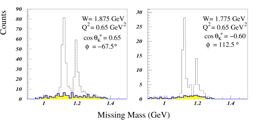
Figure 6: (Color Online) Examples of the background fit results for two typical kinematic bins with $h=+1$. The plots show the raw missing mass plots with the fitted background (solid histogram) overlaid.

IV.5 Detector Efficiency and Acceptance

Geometric fiducial cuts were used in order to ensure that all final state charged particles were detected within the volume of CLAS where the detection efficiency is relatively large and uniform. These cuts remove the edges of the CLAS detectors and depend upon the momentum of the particles, as well as the torus magnetic field setting. The response of the CLAS detector was simulated using GSIM, a GEANT-based geant simulation package for CLAS, that combines the geometrical configuration with the inefficiencies of the various parts of the detector. Monte Carlo techniques were used to generate $p(\vec{e},e^{\prime}K^{+})\Lambda$ events for each helicity state of the incident electrons by including the helicity-dependent fifth structure function in the Mart and Bennhold model mart ; lee .

Acceptance correction factors were obtained for each kinematic bin of $Q^{2}$, $W$, $\cos\theta_{K}^{*}$, and $\phi$, and the two torus field settings, and the effect of the acceptance corrections on the helicity-dependent asymmetries was examined. In the limit of large statistics in the Monte Carlo simulation, the corrected asymmetries are indistinguishable from the uncorrected asymmetries. One should not expect any helicity dependence to the CLAS acceptance outside of negligible bin-migration effects. Thus, the acceptance correction was observed to cancel out (within the statistical uncertainties of both the data and Monte Carlo) in the asymmetry, and no acceptance corrections were applied to the asymmetry measurements. However, a systematic uncertainty associated with not including acceptance corrections has been estimated (see Section IV.8).

IV.6 Radiative Corrections

Radiative corrections were performed on the extracted reaction yields using the exact calculation for the exclusive approach by Afanasev et al. andrei . This approach is based on the covariant procedure of infrared-divergence cancellation by Bardin and Shumeiko Bardin . The exclusive approach is used to correct the cross section, not only in terms of the leptonic variables, but also the hadronic variables in exclusive electroproduction. These calculations were adapted for kaon electroproduction in this work with a cross section model that included a contribution from $\sigma_{LT^{\prime}}$. The radiative correction factors were the ratio of the Born and the radiative cross sections, described in terms of four kinematic variables, $Q^{2}$, $W$, $\cos\theta_{K}^{*}$, and $\phi$. The radiative corrections are up to 30% for a given helicity state but essentially cancel out in the asymmetries.

IV.7 Extraction of $\sigma_{LT^{\prime}}$

The extraction of $\sigma_{LT^{\prime}}$ requires knowledge of both the asymmetry $A_{LT^{\prime}}$ and the unpolarized cross section $\sigma_{0}$, which can be seen by rearranging Eq.(9) as:

$$\frac{A_{LT^{\prime}}\sigma_{0}}{\sqrt{\epsilon(1-\epsilon)}}=\sigma_{LT^{\prime}}\sin\phi.$$ (11)

$A_{LT^{\prime}}$ is determined by forming the asymmetry of the $K^{+}\Lambda$ yields for the positive and negative beam helicity states ($h=\pm$1) as:

$$A_{LT^{\prime}}=\frac{\frac{d\sigma}{d\Omega_{K}^{*}}^{+}-\frac{d\sigma}{d\Omega_{K}^{*}}^{-}}{\frac{d\sigma}{d\Omega_{K}^{*}}^{+}+\frac{d\sigma}{d\Omega_{K}^{*}}^{-}}=\frac{1}{P_{b}}\left(\frac{N^{+}-N^{-}}{N^{+}+N^{-}}\right),$$ (12)

where $\frac{d\sigma}{d\Omega_{K}^{*}}^{\pm}$ is the cross section given by Eq.(7) and $N^{\pm}$ correspond to the corrected yields for the positive and negative helicity states. The electron beam is partially polarized, therefore, the measured asymmetries are also scaled by the measured beam polarization, $P_{b}$.

A correction for the beam charge asymmetry (differences in the integrated beam charge for the different helicity states of the beam) is also included. This is an extremely small correction and was measured to be $2.99\times 10^{-3}$. It was determined by measuring the helicity-dependent yield ratio for $ep$ elastic scattering, which, outside of parity-violating effects, is exactly one.

The unpolarized differential cross sections, ${\sigma}_{0}$, for the $p(e,e^{\prime}K^{+})\Lambda$ reaction that are used in this work, are the published CLAS results from the same data set 5st . The data from Ref. 5st were bin centered in $Q^{2}$, $W$, and $\cos\theta_{K}^{*}$. In that analysis, $\sigma_{0}$ was measured with the same binning in the variables $Q^{2}$, $W$, and $\cos\theta_{K}^{*}$, and the $\phi$-dependent cross sections were then used to extract the structure functions, $\sigma_{U}=\sigma_{T}+\epsilon\sigma_{L}$, $\sigma_{TT}$, and $\sigma_{LT}$.

In order to smooth out the statistical fluctuations of the unpolarized cross section data, a two-dimensional simultaneous fit in $\phi$ and $\cos\theta_{K}^{*}$ of the data has been done. The resulting fitted $\phi$- and $\cos\theta_{K}^{*}$-dependent cross sections have been used in the extraction of $\sigma_{LT^{\prime}}$. The measured $\phi$-dependent cross section in a given bin $\phi^{i}$ is the cross section $\bar{\sigma}^{i}_{0}$ averaged over the span of the $\phi$ bin from $\phi^{i}_{l}$ to $\phi^{i}_{u}$ (upper and lower limits of the bin), and is given by:

$$\bar{\sigma}^{i}_{0} = \frac{1}{\Delta\phi^{i}}\int_{\phi^{i}_{l}}^{\phi^{i}_{u}}\left(\sigma_{U}+c_{+}\sigma_{LT}\cos\phi+\epsilon\sigma_{TT}\cos 2\phi\right)d\phi$$

$$= \frac{1}{\Delta\phi^{i}}\left(\sigma_{U}\Delta\phi^{i}+c_{+}\sigma_{LT}\left(\sin\phi^{i}_{u}-\sin\phi^{i}_{l}\right)+\frac{\epsilon}{2}\sigma_{TT}\left(\sin 2\phi^{i}_{u}-\sin 2\phi^{i}_{l}\right)\right),$$

where $\Delta\phi^{i}=\phi^{i}_{u}-\phi^{i}_{l}$ and $c_{+}=\sqrt{\epsilon(1+\epsilon)}$.

In addition to the trivial $\phi$ dependence, the unpolarized cross section has some unknown $\cos\theta_{K}^{*}$ dependence. It has been assumed that each of the separated structure functions can be described by a third-order polynomial in $x=\cos\theta_{K}^{*}$ as:

$$\sigma_{U} = U_{0}+U_{1}x+U_{2}x^{2}+U_{3}x^{3},$$ (14)

$$c_{+}\sigma_{LT} = LT_{0}+LT_{1}x+LT_{2}x^{2}+LT_{3}x^{3},$$ (15)

$$\epsilon\sigma_{TT} = TT_{0}+TT_{1}x+TT_{2}x^{2}+TT_{3}x^{3}.$$ (16)

Samples of the resulting fits are shown in Fig. 7. In each plot, the black solid line is the best fit and the dashed lines represent a $\pm 1\sigma$ error band extracted from the error matrix of the fit. As expected, the error band is smaller than the uncertainty of the nearby data points. This leads to a smaller contribution to the uncertainty of $\sigma_{LT^{\prime}}$ than if the $\sigma_{0}$ data were used directly. The red/light dashed lines in the figures are from using the one-dimensional $\phi$ fits used in the structure function separation of Ref. 5st . The one-dimensional $\phi$ fits are very similar to the simultaneous $\phi$/$\cos\theta_{K}^{*}$ fits and usually fall within the error band, while the unpolarized structure functions also agree well with those extracted in Ref. 5st . This parameterization of the cross section is then used to determine the $\phi$-dependent cross section averaged over the same bin size as each corresponding asymmetry point.

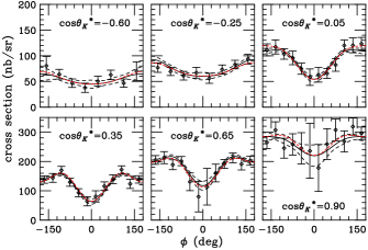
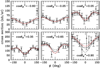
Figure 7: (Color online) Fits to the unpolarized cross section $\sigma_{0}$ vs. $\phi$ for our six $\cos\theta_{K}^{*}$ points for $W$=1.875 GeV and $Q^{2}$=0.65 and 1.00 GeV² (top and bottom panels, respectively). The data and red/light short-dashed curves are from Ref. 5st . The solid black curve in each plot is from the fit described in the text and the dashed curves represent a $\pm 1\sigma$ error band around the fit.

As with the cross sections, the measured asymmetries are the average values over the span of the given $\phi$ bins. Integrating Eq.(9) over the size of the $\phi$ bin results in:

$$A_{LT^{\prime}}=A^{meas}_{LT^{\prime}}\frac{\sin\phi\ \Delta\phi}{\cos\phi_{l}-\cos\phi_{u}}.$$ (17)

The asymmetry $A_{LT^{\prime}}$ has not been corrected for the finite bin size in the variables $Q^{2}$, $W$, and $\cos\theta^{*}_{K}$. As will be discussed in Section IV.8, such corrections are very small compared to the uncertainties, and are very sensitive to the model choice. Therefore, a systematic uncertainty associated with not making this correction has been estimated.

To extract $\sigma_{LT^{\prime}}$, a simple sine fit was performed according to Eq.(11), where the kinematic factor $\sqrt{\epsilon(1-\epsilon)}$ has been calculated at the bin-centered value of $Q^{2}$ and $W$ for each bin (see Table 1). Samples of the data and the resulting fits are shown in Fig. 8. The solid curves are the fit result and the dashed curves indicate the $\pm 1\sigma$ error band from the fit.

The error bars on the data points are a combination of the contributions from both $A_{LT^{\prime}}$ and $\sigma_{0}$, and are given by:

$$\delta(A_{LT^{\prime}}\sigma_{0})=\sqrt{{(A_{LT^{\prime}}\delta\sigma_{0})}^{2}+{(\sigma_{0}\delta A_{LT^{\prime}})}^{2}}.$$ (18)

The uncertainty $\delta A_{LT^{\prime}}$ is the quadrature sum of the statistical and $\phi$-dependent systematic uncertainties (see Section IV.8 for details), while $\delta\sigma_{0}$ comes from the fit of the cross sections described above.

Figure 8: Measured asymmetries multiplied by the unpolarized cross section and divided by the kinematic factor $c_{-}=\sqrt{\epsilon(1-\epsilon)}$ vs. $\phi$ for our six $\cos\theta_{K}^{*}$ points for a typical kinematic bin of $W$=1.875 GeV and $Q^{2}$=0.65 and 1.00 GeV² (top and bottom panels, respectively). The solid curves show the results of the $\sin\phi$ fits and the dashed lines show the $\pm$1$\sigma$ error band from the fits.

IV.8 Systematic Uncertainties

Various sources of systematic uncertainty that affect the measured asymmetries $A_{LT^{\prime}}$ and the extracted structure functions $\sigma_{LT^{\prime}}$ are considered in this analysis. The sources of systematic uncertainty that affect the measured asymmetries include uncertainties due to yield extraction, fiducial cuts, acceptance corrections, radiative corrections, and the beam charge asymmetry. These are uncorrelated point-to-point uncertainties. Scale-type uncertainties affect $\sigma_{LT^{\prime}}$ only and include the bin centering and beam polarization uncertainties, as well as the systematic uncertainties in the measurement of the unpolarized cross section, $\sigma_{0}$. Table 2 summarizes the various systematic uncertainties that affect $A_{LT^{\prime}}$ and $\sigma_{LT^{\prime}}$.

In the case of the $\phi$-dependent uncertainties, all but the yield extraction uncertainty are dominated by statistical uncertainties. The uncertainty due to the background-subtraction (yield extraction) procedure was estimated to be the same as was determined in the cross section extraction procedure 5st . In that analysis, various changes to the procedures were studied, such as changing the histogram bin size in the fitting procedure and using different forms for the background shape (e.g. using both misidentified pions and protons, only misidentified pions, and only misidentified protons), and it was concluded that all systematic effects get larger in direct proportion to the size of the statistical uncertainty. When statistics are good (roughly 100 counts/bin), the residual systematic uncertainties are very small. It has been determined that the remaining systematic uncertainty due to the yield extraction is roughly equal to 25$\%$ of the size of the statistical uncertainty in any given bin (defined by $Q^{2}$, $W$, and $\cos\theta_{K}^{*}$). This uncertainty was added linearly to the statistical uncertainty for the helicity-dependent yields (i.e. the overall statistical uncertainty was increased on each yield by a factor of 1.25).

In order to estimate the uncertainties due to the fiducial cuts, acceptance, and radiative corrections, the corrected or nominal asymmetries were compared to the asymmetries that resulted from using either an alternative correction or cut. The RMS width of the difference between the nominal and alternative asymmetries, weighted by the statistical uncertainty of the asymmetry, was determined, and this was used as the estimate of the systematic uncertainty. For the acceptance effect, the difference between using no acceptance correction (nominal) and applying an acceptance correction was studied. This is certainly an overestimate in this case, however, the uncertainty is small compared to the other sources of systematic uncertainty and much smaller than the statistical uncertainty. For the fiducial cut uncertainty, the extent of the fiducial cuts was varied over a large range. The resulting asymmetries were compared to the nominal asymmetries. Finally, for the radiative correction uncertainty, two different models were used as input to the radiative correction code. It has been implicitly assumed that the correction method is dominated by model uncertainties.

The uncertainties for the background subtraction, fiducial cuts, acceptance, radiative corrections, and beam charge asymmetry, are absolute uncertainties and were added in quadrature to the statistical uncertainty of each asymmetry data point before the extraction of $\sigma_{LT^{\prime}}$.

Type	Source	Systematic Uncertainty $A_{LT^{\prime}}$
$A_{LT^{\prime}}$	Yield Extraction Method	0.25$\times$stat. uncertainty of yield
$\phi$ dependent	Acceptance Function (GSIM)	$0.033$
	Fiducial Cuts	$0.027$
	Radiative Corrections	$0.009$
	Beam Charge Asymmetry	$1.45\times 10^{-4}$
$\sigma_{LT^{\prime}}$	Bin Centering	5.8 nb/sr (absolute)
	Beam Polarization	$\frac{\delta P_{b}}{P_{b}}\sigma_{LT^{\prime}}=0.023\sigma_{LT^{\prime}}$
	Unpolarized Cross Section	$0.124\ \sigma_{LT^{\prime}}$, $0.115\ \sigma_{LT^{\prime}}$

Table 2: Summary of the systematic uncertainties applied to $A_{LT^{\prime}}$ and $\sigma_{LT^{\prime}}$. The two entries for the unpolarized cross section uncertainty are for the $Q^{2}=$0.65 and 1.00 GeV² data sets.

The end result of this analysis is the extraction of the fifth structure function, $\sigma_{LT^{\prime}}$, at specific points in $Q^{2}$, $W$, and $\cos\theta_{K}^{*}$ using Eq.(11). These kinematic points are listed in Table 1 (note that our bin “center” for the $Q^{2}$ bin from 0.8 to 1.3 GeV² was 1.00 GeV² as given by Ref. 5st , and not the true center at $Q^{2}$=1.05 GeV²). The beam-helicity asymmetry, however, is sorted into particular bins of $Q^{2}$, $W$, and $\cos\theta_{K}^{*}$, and thus a bin-centering correction must be considered to extract $\sigma_{LT^{\prime}}$ at specific kinematic points. The bin-centering correction would be applied to the binned asymmetries as:

$$A_{LT^{\prime}}^{BC}=A_{LT^{\prime}}\left(\frac{A_{LT^{\prime}}^{point}}{A_{LT^{\prime}}^{avg}}\right)_{model}=A_{LT^{\prime}}\cdot BC,$$ (19)

where $A_{LT^{\prime}}^{BC}$ represents the bin-centered beam-helicity asymmetry and $A_{LT^{\prime}}$ represents the bin-averaged asymmetry. To determine the bin-centering correction factors $BC$ for this analysis, a model of the CLAS acceptance in $Q^{2}$ vs. $W$ was developed to account for the partially filled bins. The $BC$ factors necessarily rely on a model of $A_{LT^{\prime}}$, where $A_{LT^{\prime}}^{point}$ is the asymmetry calculated at a specific kinematic point ($Q^{2}$, $W$, $\cos\theta_{K}^{*}$, $\phi$) and $A_{LT^{\prime}}^{avg}$ is the calculated bin-averaged asymmetry. The $BC$ factors were determined using the hadrodynamic model of Mart and Bennhold mart as a starting point. Within the framework of this model, several different choices of elementary reaction models are available with different ingredients, such as the resonant amplitudes included, as well as the functional forms for the meson and baryon form factors, i.e. the $K^{+}$ form factor, the $K^{+}K^{*+}\gamma$ transition form factor, and the $\Lambda$ magnetic form factor. The differences between the structure functions derived using the different models for the bin-centering corrections on the asymmetries are quite small and none is clearly preferred by the asymmetry data. The assigned systematic uncertainty associated with the bin-centering corrections was chosen to be the largest RMS width of the $\sigma_{LT^{\prime}}$ differences using the different models.

The relative systematic uncertainty due to the beam polarization measurement for the data sets used in this analysis is estimated to be $\frac{\delta P}{P}=0.023$. The estimated uncertainty on $\sigma_{LT^{\prime}}$ due to the systematic uncertainty on the beam polarization is given by:

$$\delta\sigma_{LT^{\prime}}=|A_{LT^{\prime}}^{meas}|\frac{\delta P_{b}}{P_{b}^{2}}=|\sigma_{LT^{\prime}}|\frac{\delta P_{b}}{P_{b}}.$$ (20)

The resulting values of $\sigma_{LT^{\prime}}$ also have an additional uncertainty associated with the systematic uncertainty in the measurement of the unpolarized cross section, $\sigma_{0}$. The estimated systematic uncertainties for the cross sections are given in Ref. 5st , which result in corresponding systematic uncertainties of 0.124$\sigma_{LT^{\prime}}$ and 0.115$\sigma_{LT^{\prime}}$ for $Q^{2}$ = 0.65 and 1.00 GeV², respectively. The quadrature sum of the uncertainties due to the bin-centering correction, beam polarization, and unpolarized cross section, are shown by the shaded bars on the results (see Section V, Figs. 9 to 12).

V Results and Discussions

The angular dependence of $\sigma_{LT^{\prime}}$ for various $W$ points for the two $Q^{2}$ points is shown in Figs. 9 and 10, along with comparisons to several model calculations. The lower $Q^{2}$ data shown in Fig. 9 is rather flat over the full range of energy and angle, with no strong structures visible. Unlike the low $Q^{2}$ data, a strong $W$ and angular dependence is observed in the higher $Q^{2}$ data (Fig. 10). The angular dependence shows an interesting peaking at middle angles for the lowest $W$ point ($W$=1.65 GeV), while a rapid sign change is seen at both $W$= 1.875 and 1.925 GeV at central angles.

The extracted $\sigma_{LT^{\prime}}$ structure function results are shown as a function of $W$ for various $\cos\theta_{K}^{*}$ points for the $Q^{2}$ points at 0.65 and 1.00 GeV² in the top panels of Figs. 11 and 12, respectively. For the lower $Q^{2}$ data, Fig. 11 shows that for the four backward-most kaon center-of-mass scattering angles ($\cos\theta_{K}^{*}$=-0.60, -0.25, 0.05, and 0.35), $\sigma_{LT^{\prime}}$ exhibits a smooth energy dependence with a fall off of the structure function to zero at the highest $W$ points. In the forward kaon scattering angles, $\cos\theta_{K}^{*}$=0.65 and 0.90, where the reaction is expected to be dominated by $t$-channel exchange, $\sigma_{LT^{\prime}}$ is consistent with zero to within the rather large error bars of the data, and no obvious structures are present. This might indicate the dominance of a single $t$-channel exchange.

For the higher $Q^{2}$ data (see Fig. 12), the range of $W$ is limited by the CLAS acceptance. Here the $W$ dependence of $\sigma_{LT^{\prime}}$ is similar to the lower $Q^{2}$ data at the more forward angles, $\cos\theta_{K}^{*}$=0.65 and 0.90. However, there is a notable feature in the $W$ dependence in the backward and middle kaon angles. At $\cos\theta_{K}^{*}$=-0.25, 0.05 and 0.35, the data show an interesting interference feature around 1.9 GeV, with a rapid change of sign at $\cos\theta_{K}^{*}$=0.05 and 0.35. While at the very backward angles, $\cos\theta_{K}^{*}$=-0.60, a strong enhancement is seen at about $W$=1.7 GeV with a flat response for higher $W$. For both of the $Q^{2}$ values, $\sigma_{LT^{\prime}}$ goes to zero at higher $W$.

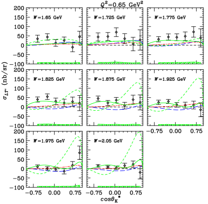
Figure 9: (Color online) Polarized structure function $\sigma_{LT^{\prime}}$ (nb/sr) vs. $\cos\theta_{K}^{*}$ for $Q^{2}$=0.65 GeV² and $W$ points as indicated. The curves are calculations from the MB isobar model mart_code (blue long dashes), the GLV Regge model guidal_code (red dash-dot), the Ghent RPR model including a $D_{13}(1900)$ state ghent_code (green solid), and the Ghent RPR model including a $P_{11}(1900)$ state ghent_code (green short dashes). The shaded bars indicate the estimated overall systematic uncertainty on the results.

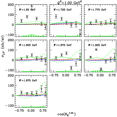
Figure 10: (Color online) Polarized structure function $\sigma_{LT^{\prime}}$ (nb/sr) vs. $\cos\theta_{K}^{*}$ for $Q^{2}$=1.00 GeV² and $W$ bins as indicated. The curves are as indicated in Fig. 9.

The results are compared with calculations from the MB isobar model mart_code (blue long dashes), the GLV Regge model guidal_code (red dash-dot), the Ghent RPR model ghent_code including a $D_{13}(1900)$ state (green solid), and the Ghent RPR model ghent_code including a $P_{11}(1900)$ state (green short dashes). In general, none of the available models fully describes these data over the $Q^{2}$, $W$, and $\cos\theta_{K}^{*}$ ranges measured. The MB and GLV models under predict the strength of $\sigma_{LT^{\prime}}$, although they qualitatively follow the trends of the data. From the comparisons, the RPR model including the $P_{11}(1900)$ state is clearly ruled out as already indicated in Ref. ghent , but the RPR model including the $D_{13}(1900)$ state seems to best describe the data qualitatively. However, each of these models misses key features of the data. The disagreements with the isobar models (MB and RPR) may not be too surprising as they have not been fit to these data. Therefore, the $\sigma_{LT^{\prime}}$ structure function provides for additional new constraints on the model parameters.

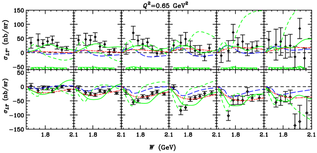
Figure 11: (Color online) Polarized structure function $\sigma_{LT^{\prime}}$ as a function of $W$ for various $\cos\theta_{K}^{*}$ (upper panel) compared to the measured $\sigma_{LT}$ from Ref. 5st (lower panel) for $Q^{2}$=0.65 GeV². Plots are shown for $\cos\theta^{*}_{K}$=-0.60, -0.25, 0.05, 0.35, 0.65, and 0.90 (left to right). The curves are as indicated in Fig. 9.

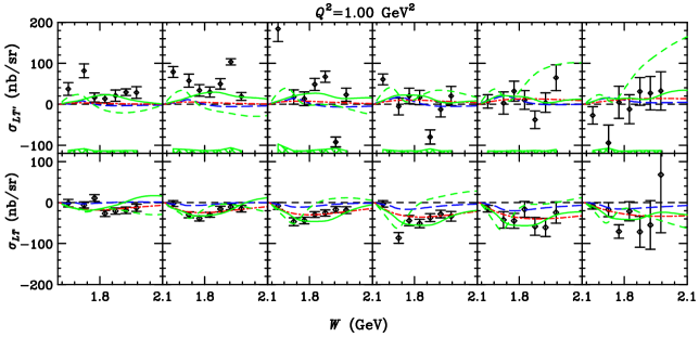
Figure 12: (Color online) Polarized structure function $\sigma_{LT^{\prime}}$ as a function of $W$ for various $\cos\theta_{K}^{*}$ (upper panel) compared to the measured $\sigma_{LT}$ from Ref. 5st (lower panel) for $Q^{2}$=1.00 GeV². Plots are shown for $\cos\theta^{*}_{K}$=-0.60, -0.25, 0.05, 0.35, 0.65, and 0.90 (left to right). The curves are as indicated in Fig. 9.

A direct comparison of the measured polarized structure function $\sigma_{LT^{\prime}}$ with $\sigma_{LT}$ from Ref. 5st can reveal some interesting features of the data. This is shown in Figs. 11 and 12 where the polarized structure function $\sigma_{LT^{\prime}}$ is plotted as a function of $W$ for various $\cos\theta_{K}^{*}$ bins and compared with $\sigma_{LT}$ at the same kinematic points. The magnitudes of the two structure functions are comparable in both the lower and higher $Q^{2}$ data, although $\sigma_{LT^{\prime}}$ has larger uncertainties. In the lower $Q^{2}$ data at the most backward kaon center-of-mass angle, $\cos\theta_{K}^{*}$=-0.60, $\sigma_{LT}$ is essentially zero, while $\sigma_{LT^{\prime}}$ is clearly non-zero. At $\cos\theta_{K}^{*}$=-0.25, 0.05, and 0.35, $\sigma_{LT}$ is similar in shape and magnitude to $\sigma_{LT^{\prime}}$, but with an opposite sign. At the very forward kaon center-of-mass angles, $\cos\theta_{K}^{*}$=0.65 and 0.90, $\sigma_{LT^{\prime}}$ is consistent with zero, while $\sigma_{LT}$ is non-zero. In the higher $Q^{2}$ data, and for backward and middle kaon scattering angles, $\sigma_{LT^{\prime}}$ has some significant deviations from a smooth behavior, indicating significant interferences. However, the shapes of $\sigma_{LT^{\prime}}$ and $\sigma_{LT}$ are quite different.

All of the data included in this work have been entered into the CLAS physics database database .

VI Conclusions

The first measurements of the structure function $\sigma_{LT^{\prime}}$ for $K^{+}\Lambda$ electroproduction have been reported. The data span a range in $W$ from threshold to 2.05 GeV for two $Q^{2}$ points at 0.65 and 1.00 GeV², and span nearly the full center-of-mass angular range of the final state $K^{+}$. In this analysis, the energy and angular dependence of $\sigma_{LT^{\prime}}$ have been investigated. $\sigma_{LT^{\prime}}$ is found to be comparable in size to the unpolarized cross sections. The structure function is surprisingly featureless with energy and angle for the lower $Q^{2}$ data, while the higher $Q^{2}$ data indicate rather strong interference affects near threshold and at $W$ of 1.9 GeV for central angles. $\sigma_{LT^{\prime}}$ is consistent with zero at more forward angles and at higher values of $W$.

The data have been compared with several different model calculations. The GLV Regge calculation generally under predicts the data. This is perhaps not too surprising given that it includes no explicit $s$-channel processes, which are expected to show clear signatures in $\sigma_{LT^{\prime}}$. Comparisons to the MB isobar model and RPR hybrid isobar/Regge model (which did not include any CLAS electroproduction data in their fits) indicate that the model parameters need to be tuned in order to reproduce the overall average strength seen in $\sigma_{LT^{\prime}}$. A bigger challenge for these models is to explain the strong interference signatures in the data. Even though the CLAS $\sigma_{LT}$ and $\sigma_{LT^{\prime}}$ data have rather sizable statistical uncertainties, the data do have a good deal of discriminating power with regard to certain assumptions about which resonant states are included.

The $\sigma_{LT^{\prime}}$ results were also compared with the results of the measurements for $\sigma_{LT}$ 5st at the same kinematic points. While $\sigma_{LT^{\prime}}$ has larger uncertainties, the magnitudes of the two structure functions are comparable. In our lower $Q^{2}$ data, $\sigma_{LT^{\prime}}$ is quite smooth with $W$ and $\cos\theta_{K}^{*}$. However, at the high $Q^{2}$ value, $\sigma_{LT^{\prime}}$ shows strong interference and/or FSI signatures at middle and backward kaon scattering angles. Together, these two observables provide more complete information on the amplitudes underlying the longitudinal-transverse response for this reaction.

The question of the presence of any new resonances must wait for further work with the existing hadrodynamic models and partial wave analyses applied to the full range of the data. Fortunately, the new information presented here will impose reasonable constraints on the amplitudes used to describe electroproduction of $K^{+}\Lambda$ and $K^{+}\Sigma^{0}$ final states, making these models more reliable for future interpretation and prediction.

References

- (1) R. Koniuk and N. Isgur, Phys. Rev. D 21, 1868 (1980).
- (2) S. Capstick and W. Roberts, Phys. Rev. D 47, 1994 (1993).
- (3) S. Capstick and W. Roberts, Phys. Rev. D 49, 4570 (1994).
- (4) S. Capstick and W. Roberts, Phys. Rev. D 58, 074011 (1998).
- (5) P. Ambrozewicz et al. (CLAS Collaboration), Phys. Rev. C 75, 045203 (2007).
- (6) G. Niculescu et al., Phys. Rev. Lett. 81, 1805 (1998).
- (7) R.M. Mohring et al., Phys. Rev. C 67, 055205 (2003).
- (8) D.S. Carman et al. (CLAS Collaboration), Phys. Rev. Lett. 90, 131804 (2003).
- (9) Brian A. Raue and Daniel S. Carman, Phys. Rev. C 71, 065209 (2005).
- (10) C. N. Brown et al., Phys. Rev. Lett. 28, 1086 (1972).
- (11) C.J. Bebek et al., Phys. Rev. Lett. 32, 21 (1974).
- (12) T. Azemoon et al., Nucl. Phys. B 95, 77 (1975).
- (13) C.J. Bebek et al., Phys. Rev. D 15, 594 (1977); C.J. Bebek et al., Phys. Rev. D 15, 3082 (1977).
- (14) P. Brauel et al., Z. Phys. C 3, 101 (1979).
- (15) M.Q. Tran et al., Phys. Lett. B 445, 20 (1998).
- (16) K.H. Glander et al., Eur. Phys. J. A 19, 251 (2004).
- (17) J.W.C. McNabb et al. (CLAS Collaboration), Phys. Rev. C 69, 042201(R) (2004).
- (18) R. Bradford et al. (CLAS Collaboration), Phys. Rev. C 73, 035202 (2006).
- (19) R. Bradford et al. (CLAS Collaboration), Phys. Rev. C 75, 035205 (2007).
- (20) R.G.T. Zegers et al., Phys. Rev. Lett. 91, 092001 (2003).
- (21) M. Sumihama et al., Phys. Rev. C 73, 035214 (2006).
- (22) C. Bennhold, H. Haberzettl, and T. Mart, Proceedings of Perspectives in Hadronic Physics, edited by S. Boffi et al., Singapore, World Scientific, 2000.
- (23) T. Mart and C. Bennhold, Phys. Rev. C 61, 012201 (2000); H. Haberzettl et al., Phys. Rev. C 58, R40 (1998).
- (24) B. Saghai, proceedings of Hadrons and Nuclei conference, edited by I. Cheon et al., AIP Conference Proceedings 594, 421 (2001).
- (25) T. Corthals et al., preprint arXiv:0704.3691, submitted for publication (2007); T. Corthals et al., Phys. Rev. C 75, 045204 (2007).
- (26) C.W. Akerlof, W.W. Ash, K. Berkelman, and C.A. Lichtenstein, Phys. Rev. 163, 1482 (1967).
- (27) G. Knochlein, D. Drechsel, and L. Taitor, Z. Phys. A 352, 327 (1995).
- (28) S. Boffi, C. Guisti, and F.D. Pacati, Phys. Rep. 226, 1 (1993); S. Boffi, C. Guisti, and F.D. Pacati, Nucl. Phys. A 435, 697 (1985).
- (29) Some authors use a pre-factor for the term of , for the () term of () instead, where parameterizes the longitudinal polarization of the virtual photon. Some also take a () term out of the definition of () and a term out of the definition of (see e.g. Ref. zeit ).
- (30) B. Julia-Diaz et al., Phys. Rev. C 73, 055204 (2006).
- (31) W.T. Chiang et al., Phys. Rev. C 69, 065208 (2004).
- (32) V. Shklyar, H. Lenske, and U. Mosel, Phys. Rev. C 72, 015210 (2005).
- (33) T.-S.H. Lee and L.C. Smith, J. Phys. G 34, S83 (2007).
- (34) A.V. Sarantsev et al., Eur. Phys. J. A 25, 441 (2005).
- (35) A. Anisovich et al., Eur. Phys. J. A 24, 111 (2005); A. Anisovich et al., Eur. Phys. J. A 25, 427 (2005).
- (36) F. X. Lee, T. Mart, C. Bennhold, H. Haberzettl, and L.E. Wright, Nucl. Phys. A 695, 237 (2001).
- (37) M. Guidal, J.-M. Laget, and M. Vanderhaghen, Nucl. Phys. A 627, 645 (1997); Phys. Rev. C 61, 025204 (2000); Phys. Rev. C 68, 058201 (2003).
- (38) B.A. Mecking et al., Nucl. Inst. and Meth. A 503, 513 (2003).
- (39) M.D. Mestayer et al., Nucl. Inst. and Meth. A 449, 81 (2000).
- (40) E.S. Smith et al., Nucl. Inst. and Meth. A 432, 265 (1999).
- (41) G. Adams et al., Nucl. Inst. and Meth. A A465, 414 (2001).
- (42) M. Amarian et al., Nucl. Inst. and Meth. A 460, 239 (2001).
- (43) R. Brun et al., CERN-DD-78-2-REV, (1978).
- (44) A. Afanasev, I. Akushevich, V. Burkert, and K. Joo, Phys. Rev. D 66, 074004 (2002).
- (45) D.Y. Bardin and N.M. Shumeiko, Nucl. Phys. B 127, 242 (1977).
- (46) T. Mart, code from private communication.
- (47) M. Guidal, code from private communication.
- (48) T. Corthals, calculations from private communication.
- (49) CLAS physics database, http://clasweb.jlab.org/physicsdb.