Phenomenological analysis of quantum collapse as source of the seeds of cosmic structure
Abstract
The standard inflationary version of the origin of the cosmic structure as the result of the quantum fluctuations during the early universe is less than fully satisfactory as has been argued in [A. Perez, H. Sahlmann, and D. Sudarsky, Class. Quantum Grav., 23, 2317, (2006)]. A proposal is made there of a way to address the shortcomings by invoking a process similar to the collapse of the quantum mechanical wave function of the various modes of the inflaton field. This in turn was inspired on the ideas of R. Penrose about the role that quantum gravity might play in bringing about such breakdown of the standard unitary evolution of quantum mechanics. In this paper we study in some detail the two schemes of collapse considered in the original work together with an alternative scheme, which can be considered as “more natural” than the former two. The new scheme, assumes that the collapse follows the correlations indicated in the Wigner functional of the initial state. We end with considerations regarding the degree to which the various schemes can be expected to produce a spectrum that resembles the observed one.
pacs:
98.30.Bp, 98.80.Cq, 03.65.TaI Introduction
In recent years, there have been spectacular advances in physical cosmology, resulting from remarkable increase in the accuracy of the observational techniques and exemplified by the Supernova Surveys Supernovas , the studies of large scale structure Structure and the highly accurate observations from various recent studies in particular those of Wilkinson Microwave Anisotropy Probe (WMAP) wmap2007 . These observations have strengthened the theoretical status of the Inflationary scenarios among cosmologists.
We should note however that while much of the focus of the research in Inflation has been directed towards the elucidation of the exact form of the inflationary model (i.e. the number of fields, the form of the potential, and the occurrence of non-minimal couplings to gravity to name a few), much less attention has been given to the questions of principle, as how the initial conditions are determined, what accounts for the low entropy of the initial state, and how exactly does the universe transit from a homogeneous and isotropic stage to one where the quantum uncertainties become actual inhomogeneous fluctuations. There are of course several works in which this issues are addressed Other , Others but as explained in Perez2006 , Sudarsky06b , Sudarsky07 the fully satisfactory account of the last of them seems to require something beyond the current understanding of the laws of physics. The point is that the predictions of inflation in this regard can not be fully justified in any known and satisfactory interpretational scheme for quantum physics. The Copenhagen interpretation, for instance, is inapplicable in that case, due to the fact that we, the observers, are part of the system, and to make things even worse we are in fact part of the outcome of the process we wish to understand, Galaxies, Stars, planets and living creatures being impossible in a homogeneous and isotropic universe 111Further issues about the identification of ensemble averages with time averages, which are valid under the ergodic hypothesis can be raised in the cosmological context where assumptions of ergodicity and equilibrium seem to be much less justified.. The arguments and counter-arguments that have arisen in regard to this aspect of the article mentioned above have been discussed in various other places by now and we point the reader who is interested in that debate to that literature debate , Sudarsky07 . In the present work we will focus on a more detailed study of the collapse schemes and on the traces they might leave on the observational data. Nevertheless, and in order to make the article self contained, we will briefly review the motivation and line of approach described in detail in Perez2006 .
To clarify where lies the problem, and the way in which it is addressed in Perez2006 we will review in a nutshell, the standard explanation of the origin of the seeds of cosmic structure in the Inflationary paradigm:
-
•
One starts with an homogeneous and isotropic spacetime222Inflation could work if we don’t start -strictly- with this condition, but after some e-foldings the universe reaches this stage. The inflaton field is the dominant matter in this spacetime, and it is in its vacuum quantum state, which is homogeneous and isotropic too. The field is in fact described in terms of its expectation value represented as a scalar field which depends only on cosmic time but not on the spatial coordinates, and a quantum or “fluctuating part” which is in the adiabatic vacuum state, which is an homogeneous and isotropic state (something that can be easily verified by applying the generators of rotations or translations to the state).
-
•
The quantum “fluctuations” of the inflaton acts as perturbations 333 We find this wording unfortunate because it leads people to think that something is fluctuating in the sense of Brownian motion, while a wording such as ”quantum uncertainties” would evoke something like the wave packet associated with a ground state of an harmonic oscillator which is a closer analogy with what we have at hand. of the inflaton field and through the Einstein Field Equations (EFE) as perturbations of the metric.
-
•
As inflation continues the physical wave length of the various modes of the inflaton field become larger than the Hubble Radius (Horizon-crossing as referred commonly in the literature), and the quantum amplitudes of the modes freeze. At that moment one starts regarding such modes as actual waves of in a classical field. Later on, after inflation ends, and as the Hubble Radius grows, the fluctuations “re-enter the Horizon”, transforming at that point into the seeds of the cosmic structure.
The last step is usually refereed as the quantum to classical transition. There are of course several schools of though about the way one must consider such transition: from those using the established physical paradigms Other , Others , to views advocating a certain generalization of the standard formalismsHartle . The two works Other , Hartle focus concretely in a full blown quantum cosmology, and its interpretational problems, which are even more severe than the ones we are dealing with here. In Perez2006 it was argued that such schemes are insufficient, in particular if one expects cosmology to provide a time evolution account starting from the totally symmetric state to an inhomogeneous and anisotropic Universe in which creatures such as humans might eventually arise.
The view taken in Perez2006 (and in this work) intends to be faithful to the notion that physics is always quantum mechanical, and that the only role for a classical description is that of an approximation where the uncertainties in the state of the system are negligibly small and one can take the expectation values as fair description of the aspects of the state one is interested on. However one must keep in mind that behind any classical approximation there should always lie a full quantum description, and thus one should reject any scheme in which the classical description of the universe is inhomogeneous and anisotropic but in which the quantum mechanical description persists in associating to the universe an homogeneous and isotropic state at all times. Thus in Perez2006 , one introduces a new ingredient to the inflationary account of the origin of the seeds of cosmic structure: the self induced collapse hypothesis. I.e. one considers a specific scheme by which a self induced collapse of the wave function is taken as the mechanism by which inhomogeneities and anisotropies arise in each particular scale. This work was inspired in early ideas by Penrose Penrose which regard that the collapse of the wave function as an actual physical process (instead of just an artifact of our description of physics) and which is assumed to be caused somehow by quantum aspects of gravitation. We will not recapitulate the motivations and discussion of the original proposal and instead refer to the reader to the above mentioned works.
The way we treat the transition of our system from a state that is homogeneous and isotropic to one that is not, is to assume that at certain cosmic time, something induces a jump in a state describing a particular mode of the quantum field, in a manner that would be similar to the standard quantum mechanical collapse of the wave function associated with a measurement, but with the difference that in our scheme no external measuring device or observer is called upon as “triggering” that jump (it is worthwhile recalling that nothing of that sort exist, in the situation at hand, to play such role).
The main aim of this article is to compare the results that emerge from the collapse schemes considered in Perez2006 with an alternative scheme of collapse that can be said to more natural than the previous two. In this new scheme 444As we will show, the relevant quantities that one is interested in computing are determined once one characterizes the time of collapse and describes the state after the collapse in terms of the expectation values of the field and momentum conjugate variables. we take into account the correlations in the quantum state of the system before the collapse for the values of field and conjugate momentum variables as indicated by the Wigner functional analysis of the pre-collapse state.
This article is organized as follows: In the Section II we review the formalism used in analysing the collapse process. Section III review how to obtain the wave function for the field from its Fock space description, which is then used in evaluating the Wigner function for the state, and the state that results after the collapse. Section IV describes the details of the spectrum of cosmic fluctuations, resulting from such collapse, and finally, in Section V we discuss these results and those of other collapse schemes vis a vie the empirical data.
II The Formalism
The starting point is the action of a scalar field with minimal coupling to the gravity sector:
| (1) |
One splits the corresponding fields into their homogeneous (“background”) part and the perturbations (“fluctuation”), so the metric and the scalar field are written as : and . With the appropriate choice of gauge (conformal Newton gauge) and ignoring the vector and tensor part of the metric perturbations, the space-time metric is described by.
| (2) |
where is called the Newtonian potential. One then considers the EFEs to zeroth and first order. The zeroth order gives rise the standard solutions in the inflationary stage, where , with with the scalar potential, in slow-regime so ; and the first order EFE reduce to an equation relating the gravitational perturbation and the perturbation of the field
| (3) |
with . The next step involves quantazing the fluctuating part of inflaton field. In fact it is convenient to work with the rescaled field . In order to avoid infrared problems we consider restriction of the system to a box of side , where we impose, as usual, periodic boundary conditions. We thus write the fields as
| (4) |
where is the canonical momentum of the scaled field. The wave vectors satisfy with , and , and . The functions reflect our election of the vacuum state, the so called Bunch-Davies vacuum:
| (5) |
The vacuum state is defined by the condition for all , and is homogeneous and isotropic at all scales. As indicated before, according to the proposal, the self-induced collapse operates in close analogy with a “measurement” in the quantum-mechanical sense, and assumes that at a certain time the part of the state that describes the mode jumps to an new state, which is no longer homogeneous and isotropic. To proceed to the detailed description of this process, one decomposes the fields into their hermitian parts as follows , and .
We note that the vacuum state is characterized in part by the following: its expectation values and its uncertainties are and .
For an arbitrarily given state of the field , we introduce the quantity so that,
| (6) |
which shows that it specifies the main quantity of interest in characterizing the state of the field.
It is convenient for future use to define the following phases, and , keeping in mind that they depend on the conformal time .
The analysis now calls for the specification of the scheme of collapse determining the state of the field after the collapse555 At this point, in fact, all we require is the specification of the expectation values of certain operators in this new quantum state. , which is the main purpose of the next section. With such collapse scheme at hand one then proceeds to evaluate the perturbed metric using a semi-classical description of gravitation in interaction with quantum fields as reflected in the semi-classical EFE’s: . To lowest order this set of equations reduces to
| (7) |
where is the expectation value of the momentum field on the state characterizing the quantum part of the inflaton field. It is worthwhile emphasizing that before the collapse has occurred there are not metric perturbations666This might seem awkward to some readers. It is worth then emphasizing that our view is that, in contrast with what happens with other fields, the fundamental degrees of freedom of gravitation are not related to the metric degrees of freedom in any simple way, but instead the latter appear as effective degrees of freedom of a non-quantum effective theory. Therefore, the quantum uncertainties (we feel ”uncertainties” is a more appropriate word than ”fluctuations”, as the latter suggest that something is actually changing constantly in a random way) associated with the gravitational degrees of freedom are most naturally thought as not having a metric description (as occurs for instance in the Loop Quantum Gravity program where the fundamental degrees of freedom are holonomies and fluxes), and thus that the metric can appear only at the classical level of description, where it satisfies something close to the semiclassical Einstein equation. In other words, from our point of view, it would be incorrect to think of the quantum uncertainties of the metric as appropriate description of the quantum aspects of gravitation, and much less, as satisfying Einstein’s equations. From our point of view, this would be analogous to imagining the quantum indeterminacies associated with the ground state of the hydrogen atom, as described in terms a perturbation of the orbit of an electron in Hydrogen atom, and satisfying Keppler’s equations for the classical Coulomb potential. For more details about these point of view see Perez2006 , Sudarsky06b , Sudarsky07 . The reader should be aware that this is not a view shared by most cosmologists., i.e. the r.h.s. of the last equation is zero, so, it is only after the collapse that the gravitational perturbations appear, i.e. the collapse of each mode represents the onset of the inhomogeneity and anisotropy at the scale represented by the mode. Another point we must stress is that, after the collapse,and in fact at all times, our Universe would be defined by a single state , and not by an ensemble of states. The statistical aspects arise once we note that we do not measure directly and separately each the modes with specific values of , but rather the aggregate contribution of all such modes to the spherical harmonic decomposition of the temperature fluctuations of the celestial sphere (see below).
To make contact with the observations we note that the quantity that is experimentally measured (for instance by WMAP) is , which is expressed in terms of its spherical harmonic decomposition . The contact with the theoretical calculations is made trough the theoretical estimation most likely value of the ’s, which are expressed in terms of the Newtonian potential on the 2-sphere corresponding to the intersection of our past light cone with the of last scattering surface (LSS): , . We must then consider the expression for the Newtonian Potential (7) at those points:
| (8) |
where we have introduced the factor to represent the physics effects of the period between reheating and decoupling.
Writing the coordinates of the points of interest on the surface of last scattering as , where is the comoving radius of that surface and are the standard spherical coordinates of the sphere, and using standard results connecting Fourier and spherical expansions we obtain
| (9) | ||||
| (10) |
As indicated above statistical considerations arise when noting that the equation (8) indicates that the quantity of interest is in fact the result of a large number (actually infinite) of harmonic oscillator each one contributing with a complex number to the sum, leading to what is in effect a two dimensional random walk whose total displacement corresponds to the observational quantity. Note that this part of the analysis is substantially different from the corresponding one in the standard approach. In order to obtain a prediction, we need to find the most likely value of the magnitude of such total displacement.
Thus we must concern ourselves with:
| (11) |
and to obtain the “most likely” value for this quantity. This we do with the help of the imaginary ensemble of universes777This is just a mathematical evaluation device and no assumption regarding the existence of such ensemble of universes is made or needed. These aspects of our discussion can be regarded as related to the so called cosmic variance problem. and the identification of the most likely value with the ensemble mean value.
As we will see, the ensemble mean value of the product , evaluated in the post-collapse states 888 Note here again the difference with the standard treatment of this part of the calculation which calls for the evaluation of the expectation value on the vacuum state which as already emphasized is completely homogeneous and isotropic., results in a form , where and is an adimensional function of which codifies the traces of detailed aspects of the collapse scheme. We are thus lead to the following expression for the most likely (ML) value of the quantity of interest:
| (12) |
Writing the sum as an integral (using the fact that the allowed values of the components of are separated by ):
| (13) |
The last expression can be made more useful by changing the variables of integration to , leading to
| (14) |
With this expression at hand we can compare the expectations from each of the schemes of collapse against the observations. We note, in considering the last equation, that the standard form of the spectrum corresponds to replacing the function by a constant. In fact if one replaces by and one further takes the function which encodes the late time physics including the plasma oscillations which are responsible for the famous acoustic peaks, and substitutes it by a constant, one obtains the characteristic signature of a scale invariant spectrum: .
In the remaining of the paper we will focus on the effects that a nontrivial form of the function has on the predicted form of the observational spectrum.
III Proposal of Collapse a là Wigner
As indicated in the introduction, the schemes of collapse considered in the first work following the present approach, Perez2006 , essentially ignored the correlations between the canonical variables that are present in the pre-collapse vacuum state. In the present analysis, we will focus on this feature, characterising such correlations via the Wigner distribution function Wigner [1932], and requiring the collapse state to reflect those aspects. The choice of the Wigner distribution function to describe these correlations in this setting is justified by some of its standard properties regarding the ”classical limit” (see for instance Ballentine [2000]), and, by the fact that there is a precise sense in which it is known to encodes the correlations in question Wigner . The Wigner distribution function for pure quantum states characterized by a position space wave function is defined as:
| (15) |
with corresponding to the canonical conjugate variables.
In our case the wave function for each mode of the field (characterized by its wave vector number ) corresponds, initially, to the ground state of an harmonic oscillator. It is a well known result that the Wigner distribution function gives for a quantum harmonic oscillator in its vacuum state a bi dimensional Gaussian function. This fact will be used to model of the result of collapse of the quantum field state. The assumption will be that at a certain (conformal) time the part of the state characterizing the mode , will collapse (in a way that is similar to what in the Copenhagen interpretation is associated with a measurement), leading to a new state in which the fields (expressed by its hermitian parts) will have expectation values given by
| (16) |
where is a random variable, characterized by a Gaussian distribution centered at zero with a spread one; is given by the major semi-axis of the ellipse characterizing the bi dimensional Gaussian function (the ellipse corresponds to the boundary of the region in “phase space” where the Wigner function has a magnitude larger than its maximum value), and is the angle between that axis and the axis.
Comparing (6) with (16) we obtain,
| (17) | ||||
| (18) |
From this expressions we can solve for the constants . In fact using the polar representation of the and we find
| (19) |
obtaining
| (20) |
where in all of the expressions above the conformal time is set to the time of collapse of the corresponding mode.
In order to obtain the expression for it is necessary to find the wave-function representation of the vacuum state for the variable . Following a standard procedure, we apply the annihilation operator, , to the vacuum state , obtaining the well-known equation for the harmonic oscillator in the vacuum state, and from the result we extract the wave function of the mode of the inflaton field:
| (21) |
We next substitute this in the expression for the Wigner function, , obtaining,
| (22) |
This has the form of a bi dimensional Gaussian distribution as expected from the form of the vacuum state. The cross term is telling us that the support of Wigner function is rotated respect the original axes. Rescaling the -axe to and doing a simple 2D rotation (i.e. , ) we find the principal axes of the Wigner function:
| (23) |
with the corresponding widths given by:
| (24) |
| (25) |
Note that . The rotation angle, is given by
| (26) |
It is clear then that .
Substituting in (defined by the equation (8)) and calculating the expectation value of it in the post-collapse state, , we obtain
| (27) |
where we have defined the “collapse to observation delay” from the collapse time of the mode , as where represents the time of interest which in our case will be the “observation time”.
Inserting the equation (20) in the last expression, we can rewrite as
| (28) |
Now we take the ensemble mean value of the square of , taking out a factor of (remember that , see last section) and call it
| (29) |
where we replaced by . Henceforth (14) is
| (30) |
Now we are prepared to compare the predictions of the various schemes of collapse with observations.
Before doing so it is worth recalling that the standard results are obtained if the function is a constant, and to mention that it turns out that in order to obtain a constant (in this and any collapse scheme) there seems to be a single simple option: That the be essentially independent of indicating that the time of collapse for the mode , should depends of the mode frequency according to . For a more detailed treatment we refer to the article Perez2006 .
IV Comparing with Observations
This is going to be a rather preliminary analysis concentrating on the main features of the resulting spectrum and ignoring the late time physics corresponding to the effects of reheating and acoustic oscillations (represented by ). Actual comparison with empirical data requires a more involved analysis which is well outside the scope of the present paper.
We remind the reader that encapsulates all the imprint of the details of the collapse scheme on the observational power spectrum.
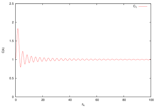
The functional form of this quantity for the scheme considered in this article, (29), has a more complicated form than the corresponding quantities that resulted from the schemes of collapse considered in Perez2006 . Here we reproduce those expressions for comparison with the scheme considered here and with observations. In the first collapse scheme (31), the expectation values for the field and its canonical conjugate momentum after the collapse are randomly distributed within the respective ranges of uncertainties in the pre-collapsed state, and are uncorrelated. The resulting power spectrum has
| (31) |
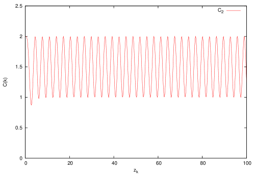
The second scheme considered in Perez2006 only the conjugate momentum changes its expectation value from zero to a value in such range, this second scheme is proposed since in the first-order equation (7) only this variable appears as a source. This leads to a spectrum with
| (32) |
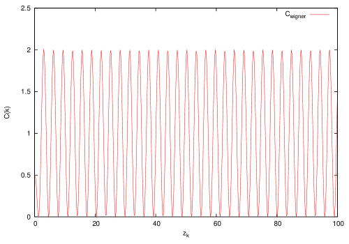
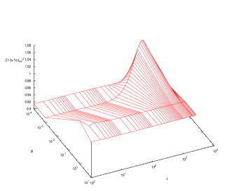
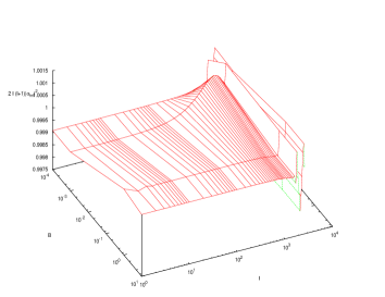
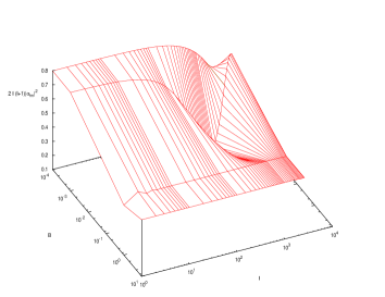
Despite the fact that the expression for looks by far more complicated that , their dependence in is very similar, except for the amplitude of the oscillations (see figures 1(b) and 1(c)). Another interesting fact that can be easily detected in the behaviour of the different schemes of collapse is that if we consider the limit , then and we recover the standard scale invariant spectrum. This does not happen with or (see figure 1).
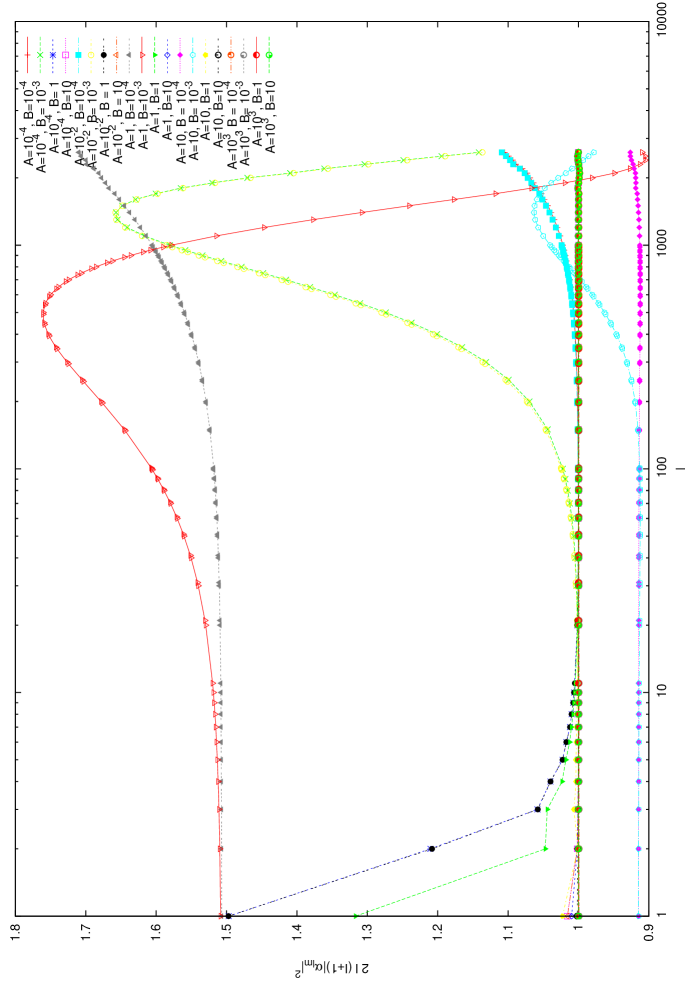
We recall that the standard form of the predicted spectrum is recovered by taking . Therefore, we can consider the issue of how the various collapse schemes approach the standard answer (given the fact that the standard answer seems to fit the observations rather well). In particular we want to investigate how sensitive are the predictions for the various schemes, to small departures from the case where is independent of , which as we argued above would lead to a precise agreement with the standard spectral form. In order to carry out this analysis, we must obtain the integrals (14) for the various collapse schemes characterized by the various functions and . It is convenient to define the adimensional quantity , where and . We will be working under the following assumptions: (1) The changes in scale during the time elapsed from the collapse to the end of inflation are much more significant than those associated the time elapsed from the end of inflation to our days, thus we will use the approximation ; (2) We will explore the sensitivity for small deviations of the “ independent of recipe” by considering a linear departure from the independent characterized by as in order to examine the robustness of the collapse scheme in predicting the standard spectrum. We note that and are adimensional.
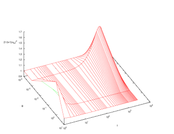
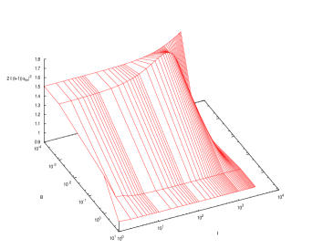
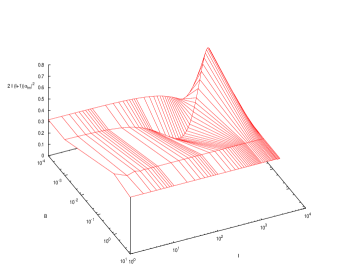
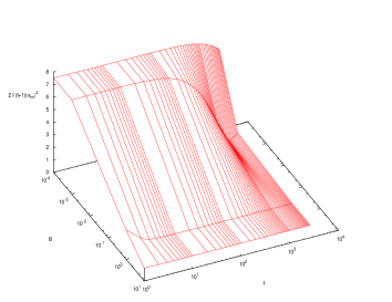
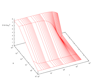
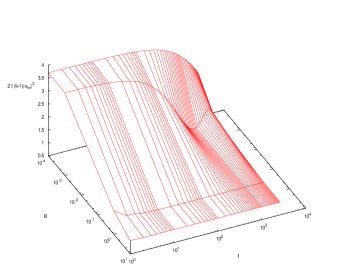
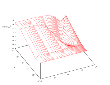
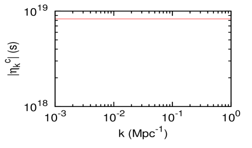
In the figures 2, 3 and 4 reflect the way the spectrum behaves as a function of , were we must recall that standard prediction (ignoring the late physics input of plasma oscillations etc) is a horizontal line. Those graphs represent various values of and chosen to sample a relatively ample domain. The graphs (5, 6 and 7) show the form of the spectrum for various choices for the value of keeping the value of fixed.
It is important at this point remind the reader -in the order to avoid possible misinterpretations- that this graphs are ignoring the effect of late physics phenomena (plasma oscillations, etc.). Our aim, at this stage is to compare this graphs with the scale-invariant spectrum predicted by standard inflationary scenarios (i.e. a constant value for ) and not -directly- with the observed spectrum.
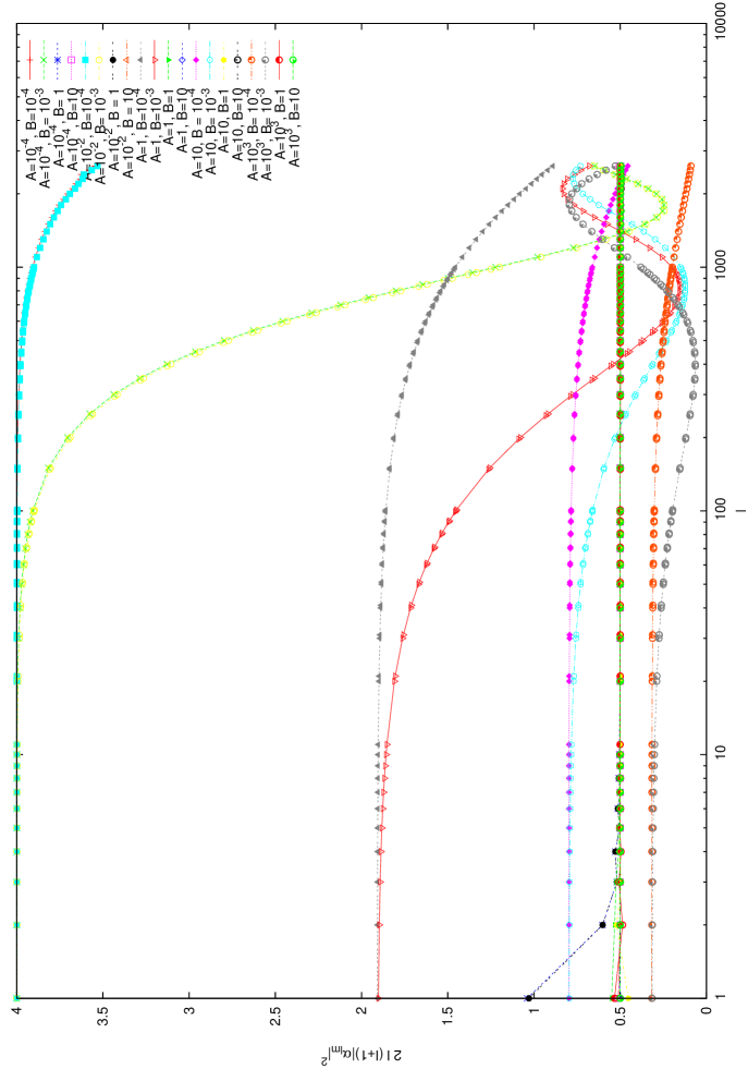
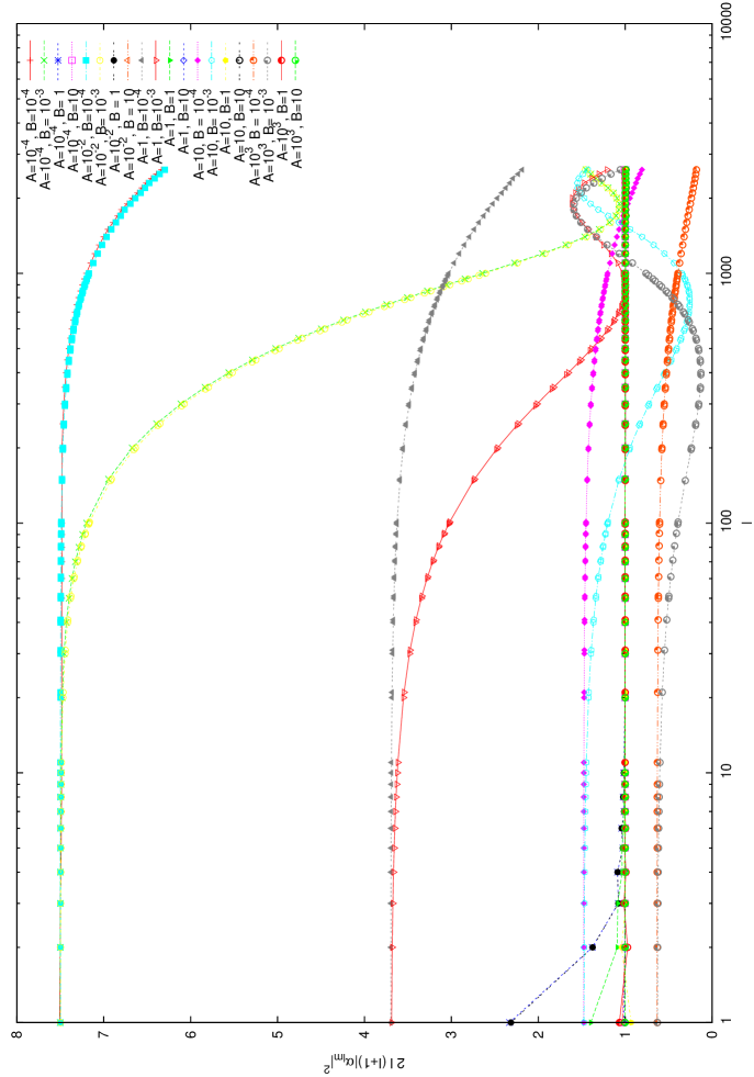
As we observed before the behavior of and is qualitatively similar, the main difference comes from the amplitude of the oscillations of the functional.


From these results we can obtain some reasonable constrains on the values of the and for the different schemes of collapse. We start by defining for a given predicted spectrum the degree of deviation from the flat spectrum to be simply where represents the flat spectrum that would best approximate the corresponding imaginary data and is given by . If we set a bound on the departure from scale invariance up to of 10% measured by (i.e. requiring ) we obtain for the various collapse schemes the corresponding allowed range of values for the parameters and . The results from these analysis are presented in the tables 1, 2 and 3. We see that the restriction of range in becomes weaker for larger values of , something that can be described by stating that the earlier the collapse occurs the larger the possible departures from the behavior .
| 0.0001 | 0.0001 | 6.63019 |
| 0.0001 | 0.001 | 28.3844 |
| 0.0001 | 1 | 0.288273 |
| 0.0001 | 10 | 0.301883 |
| 0.01 | 0.0001 | 6.84475 |
| 0.01 | 0.001 | 28.3706 |
| 0.01 | 1 | 0.282546 |
| 0.01 | 10 | 0.301614 |
| 1 | 0.0001 | 10.1258 |
| 1 | 0.001 | 21.3117 |
| 1 | 1 | 0.247444 |
| 1 | 10 | 0.341509 |
| 10 | 0.0001 | 1.67782 |
| 10 | 0.001 | 15.8869 |
| 10 | 1 | 0.195523 |
| 10 | 10 | 0.384265 |
| 1000 | 0.0001 | 0.44236 |
| 1000 | 0.001 | 1.58567 |
| 1000 | 1 | 0.394892 |
| 1000 | 10 | 0.402706 |
| 0.0001 | 0.0001 | 7.92849 |
| 0.0001 | 0.001 | 53.9872 |
| 0.0001 | 1 | 0.423473 |
| 0.0001 | 10 | 0.249129 |
| 0.01 | 0.0001 | 8.12093 |
| 0.01 | 0.001 | 54.2265 |
| 0.01 | 1 | 0.277929 |
| 0.01 | 10 | 0.251313 |
| 1 | 0.0001 | 21.8266 |
| 1 | 0.001 | 50.6328 |
| 1 | 1 | 0.312876 |
| 1 | 10 | 0.443572 |
| 10 | 0.0001 | 18.4953 |
| 10 | 0.001 | 46.1397 |
| 10 | 1 | 0.917963 |
| 10 | 10 | 0.445398 |
| 1000 | 0.0001 | 28.9085 |
| 1000 | 0.001 | 56.2369 |
| 1000 | 1 | 0.208227 |
| 1000 | 10 | 0.434914 |
| 0.0001 | 0.0001 | 10.0763 |
| 0.0001 | 0.001 | 47.3616 |
| 0.0001 | 1 | 0.506768 |
| 0.0001 | 10 | 0.162458 |
| 0.01 | 0.0001 | 10.2874 |
| 0.01 | 0.001 | 47.494 |
| 0.01 | 1 | 0.359852 |
| 0.01 | 10 | 0.165756 |
| 1 | 0.0001 | 18.445 |
| 1 | 0.001 | 34.1731 |
| 1 | 1 | 0.358535 |
| 1 | 10 | 0.394309 |
| 10 | 0.0001 | 19.3128 |
| 10 | 0.001 | 45.1946 |
| 10 | 1 | 0.51842 |
| 10 | 10 | 0.430548 |
| 1000 | 0.0001 | 28.9273 |
| 1000 | 0.001 | 56.2646 |
| 1000 | 1 | 0.197662 |
| 1000 | 10 | 0.445794 |
We note that we can recover the range of times of collapse for the different values of and . We can solve , therefore . Note that is the comoving radii of the last scattering surface. Considering the radial null geodesics we find , where is the time of the decoupling. The decoupling of photons occurs in the matter domination epoch, so we can use the expression for in terms of the scale factor, using the corresponding solution to the Friedman equation
| (33) |
where we have normalized the scale factor so today is , so, and is the Hubble variable today. The numerical value is Mpc. Henceforth
| (34) |
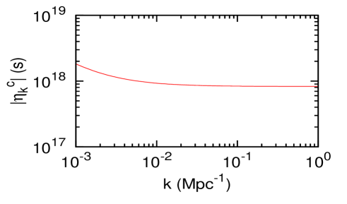
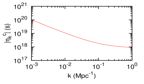
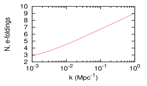
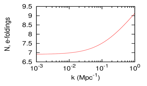
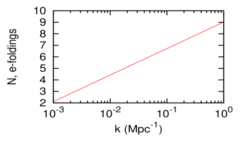
Thus, we can use this formula and calculate the collapse time of the interesting values of we observe in the cosmic microwave background (CMB), namely the range between Mpc-1 Mpc-1. These modes covers the range of the multipoles of interest: , were we made use of the relation999The relation between the angular scale and the multipole is . The comoving angular distance, , from us to an object of physical linear size , is . , if the object is in the LSS, and using the first expression in this footnote, we get . . The collapse times for these modes can be regarded as the times in which inhomogeneities and anisotropies first emerged at the corresponding scales. These collapse times are shown in figure (8) for the best values of given in the tables101010 The reader should keep in mind that our parametrization of the inflationary regime has the conformal time running from large negative values to small negative values (1, 2, 3).
We can compare the value of the scale factor at the collapse time , with the traditional scale factor at “horizon crossing” that marks the “quantum to classical transition” in the standard explanation of inflation: . The “horizon crossing” occurs when the length corresponding to the mode has the same size that the “Hubble Radius”, , (in comoving modes ) therefore, . Thus the ratio of the value of scale factor at horizon crossing for mode and its value at collapse time for the same mode is
| (35) |
Using the best-fit values for the different collapse schemes, we can plot the e-folds elapsed between the modes collapse and its horizon crossing. As we can see in the figure (9) this quantity changes -at most- of one order of magnitude in the range for for the values of and that were considered more reasonable, i.e. , the time of collapse in this range. The door is clearly open for a more in detailed analysis and comparison to the the actual empirical data, whereby one could hope to extract robust information of the type discussed above.
V Discussion
We have considered various, relatively ad hoc recipes for the form of the state of the quantum inflationary field, that results, presumably from a gravitationally induced, collapse of the wave function. The breakdown of unitarity that this entails, is thought to be associated with drastic departures from standard quantum mechanics once the fundamental quantum gravity phenomena come into play. We have not discussed at any length this issue here and have focused in the present treatment as purely phenomenological aspects of the problem.
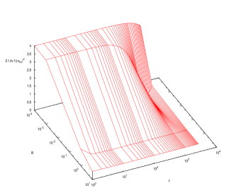
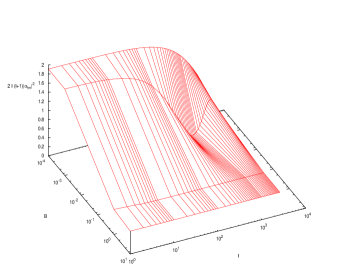
The analysis of the signatures of the different schemes of collapse illustrate various generic points worth mentioning: First, that, depending on the details of the collapse scheme and its parameters, there can be substantial departures in the resulting power spectrum, from the standard scale invariant spectrum usually expected to be a generic prediction from inflation. Of course it is known that there exist other ways to generate modifications in the predicted spectrum, such as considering departures from slow roll and modifications of the inflaton potential and so forth. In the approach we have been following the modifications arise from the details of a quantum collapse mechanism, a feature tied to a dramatic departure from the standard unitary evolution of quantum of physics that we have argued must be invoked if we are to have a satisfactory understanding of the emergence of structure from quantum fluctuations. In fact, by fitting the predicted and observational spectra, these sort of modifications are possible sources of clues about what exactly is the physics behind the quantum mechanical collapse or whatever replaces it. We saw that generically one recovers the standard scale invariant Harrison-Zéldovich spectrum if the collapse time (conformal time) of the modes is such that 111111 This resembles the condition that is sometimes considered in the context of the so called trans-plankian problem. There is however an important difference of what is supposed to occur at the (conformal) time that appears in this condition. In addressing, the trans-plankian problem the time indicates when the mode actually comes into existence. In contrast , in our approach, the mode has existed always -modes are not created or destroyed-, but the state of the field in the corresponding mode changes (or jumps) from the Adiabatic vacuum before the condition to the so called post-collapsed state after this, or a similar condition, is reached.. On the other hand and as shown in detail in Perez2006 the simple generalization of the ideas of Penrose about the conditions that would trigger the quantum gravity induced collapse leads precisely to the such prediction for . We should however keep in mind that, even if something of that sort is operating, the stochastic nature of any sort of quantum mechanical collapse leads us to expect that such pattern would not be followed with arbitrarily high precision. In this regard we have studied the robustness of the various schemes in leading to an almost scale invariant spectrum. To this end we have considered in this work, the simplest (linear) deviations from the behavior of as a function of i.e. we have explored in the three existing collapse schemes the effects of having a time of collapse given by . The results of these studies are summarized in figures 2, 3, 4 and tables 1, 2 and 3, so here we will only point out one of the most salient features: We note that the different collapse schemes lead to different types of departures of the spectrum from the scale invariant one, for instance the schemes and lead naturally to a turning down of the spectrum as we increase .
It is worth noting that a turning down in the spectrum is observed in the CMB data wmap2007 ,which is attributed as a whole, in literature to the Damping Effect121212This effect basically is a damping for the photon density and velocity at scale at the time of decoupling by a factor of , where is the diffusion scale and depends in the physics of the collisions between electrons and photons. Accordingly, the spectrum is also damped as where , for typical cosmological parameters. , i.e. to the fact that inhomogeneities are dampened do the non zero mean-free-path of photons at that time of decoupling Damping . As observed in the figures (3, 4) for some values of we obtain an additional source of “damping” due to fluctuations in the time of collapse about the pattern characterized by . It is expected that the PLANCK probe will provide more information on the spectrum for large values of , so hopefully this characteristic of our analysis could be analyzed and distinguished from the standard damping in order to obtain interesting constraints on the parameters . In fact we believe that one should be able to disentangle the two effects, because in the cases in which our model leads to additional damping in the spectrum, it also predicts that should be a rebound at even higher values of (see figures 2, 3, 4).
However, the most remarkable conclusion, illustrated by the present analysis, is that by focussing on issues that could be thought to be only philosophical and of principle, we have been lead to the possibility of addressing issues pertaining to some novel aspects of physics which could be confronted with empirical observations. Further and more detailed analysis based on direct comparisons with observations are indeed possible, and should be carried out. This together with the foreseeable improvements in the empirical data on the spectrum, particularly in the large region, and the large scale matter distribution studies, should permit even more detailed analysis of the novel aspects of physics that we believe are behind the origin of structure in our universe.
Acknowledgements.
We would like to thank Dr. Jaume Garriaga for suggesting the consideration collapse scheme that follows the Wigner Function. We acknowledge useful discussions on the subject with Dr. Alejandro Perez. This work was supported by the grant DGAPA-UNAM IN119808 in part by a grant from DGEP-UNAM to one of the authors (AUT).References
- [1] Perlmutter, S. et al., Astrophys. J., 483, 565 (1997); Astrophys. J., 517, 565 (1999); Riess, A. G. et al., Astron. J., 116, 1009 (1998); For a recent analysis see W. Michael Wood-Vasey et al.. Astrophys.J. 666 694, (2007). arXiv: astro-ph/0701041
- [2] D.G. York et al., Astron. J. 120 , 1579 (2000); C. Stoughton et al., Astron.J. 123 , 485 (2002); K. Abazajian et al., Astron.J. 126 , 2081(2003).
- [3] D. N. Spergel et al., APJS, 170,377, (2007). arXiv:astro-ph/0603449.
- [4] J.J. Halliwell, Phys. Rev. D, 39, 2912,(1989).
- [5] C. Kiefer Nucl. Phys. Proc. Suppl. 88, 255 (2000) arXiv:astro-ph/0006252; J. Lesgourges, D. Polarski and A. A. Starobinsky, Nucl. Phys. B497, 479 (1997) arXiv:gr-qc/9611019; D. Polarski and A. A. Starobinsky, Classical Quantum Gravity 13 377 (1996) arXiv:gr-qc/9504030; ”Environment Induced Superselection In Cosmology”, W.H. Zurek, Environment Induced Superselection In Cosmology in Moscow 1990, Proceedings, Quantum gravity (QC178:S4:1990), p. 456-472. (see High Energy Physics Index 30 (1992) No. 624); R. Laflamme and A. Matacz Int. J. Mod. Phys. D 2, 171 (1993) arXiv:gr-qc/9303036; M. Castagnino and O. Lombardi, Int. J. Theor. Phys. 42, 1281, (2003), arXiv:quant-ph/0211163; F. C. Lombardo and D. Lopez Nacir, Phys. Rev. D 72, 063506 (2005) arXiv:gr-qc/0506051; J. Martin, Lect. Notes Phys. 669, 199 (2005) arXiv:hep-th/0406011.
- [6] A. Perez, H. Sahlmann, and D. Sudarsky, Class. Quantum Grav., 232317-2354, (2006) arXiv:gr-qc/0508100.
- [7] D. Sudarsky. “The seeds of cosmic structure as a door to new physics”. In Recent Developments in Gravity NEB XII, Napflio,Greece, June 2006. J. Phys. Conf. Ser.68, 012029, (2007) arXiv:gr-qc/0612005.
- [8] D. Sudarsky. “A signature of quantum gravity at the source of the seeds of cosmic structure?” In 3rd International Workshop DICE2006:”Quantum Mechanics between Decoherence and Determinism: New Aspects from Particle Physics to Cosmology”, page 67, Castello di Piombino, Tuscany, Italy, September 2006. J. Phys. Conf. Ser. 67, 012054 (2007) arXiv:gr-qc/0701071.
- [9] C. Kiefer, I. Lohmar, D. Polarski and A. A. Starobinsky in 3rd International Workshop DICE2006: Quantum Mechanics between Decoherence and Determinism: New Aspects from Particle Physics to Cosmology (Castello di Piombino, Tuscany, Italy, 2006), J. Phys. Conf. Ser. 67, 012023 (2007); J.Martin arXiv: 0704.3540; D. Sudarsky in Proceedings of From Quantum to Emergent Gravity: Theory and Phenomenology, Trieste (to be published), arXiv:0712.2795.
- [10] J. B. Hartle. “Quantum Cosmology Problems for the 21st Century”, arXiv: gr-qc/9701022; “The Reduction of the State Vector and Limitations on Measurement in Quantum Mechanics of Closed Systems” in Directions in Relativity. Vol. 2: Proceedings, B.L. Hu and T.A. Jacobson (eds.), Cambridge University Press, Cambridge, 1993. arXiv: gr-qc/9301011.
- [11] R. Penrose. The Emperor’s New Mind. Oxford University Press, 1989; R. Penrose. On gravity’s role in quantum state reduction. In C. Callender and N. Huggett, editors, Physics meets philosophy at the Planck Scale, pages 290–304. Cambridge University Press, 2001; R. Penrose, The Road to Reality: A Complete Guide to the Laws of the Universe (Jonathan Cape, London, 2004).
- Wigner [1932] E. Wigner. Phys. Rev., 40, 749-759, (1932).
- Ballentine [2000] L. E. Ballentine. Quantum Mechanics: A Modern Development. World Scientific Publishing Co. Pte. Ltd., 2000.
- [14] S. Brandt and H. D. Dahmen. The Picture Book of Quantum Mechanics. Springer-Verlag, 2001; E. Wigner. “Quantum mechanical distribution functions revisited”. In W. Yourgrad and A. van der Merwe, editors, Perspectives in Quantum Theory, pages 25–36. Dover, 1971; M. Hillery, R. O’Connell, M. Scully, and E. Wigner, Physics Reports, 106(3), 121-167, (1984).
- [15] W. Hu and M. White. Astrophys.J. 479 (1997) 568 arXiv:astro-ph/9609079; S. Dodelson. Modern Cosmology, chapter 8. Academic Press, 2003.; J.A. Peacock. Cosmological Physics, chapters 15, 18. Cambridge University Press, 2000.; P. Anninos. Computational Cosmology: From the early universe to the Large Scale Structure, Living Rev. Relativity (2001) URL (cited in 2008): http://www.livingreviews.org/lrr-2001-2. A. Jones and A. N. Lasenby, The Cosmic Microwave Background, Living Rev. Relativity 1, (1998), 11. URL (cited on 2008): http://www.livingreviews.org/lrr-1998-11