Boltzmann bias grand canonical Monte Carlo

Abstract

We derive an efficient method for the insertion of structured particles in grand canonical Monte Carlo simulations of adsorption in very confining geometries. We extend this method to path integral simulations and use it to calculate the isotherm of adsorption of hydrogen isotopes in narrow carbon nanotubes (2D confinement) and slit pores (1D confinement) at the temperatures of $20$ K and $77$ K, discussing its efficiency by comparison to the standard path integral grand canonical Monte Carlo algorithm.

We use this algorithm to perform multicomponent simulations in order to calculate the hydrogen isotope selectivity for adsorption in narrow carbon nanotubes and slit pores at finite pressures.

The algorithm described here can be applied to the study of adsorption of real oligomers and polymers in narrow pores and channels.

I Introduction

The grand canonical (GC) Monte Carlo (MC) method is an efficient way to calculate thermodynamic properties of adsorbed fluids via computer simulations. Allen and Tildesley (1989); Landau and Binder (2000) It has recently been extended to take into account quantum diffraction effects using the path integral (PI) formulation of quantum mechanics if the adsorption of light particles, such as helium atoms or hydrogen molecules, is investigated at low temperatures. Wang et al. (1997); Kowalczyk et al. (2007)

Use of the method for the study of hydrogen adsorption in very confining geometries has led to the discovery of a very strong isotope effect. Katorski and White (1964); Moiseyev (1975) The adsorption of hydrogen isotopes in carbon nanotubes has been thoroughly investigated as a function of temperature and nanotube radius, and it has been found that these nanostructured materials might be used, in principle, to obtain a very efficient isotope separation, a phenomenon referred to as “quantum sieving” and studied theoretically for a long time. Beenakker et al. (1995); Wang et al. (1999, 1997); Challa et al. (2001, 2002); Hathorn et al. (2001); Trasca et al. (2003); Lu et al. (2006); Garberoglio et al. (2006); Kowalczyk et al. (2007) Recently the first experimental confirmations have been reported. Hattori et al. (2006); Bondarenko and Alekseev (2007)

From a simulation point of view the PIMC method maps the statistical mechanics of $N$ quantum particles into the statistical mechanics of $N$ ring polymers, each formed by $P$ particles. The mapping is exact in the limit $P\rightarrow\infty$, even though, according to the temperature investigated, convergence of the results can be obtained when $P$ is of the order of 10-100.

The standard path integral grand canonical (PIGCMC) simulation procedure was developed by Johnson and collaborators Wang et al. (1997) who used ring polymer configurations drawn from an ideal gas distribution as insertion candidates. While this method is effective for studying adsorption in large pores, it is very inefficient when applied to very narrow geometries. The reason of this inefficiency stems from the fact that in a strongly confined system at low temperatures the average kinetic energy of the adsorbed particles might be much higher than the average thermal kinetic energy of a free particle. In the path integral formulation this quantity is related to the size of the ring polymers: polymers are smaller - on average - when they represent particles with higher kinetic energy. As a consequence, if one tries to insert ring polymers drawn from a ideal gas distribution at the desired temperature in a strongly confining geometry, the likelihood of a rejection is very high, because the “average” ideal gas configuration just does not fit in the available space within the adsorbent.

This phenomenon has been recognized in the early PIGCMC simulations, since very low acceptance ratios were observed when trying to insert ideal gas ring polymers in very narrow carbon nanotubes. Challa et al. (2002) The same phenomenon has also been observed by independent studies in the case of adsorption in carbon slit pores and and has been called “quantum polymer shrinking” by Kowalczyk et al. Kowalczyk et al. (2007) and it is a consequence of the well known fact that more confining geometries enhance the zero point energy of adsorbed particles. This effect is even more pronounced when the rotational degrees of freedom of the hydrogen molecule are taken into account, leading to a dramatic enhancement of the sieving properties. Garberoglio et al. (2006); Lu et al. (2006); Garberoglio and Johnson (2007)

We propose a new algorithm for insertion moves in classical and quantum (path integral) grand canonical Monte Carlo simulations, which is particularly suitable in the case of strong confinement. We show that the acceptance ratio of insertion moves can be up to two orders of magnitude higher than the one obtained using ideal gas ring polymers as trial configurations. As a consequence the equilibration and production runs of a PIGCMC simulation can be made correspondingly shorter, considerably reducing the time needed for the calculations.

This method, which we call Boltzmann bias grand canonical Monte Carlo, uses as trial configurations ring polymers obtained by an independent path integral Monte Carlo simulation of particles which are adsorbed within the same adsorbent, but do not interact between themselves, so that the “shape” of the ring polymers to be inserted is already the correct one and consequently the insertion candidates are more likely to fit within the confining geometry.

In the following we derive the expressions for the trial and acceptance probability, both in the classical and in the quantum case. Although the Boltzmann bias method is not likely to produce any improvement in classical simulations of structureless particles with respect to other existing algorithms, we present the derivation in detail for the classical case. This will be done to fix the notation before passing on to the quantum case. We also present this algorithm in the case of adsorption of oligomers and polymers within confining geometries.

We will apply the Boltzmann bias method to the calculation of adsorption isotherms and finite pressure selectivities for mixtures of hydrogen isotopes in narrow carbon nanotubes and slit pores, and compare our results with those obtained using the standard PIGCMC method.

The analysis of the efficiency of the Boltzmann bias method will show that one can obtain acceptance ratios up to four orders of magnitude higher than the ones obtained using the standard insertion algorithm, dramatically reducing the amount of time needed to perform the computer simulations.

II Boltzmann bias method

II.1 Classical simulations

The GCMC method is based on the generation of a Markov chain having as equilibrium probability density the quantity

$$P^{(\rm eq)}(x_{1},\ldots,x_{N})=\frac{1}{\Xi}\frac{e^{\beta\mu N}}{N!\Lambda^{3N}}e^{-\beta U(x_{1},\ldots,x_{N})}~{}d^{3}x_{1}\ldots d^{3}x_{N}$$ (1)

where $N$ is the variable number of particles, and $V$, $T$ and $\mu$ are the system’s volume, the temperature and the chemical potential, respectively, which are all kept fixed. The quantity $\Lambda=h/\sqrt{2\pi mk_{B}T}$ is the thermal de Broglie wavelength of the particles of mass $m$ and $\Xi=\sum_{N}e^{\beta\mu N}Q_{N}(V,T)$ is the grand canonical partition function. $Q_{N}(V,T)$ is the canonical partition function,$\beta=1/k_{B}T$ and $k_{B}$ is the Boltzmann constant. Finally, $U(x_{1},\ldots,x_{N})$ is the interaction potential energy between the $N$ particles and/or between the particles and an external potential (which can model, for example, an adsorbent).

The Markov chain is built by moves that either keep the number of particles constant (and for which the standard canonical Monte Carlo algorithms can be used) and moves that change the number of particles in the system. It is usually sufficient to consider moves in which the number of particles is changed by unity.

The expression for the transition probability $W_{i\rightarrow j}$ of the Markov chain between states $i$ and $j$ having $N$ and $N+1$ particles respectively can be obtained by applying, as usual, the detailed balance condition, i.e.

$$\frac{W_{N\rightarrow N+1}}{W_{N+1\rightarrow N}}=\frac{P^{(\rm eq)}_{N+1}}{P^{(\rm eq)}_{N}}=\frac{e^{\beta\mu}}{(N+1)\Lambda^{3}}e^{-\beta\Delta U}~{}d^{3}x_{N+1}$$ (2)

where $\Delta U=U_{N+1}-U_{N}$ is the difference between the potential energy of the two states $i$ and $j$. The transition probability $W$ is written as the product of a trial probability $T$ and an acceptance probability $A$. In the standard grand canonical Monte Carlo algorithm the trial probability for an insertion is such that a test particle is inserted uniformly within the volume and the the probability of a removal is just one, hence

$$\begin{array}[]{rcl}T_{N\rightarrow N+1}&=&\displaystyle\frac{d^{3}x_{N+1}}{V}\\ T_{N+1\rightarrow N}&=&1\end{array}$$ (3)

so that the ratio between the acceptance probabilities corresponding to the insertion into and removal from the system of a particle is

$$\frac{A_{N\rightarrow N+1}}{A_{N+1\rightarrow N}}=\frac{V}{(N+1)\Lambda^{3}}e^{\beta\mu}e^{-\Delta U},$$ (4)

a condition that can be satisfied, e.g., by the standard Metropolis choice

$$\begin{array}[]{rcl}A_{N\rightarrow N+1}&=&\min\left[1,\displaystyle\frac{V}{(N+1)\Lambda^{3}}~{}e^{\beta\mu}e^{-\Delta U}\right]\\ A_{N+1\rightarrow N}&=&\min\left[1,\displaystyle\frac{(N+1)\Lambda^{3}}{V}~{}e^{-\beta\mu}e^{\Delta U}\right]\end{array}$$ (5)

The Boltzmann bias methods stems now from the fact that in many cases the interaction potential energy can be written as the sum of the potential energy of interaction with the fluid particles between themselves ($U_{\rm FF}$) and the interaction potential energy with a substrate ($U_{\rm SF}$), the latter being additive in the number of particles, i.e.

$$U({x_{1},\ldots,x_{N}})=U_{\rm FF}(x_{1},\ldots,x_{N})+U_{\rm SF}(x_{1},\ldots,x_{N})=U_{\rm FF}(x_{1},\ldots,x_{N})+\sum_{k=1}^{N}u_{\rm SF}(x_{k})$$ (6)

so that one can devise an insertion move such that the probability of insertion within the volume $V$ is not uniform, but proportional to the Boltzmann factor of the solid-fluid interaction potential of the particle to be inserted, $\exp\left[-\beta u_{\rm SF}(x_{N+1})\right]$. One can then write the trial probability for an insertion as

$$T_{N\rightarrow N+1}=\frac{\exp\left[{-\beta u_{\rm SF}(x_{N+1})}\right]~{}d^{3}x_{N+1}}{\displaystyle\int\exp\left[{-\beta u_{\rm SF}(x_{N+1})}\right]~{}d^{3}x_{N+1}}\equiv\frac{\exp\left[{-\beta u_{\rm SF}(x_{N+1})}\right]~{}d^{3}x_{N+1}}{V~{}e^{-\beta\bar{\mu}}}$$ (7)

where the last equality defines the quantity $\bar{\mu}$. With this choice for the trial probability of an insertion (leaving $T_{N+1\rightarrow N}=1$), one gets for the acceptance probability the ratio

$$\frac{A_{N\rightarrow N+1}}{A_{N+1\rightarrow N}}=\frac{V}{(N+1)\Lambda^{3}}e^{\beta(\mu-\bar{\mu})}e^{-\Delta U_{\rm FF}(x_{1},\ldots,x_{N+1})}$$ (8)

that depends only on the difference of the fluid-fluid potential energy between the original configuration and the trial one.

One way to insert particles with the trial probability given by Eq. (7) is to perform, in parallel with the grand canonical simulation, a standard canonical Monte Carlo simulation of some particles within a similar box and at the same temperature. In this second simulation the particles interact only with the substrate and not among themselves, so that at equilibrium they sample the distribution given by Eq. (7). One can then get the coordinates for the GCMC trial insertions by drawing particles’ positions from the configurations generated by this second simulation.

In the case of classical adsorption of structureless particles this method is not particularly more efficient than other standard methods based on the insertion in the subvolume of the simulation cell where the solid-fluid potential energy is less than a given threshold. This free volume $V_{\rm free}$ can be easily pre-calculated and used in the standard grand canonical algorithm for insertions, Eq. (3), instead of the whole cell volume $V$.

In the case of classical adsorption of molecules, the detailed balance condition (2) can be written as

$$\frac{W_{N\rightarrow N+1}}{W_{N+1\rightarrow N}}=\frac{e^{\beta\mu}}{(N+1)\Lambda^{3}}e^{-\beta\Delta U_{\rm FF}}e^{-\beta U_{\rm SF}(x^{\rm CM}_{N+1},\xi)}e^{-\beta U_{\rm int}(\xi)}~{}d^{3}x^{\rm CM}_{N+1}d\xi$$ (9)

where $x^{\rm CM}_{N+1}$ denotes the center of mass position and $\xi$ are the variables describing the intra-molecular degrees of freedom (such as Euler angles in the case of small rigid molecules or torsion angles for small oligomers). The quantity $U_{\rm int}(\xi)$ is just the internal energy corresponding to the configuration given by the coordinates $\xi$. One can see from Eq. (9) that the transition probability depends on the internal state of the molecule $\xi$ as well as the position of the center of mass for the trial insertion. In the limit of low density the fluid-fluid contribution to the acceptance probability can be neglected and this quantity is mainly determined by the solid-fluid part of the interaction. In the case of adsorption in narrow geometries, many of the trial configurations $\xi$ for a given value of the center of mass position $x^{\rm CM}_{N+1}$ are likely to be rejected, since they would result in strong overlaps of parts of the molecule with the adsorbent. In this case a much greater acceptance ratio could be obtained if the configurations $\xi$ were chosen among the ones most likely to fit at a given position $x^{\rm CM}_{N+1}$. The Boltzmann bias method proposed here is based on choosing the the trial configurations with a probability proportional to the Boltzmann factor of the molecule to be inserted at the position $x^{\rm CM}_{N+1}$, i.e.

$$T_{N\rightarrow N+1}\propto e^{-\beta U_{\rm SF}(x^{\rm CM}_{N+1},\xi)}e^{-\beta U_{\rm int}(\xi)}~{}d^{3}x^{\rm CM}_{N+1}d\xi.$$ (10)

By writing the normalization factor as

$$Ve^{\beta\bar{\mu}}=\int e^{-\beta U_{\rm SF}(x^{\rm CM}_{N+1},\xi)}e^{-\beta U_{\rm int}(\xi)}~{}d^{3}x^{\rm CM}_{N+1}d\xi$$ (11)

one obtains for the acceptance probability an expression analogous to the one reported in Eq. (8). The trial configurations can be easily generated by running an $NVT$ simulation of molecules within the adsorbent, with the fluid-fluid interaction switched off.

Since the solid-fluid interaction has already been taken into consideration by the choice of the trial probability, the acceptance probability now depends on the values of the fluid-fluid interaction between the molecule to be inserted and the ones already present within the simulation box, as well as on the value of the renormalized chemical potential $\mu-\bar{\mu}$. One can then expect a very high acceptance ratio for all the thermodynamic state points where the density of the adsorbed molecules is not liquid-like.

II.2 Path integral simulations

The path integral grand canonical method is based on the Trotter factorization of the many-body Hamiltonian. The quantum partition function of $N$ interacting particles can be written as

$$Q_{N}(V,T)=\frac{1}{N!}\sum_{\pi}\langle\exp\left[-\beta(\hat{T}+\hat{V})\right]P_{\pi}\rangle$$ (12)

where $\hat{T}$ and $\hat{V}$ are the kinetic and potential energy operators, respectively, and the expectation value is taken over a complete set of $N$ particle states. The sum is over all the permutations $\pi$ of the particles, represented in the Hilbert space by the operator $P_{\pi}$ which also takes into account the bosonic or fermionic nature of the particles. In the following we will not consider effects due to quantum statistics and hence we will approximate the sum with its leading term, corresponding to the identity permutation. This is a good approximation as long as the thermal de Broglie wavelength $\Lambda$ does not exceed the hard core radius of the particles under consideration. Feynman (1998) By using the Trotter formula

$$e^{\hat{A}+\hat{B}}=\lim_{P\rightarrow\infty}\left(e^{\hat{A}/P}e^{\hat{B}/P}\right)^{P}$$ (13)

with a finite but large enough Trotter index $P$, the quantum partition function of $N$ particles can be mapped into the classical partition function of $NP$ particles, such that each original particle corresponds to a ring polymer of $P$ “beads”. Ceperley (1995) The beads within each polymer interact with their two nearest neighbors via an harmonic interaction, and we will call this part of the interaction “internal”. Denoting by $X_{i}=\{x^{(1)}_{i},\ldots,x^{(P)}_{i}\}$ the $3P$ coordinates of the beads of the ring polymer corresponding to the $i$-th particle, and applying the same reasoning as described before in the classical case, one obtains for the path integral case

$$\frac{W_{N\rightarrow N+1}}{W_{N+1\rightarrow N}}=\frac{1}{N+1}\left(\frac{P^{3P/2}}{\Lambda^{3P}}\right)e^{\beta\mu}e^{-\beta\Delta\overline{U_{\rm FF}}(X_{1},\ldots,X_{N+1})}e^{-\beta\overline{U_{\rm SF}}(X_{N+1})}e^{-\beta U_{\rm int}(X_{N+1})}~{}d^{3}X_{N+1}$$ (14)

where we have defined

$$\overline{U_{\rm FF}}(X_{1},\ldots,X_{N}) = \frac{1}{P}\sum_{p=1}^{P}\sum_{i<j=1}^{N}u_{\rm FF}(|x^{(p)}_{j}-x^{(p)}_{i}|)$$ (15)

$$\overline{U_{\rm SF}}(X_{N+1}) = \frac{1}{P}\sum_{p=1}^{P}u_{\rm SF}(x^{(p)}_{N+1})$$ (16)

$$U_{\rm int}(X_{N+1}) = k_{B}T~{}\frac{K}{2}\sum_{p=1}^{P}\left|x^{(p)}_{N+1}-x^{(p+1)}_{N+1}\right|^{2},$$ (17)

$K=2\pi P/\Lambda^{2}$, $\Delta\overline{U_{FF}}(X_{1},\ldots,X_{N+1})=\overline{U_{\rm FF}}(X_{1},\ldots,X_{N+1})-\overline{U_{\rm FF}}(X_{1},\ldots,X_{N})$ and we have used the convention $x^{(P+1)}_{N+1}=x^{(1)}_{N+1}$. In the path integral GCMC case the ratio between the transition probabilities connecting states with different number of particles depends also on the internal state of the added polymer and it is customary to draw internal states from an ideal gas path integral simulation. Wang et al. (1997)

This way of proceeding is highly inefficient in the case of strong confinement, where one expects that the distribution of shapes for the adsorbed ring polymers, having to account for a high kinetic energy due to Heisenberg indetermination, will be considerably different from the equilibrium distribution of an ideal gas. In particular it turns out that polymers corresponding to states of higher kinetic energy tend to have a smaller size. Kowalczyk et al. (2007) As a consequence the probability of rejecting an insertion move is particularly high, because almost all of the ideal gas ring polymer configurations do not easily fit into the available space within the adsorbent.

In this case the Boltzmann bias method is likely to improve the situation. Instead of drawing a ring polymer configuration from an ideal gas distribution, the trial insertion probability is chosen to be proportional to the probability of finding an isolated ring polymer within the adsorbent, i.e.

$$T_{N\rightarrow N+1}\propto\left(\frac{P^{3P/2}}{\Lambda^{3P}}\right)e^{-\beta\overline{U_{\rm SF}}(X_{N+1})}e^{-\beta U_{\rm int}(X_{N+1})}~{}d^{3}X_{N+1}$$ (18)

By using the change of variables

$$\begin{array}[]{ccc}r&=&x^{(1)}_{N+1}\\ \Delta r_{1}&=&x^{(2)}_{N+1}-x^{(1)}_{N+1}\\ &\cdots&\\ \Delta r_{P-1}&=&x^{(P)}_{N+1}-x^{(P-1)}_{N+1}\end{array}$$ (19)

the normalization factor can be written as the integral

$$\frac{1}{\Lambda^{3}}\int e^{-\beta\overline{U_{\rm SF}}(r,\Delta r_{1},\ldots,\Delta r_{P-1})}F_{\rm ring}(\Delta r_{1},\ldots,\Delta r_{P-1})~{}\prod_{p=1}^{P-1}\Delta r_{p}~{}d^{3}r=Ve^{-\beta\bar{\mu}}$$ (20)

where $F_{\rm ring}(\Delta r_{1},\ldots,\Delta r_{P-1})$ is the probability of having a configuration of an ideal gas ring polymer with separations $\Delta r_{p}$ between the neighboring beads, and it is derived in Appendix A. The last equality defines the quantity $\bar{\mu}$ analogously to the classical definition given in Eq. (7).

With these definitions the ratio of the acceptance probabilities for moves which change the number of particles in the path integral case is

$$\frac{A_{N\rightarrow N+1}}{A_{N+1\rightarrow N}}=\frac{V}{(N+1)\Lambda^{3}}e^{\beta(\mu-\bar{\mu})}e^{-\Delta\overline{U_{\rm FF}}(X_{1},\ldots,X_{N+1})}$$ (21)

completely analogous to the classical case of Eq. (8). By “undoing” the Trotter factorization in Eq. (20) one can show that

$$Ve^{-\beta\bar{\mu}}=\Lambda^{3}\left\langle\exp\left[-\beta\left(\frac{\hat{p}^{2}}{2m}+u_{\rm SF}(\hat{x})\right)\right]\right\rangle=\Lambda^{3}\sum_{i}e^{-\beta E_{i}}$$ (22)

where $E_{i}$ are the quantum energy levels of a single particle interacting with the adsorbent.

The Boltzmann bias PIGCMC method is particularly efficient in the case where adsorption is simulated in materials having an (approximate) continuous translational symmetry as it happens, e.g., in carbonaceous materials such as carbon nanotubes and slit pores, where it has been shown that the corrugation of the potential energy can be neglected without sacrificing accuracy. Challa et al. (2001) In this case the ring polymer configurations for trial insertions can be further translated by a random value along the direction(s) of translational symmetry. This prescription avoids the need to wait for the polymers in the zero-pressure simulation box to diffuse away from positions already used for trial insertions.

In the case of simulations in geometries that do not possess continuous translational symmetry, as it might happen if the effect of nanotube corrugation on adsorption had to be addressed or in the case of adsorption in amorphous materials, one should perform long stages of $NVT$ MC in the zero-pressure box until a new configuration, uncorrelated with the previous one, is generated. This is necessary in order for the new polymers used for trial insertions not to end up on top of polymers already present in the simulation box, resulting in a certain rejection.

In the general case another method for generating trial polymers, which seems particularly suited for path integral simulations, could be used. One starts from configurations where $N$ independent classical point particles are adsorbed at the target temperature $T$ (which can be generated very efficiently, even in a parallel environment, either by GCMC or molecular dynamics), and use them to build $N$ ring polymers where all the beads are at the position of the corresponding classical particles. These polymers can be efficiently equilibrated using hybrid MC Duane et al. (1987); Wang et al. (1997) and then used as insertion candidates. This approach might be more efficient than the direct one outlined above, and its performance will be analyzed in future studies.

There is another issue to be addressed in the case of simulation of adsorption in more general geometries, i.e. the calculation of the parameter $\bar{\mu}$. In a general geometry the calculation of the energy levels of a single particle, needed to compute $\bar{\mu}$ according to Eq. (22), can be very computationally demanding and in this case it could be worth it using directly Eq. (20). In fact the left hand side of Eq. (20) consists of a three dimensional integration over the variable $r$ of the $e^{-\beta\overline{U_{\rm SF}}(r,\Delta r_{1},\ldots,\Delta r_{P-1})}$ averaged over ring polymer configurations drawn from an ideal gas distribution, which can be generated rather efficiently. Fosdick and Jordan (1966)

III Adsorption in narrow carbon nanotubes

III.1 Pure fluid isotherms

In order to validate the Boltzmann bias method we compare the results with standard path integral grand canonical Monte Carlo simulations of adsorption in carbon nanotubes, where insertion moves are performed by taking ring polymer configurations from an ideal gas simulation performed in parallel with the main computation.

We model the carbon nanotubes as smooth tubes of given geometrical radius $R$. The solid-fluid interaction depends only on the distance of the particle from the tube axis, and we used the expression for the average potential reported in Refs. LaBrosse, ; Stan and Cole, 1998; Zhang et al., 2004. We chose two values of the geometrical radius: $R=3.6$ Å that corresponds to the (2,8) tube and $R=3.1$ Å that corresponds to the (3,6) tube.

Earlier path integral simulations of hydrogen adsorption in these tubes showed that at the temperature of $T=20$ K, quantum effects are very important to describe the actual behavior of hydrogen adsorbed in the (3,6), and moderately important in the case of the (2,8) tube. Challa et al. (2001, 2002) At a higher temperature of $T=77$ K, quantum effects on adsorption in the (2,8) tube are expected to be smaller.

In our simulations the fluid-fluid interaction between hydrogen atoms is assumed to be of the Lennard-Jones type, with the Buch parameters Buch (1994) $\varepsilon_{\rm HH}/k_{B}=34.2$ K and $\sigma_{\rm HH}=2.96$ Å, and the solid-fluid hydrogen-carbon interaction is calculated using the Lorentz-Berthelot mixing rules Allen and Tildesley (1989) together with the Steele parameters Steele (1978) for the carbon atom, $\varepsilon_{\rm CC}/k_{B}=28.0$ K and $\sigma_{\rm CC}=3.4$ Å. The quantity $\bar{\mu}$ appearing in Eq. (21) has been calculated using Eq. (22). The energy levels of a single hydrogen particle interacting with a carbon nanotube have been obtained by direct diagonalization of the quantum Hamiltonian, using as a basis set the eigenfunctions of a free particle confined within a rigid cylinder of radius $R$. In the case of the (3,6) nanotube, the first 183 energy states of the free particle were sufficient to reach convergence, whereas in the case of the (2,8) tube we obtained convergence of the results using 226 states. The values of $\bar{\mu}$ as well as other relevant single particle properties of hydrogen isotopes confined in carbon nanotubes are reported in Table 1. The results of these single particle calculations were used to fix the value of the Trotter number $P$ as a function of the temperature: we performed path integral canonical simulations of hydrogen adsorbed within the tubes switching off the interparticle interaction, progressively increasing the value of $P$ until we obtained the same average values for the kinetic and potential energies as those reported in Table 1. We reached convergence using $P=64$ for H₂ at $T=20$ K and using $P=16$ for H₂ at $T=77$ K. The same values of the Trotter index $P$ obtained for H₂ were used for the other isotopes.

Nanotube type	Adsorbate	Temperature (K)	$\bar{\mu}/k_{B}$ (K)	Kinetic Energy/$k_{B}$ (K)	Potential Energy/$k_{B}$ (K)
(2,8)	H2	20	$-1245$	124.0	$-1392$
(2,8)	T2	20	$-1314$	69.1	$-1428$
(2,8)	H2	77	$-1054$	167.4	$-1383$
(2,8)	T2	77	$-1088$	132.5	$-1404$
(3,6)	H2	20	$-281.3$	329.9	$-629.7$
(3,6)	T2	20	$-524.3$	187.2	$-751.0$
(3,6)	H2	77	$-99.05$	358.6	$-628.6$
(3,6)	T2	77	$-281.0$	219.5	$-747.7$

Table 1: Single particle properties of hydrogen isotopes confined in carbon nanotubes, obtained by direct diagonalization of the single particle Hamiltonian. The quantity $\bar{\mu}$ is defined in Eq. (22).

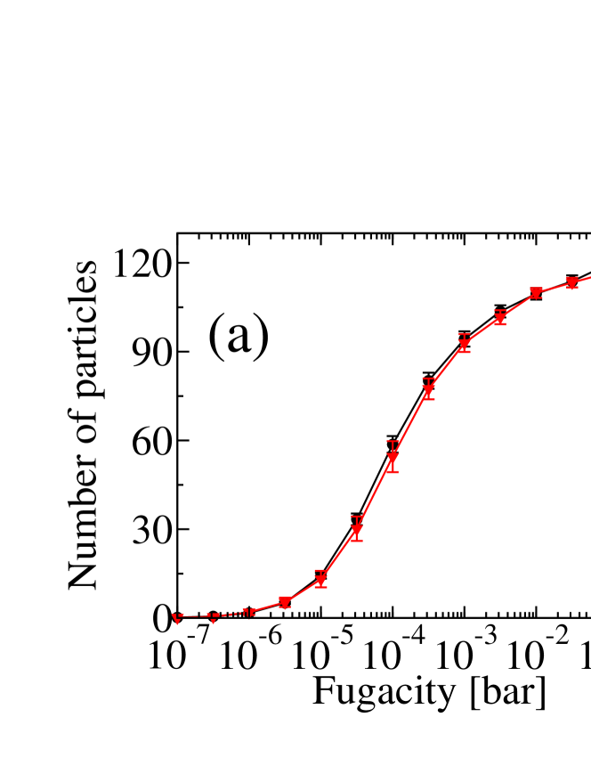
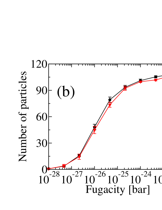
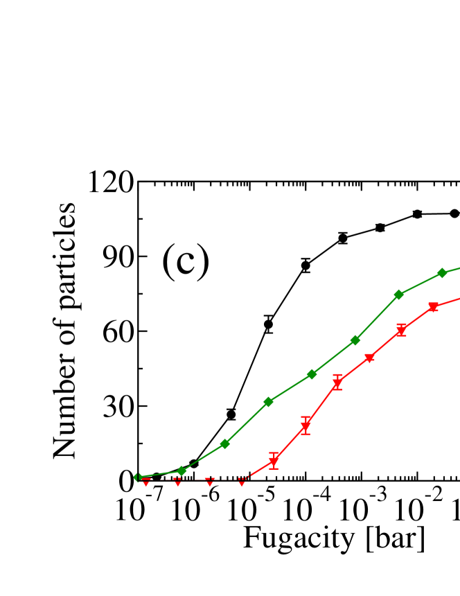
We show in Fig. 1 the adsorption isotherms obtained using both the Boltzmann bias method and the standard procedure for path integral grand canonical Monte Carlo. Wang et al. (1997)

Figure 1: Isotherms of adsorption for hydrogen in carbon nanotubes. (a) (2,8) tube at $T=77$ K, (b) (2,8) tube at $T=20$ K and (c) (3,6) tube at $T=20$ K. The circles denote the results using the Boltzmann bias method, whereas the triangles are the results of simulations using ideal gas ring polymers as insertion candidates. The diamonds in panel (c) are the result of a standard PIGCMC calculation with twice as many MC steps as the other one.

All of the simulations have been performed using $1.5\times 10^{6}$ MC moves per thermodynamic point, after $7.5\times 10^{5}$ moves for equilibration. We consider adsorption in an isolated nanotube of height $Z=400$ Å. Out of 100 Monte Carlo moves, 80 were insertion/deletion attempts and 20 were hybrid MC moves. Duane et al. (1987); Wang et al. (1997)

A first test on the efficiency of the Boltzmann bias method is performed by calculating the adsorption of hydrogen in the (2,8) tube at $T=77$ K. The results of the Boltzmann bias method are compared with the standard prescription for insertion moves in Fig. 1(a), where it is shown that the two methods lead to the same results as far as adsorption is concerned.

The results for the same tube at the lowest temperature, shown in Fig. 1(b) show a slight disagreement, especially in the region around saturation. The isotherms obtained with the two methods for the (3,6) tube at $T=20$ K, reported in Fig. 1(c), are significantly different. The origin of the difference is due to the poor performance of the standard insertion method, that results in a very high rejection rate and hence in a poor convergence towards the equilibrium density. The result of the standard PIGCMC simulation of H₂ adsorption in the (3,6) tube using twice as many steps for equilibration and production, also reported in Fig. 1(c), confirms this observation. As is apparent this second isotherm tends to converge to the correct result, but still shows evident signs of poor equilibration.

Figure 2: Insertion and deletion acceptance ratios for the production runs of the grand canonical simulations. (a) (2,8) tube at $T=77$ K, (b) (2,8) tube at $T=20$ K and (c) (3,6) tube at $T=20$ K. The circles denote the acceptance ratios obtained using the Boltzmann bias method, whereas the triangles are the acceptance ratios from simulations using ideal gas ring polymers as insertion candidates. The solid lines join the points corresponding to the deletion acceptance ratios (not highlighted by any symbol).

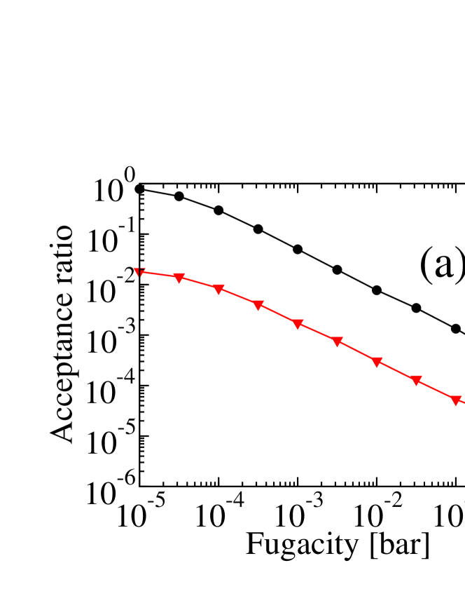
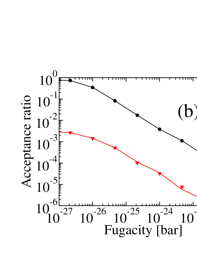
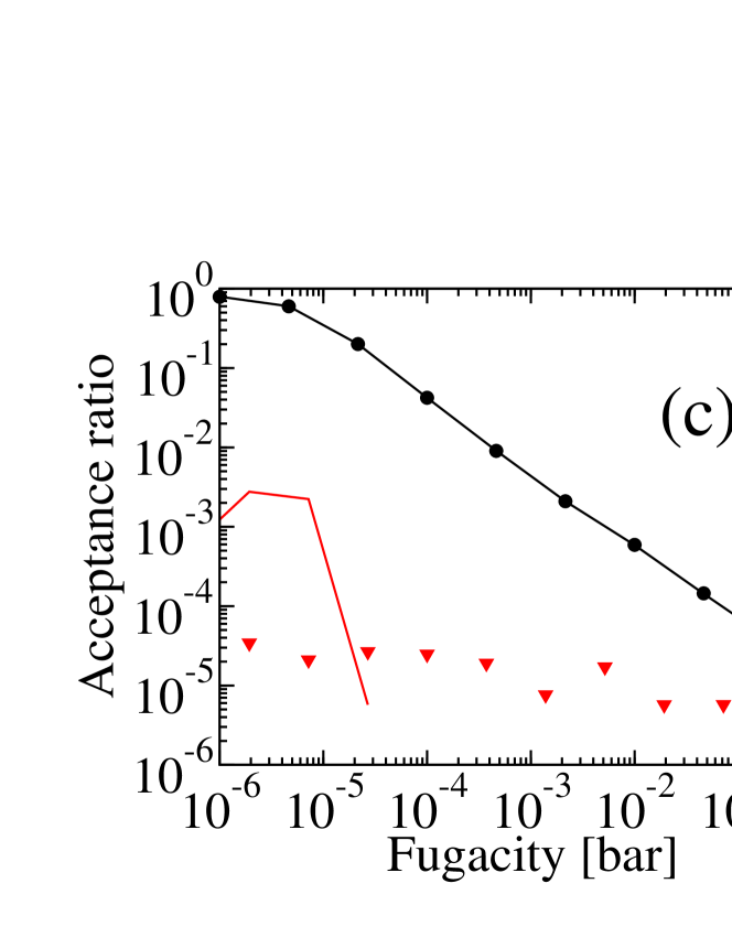
In order to prove this fact, we show in Fig. 2 the insertion and deletion acceptance ratios for all the simulations we have performed.

We notice that the insertion and deletion acceptance ratios have the same values for each state point, except than in the case of the (3,6) tube simulated using the standard practice of inserting ideal gas ring polymers. A simulation run that achieves the same acceptance ratios for insertion and deletion is well equilibrated. The fact that this situation is not verified in the (3,6) tube using standard moves means that equilibration has not been achieved even after $7.5\times 10^{5}$ steps.

Under the same conditions the Boltzmann bias method does not show any sign that convergence has not been reached, and we have checked that one obtains the same isotherm using a larger number of Monte Carlo moves ($2.5\times 10^{6}$ for production and half as many for equilibration, result not shown).

We notice that at each thermodynamic point that has been investigated the acceptance ratios for the Boltzmann bias method are at least one to two order of magnitude higher than the ones obtained using the standard method, and they can be over four orders of magnitude higher than the standard method in very confining geometries at low pressure, such as it happens in the case of hydrogen adsorption at $T=20$ K in (3,6) tube (see Fig. 2(c)).

As might have been expected, the acceptance ratio decreases as the density of adsorbed molecules is increased. This is due to the higher probability of overlap between the particle to be inserted and the particles already present in the simulation cell as the density of adsorbed molecules is increased. In order to raise the acceptance ratio in this case, other kinds of biases can be considered, such as the configuration-bias Monte Carlo. In any case the acceptance ratios for the Boltzmann bias method are one to two orders of magnitude higher than the acceptance ratios obtained using ideal gas ring polymers as candidates. This means that simulations using the Boltzmann bias method need one to two order of magnitude less steps to achieve equilibration as the standard method.

III.2 Zero and finite pressure selectivity in narrow tubes

Nanotube type	Mixture	Temperature (K)	Zero pressure selectivity
(3,6)	T2/H2	20	181000
(3,6)	T2/H2	77	10.5
(3,6)	D2/H2	20	5000
(3,6)	D2/H2	77	5.5
(2,8)	T2/H2	20	32
(2,8)	T2/H2	77	1.55
(2,8)	D2/H2	20	12.5
(2,8)	D2/H2	77	1.40

Table 2: Zero pressure selectivities of hydrogen mixtures in carbon nanotubes

As is well known quantum diffraction effects result in different adsorption properties of various isotopes of the same specie, a phenomenon which is particularly evident at low temperatures and under conditions of strong confinement. Katorski and White (1964); Moiseyev (1975); Beenakker et al. (1995); Wang et al. (1999); Challa et al. (2001, 2002); Garberoglio et al. (2006); Lu et al. (2006); Garberoglio and Johnson (2007)

The differential adsorption of two species $A$ and $B$ is measured by the selectivity $S(A/B)$, defined as

$$S(A/B)=\frac{x_{A}/x_{B}}{y_{A}/y_{B}}$$ (23)

where $x_{i}$ is the molar fraction of specie $i$ in the adsorbed phase, and $y_{i}$ is the molar fraction of the same specie in the gas phase, under conditions of thermodynamic equilibrium. When the pressure is so low that the fluid-fluid interaction between the particles can be neglected, the selectivity can be written as a function of the single particle energy levels of species $A$ and $B$ in the adsorbed phase Challa et al. (2002)

$$S_{0}(A/B)=\left(\frac{m_{B}}{m_{A}}\right)^{3/2}\frac{Q_{A}}{Q_{B}}$$ (24)

where $m_{i}$ are the masses of the two species and $Q_{i}$ is the single particle partition function

$$Q_{i}=\sum_{k}\exp\left(-\beta E^{(i)}_{k}\right)$$ (25)

It can be seen that, in the limit $T\rightarrow 0$, the selectivity is a function of the difference of the zero point energies of the two adsorbed species. Values of the zero pressure selectivity for mixtures of hydrogen isotopes adsorbed in carbon nanotubes are reported in Tab. 2. As might be expected, the selectivity is higher when the mass ratio between the isotopes is higher (all other things being equal), and has a strong temperature dependence. The values reported there can be compared with the values reported in literature for molecular sieves (like zeolites) used in gas separation, where typical values are in the range 10-100, depending on the components of the mixture to be separated. Sridhar et al. (2007); Saufi and Ismail (2004)

Challa et al. have investigated the effect of finite pressure on the selectivity, by performing multicomponent grand canonical path integral Monte Carlo simulations and calculating the selectivity directly from the definition of Eq. (23). They noted a progressive inefficiency in the acceptance ratios for insertion especially at high pressures, and hence were unable to investigate the finite pressure selectivity in conditions of strong confinement.

Figure 3: Selectivity for a T₂/H₂ mixture in the (3,6) carbon nanotube at $T=20$ K as a function of pressure. The simulation has been performed by assuming a mole fraction of T₂ in the bulk phase equal to $y_{\rm{T}_{2}}=5\times 10^{-6}$. The horizontal dashed line corresponds to the zero pressure value, reported in Tab. 2.

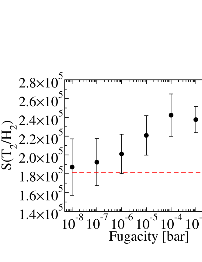
The use of the Boltzmann biased algorithm allows one to gain a factor of 100 in the insertion efficiency, and correspondingly reduce the time needed for equilibration. The results of our simulations for the pressure dependence of the T₂/H₂ selectivity in the (3,6) nanotube are reported in Fig. 3. We have used nanotubes of different length for different pressures: the nanotube lengths were adjusted to have between 150 and 300 particles in the system after equilibration. In order to have an almost equal amount of hydrogen and tritium within the simulation cell we have chosen to perform the simulation by imposing a bulk mole fraction of T₂ equal to $y_{\rm{T}_{2}}=5\times 10^{-6}$. We have used $2\times 10^{5}$ steps for equilibration and $4\times 10^{5}$ steps for production at each state point. The probability of performing an insertion/deletion has been set to 0.8.

One can see that, according to what has been observed in analogous confining geometries, the selectivity actually increases from its zero pressure value and tends to saturate to a value which is some 40% higher that the zero pressure one. This behavior can be understood using a simple mean field model by assuming that, upon saturation, the particles are uniformly arranged within the tube, so that each particle is confined also in the direction of the tube axis. Using the simple theory of Eq. (24), the selectivity upon saturation can be approximately written as the zero pressure selectivity times the selectivity of a one dimensional harmonic oscillator corresponding to the motion along the tube axis. A simple calculation shows that one does indeed get the right magnitude of the increase. Garberoglio and Johnson (2007)

IV Adsorption and selectivity in slit pores

We have also applied our algorithm to the calculation of adsorption isotherms and quantum sieving effects of hydrogen in a narrow slit pore. We have modeled a slit pore as being formed by two graphite planes separated by a distance $H$ along the direction $z$, using the same parameters for carbon–hydrogen interaction as in the case of nanotubes described above. We have obtained a smooth solid-fluid interaction potential $v_{\rm slit}(z)$ by averaging the values of the potential obtained by atomistic calculation over planes at constant height $z$. As a result of this approximation the quantum states of a particle adsorbed within the slit pore are the product of free particle states corresponding to the motion along the $xy$ plane and states coming from the confined motion along the $z$ axis, which have been calculated by numerical diagonalization of the 1D Hamiltonian in the free particle basis. We have reached convergence by using the first 1024 plane waves. We have chosen to investigate in detail only the pore width of $H=5.7$ Å, because this is the narrowest slit still presenting a bound state for adsorbed hydrogen, according to our model.

Adsorbate	Temperature (K)	$\bar{\mu}/k_{B}$ (K)	Kinetic Energy/$k_{B}$ (K)	Potential Energy/$k_{B}$ (K)
H2	20	$-173.2$	205.4	$-361.8$
D2	20	$-273.5$	147.7	$-411.3$
T2	20	$-316.1$	123.0	$-433.2$
H2	77	$-112.6$	262.4	$-361.7$
D2	77	$-193.2$	205.1	$-410.9$
T2	77	$-222.4$	181.1	$-432.2$

Table 3: Single particle properties of hydrogen isotopes confined in a slit pore with $H=5.7$ Å, obtained by direct diagonalization of the single particle Hamiltonian. The quantity $\bar{\mu}$ is defined in Eq. (22).

We report in Tab. 3 the average kinetic and potential energies of single hydrogen isotopes confined within the $H=5.7$ Å slit pore. We notice that the average potential energies do not change very much with increasing temperature, a signature of the fact the the first excited state is very well separated from the ground state for all the three isotopes. The smallest separation is observed for T₂ and is of the order of $\Delta E/k_{B}=412$ K. As a consequence the hydrogen isotopes have a very low probability of being in the first excited state at the temperatures used in this study, and the temperature dependence of the kinetic energies reported in Tab. 3 comes from the different average kinetic energies corresponding to the motion along the $xy$ plane.

Figure 4: Isotherms of adsorption of hydrogen isotopes within a slit pore with $H=5.7$ Å at $T=20$ K (a) and $T=77$ K (b). Circles: H₂, triangles: D₂, squares: T₂. The adsorbed density is obtained by dividing the total number of molecules in the simulation cell by the product of the graphite planes’ surface and the distance $H$ between them. The lines are a fit with a Langmuir type isotherm.

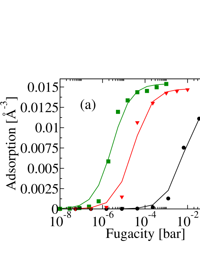
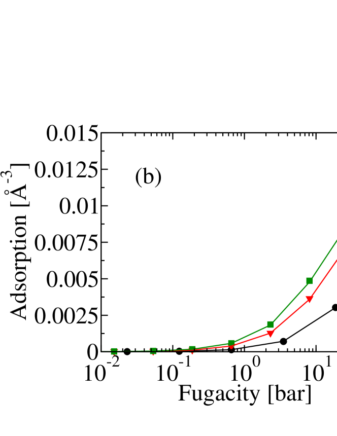
The difference between the potential and kinetic energies of the various isotopes confined within the slit pore already indicates that a strong isotope effect is to be expected upon adsorption. In fact the the adsorption isotherms reported in Fig. 4 show that this is indeed the case.

The isotherms have been calculated using the PIGCMC technique and using, for all the isotopes, the same number of beads $P$ as in the simulation of adsorption within carbon nanotubes. For each pressure we have performed $2.5\times 10^{5}$ PIGCMC steps for equilibration, followed by $5\times 10^{5}$ steps for production. The lateral dimensions of the pore were such that in saturation condition, at least 300 particles were present in the simulation box, resulting in a size of about $L=70$ Å.

The computed isotherms for the three isotopes at $T=20$ K have a similar shape, though they are separated by two or three orders of magnitude in pressure; the heaviest specie is adsorbed at lower pressures than the lightest one. Moreover the saturation density is markedly different for the three isotopes, with T₂ having the largest and H₂ the smallest. The isotope effect is also sizeable for the adsorption at $T=77$ K, though not as significant as it is at the lowest temperature. The adsorption isotherms plotted in Fig. 4 are in good quantitative agreement with analogous computer simulation results already appeared in the literature. Wang and Johnson (1998); Kowalczyk et al. (2006)

Mixture	Temperature (K)	Zero pressure selectivity
T2/H2	20	1263
T2/H2	77	4.3
D2/H2	20	151
D2/H2	77	2.8

Table 4: Zero pressure selectivities of hydrogen mixtures in the $H=5.7$ Å slit pore

Calculation of the selectivity confirms the presence of a significant isotope effect. The zero pressure selectivities, shown in Table 4, are found to be quite high at low temperature, reaching a value of around $1200$ for the case of T₂/H₂ mixtures and being of the order of $150$ for D₂/H₂ mixtures. The selectivity has a very strong dependence on the temperature, and drops to values around $4$ and $3$ for T₂/H₂ and D₂/H₂ mixtures, respectively, at a temperature of $T=77$ K. Kowalczyk et al. (2007)

It is interesting to notice that the values of the zero pressure selectivity calculated for the narrow slit pores, although lower than the ones of the narrowest carbon nanotubes, are nonetheless larger than those one could expect on the basis of geometrical considerations, given the 2D confining nature of the carbon nanotubes and the 1D confining nature of slit pores. In fact, if one assumes that the two confining directions are independent the single particle partition function can be written as the product of the partition functions corresponding to the two degrees of freedom. As a consequence of Eq. (24), then, the selectivity could be written as the product of two contributions, one for each confining direction. Therefore the selectivity of the nanotube should be equal to the square of the selectivity of the slit pore, if the two systems have the same confinement property along each confining direction.

Figure 5: Selectivity for hydrogen isotope mixtures as a function of pressure in the $H=5.7$ Å slit pore at $T=20$ K. The upper panel shows the selectivity of a T₂/H₂ mixture ($y_{\rm T_{2}}=8\times 10^{-4}$), and the lower panel the selectivity of a D₂/H₂ mixture ($y_{\rm D_{2}}=7\times 10^{-3}$). The horizontal dashed lines correspond to the zero pressure values, reported in Tab. 4.

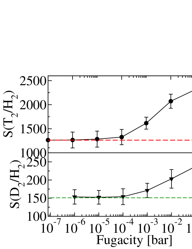
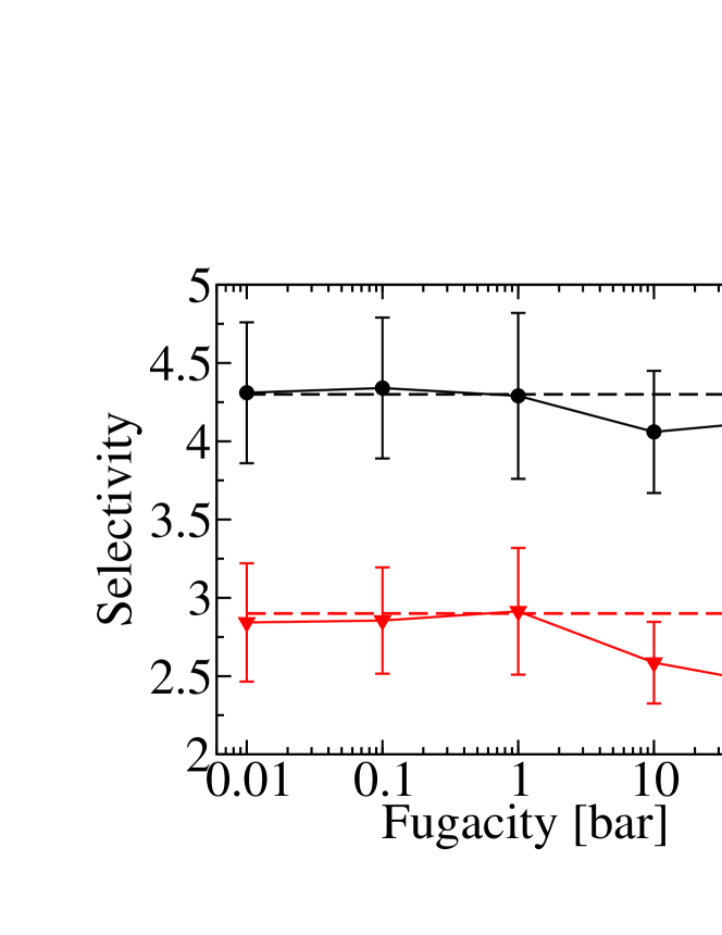
We have calculated the selectivity as a function of pressure for adsorption of hydrogen isotopes in slit pores using the Boltzmann bias method. We show in Fig. (5) and (6) the results obtained at the temperature of $T=20$ K and $T=77$ K respectively. The calculations at each pressure have been performed by simulating the adsorption of mixtures using the Boltzmann bias path integral grand canonical method and calculating the finite pressure selectivity directly from its definition, Eq. (23). For each state point a number between $1.5\times 10^{5}$ and $5\times 10^{5}$ of Monte Carlo steps were performed for the equilibration phase (depending on the pressure) and twice as many steps for the production run. In order to have an almost equal number of particles for both species within the simulation cell, we set the bulk mole fractions for the isotopes to the values indicated in the figures’ caption.

The results for $T=20$ K are qualitatively similar to what has already been observed for strongly confining nanotubes: Challa et al. (2002); Garberoglio and Johnson (2007) the selectivity rises from its zero pressure value for both tritium/hydrogen and deuterium/hydrogen mixtures, almost doubling its zero pressure value. This is consistent with the mechanism outlined above in the case of carbon nanotubes. Upon reaching saturation each adsorbed particle is confined also in the $xy$ plane and one would expect the selectivity to raise by a factor corresponding to the square of what is observed in the case of nanotubes. Since the selectivity increases by a factor of 1.4 in the case of nanotubes, one expects the selectivity in the slit pores to increase by a factor of $1.4\times 1.4\simeq 2$, as is indeed observed from the simulation result at $T=20$ K.

At the higher temperature of $T=77$ K the pressure dependence of the selectivity is less dramatic. One can see from Fig. 6 that the selectivity remains almost constant over four decades in pressure, possibly showing a slight tendency to decrease from its zero pressure value, as is particularly evident in the case of the deuterium/hydrogen mixture. In this case the further confinement along the $xy$ plane is less efficient than at low temperature, and the selectivity remains almost constant.

Figure 6: Selectivity for hydrogen isotope mixtures as a function of pressure in the $H=5.7$ Å slit pore at $T=77$ K. The circles shows the selectivity of a T₂/H₂ mixture ($y_{\rm T_{2}}=0.23$), and triangles the selectivity of a T₂/H₂ mixture ($y_{\rm D_{2}}=0.35$) as a function of the external pressure. The horizontal dashed lines correspond to the zero pressure values, reported in Tab. 4.

V Conclusions

We have developed an efficient method for the insertion/deletion moves of ring polymers in path integral grand canonical Monte Carlo simulations of fluids adsorbed in strongly confining geometries. In this case the kinetic energy of the adsorbed phase is larger than the thermal kinetic energy of a perfect gas at the same temperature and the standard procedure of inserting ring polymers configuration drawn from the ideal gas distribution is highly inefficient because the polymers are on average too large to fit within the narrow channels, resulting in a very low acceptance ratios. The new algorithm presented here is based on the idea of taking ring polymer configurations from a canonical simulation of independent particles already adsorbed.

The efficiency of the method comes from the fact that one uses as insertion candidates ring polymers already equilibrated according to the confining solid-fluid potential. We have observed an increase of the acceptance ratio for insertion moves up to 2 order of magnitudes when compared with the standard practice of trying to insert ideal gas ring polymer configurations, and a corresponding decrease of the time needed to perform a simulation.

The algorithm has been validated by calculating adsorption isotherms of pure fluids within narrow carbon nanotubes and graphite slit pores and comparing them with results already published in the literature, or obtained by us using the standard algorithm. Moreover we have calculated the pressure dependence of the isotopic selectivity in narrow nanotubes and slit pores and showed that even in the case of very strong confinement its value increases from the zero pressure limit.

Although this method becomes progressively inefficient near saturation conditions, its simplicity, effectiveness and ease of programming makes it a suitable candidate for simulating adsorption of quantum gases under conditions of strong confinement in a wide range of loadings.

Finally we would like to point out that this simulation technique can be applied to classical simulation of adsorption of small molecules or polymers within narrow channels. Ganazzoli and Raffaini (2005)

Appendix A Probability distribution for ring polymer configuration

The partition function of a free particle is

$$Z=\int d^{3}x_{1}~{}\langle x_{1}|\exp(-\beta p^{2}/2m)|x_{1}\rangle=\frac{V}{\Lambda^{3}}$$ (26)

that becomes, after a Trotter expansion,

$$Z=\int d^{3}x_{1}d^{3}x_{2}\ldots d^{3}x_{P}~{}\langle x_{1}|\exp(-\beta p^{2}/2mP)|x_{2}\rangle\ldots\langle x_{P}|\exp(-\beta p^{2}/2mP)|x_{1}\rangle$$ (27)

The integral can be rewritten using the variables defined in Eq. (19) together with the definition $\Delta r_{P}=-\displaystyle\sum_{i=1}^{P-1}\Delta r_{i}=x_{1}-x_{P}$,

$$Z=\left(\frac{P^{3/2}}{\Lambda^{3}}\right)^{P}\int d^{3}r_{1}d^{3}\Delta r_{1}\ldots d^{3}\Delta r_{P-1}\exp\left[-\frac{K}{2}\left(\Delta r_{1}^{2}+\Delta r_{2}^{2}+\ldots+\Delta r_{P-1}^{2}+\Delta r_{P}^{2}\right)\right]=\frac{V}{\Lambda^{3}}$$ (28)

where $K=2\pi P/\Lambda^{2}$. Since the integrand does not depend on $r_{1}$ on can integrate it obtaining

$$1=\Lambda^{3}\left(\frac{P^{3/2}}{\Lambda^{3}}\right)^{P}\int d^{3}\Delta r_{1}\ldots d^{3}\Delta r_{P-1}\exp\left[-\frac{K}{2}\left(\Delta r_{1}^{2}+\Delta r_{2}^{2}+\ldots+\Delta r_{P-1}^{2}+\Delta r_{P}^{2}\right)\right]$$ (29)

which can be interpreted as the normalization condition on the probability of observing a ring polymer of $P$ beads with separation from the neighboring beads equal to $\Delta r_{1}\ldots\Delta r_{P-1}$, the last one being fixed by the condition of having a closed ring polymer. Hence the probability for such a configuration is

$$F_{\mathrm{ring}}(\Delta r_{1},\ldots,\Delta r_{P-1})=\Lambda^{3}\left(\frac{P^{3/2}}{\Lambda^{3}}\right)^{P}\exp\left[-\frac{K}{2}\left(\Delta r_{1}^{2}+\Delta r_{2}^{2}+\ldots+\Delta r_{P-1}^{2}+\Delta r_{P}^{2}\right)\right]$$ (30)

References

- Allen and Tildesley (1989) M. Allen and D. Tildesley, Computer simulation of liquids (Oxford University Press, Oxford, 1989).
- Landau and Binder (2000) D. Landau and K. Binder, A guide to Monte Carlo simulations in statistical physics (Cambridge University Press, 2000), chap. 8.
- Wang et al. (1997) Q. Wang, J. Johnson, and J. Broughton, J. Chem. Phys. 107, 5108 (1997).
- Kowalczyk et al. (2007) P. Kowalczyk, P. Gauden, A. Terzyk, and S. Bhatia, Langmuir 23, 3666 (2007).
- Katorski and White (1964) A. Katorski and D. White, J. Chem. Phys. 40, 3183 (1964).
- Moiseyev (1975) N. Moiseyev, J. Chem. Soc. Faraday Trans. 1 71, 1830 (1975).
- Beenakker et al. (1995) J. Beenakker, V. Borman, and S. Krylov, Chem. Phys. Lett. 232, 379 (1995).
- Wang et al. (1999) Q. Wang, S. Challa, D. Sholl, and J. Johnson, Phys. Rev. Lett. 82, 956 (1999).
- Challa et al. (2001) S. Challa, D. Sholl, and J. Johnson, Phys. Rev. B 63, 245419 (2001).
- Challa et al. (2002) S. Challa, D. Sholl, and J. Johnson, J. Chem. Phys. 116, 814 (2002).
- Hathorn et al. (2001) B. Hathorn, B. Sumpter, and D. Noid, Phys. Rev. A 64, 022903 (2001).
- Trasca et al. (2003) R. Trasca, M. Kostov, and M. Cole, Phys. Rev. B 67, 035410 (2003).
- Lu et al. (2006) T. Lu, E. Goldfield, and S. Gray, J. Phys. Chem. B 110, 1742 (2006).
- Garberoglio et al. (2006) G. Garberoglio, M. DeKlavon, and J. Johnson, J. Phys. Chem. B 110, 1733 (2006).
- Hattori et al. (2006) Y. Hattori, H. Tanaka, F. Okino, H. Touhara, Y. Nakahigashi, S. Utsumi, H. Kanoh, and K. Kaneko, J. Phys. Chem. B 110, 9764 (2006).
- Bondarenko and Alekseev (2007) S. Bondarenko and I. Alekseev, in Hydrogen Materials Science and Chemistry of Carbon Nanomaterials, edited by T. Veziroglu (Springer Netherlands, 2007), vol. 3/2006 of NATO Security through Science Series, p. 493.
- Garberoglio and Johnson (2007) G. Garberoglio and J. K. Johnson, Preprint (2007), http://arxiv.org/abs/cond-mat/0703287.
- Feynman (1998) R. Feynman, Statistical Mechanics: A Set of Lectures (Perseus Books Group, 1998), 2nd ed.
- Ceperley (1995) D. Ceperley, Rev. Mod. Phys. 67, 279 (1995).
- Duane et al. (1987) S. Duane, A. Kennedy, B. Pendleton, and D. Roweth, Phys. Lett. B 195, 216 (1987).
- Fosdick and Jordan (1966) L. Fosdick and H. Jordan, Phys. Rev. 143, 58 (1966).
- (22) M. LaBrosse, private communication.
- Stan and Cole (1998) G. Stan and M. Cole, J. Low Temp. Phys. 110, 539 (1998).
- Zhang et al. (2004) X. Zhang, W. Wang, and G. Jiang, Fluid Phase Eq. 218, 239 (2004).
- Buch (1994) V. Buch, J. Chem. Phys. 100, 7610 (1994).
- Steele (1978) W. Steele, J. Phys. Chem. 82, 817 (1978).
- Sridhar et al. (2007) S. Sridhar, B. Smitha, and T. Aminabhavi, Separation & Purification Reviews 36, 113 (2007).
- Saufi and Ismail (2004) S. Saufi and A. Ismail, Carbon 42, 241 (2004).
- Wang and Johnson (1998) Q. Wang and J. Johnson, Mol. Phys. 95, 299 (1998).
- Kowalczyk et al. (2006) P. Kowalczyk, R. Holyst, A. Terzyk, and P. Gauden, Langmuir 22, 1970 (2006).
- Ganazzoli and Raffaini (2005) F. Ganazzoli and G. Raffaini, Phys. Chem. Chem. Phys 7, 3651 (2005).