Modeling an efficient Brownian heat engine

Abstract

We discuss the effect of subdividing the ratchet potential on the performance of a tiny Brownian heat engine that is modeled as a Brownian particle hopping in a viscous medium in a sawtooth potential (with or without load) assisted by alternately placed hot and cold heat baths along its path. We show that the velocity, the efficiency and the coefficient of performance of the refrigerator maximize when the sawtooth potential is subdivided into series of smaller connected barrier series. When the engine operates quasistatically, we analytically show that the efficiency of the engine can not approach the Carnot efficiency and, the coefficient of performance of the refrigerator is always less than the Carnot refrigerator due to the irreversible heat flow via the kinetic energy.

I Introduction

Brownian heat engine functions as transducer of thermal energy into mechanical work. It rectifies thermal fluctuations into a unidirectional current as long as the system is out of equilibrium. In the last few decades, the study of such a tiny engine has got considerable attention not only for the construction of a miniaturized engine that can help us to utilize energy resources at microscopic scales ph ; r but also for better understanding of the nonequilibrium statistical physics ken ; gom . The thermodynamic property of Brownian heat engine has been explored intensively by considering different model systems. Brownian heat engine working due to spatially-variable temperature is one of the model systems which has been studied in the pioneering works by Büttiker butt87 , Van Kampen kampen88 , and Landauer land88 . After the work of Büttiker, the ratchet model has been the subject of several authors miki3 ; Aus1 ; Ast2 ; bq ; mesfin1 ; mesfin2 . Recently, we considered an exactly solvable model of the heat engine and investigated the conditions under which the model works as a heat engine, as a refrigerator and as neither of the two mesfin3 . Not only we exposed the energetics of such an engine at a quasistatic limit but we also found the thermodynamic properties of the engine when it operates at a finite time.

In modeling of Brownian heat engine, one crucial but unexplored issue is the way how to maximize the velocity, the efficiency and the coefficient of performance of the refrigerator. For instance, in construction of artificial Brownian motors, one may need to design an engine that accomplishes its task as fast as possible and efficiently. The Brownian heat engine operates autonomously ken . The performance of this engine (how fast and efficiently can it achieve its task?) relies upon the way how the ingredients of the system are arranged prior to the engine operation. The purpose of this theoretical work is to present one possible way of improving the performance of the heat engine. Earlier, the mean first passage time (MFPT) of a Brownian particle that walks over rugged sawtooth potential was studied by us mesfin4 and in the work m1 ; m2 using super symmetric potential approach and using properties of random walk on networks formulated by Goldhirch and Gefen g1 ; g2 . The sawtooth potential was systematically subdivided into series of barriers without altering the barrier height, the potential width and the area under the barrier. The theoretical works revealed the existence of an optimal barrier subdivision that minimizes the MFPT. In this work, we use similar approach and study the effect of subdividing the ratchet potential on the performance of the engine. We show that the velocity, the efficiency and the coefficient of performance of the refrigerator tend to increase as the ratchet potential is subdivided into series of barriers.

Unlike macroscopic heat engines, the Carnot efficiency is unattainable for Brownian heat engines when the engines work quasistatically because of the irreversible heat flow via the kinetic energy ken ; Aus1 . In this work, we obtain a simple analytic expression for the efficiency at quasistatic limit. The analytic result reveals that the efficiency of the engine never goes to the Carnot efficiency at quasistatic limit. Another important but unexplored issue is the influence of the heat flow via the kinetic energy on the coefficient of performance of the refrigerator. In the present work, we analytically show that the coefficient of performance of the refrigerator is always less than the Carnot refrigerator when the engine operates quasistatically.

The paper is organized as follows: In section II, we present the model. In section III, we study the dependence of the efficiency and the velocity on the model parameters in the absence of external force. We show that the velocity and the efficiency attain optimum values at a particular value of barrier subdivision $N$. At qausistatic limit, the efficiency never goes to Carnot efficiency for any $N$ as the heat transfer via the kinetic energy is irreversible. In section IV, we consider the model in the presence of external load. We find that the velocity, the efficiency and the coefficient of performance of the refrigerator attain maximum values when the sawtooth potential is subdivided into series of smaller connected barrier series. We also show that the efficiency of the engine never approaches the Carnot efficiency and, the coefficient of performance of the refrigerator is always less than the Carnot refrigerator at quasistatic limit. Section V deals with summary and conclusion.

II The model

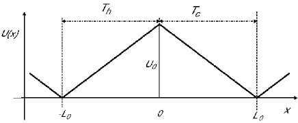
Consider a Brownian particle which walks in a viscous medium in a periodic sawtooth potential whose potential profile (see Fig. 1) is described by

$$U(x)=\cases{U_{0}[{x\over L_{0}}+1],&if $-L_{0}<x\leq 0$;\cr U_{0}[{-x\over L_{0}}+1],&if $0<x\leq L_{0};$\cr}$$ (1)

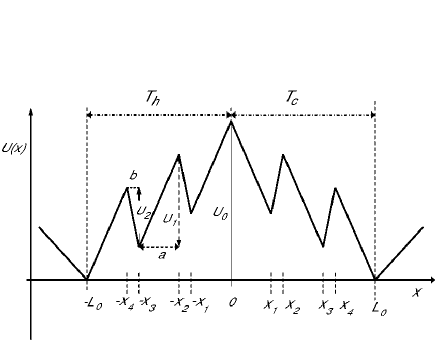
where $U_{0}$ and $L_{0}$ denote the barrier height and the width of the sawtooth potential, respectively. The viscous medium is alternatively in contact with the hot $T_{h}$ and the cold $T_{c}$ reservoirs along the reaction coordinate as shown in Fig. 1. Using the same theoretical frame work m1 , the sawtooth potential is subdivided into series of smaller connected barrier series. For example, Fig. 2 shows the left and the right sides of the sawtooth potential shown in Fig. 1 are subdivided into three small steps $N=3$. For single barrier step between $x_{2}$ and $x_{4}$, for simplicity, we choose $U_{1}=2U_{2}$ and $a=2b$ where $x_{4}-x_{2}=a+b$. In general, for $N$ equally spaced intervals, from the top of the barrier to either side, $L_{0}$ and $U_{0}$ are given by $L_{0}=Na+(N-1)b$ and $U_{0}=NU_{1}-(N-1)U_{2}$. Such parameterization is physically reasonable as the barrier height, the barrier width and the area under the barrier remain approximately constant as $N$ is varied mesfin4 ; m1 .

Figure 1: Periodic sawtooth potential without load when the number of barrier subdivisions $N=1$. The sawtooth potential is coupled with the hot $T_{h}$ and the cold $T_{c}$ reservoirs.

Figure 2: Periodic rugged potential without load for $N=3$. The potential is coupled with the hot $T_{h}$ and the cold $T_{c}$ reservoirs.

The Brownian particle attains a directional motion when it is exposed to the potential coupled with spatially variable temperature. For such a system, the general expression for the steady state current $J$ for the Brownian particle in any periodic potential with or without load is reported in the work mesfin3 . The closed form expression for the steady state current $J$ (please refer Appendix A, ref. mesfin3 ) is given by

$$J={-F\over G_{1}G_{2}+HF}.$$ (2)

The drift velocity $v$ of the particle is associated to the steady state current $J$ and it is given by $v=2JL_{0}$.

The hot reservoir is the ultimate source of energy for the engine. When the engine works as a heat engine, the net flux of the particle is from hot to the cold heat baths. Hence when the particle moves from the hot to the cold heat baths, for any $N$, the particle takes $U_{0}+v\gamma L_{0}+fL_{0}$ amount of energy from the hot reservoir to surmount the potential of magnitude $U_{0}$ and to overcome the viscous drag force $v\gamma$ as well as the external force of amount $f$. On the other hand, $1/2k_{B}(T_{h}-T_{c})$ amount of energy is transferred from the hot to the cold heat baths via kinetic energy Aus1 when the particle walks from the hot to the cold heat baths. Hence the Brownian particle takes

$$Q_{h}=(U_{0}+fL_{0}+\gamma vL_{0})+{1\over 2}k_{B}(T_{h}-T_{c})$$ (3)

amount of heat from the hot reservoir. The heat flow to the cold reservoir is given by

$$Q_{c}=U_{0}-L_{0}(f+\gamma v)+{1\over 2}k_{B}(T_{h}-T_{c}).$$ (4)

When the engine acts as refrigerator, the net flow of the particle is from the cold to the hot reservoirs. Note that, due to the particle recrossing between the hot and the cold reservoirs, heat is leaking from the hot to the cold reservoir of magnitude $1/2k_{B}(T_{h}-T_{c})$. This is in opposite direction to the heat being taken out of the cold reservoir. Hence, this quantity contributes as negative to $Q_{c}$. Thus, the net heat flow out of the cold reservoir is given by $Q_{c}=U_{0}-L_{0}(f+\gamma v)-{1\over 2}k_{B}(T_{h}-T_{c})$.

Not all motors are designed to pull loads and alternative proposals for efficiency depend on the task each motor performs. Some motors may have to achieve high velocity against a frictional drag. This basically implies that the objective of the motor is to move a certain distance in a given time interval. For such motors ($f=0$), the useful work is the difference between $Q_{h}$ and $Q_{c}$: $W=Q_{h}-Q_{c}=2\gamma vL_{0}$. For motors designed to pull loads $f\neq 0$, the useful work is given by $W=2fL_{0}$. The efficiency $\eta$ and the coefficient of performance (COP) of the refrigerator $P_{ref}$ of the engine is given by $\eta=W/Q_{h}$ and $P_{ref}=Q_{c}/W$.

The purpose of this theoretical work, for given parameter values of $U_{0}$ and $L_{0}$, to find the velocity, $v$, the efficiency, $\eta$, and the coefficient of performance of the refrigerator, $COP$, for various values of barrier subdivision, $N$. Next, the energetics of the Brownian heat engine will be explored as a function of model parameters both in the absence and in the presence of external force.

III The efficiency and the velocity in the absence of external force

In the absence of the external force $f=0$, the analytically obtained steady state current for $N=1$ is given by

$$J={1\over 2\gamma(T_{h}+T_{c})}({U_{0}\over L_{0}})^{2}\left({1\over e^{U_{0}\over T_{h}}-1}-{1\over e^{U_{0}\over T_{c}}-1}\right)$$ (5)

where $\gamma$ denotes the coefficient of friction of the Brownian particle. The magnitude of the coefficient of friction of the Brownian particle $\gamma$ depends on temperature of the viscous medium. As approximation, it is considered to be a constant. In Appendixes A and B, the expressions for $F$, $G_{1}$, $G_{2},$ and $H$ are given for $N=2$ and $N=3$, respectively. For $N\geq 4$, the expressions for $F$, $G_{1}$, $G_{2},$ and $H$ are lengthy and will not be presented in this work.

When one omits the heat exchange via kinetic energy (neglecting the term $1/2k_{B}(T_{h}-T_{c})$ in (3) and (4)), the efficiency goes to Carnot efficiency $\eta_{c}$ at quasistatic limit. The quasistatic limit of the engine is obtained when $U_{0}$ goes to zero. For any $N$, we explore the efficiency at quasistatic limit and find that $\displaystyle\lim_{{U_{0}\to 0}}{\eta}=(T_{h}-T_{c})/T_{h},$ which is exactly equal to the efficiency of the Carnot engine.

Figure 3: The drift velocity $v$ versus the potential barrier $u$ for values $\tau$=2 and $\ell$=$1$. In the limit $u\to 0$ and $u\to\infty$, the velocity $v\to 0$. $v$ increases with the number of barrier subdivisions. The velocity $v$ attains maximum values at a particular value of $u$. The potential $u$, at which the velocity of the particle is maximum, shifts to wards the left as the number of barrier subdivisions increase

Figure 4: The efficiency $\eta$ as a function of the barrier height $u$ for parameter values of $\tau$=2 and $\ell$=$1$. In the limit $u\to 0$, $\eta_{rev}\to 2/3$ which is equal to the Carnot efficiency for the given parameter values. In the limit $u\to 0$, $\eta_{irr}\to 0$. When $u\to\infty$, $\eta\to 0$.

Figure 5: The plot of $\alpha$ as a function of $u$ for parameter values of $\tau$=1.5 and $\ell$=$1$. $\alpha$ is increasing function of $u$. For $u<29$, $\alpha_{4}>\alpha_{2}$, $\alpha_{3}$,…$\alpha_{10}$. This implies $N=N_{op}=4$ is the optimal value of barrier subdivision. On other hand, when $u>29$, $N=N_{op}=6$ is the optimal value of barrier subdivision.

The heat flow via the kinetic energy significantly affects the efficiency of the Brownian heat engines. Next, considering the heat flow via the potential and the kinetic energies, we explore the thermodynamic property of the engine. Let us introduce dimensionless parameters before exploring the dependence of the velocity and the efficiency on different values of barrier subdivision $N$. We introduce scaled parameters: scaled length $\ell=1$, scaled barrier height $u=U_{0}/k_{B}T_{c}$, scaled current $j=J/J_{0}$ where $J_{0}=k_{B}T_{c}/\gamma L_{0}^{2}$, scaled velocity $v=2j/\ell$ and scaled temperature $\tau={T_{h}\over T_{c}}-1$. Here $k_{B}$ denotes Boltzmann’s constant. For simplicity, it is considered to be unity. We also introduce dimensionless parameters $\alpha_{i}=\eta_{i}/\eta_{1}$ ($i=2,3$, $...$ $N$) where $\eta_{i}$ and $\eta_{1}$ are the efficiencies when $N=i$ and $N=1$, respectively.

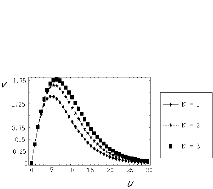
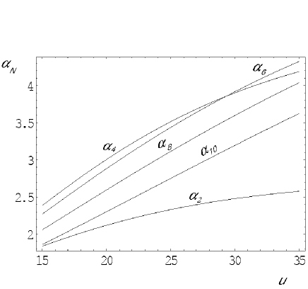
The dependence of the steady state current or equivalently the drift velocity on the potential $u$ can be analyzed by exploiting the analytically obtained steady state current (for instance, see Eq. (5) for the case $N=1$ and, the expressions shown in the Appendixes A and B for the cases $N=2$ and 3, respectively). The directional current is the result of spatial temperature difference along the ratchet potential. In the absence of the ratchet potential, the average velocity of the particle is zero, i.e.; the velocity $v$ vanishes when $u\to 0$ (see Fig. 3). In the limit $u\to\infty$, $j\to 0$ as the particle encounters a difficulty of jumping the high potential barrier of the ratchet potential, see Fig. 3. The velocity $v$ attains maximum value at a particular value of $u$. Note that the engine operates with maximum power at this particular value of $u$. The potential $u$, at which the velocity of the particle is maximum, shifts to wards the right as the number of barrier subdivisions increase as it can be readily seen in Fig. 3. Note that in the system we consider, the left and the right sides of the sawtooth potential are coupled with the hot and the cold baths, respectively. For such a system, positive velocity exhibits that the net flux of the particle is from the hot to the cold reservoirs and the engine operates only as a heat engine. Figure 3 shows that the velocity is positive for any $N$.

For high potential barriers, the Brownian particle encounters a difficulty of jumping the sawtooth potential when the background temperature is weak. Subdividing the barrier along the reaction coordinates enables the Brownian particle to cross each small barrier with small thermal kicks and ultimately the particle crosses the high potential barrier within short period of time than the time taken by the particle when it crosses the smooth potential barrier. Hence subdividing the sawtooth potential enhances the drift velocity $v$ as depicted in Fig. 3. The possibility of enhancing the escape rate of a Brownian particle over sawtooth potential under specific conditions was envisaged m1 ; m2 . The analytical finding revealed that the escape rate of the Brownian particle is enhanced for subdivided reaction coordinate which qualitatively agrees with this work.

Figure 6: The drift velocity $v$ versus $\tau$ for values of $u$=24 and $\ell$=$1$. In the limit $\tau\to 0$ (since $T_{h}=T_{c}$, the system is in thermal equilibrium), the steady state current $j$ vanishes: $j\to 0$. The drift velocity $v$ intensifies as $\tau$ and $N$ increase.

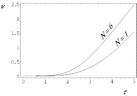
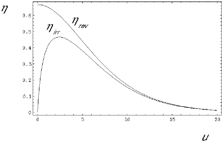
The analytically determined efficiency $\eta$ is plotted as a function of $u$ in Fig. 4 for the case $N=1$. When one considers the heat flow via the potential energy, in the limit $u\to 0$, $\eta_{rev}\to 2/3$ which is equal to the Carnot efficiency for parameter values of $\tau$=2 and $\ell$=$1$. On the other when we consider the heat flow both via the potential and the kinetic energies, $\eta_{irr}\to 0$ when $u\to 0$ and $u\to\infty$. This exhibits that quasistatic process may not be the best working condition for the Brownian heat engines which agrees with the claim of Hondou and Sekimoto ken . In addition, $\eta_{irr}$ attains a maximum value at finite value of $u$. The same figure depicts that $\eta_{irr}<\eta_{rev}$ and $\eta_{irr,rev}\to 0$ when $u\to\infty$.

The plot of $\alpha$ as a function of $u$ is displayed in Fig. 5. The enhancement in the efficiency is high when $\tau$ is small. For $u<29$, $\alpha_{4}>\alpha_{2}$, $\alpha_{3}$,…$\alpha_{10}$. This implies $N=N_{op}=4$ is the optimal value of barrier subdivision, at which the efficiency (velocity) is maximum, for a given parameter values. Note that the optimal barrier subdivision $N_{op}$ is sensitive to the choices of model parameters. For instance when $u>29$, $N=N_{op}=6$ is the optimal value of barrier subdivision.

The net flux of the particle strictly depends on the temperature difference between the hot and the cold baths. In the limit $\tau\to 0$ (since $T_{h}=T_{c}$, the system is in thermal equilibrium), the steady state current $j$ vanishes, i.e.; $j\to 0$ (see Eq. (5) for the case $N=1$ and the expressions shown in the Appendixes A and B for the cases $N=2$ and 3, respectively). The unidirectional current $j$ is due to the non homogenous temperature profile along the ratchet potential as the particle in the hot bath can easily crosses the potential barrier of the sawtooth potential than the particle in the cold bath. When the magnitude of the rescaled temperature $\tau$ steps up, the tendency of the particle in the hot bath to reach the top of the ratchet potential hill increases than the particle in the cold reservoir. This leads to an increase in the current $j$ or the drift velocity $v$ as shown in Fig. 6. The same figure shows that the net flux of the particle intensifies with $N$. The plot of $\alpha$ as a function of $\tau$ is displayed in Fig. 7. Significant enhancement of the efficiency is observed when $\tau$ is small.

Figure 7: The plot of $\alpha$ as a function of $\tau$ for values of $u$=24 and $\ell$=$1$.

IV The efficiency, the velocity and the performance of the refrigerator in the presence of external force

In the presence of external force, the net flow of the particle depends on the magnitude of the external force. For large load, current reversal may occur and this indicates that the engine operates not only as a heat engine but also as a refrigerator. In the presence of constant external force $f$, similar to the previous section, the closed form expression for steady state is given by $J={-F/(G_{1}G_{2}+HF)}.$ For $N=1$, the expressions for $F$, $G_{1}$, $G_{2},$ and $H$ are given by

$$F = e^{a-b}-1,$$

$$G_{1} = \frac{L_{0}}{aT_{h}}\left(1-e^{-a}\right)+\frac{L_{0}}{bT_{c}}e^{-a}\left(e^{b}-1\right),$$

$$G_{2} = \frac{\gamma L_{0}}{a}\left(e^{a}-1\right)+\frac{\gamma L_{0}}{b}e^{a}\left(1-e^{-b}\right).$$ (6)

On the other hand, $H=A+B+C$, where

$$A = \frac{\gamma}{T_{h}}\left(\frac{L_{0}}{a}\right)^{2}(a+e^{-a}-1),$$

$$B = \frac{\gamma L_{0}L_{0}}{abT_{c}}(1-e^{-a})(e^{b}-1),$$

$$C = \frac{\gamma}{T_{c}}\left(\frac{L_{0}}{b}\right)^{2}(e^{b}-1-b).$$ (7)

Here $a=(U_{0}+fL_{0})/T_{h}$ and $b=(U_{0}-fL_{0})/T_{c}$. The expressions for $N\geq 2$ are lengthy and will not be presented in this work. The drift velocity $v$ is related to the steady state current and it is given by $v=2JL_{0}$. Introducing additional rescaled parameter: $\lambda=fL_{1}/T_{c}$, we study how the velocity, the efficiency and the coefficient of performance of the refrigerator behave as $N$ varies.

Figure 8: The drift velocity $v$ versus the rescaled load $\lambda$ for values $u=12$, $\ell=1$ and $\tau=1$. For $\lambda<4$, the net particle flow is from the hot to the cold reservoirs. The drift velocity $v=0$ when $\lambda=4$. Current inversion occurs when $\lambda>4$.

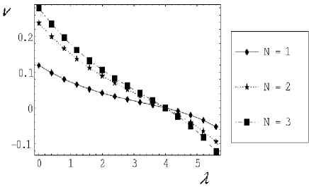
Figure 8 presents the plot of the velocity $v$ versus rescaled load $\lambda$ for $N=1$, $2$ and $3$. As shown in the figure for $\lambda<4$, the load is not strong enough to reverse the direction of the net flux of the particle, i.e., the net flow of the particle is from the hot to the cold reservoirs and hence the model works as a heat engine. On other hand for $\lambda>4$, the current becomes negative and the model acts as a refrigerator. The particle velocity is zero at $\lambda=4$. In general, for any number of barrier subdivisions $N$ the velocity $v=0$, when the load is

$$f_{0}={\tau U_{0}\over(\tau+2)L_{0}}.$$ (8)

When one omits the heat exchange via kinetic energy (neglecting the term $1/2k_{B}(T_{h}-T_{c})$ in (3) and (4)), for any $N$, in the quasistatic limit $v^{+}\to 0$, the efficiency is equal to Carnot efficiency:

$$\lim_{v^{+}\to 0}{\eta_{C}}={T_{h}-T_{c}\over T_{h}}$$ (9)

and in the quasistatic limit $v^{-}\to 0$, the coefficient of performance of the refrigerator is equal to Carnot refrigerator:

$$\lim_{v^{-}\to 0}{P_{ref}}={T_{c}\over T_{h}-T_{c}}.$$ (10)

We further investigate the thermodynamic property of the engine by including the heat exchange via the kinetic and the potential energies. At a quasistatic limit, for any $N$, the efficiency takes a simple form:

$$\lim_{v^{+}\to 0}\eta_{irr}^{*}={T_{h}-T_{c}\over T_{h}}\delta=\eta_{c}\delta$$ (11)

where

$$\delta={2U_{0}\over{2U_{0}T_{h}\over T_{c}}+0.5{T_{h}^{2}\over T_{c}}-0.5T_{c}}.$$ (12)

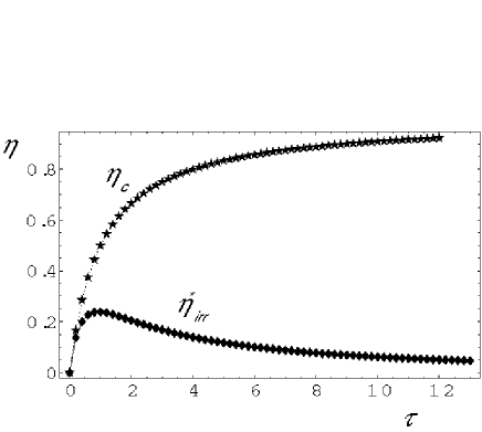
Note that $\delta<1$ when $T_{h}>T_{c}$. This exhibits that the efficiency of the engine never approaches the Carnot efficiency at quasistatic limit as there is irreversible heat transfer via the kinetic energy from the hot to the cold heat baths. The unattainability of the Carnot efficiency, at a quasistatic limit, was reported in the work ken by solving the Kramers equation at the stall force. Exploiting the analytical expressions (9) and (11), one can explore how $\eta_{irr}^{*}$ and $\eta_{C}$ behave as a function of $\tau$ as displayed in Fig. 9. The figure shows that in the limit $T_{h}\to T_{c}$, $\eta_{irr}^{*}\to\eta_{C}$ while $\eta_{irr}^{*}\ll\eta_{C}$ when $T_{c}\ll T_{h}$. This exhibits that the heat transfer via the kinetic energy is considerable when $\tau$ steps up.

Figure 9: The efficiency $\eta$ versus $\tau$ when the engine works quasistatically. $\eta_{C}$ denotes the Carnot efficiency while $\eta_{irr}^{*}$ denotes the efficiency of the irreversible heat engine when it operates quasistatically for fixed $u=2$.

Figure 10: The coefficient of performance of the refrigerator $P_{ref}$ versus $\tau$ when the heat engine works quasistatically. $P_{rec}^{C}$ denotes the Carnot refrigerator while $P_{irr}^{*}$ denotes $P_{ref}$ of the irreversible heat engine when it operates quasistatically for fixed $u=8$.

In the limit $v^{-}\to 0$, the coefficient of performance of the refrigerator converges to

$$\lim_{v^{-}\to 0}{P_{ref}}={T_{c}\over T_{h}-T_{c}}\Delta.$$ (13)

where

$$\Delta={U_{0}{T_{c}\over T_{h}}-0.25{T_{h}^{2}\over T_{c}}+0.25T_{c}\over U_{0}}.$$ (14)

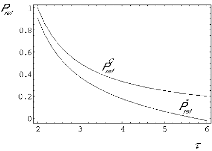
When $T_{h}>T_{c}$ and within the region where the model works as a refrigerator, $\Delta<1$. This reveals that the coefficient of performance of the refrigerator $P_{ref}$ is always less than the Carnot refrigerator at a quasistatic limit. The quasistatic behavior of the engine can be explored by exploiting the analytic expressions (10) and (13) as shown in Fig. 10. The figure depicts that $P_{ref}^{*}<P_{ref}^{C}$ and, in the limit $T_{h}\to T_{c}$, $P_{ref}^{*}\to P_{ref}^{C}$.

Figure 11: The drift velocity $v$ as a function of rescaled temperature $\tau$ for fixed parameters $u=10$, $\ell=1$ and $\lambda=2.0$. For $\tau<0.5$, the velocity $v$ takes negative values and the engine works as a refrigerator within this region. At $\tau=0.5$, the velocity $v=0$ while when $\tau>0.5$, the net particle current is from the hot to the cold reservoirs. As shown in the figure, $|v|$ intensifies as the number of barrier subdivisions increase.

Figure 12: The coefficient of performance of the refrigerator $P_{ref}$ versus $\tau$ (for reversible case) for fixed $u=10$, $\ell=1$ and $\lambda=2.0$. $P_{ref}$ is a decreasing function of $\tau$ and it rises up with $N$. In the limit $\tau\to 0.5$, $P_{ref}\to 2$ which is equal to the Carnot refrigerator for the given parameter values.

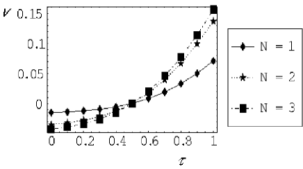
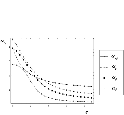
We next explore how $v$ and $P_{ref}$ behave as a function of $\tau$ for $N=1$, 2 and 3. The dependence of the velocity $v$ on the rescaled temperature $\tau$ is demonstrated in Fig. 11 for $N=$1, 2 and 3. As shown in the Fig. 11, when $\tau<0.5$, the load is strong enough to reverse the net particle flow and the velocity is negative. On other hand, when $\tau=0.5$, the temperature renormalizes the effect of the load and $v=0$. For $\tau>0.5$, the temperature gains strength to overcome the load and hence the current is positive in this region. Within the region where the model works as a heat engine, $v$ strengthens with $N$ and $\tau$. In the region where the model works as a refrigerator, $|v|$ intensifies as $N$ increases as shown in Fig. 11. This is because subdividing the sawtooth potential into small barriers enables the Brownian particle to cross these small barriers at small thermal kicks. On the other hand, when $\tau$ is small, the background thermal kick is weak for the particle to cross the smooth sawtooth potential barrier.

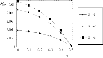
Figure 12 depicts the plot of $P_{ref}$ versus $\tau$. The coefficient of performance of the refrigerator $P_{ref}$ is a decreasing function of $\tau$ and it attends a maximum value when $N$ steps up. When the rescaled temperature $\tau$ increases, $P_{ref}$ declines towards the Carnot refrigerator.

V Summary and conclusion

In this work, we consider a model of Brownian heat engine. The dependence of the velocity, the efficiency and the coefficient of performance of the refrigerator is investigated for different number of barrier subdivisions, $N$. We show that the velocity and the efficiency attain optimum values at a particular value of barrier subdivision $N$. In the presence of external load we find that the velocity, the efficiency and the coefficient of performance of the refrigerator attain maximum values when the sawtooth potential is subdivided into series of smaller connected barrier series.

Considering the heat exchange via the potential and the kinetic energies, we show that Carnot efficiency is unachievable for Brownian heat engines when the engines work quasistatically. Quasistatic consideration for the Brownian heat engines also reveals that the coefficient of performance of the refrigerator is always less than the Carnot refrigerator.

In this work, considering an exactly solvable model, we explore the energetics of a Brownian heat engine not only at quasistatic limit but also at any finite time. This theoretical work suggests that the performance of the heat engine can be improved by subdividing the sawtooth potential into series of small barrier steps systematically by considering physically reasonable parameterization.

Appendix A

In this Appendix we will give the expressions for $F$, $G_{1}$, $G_{2}$ and $H$ which define the value of the steady state current, $J^{L}$, for zero external load case when $N=2$.

$$F = e^{{-U_{0}\over T_{c}}+{U_{0}\over T_{h}}}-1,$$ (A1)

$$G_{1} = {3L_{0}\over 5U_{0}}e^{-U_{0}\over T_{h}}[-2-2e^{U_{0}\over 3T_{C}}+2e^{2U_{0}\over 3T_{C}}+e^{U_{0}\over T_{C}}-2e^{U_{0}\over 3T_{h}}+2e^{2U_{0}\over 3T_{h}}]+{3L_{0}\over 5U_{0}},$$ (A2)

$$G_{2} = {L_{0}\gamma\over 5U_{0}}(-3e^{({1\over T_{h}}-{1\over T_{C}})U_{0}}T_{C}-3T_{h}-6e^{U_{0}\over 3T_{h}}T_{h}+6e^{2U_{0}\over 3T_{h}}T_{h})+$$ (A3)

$${3L_{0}\gamma\over 5U_{0}}e^{{-2U_{0}\over 3T_{C}}+{U_{0}\over T_{h}}}[-6T_{C}+6e^{U_{0}\over 3T_{C}}T_{C}+3e^{2U_{0}\over 3T_{c}}(T_{C}+T_{h})],$$

$$H^{L} = T_{1}(T_{2}+T_{3}+T_{4}+T_{5}+T_{6}),$$ (A4)

$$T_{1} = {L_{0}^{2}\gamma\over 25T_{h}U_{0}^{2}}e^{-{1\over 3}({1\over T_{C}}+{3\over T_{h}})U_{0}},$$ (A5)

$$T_{2} = 36e^{U_{0}\over T_{h}}T_{C}T_{h}+18e^{U_{0}\over 3T_{C}}T_{h}^{2}+18e^{2U_{0}\over 3T_{C}}T_{h}^{2}-18e^{U_{0}\over 3_{C}}T_{h}^{2}-9e^{4U_{0}\over 3T_{C}}T_{h}^{2},$$ (A6)

$$T_{3} = -36e^{{1\over 3}({3\over T_{C}}+{1\over T_{h}})U_{0}}T_{h}^{2}+45e^{(T_{C}+T_{h})U_{0}\over 3T_{C}T{h}}T_{h}^{2}-36e^{2(T_{C}+T_{h})U_{0}\over 3T_{C}T{h}}T_{h}^{2},$$ (A7)

$$T_{4} = 54e^{2(T_{C}+T_{h})U_{0}\over 3T_{C}T{h}}T_{h}^{2}+36e^{(4T_{C}+T_{h})U_{0}\over 3T_{C}T{h}}T_{h}^{2}+18e^{2(T_{C}+2T_{h})U_{0}\over 3T_{C}T{h}}T_{h}^{2}+$$ (A8)

$$36e^{(T_{C}+2T_{h})U_{0}\over 3T_{C}T{h}}T_{h}^{2},$$

$$T_{5} = -18e^{(T_{C}+4T_{h})U_{0}\over 3T_{C}T{h}}T_{h}^{2}+36e^{{U_{0}\over T_{C}}+{2U_{0}\over 3T_{h}}}T_{h}^{2}+9e^{{4U_{0}\over 3T_{C}}+{U_{0}\over T_{h}}}(T_{h}(T_{h}+T_{C}),$$ (A9)

$$T_{6} = 18e^{(T_{C}+T_{h})U_{0}\over T_{C}T{h}}T_{h}(2T_{C}+T_{h})-18e^{{2U_{0}\over 3T_{C}}+{U_{0}\over T_{h}}}T_{h}(2T_{C}+T_{h})+$$ (A10)

$$e^{{U_{0}\over 3T_{C}}+{U_{0}\over T_{h}}}(-45T_{h}(T_{C}+T_{h})-6T_{h}U_{0}+2U_{0}^{2}).$$

Appendix B

In this Appendix we will give the expressions for $F$, $G_{1}$, $G_{2}$ and $H$ which define the value of the steady state current, $J$, for zero external load case when $N=3$.

$$F = e^{{-U_{0}\over T_{c}}+{U_{0}\over T_{h}}}-1,$$ (B1)

$$G_{1} = {L_{0}e^{-U_{0}\over T_{h}}\over 2U_{0}}(-2-2e^{U_{0}\over 4T_{C}}+2e^{3U_{0}\over 4T_{C}}+e^{U_{0}\over T_{C}}-2e^{U_{0}\over 4T_{h}}+2e^{3U_{0}\over 4T_{h}}+e^{U_{0}\over T_{h}}),$$ (B2)

$$G_{2} = {-L_{0}\gamma\over 2U_{0}}(e^{U_{0}({1\over T_{h}}-{1\over T_{C}})}T_{C}+2e^{{U_{0}\over T_{h}}-{3U_{0}\over 4T_{C}}}T_{C}-2e^{{U_{0}\over T_{h}}-{U_{0}\over 4T_{C}}}T_{C})+$$ (B3)

$${-L_{0}\gamma\over 2U_{0}}(T_{h}+2e^{U_{0}\over 4T_{h}}T_{h}-2e^{3U_{0}\over 4T_{h}}T_{h}-e^{U_{0}\over T_{h}}(T_{h}+T_{C})),$$

$$H = T_{1}+T_{2}(T_{3}+T_{4}),$$ (B4)

$$T_{1} = {L_{0}^{2}\gamma T_{C}\over 4U_{0}^{2}}(-5+8e^{-U_{0}\over 4T_{C}}-12e^{U_{0}\over 4T_{C}}+4e^{U_{0}\over 2T_{C}}+4e^{3U_{0}\over 4T_{C}}+e^{U_{0}\over T_{C}}),$$ (B5)

$$T_{2} = {L_{0}^{2}\gamma T_{h}\over 4U_{0}^{2}}(e^{U_{0}\over 2T_{h}}-1)e^{-U_{0}\over T_{h}},$$ (B6)

$$T_{3} = (-2-2e^{U_{0}\over 4T_{C}}+2e^{3U_{0}\over 4T_{C}}+e^{U_{0}\over T_{C}}+e^{0.5U_{0}({2\over T_{c}}+{1\over T_{h}})},$$ (B7)

$$T_{4} = 2e^{0.25U_{0}({1\over T_{h}}+{4\over T_{C}})}+2e^{0.25U_{0}({2\over T_{h}}+{3\over T_{C}})}-6e^{U_{0}\over 4T_{h}}-6e^{U_{0}\over 2T_{h}}+8e^{3U_{0}\over 4T_{h}},$$ (B8)

$$T_{5} = -4e^{U_{0}(T_{h}+T_{C})\over 4T_{h}T_{C}}-2e^{U_{0}(T_{h}+2T_{C})\over 4T_{h}T_{C}}+4e^{U_{0}(3T_{h}+T_{C})\over 4T_{h}T_{C}}.$$ (B9)

References

- (1) R.D. Astumian, P. Hanggi, Phys. Today 55, 33 (2002).
- (2) P. Reimann, Phys. Rep. 361, 57 (2002).
- (3) Tsuyoshi Hondou and Ken Sekimoto, Phys. Rev. E 62, 6021 (2000).
- (4) A. Gomez-Marin and J.M. Sancho, Phys. Rev. E 74, 062102 (2006).
- (5) Büttiker M., Z. Phys. B 68, 161 (1987).
- (6) Van Kampen N. G., IBM J.Res. Dev. 32, 107 (1988).
- (7) Landauer R., J. Stat. Phys. 53, 233 (1988).
- (8) Miki Matsuo and Shin-ichi Sasa, Physica A 276, 188 (1999).
- (9) Derènyi I. and Astumian R. D., Phys. Rev. E 59, R6219 (1999).
- (10) Derènyi I., Bier M. and Astumian R. D., Phys. Rev. Lett 83, 903 (1999).
- (11) B.Q. Ai, H.Z. Xie, D.H. Wen, X.M. Liu, L.G. Liu, Eur. Phys. J. B 48, 101 (2005)
- (12) Mesfin Asfaw and Mulugeta Bekele, Eur. Phys. J. B 38, 457 (2004).
- (13) Mesfin Asfaw and Mulugeta Bekele, Phys. Rev. E 72, 056109 (2005).
- (14) Mesfin Asfaw and Mulugeta Bekele, Physica A 384, 346 (2007).
- (15) Mesfin Asfaw, Senior B.Sc. thesis, Addis Ababa University, Addis Ababa, (1999), (unpublished).
- (16) Mulugeta Bekele, G. Ananthakrishna and N. Kumar, Pramana - J. Phys. 46, 403 (1996).
- (17) Mulugeta Bekele, G. Ananthakrishna and N. Kumar, Physica A 270, 149 (1999).
- (18) I. Goldhirsch and Y. Gefen, Phys. Rev. A 33, 2583 (1986).
- (19) I. Goldhirsch and Y. Gefen, Phys. Rev. A 35, 1317 (1987).
- (20) J.M. Sancho, M. San Miguel, D. Dürr, J. Stat. Phys. 28, 291 (1982).