Counting lattice points in the moduli space of curves.

Abstract.

We show how to define and count lattice points in the moduli space $\mathcal{M}_{g,n}$ of genus $g$ curves with $n$ labeled points. This produces a polynomial with coefficients that include the Euler characteristic of the moduli space, and tautological intersection numbers on the compactified moduli space.

1. Introduction

Let $\mathcal{M}_{g,n}$ be the moduli space of genus $g$ curves with $n$ labeled points. The decorated moduli space $\mathcal{M}_{g,n}\times\mathbb{R}^{n}_{+}$ equips the labeled points with positive numbers $(b_{1},...,b_{n})$. It has a cell decomposition due to Penner, Harer, Mumford and Thurston

(1) $$\mathcal{M}_{g,n}\times\mathbb{R}^{n}_{+}\cong\bigcup_{\Gamma\in\mathcal{F}{\rm at}_{g,n}}P_{\Gamma}$$

where the indexing set $\mathcal{F}{\rm at}_{g,n}$ is the space of labeled fatgraphs of genus $g$ and $n$ boundary components. See Section 2 for definitions of a fatgraph $\Gamma$, its automorphism group $Aut\Gamma$ and the cell decomposition (1) realised as the space of labeled fatgraphs with metrics. Restricting this homeomorphism to a fixed $n$-tuple of positive numbers $(b_{1},...,b_{n})$ yields a space homeomorphic to $\mathcal{M}_{g,n}$ decomposed into compact convex polytopes $P_{\Gamma}(b_{1},...,b_{n})$. When the $b_{i}$ are positive integers the polytope $P_{\Gamma}(b_{1},...,b_{n})$ is an integral polytope and we define $N_{\Gamma}(b_{1},...,b_{n})$ to be its number of positive integer points. The weighted sum of $N_{\Gamma}$ over all labeled fatgraphs of genus $g$ and $n$ boundary components is the lattice count polynomial:

Definition 1.

$\quad\displaystyle N_{g,n}(b_{1},...,b_{n})=\sum_{\Gamma\in\mathcal{F}{\rm at}_{g,n}}\frac{1}{|Aut\Gamma|}N_{\Gamma}(b_{1},...,b_{n})$

Each integral point in the polytope $P_{\Gamma}(b_{1},...,b_{n})$ corresponds to a Dessin d’enfants defined by Grothendieck [3] which represents a curve in $\mathcal{M}_{g,n}$ defined over $\bar{\mathbb{Q}}$. Thus the lattice count polynomial $N_{g,n}(b_{1},...,b_{n})$ counts curves defined over $\bar{\mathbb{Q}}$. This is described in Section 2 where the integral points in $P_{\Gamma}(b_{1},...,b_{n})$ represent metrics on labeled fatgraphs with integer edge lengths, or equivalently curves equipped with a canonical meromorphic quadratic (Strebel) differential with integral residues.

Quite generally the number of integer points in a convex polytope is a piecewise defined polynomial. Nevertheless the following theorem shows that a weighted sum of the piecewise defined polynomials $N_{\Gamma}(b_{1},...,b_{n})$ is a polynomial.

Theorem 1.

The number of lattice points $N_{g,n}(b_{1},...,b_{n})$ is a degree $3g-3+n$ polynomial in the integers $(b_{1}^{2},...,b_{n}^{2})$ depending on the parity of the $b_{i}$.

The dependence on the parity means that $N_{g,n}(b_{1},...,b_{n})$ is represented by $2^{n}$ polynomials (by symmetry at most $[\frac{n}{2}]+2$ are different.) The polynomials are symmetric under permutations of $b_{i}$ of the same parity. If the number of odd $b_{i}$ is odd then $N_{g,n}(b_{1},...,b_{n})=0$. Otherwise, the top degree homogeneous part of $N_{g,n}(b_{1},...,b_{n})$ is independent of the parity. Table 1 shows the simplest polynomials. The factorisations are expected from the vanishing result of Lemma 2 in Section 2.3.

Table 1. Lattice count polynomials for even $b_{i}$

g	n	$N_{g,n}(b_{1},...,b_{n})$
0	3	1
1	1	$\frac{1}{48}\left(b_{1}^{2}-4\right)$
0	4	$\frac{1}{4}\left(b_{1}^{2}+b_{2}^{2}+b_{3}^{2}+b_{4}^{2}-4\right)$
1	2	$\frac{1}{384}\left(b_{1}^{2}+b_{2}^{2}-4\right)\left(b_{1}^{2}+b_{2}^{2}-8\right)$
2	1	$\frac{1}{2^{16}3^{3}5}\left(b_{1}^{2}-4\right)\left(b_{1}^{2}-16\right)\left(b_{1}^{2}-36\right)\left(5b_{1}^{2}-32\right)$

Harer and Zagier [5] calculated the orbifold Euler characteristic $\chi\left(\mathcal{M}_{g,1}\right)$ and Penner [10] calculated $\chi\left(\mathcal{M}_{g,n}\right)$ for general $n$. This information is encoded in the lattice count polynomial for all even $b_{i}$.

Theorem 2.

$N_{g,n}(0,...,0)=\chi\left(\mathcal{M}_{g,n}\right)$.

Kontsevich [6] defined the volume polynomial

$$V_{g,n}(b_{1},...,b_{n})=\sum_{\Gamma\in\mathcal{F}{\rm at}_{g,n}}\frac{1}{|Aut\Gamma|}Vol_{\Gamma}(b_{1},...,b_{n})$$

where $Vol_{\Gamma}(b_{1},...,b_{n})$ is the volume of the convex polytope $P_{\Gamma}(b_{1},...,b_{n})$. (The Laplace transform of $V_{g,n}$ appears as $I_{g}$ in [6].) He showed that the coefficients give intersection numbers of Chern classes of the tautological line bundles $L_{i}$ over the compactified moduli space $\overline{\mathcal{M}}_{g,n}$. By considering finer and finer meshes it follows that the homogeneous top degree part of the lattice point count polynomial is the volume polynomial.

Theorem 3.

$N_{g,n}(b_{1},...,b_{n})=V_{g,n}(b_{1},...,b_{n})+$ lower order terms.

Corollary 1.

For $|{\bf d}|=\sum_{i}d_{i}=3g-3+n$ and ${\bf d}!=\prod d_{i}!$ the coefficient $c_{\bf d}$ of $b^{2{\bf d}}=\prod b_{i}^{2d_{i}}$ in $N_{g,n}(b_{1},...,b_{n})$ is the intersection number

$$c_{\bf d}=\frac{1}{2^{6g-6+2n-g}{\bf d}!}\int_{\overline{\mathcal{M}}_{g,n}}c_{1}(L_{1})^{d_{1}}...c_{1}(L_{n})^{d_{n}}.$$

Kontsevich proved that these tautological intersection numbers satisfy a recursion relation conjectured by Witten [12] that determine the intersection numbers. The lattice count polynomials satisfy a recursion relation that uniquely determine the polynomials and when restricted to the top degree terms imply Witten’s recursion.

Theorem 4.

The lattice count polynomials satisfy the following recursion relation which determines the polynomials uniquely from $N_{0,3}$ and $N_{1,1}$.

(5) $$\left(\sum_{i=1}^{n}b_{i}\right)N_{g,n}(b_{1},...,b_{n}) = \sum_{i\neq j}\sum_{p+q=b_{i}+b_{j}}pqN_{g,n-1}(p,b_{1},..,\hat{b}_{i},..,\hat{b}_{j},..,b_{n})$$

$$+ \sum_{i}\sum_{p+q+r=b_{i}}pqr\biggl{[}N_{g-1,n+1}(p,q,b_{1},..,\hat{b}_{i},..,b_{n})$$

$$\hskip 56.9055pt+\sum_{\begin{array}[]{c}_{g_{1}+g_{2}=g}\\ _{I\sqcup J=\{1,..,\hat{i},..,n\}}\end{array}}N_{g_{1},|I|}(p,b_{I})N_{g_{2},|J|}(q,b_{J})\biggr{]}$$

The proof of Theorem 4 is elementary. The recursion relation (5) is used to prove Theorem 1. It resembles Mirzakhani’s recursion relation [7] between polynomials giving the Weil-Petersson volume of the moduli space. In fact the top homogeneous degree part of $N_{g,n}(b_{1},...,b_{n})$ coincides with the top homogeneous degree part of Mirzakhani’s Weil-Petersson volume polynomial (after multiplying by an appropriate power of $2$) since both of these coincide with Kontsevich’s volume. Mirzakhani [8] already showed the coefficients of the Weil-Petersson volume polynomial are the intersection numbers given in Corollary 1. Do and Safnuk [2] use fatgraphs to give a simpler proof of Mirzakhani’s recursion relation restricted to the top homogeneous degree part and show that it is a rescaled version of Mirzakhani’s proof.

Although Table 1 shows only even $b_{i}$, the recursion relation needs the odd cases too. We will fill in the cases of odd $b_{i}$ here. When $\sum b_{i}$ is odd, $N_{g,n}(b_{1},...,b_{n})\equiv 0$. The polynomial $N_{0,4}(b_{1},...,b_{4})$ is the same as in the table when $b_{1},...,b_{4}$ are all odd, and when exactly two of the $b_{i}$ are odd $N_{0,4}(b_{1},...,b_{4})=\frac{1}{4}\left(b_{1}^{2}+b_{2}^{2}+b_{3}^{2}+b_{4}^{2}-2\right)$. For genus 1 when $b_{1}$ and $b_{2}$ are odd $N_{1,2}(b_{1},b_{2})=\frac{1}{384}\left(b_{1}^{2}+b_{2}^{2}-2\right)\left(b_{1}^{2}+b_{2}^{2}-10\right)$.

Section 2 contains preliminaries on fatgraphs and lattice point counting. Theorems 1 and 4 are proven in Section 2.2. Section 2.3 contains a simple vanishing result for $N_{g,n}(b_{1},...,b_{2})$ which has powerful consequences. In Section 3 we prove Theorem 2 and treat the special case of $n=1$ labeled points.

Acknowledgements. The author would like to thank Norman Do for many useful conversations.

2. Fatgraphs

A fatgraph is a graph $\Gamma$ with vertices of valency $>2$ equipped with a cyclic ordering of edges at each vertex. In Figure 1 we use the projection to define the cyclic ordering to be anticlockwise at each vertex.

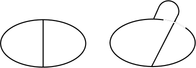
Figure 1. Fatgraphs

The two pictured fatgraphs are different, although the underlying graphs are the same. A fatgraph structure on a graph is equivalent to an embedding of a graph into a surface $\Gamma\to\Sigma$ such that $\Sigma-\Gamma$ is a union of disks. This gives a genus $g$ and number of boundary components $n$ to $\Gamma$. The examples in Figure 1 have genus 0 and 1 shown in Figure 2.

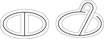
Figure 2. Graphs embedded in genus 0 and 1 surfaces

A labeled fatgraph is a fatgraph with boundary components labeled $1,...,n$. The set of all labeled fatgraphs of genus $g$ and $n$ boundary components is notated by $\mathcal{F}{\rm at}_{g,n}$.

It is useful to describe a fatgraph in the following equivalent way [6] which makes the automorphisms transparent. Given a graph $\Gamma$ with vertices of valency $>2$, let $X$ be the set of oriented edges, so each edge of $\Gamma$ appears in $X$ twice. Define the map $\tau_{1}:X\to X$ that flips the orientation of each edge. A fatgraph, or ribbon, structure on $\Gamma$ is a map $\tau_{0}:X\to X$ that permutes cyclically the oriented edges with a common source vertex. Let $X_{0}$, $X_{1}$ and $X_{2}$ be the vertices, edges and boundary components of the fatgraph $\Gamma$. Then $X_{0}=X/\tau_{0}$, $X_{1}=X/\tau_{1}$ and $X_{2}=X/\tau_{2}$ for $\tau_{2}=\tau_{0}\tau_{1}$. An automorphism of the labeled fatgraph $\Gamma$ is a permutation $\phi:X\to X$ that commutes with $\tau_{0}$ and $\tau_{1}$ and acts trivially on $X_{2}$. The examples in Figure 1 given any labeling have automorphism groups $\{1\}$ and $\mathbb{Z}_{6}$.

A metric on a labeled fatgraph $\Gamma$ assigns positive numbers—lengths—to each edge of the fatgraph. If $\Gamma\in\mathcal{F}{\rm at}_{g,n}$ then the valency $>2$ conditions on the vertices ensures that the number of edges $e(\Gamma)$ of $\Gamma$ is bounded $e(\Gamma)\leq 6g-6+3n$. Let $P_{\Gamma}$ be the $6g-6+3n$ cell consisting of all metrics on $\Gamma$. Construct the cell-complex

$$\mathcal{M}_{g,n}^{\rm combinatorial}=\bigcup_{\Gamma\in\mathcal{F}{\rm at}_{g,n}}P_{\Gamma}$$

where we identify isometric metrics on fatgraphs, and when the length of an edge $l_{E}\to 0$ we identify this with the metric on the fatgraph with the edge $E$ contracted. By the existence and uniqueness of meromorphic quadratic differentials with foliations having compact leaves, known as Strebel differentials, the cell complex is homeomorphic to the decorated moduli space $\mathcal{M}_{g,n}^{\rm combinatorial}\cong\mathcal{M}_{g,n}\times\mathbb{R}_{+}^{n}$ [4].

Denote by $P_{\Gamma}(b_{1},...,b_{n})\subset P_{\Gamma}$ the metrics on $\Gamma$ with fixed boundary lengths ${\bf b}=(b_{1},...,b_{n})\in\mathbb{R}_{+}^{n}$ or equivalently with specified residues of the (square root of the) associated Strebel differential. Then

(6) $$\mathcal{M}_{g,n}^{\rm combinatorial}(b_{1},...,b_{n})=\bigcup_{\Gamma\in\mathcal{F}{\rm at}_{g,n}}P_{\Gamma}(b_{1},...,b_{n})\cong\mathcal{M}_{g,n}.$$

2.1. Counting lattice points in convex polytopes

A convex polytope $P\subset\mathbb{R}^{n}$ can be defined as the convex hull of a finite set of vertices in $\mathbb{R}^{n}$. We will consider integral polytopes $P$ where the vertices lie in $\mathbb{Z}^{n}$. Define the number of integral points in $P$ by $N_{P}=\#\{P\cap\mathbb{Z}^{n}\}$ and $N_{P}(k)=\#\{kP\cap\mathbb{Z}^{n}\}$ where $kP$ rescales $\lambda_{j}\mapsto k\lambda_{j}$. Also, define $N^{0}_{P}(k)$ to be the number of integral points in the interior of $kP$.

Theorem 2.1 (Ehrhart).

If $P\subset\mathbb{R}^{n}$ is an $n$-dimensional convex polytope then

$$N_{P}(k)={\rm Vol}(P)k^{n}+...$$

is a degree $n$ polynomial in $k$ with top coefficient the volume of $P$. Furthermore,

$$N^{0}_{P}(k)=(-1)^{n}N_{P}(-k).$$

We can define a convex polytope with positive codimension as follows. Given a linear map $A:\mathbb{R}^{N}\to\mathbb{R}^{n}$ and ${\bf b}\in\mathbb{R}^{n}$ define

$$P_{A}({\bf b})=\{{\bf x}\in\mathbb{R}_{+}^{N}|A{\bf x}={\bf b}\}.$$

If $A$ and $b$ have integer entries (with respect to the standard bases) then $P_{A}({\bf b})$ is integral and we define $N_{P_{A}}({\bf b})=\#\{P_{A}\cap\mathbb{Z}^{N}\}$. In this case $N_{P_{A}}({\bf b})$ is a piecewise defined polynomial in $\bf b$ - for example, $N_{P_{A}}({\bf b})$ may be zero for some values of ${\bf b}$.

The set $P_{\Gamma}({\bf b})$ in (6) is a convex polytope defined by solutions ${\bf x}\in\mathbb{R}_{+}^{e(\Gamma)}$ of

$$A_{\Gamma}{\bf x}={\bf b}$$

where $A_{\Gamma}$ is the incidence matrix that maps the vector space generated by edges of $\Gamma$ to the vector space generated by boundary components of $\Gamma$—an edge maps to the sum of its two incident boundary components. In the examples in Figure 1 the incidence matrices are

$$A_{\Gamma}=\left(\begin{array}[]{ccc}1&1&0\\ 1&0&1\\ 0&1&1\end{array}\right),\quad A_{\Gamma^{\prime}}=\left(\begin{array}[]{ccc}2&2&2\end{array}\right).$$

We define

$$N_{\Gamma}({\bf b})=\#\{P_{A}\cap\mathbb{Z}_{+}^{N}\}.$$

It is natural to allow non-negative solutions although we allow only positive integer solutions. This is justified by the fact that if some of the $x_{i}$ vanish then this will be counted using a fatgraph obtained by collapsing edges of $\Gamma$. (If the collapsing of edges of $\Gamma$ does not yield a fatgraph, for example collapsing a loop, then we do not want to count such solutions.)

Since each edge is incident to exactly two (not necessarly distinct) boundary components the columns of $A_{\Gamma}$ add to 2, or equivalently $(1,1,...,1)\cdot A_{\Gamma}=(2,2,...,2)$. Thus,

$$\sum b_{i}=(1,1,...,1)\cdot{\bf b}=(1,1,...,1)\cdot A_{\Gamma}{\bf x}=(2,2,...,2)\cdot{\bf x}\in 2\mathbb{Z}$$

so $N_{\Gamma}({\bf b})=0$ if $\sum b_{i}$ is odd. Hence the lattice count polynomial $N_{g,n}(b_{1},...,b_{n})$ given in Definition 1 also vanishes when $\sum b_{i}$ is odd.

If we relax the condition on fatgraphs that the valency of each vertex must be $>2$ then Grothendieck [3] showed that fatgraphs with all edge lengths 1 possess branched covers of $\mathbb{P}^{1}$ branched over 0, 1 and $\infty$. By a theorem of Belyi these correspond to curves defined over $\bar{\mathbb{Q}}$. When the length of each edge is a positive integer this is the same as a string of length 1 edges joined by valency 2 vertices. Thus, $N_{g,n}(b_{1},...,b_{n})$ counts curves defined over $\bar{\mathbb{Q}}$ branched over of $0,1,\infty\in\mathbb{P}^{1}$ with all points over 1 of ramification 2, and all points over 0 of ramification $>2$.

For a convex polytope $P\subset\mathbb{R}^{N}$ and a polynomial $\phi$ on $\mathbb{R}^{N}$ define the following generalisation of counting lattice points.

$$N_{P}(\phi,k)=\sum_{{\bf x}\in kP\cap\mathbb{Z}^{N}}\phi({\bf x})$$

and $N^{0}_{P}(\phi,k)$ the sum over interior integer points of $kP$. Later when applying the recursion relation we will need to calculate sums with a parity restriction as in Lemma 1 because the polynomials $N_{g,n}$ vanish if the sum of the arguments is odd.

Lemma 1.

(7) $$S_{m}(k)=\sum_{\begin{array}[]{c}\scriptstyle p+q=k\\ \scriptstyle q{\rm\ even}\end{array}}p^{2m+1}q,\quad R_{m,m^{\prime}}(k)=\sum_{\begin{array}[]{c}\scriptstyle p+q+r=k\\ \scriptstyle r{\rm\ even}\end{array}}p^{2m+1}q^{2m^{\prime}+1}r$$

are odd polynomials in $k$ of degree $2m+3$, respectively $2m+2m^{\prime}+5$, depending on the parity of $k$.

Proof.

The dependence on the parity means that there are two polynomials $S^{\rm even}_{m}(k)$ and $S^{\rm odd}_{m}(k)$ depending on whether $k$ is even or odd. The same is true for $R_{m.m^{\prime}}(k)$. Notice that

$$S_{m}(k)=2N_{P}(\phi_{1},k)$$

for $P=\{(x,y)\in\mathbb{R}_{+}^{2}|x+2y=1\}$ and $\phi_{1}=x^{2m+1}y$ (substitute $q=2Q$.) Similarly,

$$R_{m,m^{\prime}}(k)=2N_{P^{\prime}}(\phi_{2},k)$$

for $P^{\prime}=\{(x,y,z)\in\mathbb{R}_{+}^{3}|x+y+2z=1\}$ and $\phi_{2}=x^{2m+1}y^{2m^{\prime}+1}z$.

The polytopes $P$ and $P^{\prime}$ are rational, not integral. They can be expressed in terms of the integral convex polytopes of higher dimension

$$P_{1}=\{x\geq 0,y\geq 0,x+2y\leq 2\},\quad P_{2}=\{x\geq 0,y\geq 0,z\geq 0,x+y+2z\leq 2\}.$$

For $k$ even

$$S^{\rm even}_{m}(k)=N_{P_{1}}(\phi_{1},\frac{k}{2})-N^{0}_{P_{1}}(\phi_{1},\frac{k}{2}),\quad R^{\rm even}_{m,m^{\prime}}(k)=N_{P_{2}}(\phi_{2},\frac{k}{2})-N^{0}_{P_{2}}(\phi_{2},\frac{k}{2}).$$

A generalisation [1] of Ehrhart’s theorem states that for a dimension $n$ integral convex polytope $P\subset\mathbb{R}^{n}$, $N_{P}(\phi,k)$ is a degree $\deg\phi+n$ polynomial in $k$ and

$$N^{0}_{P}(\phi,k)=(-1)^{\deg\phi+n}N_{P}(\phi,-k).$$

For the cases at hand, $\deg\phi+n$ is even so the right hand side is $N_{P}(\phi,-k)$ and $S^{\rm even}_{m}(k)$ and $R^{\rm even}_{m,m^{\prime}}(k)$ are odd polynomials in $k$ of degree $2m+3$, respectively $2m+2m^{\prime}+5$. For $k$ odd,

$$S^{\rm odd}_{m}(k)=N^{0}_{P_{1}}(\phi_{1},\frac{k+1}{2})-N_{P_{1}}(\phi_{1},\frac{k-1}{2})$$

and $R^{\rm odd}_{m,m^{\prime}}(k)$ is the same expression with $P_{2}$ in place of $P_{1}$. Once again $S^{\rm odd}_{m}(k)$ and $R^{\rm odd}_{m,m^{\prime}}(k)$ are odd polynomials in $k$ of degree $2m+3$, respectively $2m+2m^{\prime}+5$. ∎

2.2. Recursion

Proof of Theorem 4.

The lattice count polynomial $N_{g,n}(b_{1},...,b_{n})$ counts labeled fatgraphs with positive integer edge lengths which we call integer fatgraphs in $P_{\Gamma}(b_{1},...,b_{n})$. We can produce an integer fatgraph in $P_{\Gamma}(b_{1},...,b_{n})$ from simpler integer fatgraphs in the three ways shown in Figures 3, 4 and 5. Choose a graph in $P_{\Gamma^{\prime}}(p,b_{3},...,b_{n})$ and add an edge of length $q/2$ inside the boundary of length $p$ as in Figure 3 so that $p+q=b_{1}+b_{2}$.

Figure 3. $\Gamma$ is obtained from a simpler fatgraph by adding the broken line.

Similarly, attach an edge and a loop of total length $q/2$ inside the boundary of length $p$ as in Figure 4 so that $p+q=b_{1}+b_{2}$.

Figure 4. $\Gamma$ is obtained by adding a line and loop of total length $q/2$.

In both cases for each $\Gamma^{\prime}$ there are $p$ possible ways to attach the edge so this construction contributes $pN_{g,n-1}(p,b_{3},...,b_{n})$ to $N_{g,n}(b_{1},...,b_{n})$. However we have overcounted, particularly when we repeat this construction for any pair $b_{i}$ and $b_{j}$, since each integer fatgraph in $P_{\Gamma}(b_{1},...,b_{n})$ can be produced in many ways like this. To deal with this, we overcount even further by taking $pqN_{g,n-1}(p,b_{3},...,b_{n})$, i.e. taking each constructed fatgraph $q$ times. But now we see that for each edge that we attach of length $q/2$ we have overcounted $q$ times. If we were to use all of the edges of $\Gamma$ in this way then we would have overcounted by

$$\sum_{E\in\Gamma}l(E)=\sum_{i=1}^{n}b_{i}.$$

Indeed all of the edges of $\Gamma$ are used, exactly once, when we include one further construction of the integer fatgraph $\Gamma$.

Choose an integer fatgraph in $P_{\Gamma^{\prime}}(p,q,b_{2},...,b_{n})$ for $\Gamma^{\prime}\in\mathcal{F}{\rm at}_{g-1,n+1}$ or choose two integer fatgraphs in $P_{\Gamma_{1}}(p,b_{2},...,b_{j})$ and $P_{\Gamma_{2}}(q,b_{j+1},...,b_{n})$ for $\Gamma_{1}\in\mathcal{F}{\rm at}_{g_{1},j}$ and $\Gamma_{2}\in\mathcal{F}{\rm at}_{g_{2},n+1-j}$ where $g_{1}+g_{2}=g$ and attach an edge of length $r/2$ connecting these two boundary components as in Figure 5 so that $p+q+r=b_{1}$.

Figure 5. $\Gamma$ is obtained from a single fatgraph or two disjoint fatgraphs by adding the broken line.

In the diagram, the two boundary components of lengths $p$ and $q$ are part of a fatgraph that may or may not be connected. There are $pq$ possible ways to attach the edge so this construction contributes $pqN_{g-1,n+1}(p,q,b_{2},...,b_{n})$ and $pqN_{g_{1},j}(p,b_{2},...,b_{j})N_{g_{2},n+1-j}(q,b_{j+1},...,b_{n})$ to $N_{g,n}(b_{1},...,b_{n})$ and again we have overcounted. We overcount further by a factor of $r$ to get $pqrN_{g-1,n+1}(p,q,b_{2},...,b_{n})$ and $pqrN_{g_{1},j}(p,b_{2},...,b_{j})N_{g_{2},n+1-j}(q,b_{j+1},...,b_{n})$. We repeat this for each $g_{1}+g_{2}=g$ and $I\sqcup J=\{2,...n\}$ and then for each $b_{j}$ in place of $b_{1}$.

As previewed above, each edge of $\Gamma$ has been attached to construct $\Gamma$ and $N_{g,n}(b_{1},...,b_{n})$ has been overcounted $\sum_{i=1}^{n}b_{i}$ times yielding (5). ∎

Remark. The idea in the proof above to overcount by the length of each edge of the graph $\Gamma$ comes from the similar idea introduced by Mirzakhani [7] where she unfolds a function on Teichmüller space that sums to the analogue of $b_{1}$.

To apply the recursion we need to first calculate $N_{0,3}(b_{1},b_{2},b_{3})$ and $N_{1,1}(b_{1})$. There are seven labeled fatgraphs in $\mathcal{F}{\rm at}_{0,3}$ coming from three unlabeled fatgraphs. It is easy to see that $N_{0,3}(b_{1},b_{2},b_{3})=1$ if $b_{1}+b_{2}+b_{3}$ is even (and 0 otherwise.) This is because for each $(b_{1},b_{2},b_{3})$ there is exactly one of the seven labeled fatgraphs $\Gamma$ with a unique solution of $A_{\Gamma}{\bf x}={\bf b}$ while the other six labeled fatgraphs yield no solutions. For example, if $b_{1}>b_{2}+b_{3}$ then only the fatgraph $\Gamma$ with $A_{\Gamma}=\left(\begin{array}[]{ccc}2&1&1\\ 0&1&0\\ 0&0&1\end{array}\right)$ has a solution and that solution is unique.

To calculate $N_{1,1}(b_{1})$, note that $A_{\Gamma}=[2\quad 2\quad 2]$ or $[2\quad 2]$ for the 2-vertex and 1-vertex fatgraphs. Hence

$$N_{1,1}(b_{1})=a_{1}\binom{\frac{b_{1}}{2}-1}{2}+a_{2}\binom{\frac{b_{1}}{2}-1}{1}$$

where $a_{1}$ is the number of trivalent fatgraphs (weighted by automorphisms) and $a_{2}$ is the number of 1-vertex fatgraphs. The genus 1 graph $\Gamma$ from Figure 1 has $|Aut\Gamma|=6$ so $a_{1}=1/6$, and $a_{2}$ uses the genus 1 figure 8 fatgraph which has automorphism group $\mathbb{Z}_{4}$ hence $a_{2}=1/4$. Thus

$$N_{1,1}(b_{1})=\frac{1}{6}\binom{\frac{b_{1}}{2}-1}{2}+\frac{1}{4}\binom{\frac{b_{1}}{2}-1}{1}=\frac{1}{48}\left(b_{1}^{2}-4\right).$$

We can also calculate $N_{1,1}(b_{1})$ using a version of the recursion

$$b_{1}N_{1,1}(b_{1})=\frac{1}{2}\sum_{\begin{array}[]{c}p+q+p=b\\ b{\rm\ even}\end{array}}pq.$$

We will calculate $N_{0,4}[b_{1},b_{2},b_{3},b_{4}]$ to demonstrate the recursion relation and the parity issue.

$$\left(\sum_{i=1}^{4}b_{i}\right)N_{0,4}(b_{1},b_{2},b_{3},b_{4})=\sum_{i\neq j}\sum_{\begin{array}[]{c}\scriptstyle p+q=b_{i}+b_{j}\\ \scriptstyle q{\rm\ even}\end{array}}pq.$$

If all $b_{i}$ are even, or all $b_{i}$ are odd, then $b_{i}+b_{j}$ is always even so the sum is over $p$ and $q$ even. We have

$$S^{\rm even}_{0}(k)=\sum_{i\neq j}\sum_{\begin{array}[]{c}\scriptstyle p+q=k\\ \scriptstyle q{\rm\ even}\end{array}}pq=4\binom{\frac{k}{2}+1}{3}$$

so

$$\left(\sum_{i=1}^{4}b_{i}\right)N_{0,4}({\bf b})=\sum_{i\neq j}4\binom{\frac{b_{i}+b_{j}}{2}+1}{3}=\left(\sum_{i=1}^{4}b_{i}\right)\frac{1}{4}\left(b_{1}^{2}+b_{2}^{2}+b_{3}^{2}+b_{4}^{2}-4\right)$$

agreeing with Table 1. If $b_{1}$ and $b_{2}$ are odd and $b_{3}$ and $b_{4}$ are even then we need

$$S^{\rm odd}_{0}(k)=\sum_{i\neq j}\sum_{\begin{array}[]{c}\scriptstyle p+q=k\\ \scriptstyle q{\rm\ even}\end{array}}pq=\frac{1}{2}\binom{k+1}{3}$$

so

$$\left(\sum_{i=1}^{4}b_{i}\right)N_{0,4}({\bf b}) = \sum_{(i,j)=(1,2){\rm\ or\ }(3,4)}4\binom{\frac{b_{i}+b_{j}}{2}+1}{3}+\sum_{(i,j)\neq(1,2){\rm\ or\ }(3,4)}\frac{1}{2}\binom{b_{i}+b_{j}+1}{3}$$

$$= \left(\sum_{i=1}^{4}b_{i}\right)\frac{1}{4}\left(b_{1}^{2}+b_{2}^{2}+b_{3}^{2}+b_{4}^{2}-2\right)$$

so we see that the polynomial representatives of $N_{0,4}({\bf b})$ agree up to a constant term.

Proof of Theorem 1.

We can use the recursion (5) to prove that $N_{g,n}(b_{1},...,b_{n})$ is a polynomial of the right degree but to prove that it is a polynomial in $b_{i}^{2}$ we need a different recursion formula (11). For simplicity we use (11) to prove each part of Theorem 1.

(11) $$b_{1}N_{g,n}(b_{1},...,b_{n}) = \sum_{j>1}\frac{1}{2}\left(\sum_{p+q=b_{1}+b_{j}}pqN_{g,n-1}(p,b_{2},..,\hat{b}_{j},..,b_{n})\right.$$

$$\left.\quad\quad+\sum_{p+q=b_{1}-b_{j}}pqN_{g,n-1}(p,b_{2},..,\hat{b}_{j},..,b_{n})\right)$$

$$+ \sum_{p+q+r=b_{1}}pqr\biggl{[}N_{g-1,n+1}(p,q,b_{2},...,b_{n})$$

$$\hskip 56.9055pt+\sum_{\begin{array}[]{c}_{g_{1}+g_{2}=g}\\ _{I\sqcup J=\{2,...,n\}}\end{array}}N_{g_{1},|I|}(p,b_{I})N_{g_{2},|J|}(q,b_{J})\biggr{]}$$

This differs from the recursion formula (5) by breaking the symmetry around $b_{1}$. The sum over the term $p+q=b_{1}-b_{j}$ needs to be interpreted as follows. If $b_{1}-b_{j}>0$ it is read as written, whereas if $b_{1}-b_{j}<0$ then replace $b_{1}-b_{j}$ by $b_{j}-b_{1}$ and negate the sum. (This is not the same as sending $(p,q)$ to $(-p,-q)$.)

We will prove the recursion (11) below. Before that we will prove that given $N_{0,3}$ and $N_{1,1}$ then (11) determines polynomials $N^{\prime}_{g,n}(b_{1},...,b_{n})$ of degree $3g-3+n$ in $b_{i}^{2}$. By induction, the simpler polynomials are polynomials in $b_{i}^{2}$ so monomials on the right hand side of the recursion are of the form

$$S_{m}(k)=\sum_{\begin{array}[]{c}\scriptstyle p+q=k\\ \scriptstyle q{\rm\ even}\end{array}}p^{2m+1}q,\quad R_{m,m^{\prime}}(k)=\sum_{\begin{array}[]{c}\scriptstyle p+q+r=k\\ \scriptstyle r{\rm\ even}\end{array}}p^{2m+1}q^{2m^{\prime}+1}r$$

as in (7). In Lemma 1 it is proven that $S_{m}(k)$ and $R_{m,m^{\prime}}(k)$ are odd polynomials in $k$. In particular, $S_{m}(b_{1}-b_{j})=-S_{m}(b_{j}-b_{1})$ explaining the interpretation of the sum over $b_{1}-b_{j}<0$

The sums over $p+q+r=b_{1}$ yield terms which are odd in $b_{1}$ from $R_{m,m^{\prime}}(b_{1})$ and even in $b_{i}$ for $i>1$ hence $1/b_{1}$ times these terms is even in all $b_{i}^{2}$. The sums over $p+q=b_{1}+b_{j}$ and $p+q=b_{1}-b_{j}$ have the same summands so each monomial occurs with the same coefficient. Hence the terms involving $b_{1}$ are of the form $S_{m}(b_{1}+b_{j})+S_{m}(b_{1}-b_{j})$ and since $S_{m}$ is odd, this sum is odd in $b_{1}$ and even in $b_{j}$, and even in the all other $b_{i}$. Again $1/b_{1}$ times these terms is even in all $b_{i}^{2}$. Thus by induction the polynomials generated by the recursion relation (11) from $N_{0,3}$ and $N_{1,1}$ are polynomials in $b_{i}^{2}$.

We will now calculate the degree in $b_{i}^{2}$. By induction $\deg N_{g,n-1}=3g-3+n-1$ and by Lemma 2 $S_{m}(k)$ takes a term $p^{2m+1}q$ and produces a degree $2m+3$ polynomial, i.e. it increases the degree by 1. In this case $3g-3+n-1+1=3g-3+n$ as required. Similarly, by induction $\deg N_{g-1,n+1}=3g-3+n-2$ and $\deg N_{g_{1},|I|}N_{g_{2},|J|}=3g-3+n-2$. By Lemma 2 $R_{m,m^{\prime}}(k)$ increases the degree of its summand by 2. Since $3g-3+n-2+2=3g-3+n$ the result is proven by induction starting from the degrees of $N_{0,3}$ and $N_{1,1}$.

As above, write $N^{\prime}_{g,n}$ for the polynomials produced from the recursion (11). To prove the recursion (11) we use the fact that both (5) and (11) uniquely determine $N_{g,n}$ and $N^{\prime}_{g,n}$ respectively. It remains to show that (11) $\Rightarrow$ (5), hence $N_{g,n}$ and $N^{\prime}_{g,n}$ necessarily coincide.

Apply (11) to each $b_{i}$ to calculate $b_{i}N^{\prime}_{g,n}(b_{1},...,b_{n})$ and add.

$$\left(\sum_{i=1}^{n}b_{i}\right)N^{\prime}_{g,n}(b_{1},...,b_{n}) = \sum_{i\neq j}\sum_{p+q=b_{i}+b_{j}}pqN^{\prime}_{g,n-1}(p,b_{1},..,\hat{b}_{i},..,\hat{b}_{j},..,b_{n})$$

$$+ \sum_{i}\sum_{p+q+r=b_{i}}pqr\biggl{[}N^{\prime}_{g-1,n+1}(p,q,b_{1},..,\hat{b}_{i},..,b_{n})$$

$$\hskip 56.9055pt+\sum_{\begin{array}[]{c}_{g_{1}+g_{2}=g}\\ _{I\sqcup J=\{1,..,\hat{i},..,n\}}\end{array}}N^{\prime}_{g_{1},|I|}(p,b_{I})N^{\prime}_{g_{2},|J|}(q,b_{J})\biggr{]}$$

$$+ \Delta$$

where

$$\Delta=\sum_{i\neq j}\frac{1}{2}\left(\sum_{p+q=b_{i}-b_{j}}+\sum_{p+q=b_{j}-b_{i}}\right)pqN^{\prime}_{g,n-1}(p,b_{1},..,\hat{b}_{i},..,\hat{b}_{j},..,b_{n})=0$$

since the sums contain only canceling odd terms $S_{m}(b_{i}-b_{j})+S_{m}(b_{j}-b_{i})=0$.

Thus $N_{g,n}$ and $N^{\prime}_{g,n}$ satisfy the recursion relation (5) which uniquely determines them, hence

$$N_{g,n}=N^{\prime}_{g,n}$$

so it follows that $N_{g,n}$ satisfies the recursion (11). ∎

Remark. The top degree term of recursion (11) is a discrete version of the integration recursion for volume given by Do and Safnuk [2]. They show their recursion is a rescaled version of Mirzakhani’s recursion relation [7] which give the Virasoro relations among tautological classes [8].

2.3. Vanishing

Lemma 2.

If $\displaystyle\sum_{i=1}^{n}b_{i}<4g+2n$ then $N_{g,n}(b_{1},...,b_{n})=0$.

Proof.

A labeled fatgraph $\Gamma\in\mathcal{F}{\rm at}_{g,n}$ has at least one vertex and hence at least $2g+n$ edges since $\chi(\Gamma)=1-2g-n$. Since $N_{g,n}$ counts positive integers solutions of $A_{\Gamma}x=b$, each $x_{i}\geq 1$, thus $\sum x_{i}\geq 2g+n$. Each edge contributes twice to the boundary of $\Gamma$ so

$$\sum_{i=1}^{n}b_{i}=2\sum_{i=1}^{e(\Gamma)}x_{i}\geq 4g+2n$$

and the lemma follows. ∎

Lemma 2 can be used to get strong information about the lattice count polynomial. For example, $N_{1,1}(2)=0$ and since it is a polynomial in $b_{1}^{2}$ of degree 1 we get $N_{1,1}(b_{1})=c(b_{1}^{2}-4)$. The genus 2 case gives $N_{2,1}(2)=0=N_{2,1}(4)=N_{2,1}(6)$ hence

$$N_{2,1}(b_{1})=c_{1}(b_{1}^{2}-4)(b_{1}^{2}-16)(b_{1}^{2}-36)(b_{1}^{2}+c_{2}).$$

Although it is very difficult to calculate $N_{g,n}$ directly using fatgraphs, in the simplest cases it is calculable by extending the idea behind the vanishing Lemma 2. When $\displaystyle\sum_{i=1}^{n}b_{i}=4g+2n$ the argument in the proof of Lemma 2 shows that each $x_{i}=1$ so $N_{g,n}$ counts 1-vertex fatgraphs.

3. Euler characteristic

Using the cell decomposition (1), the orbifold Euler characteristic of the moduli space can be calculated via a sum over labeled fatgraphs. Expressing the sum as a Feynman expansion Penner [10] calculated the following.

$$\chi(\mathcal{M}_{g,n})=\sum_{\Gamma\in\mathcal{F}{\rm at}_{g,n}}\frac{(-1)^{e(\Gamma)-n}}{|Aut\Gamma|}=\left\{\begin{array}[]{ll}(-1)^{n-1}(n-3)!&g=0\\ (-1)^{n-1}\frac{(2g+n-3)!}{(2g-2)!}\zeta(1-2g)&g>0\end{array}\right.$$

The exponent is the dimension of the cell since $\dim P_{\Gamma}=e(\Gamma)-n$.

The lattice count polynomial gives another way to calculate the Euler characteristic via $N_{g,n}(0,...,0)=\chi\left(\mathcal{M}_{g,n}\right)$. We will prove this here.

Proof of Theorem 2..

Define

$$R_{g,n}(z)=\sum_{{\bf b}\in\mathbb{Z}_{+}^{n}}N_{g,n}(b_{1},...,b_{n})z^{b_{1}+...+b_{n}}.$$

It has the following properties:

1. $R_{g,n}(z)$ is a meromorphic function, holomorphic on $\bar{\mathbb{C}}-\{\pm 1\}$.

2. $R_{g,n}(0)=0$

3. $R_{g,n}(\infty)=(-1)^{n}N_{g,n}(0,...,0)$.

Recall that $N_{g,n}({\bf b})$ is represented by a collection of polynomials depending on the parity of $b_{i}$. By the symmetry of these polynomials we can set $R_{g,n}(z)=\sum_{k=0}^{n}\binom{n}{k}R^{(k)}_{g,n}(z)$ where $k=$ the number of odd $b_{i}$. The basic idea behind property (1) is that if $p(n)=\sum_{j=0}^{k}p_{j}n^{j}$ is a polynomial then

$$\sum_{n>0}p(n)z^{n}=\sum_{j=0}^{k}p_{j}\sum_{n>0}n^{j}z^{n}=\sum_{j=0}^{k}p_{j}\left(z\frac{d}{dz}\right)^{j}\frac{z}{1-z}$$

which is a meromorphic function with pole at $z=1$ and known behaviour at $z=0$ and $z=\infty$. If we restrict the parity of $n$ then

(13) $$\sum_{\begin{array}[]{c}n>0\\ n{\rm\ even}\end{array}}p(n)z^{n}=\sum_{j=0}^{k}p_{j}\left(z\frac{d}{dz}\right)^{j}\frac{z^{2}}{1-z^{2}},\sum_{\begin{array}[]{c}n>0\\ n{\rm\ odd}\end{array}}p(n)z^{n}=\sum_{j=0}^{k}p_{j}\left(z\frac{d}{dz}\right)^{j}\frac{z}{1-z^{2}}$$

which are both meromorphic functions with poles at $z=\pm 1$. Furthermore,

$$\left(z\frac{d}{dz}\right)^{j}\left.\frac{z^{2}}{1-z^{2}}\right|_{z=\infty}=\left\{\begin{array}[]{cl}-1&j=0\\ 0&j>0\end{array}\right.,\quad\left(z\frac{d}{dz}\right)^{j}\left.\frac{z}{1-z^{2}}\right|_{z=\infty}=0.$$

Each polynomial $N_{g,n}(b_{1},...,b_{n})$ is a sum of monomials of the form $\prod_{1}^{n}b_{i}^{2m_{i}}$ so $R^{(k)}_{g,n}(z)$ is a sum of finitely many series

$$R^{(k)}_{g,n}(z)=\sum_{\bf m}c_{\bf m}\sum_{\begin{array}[]{c}{\bf b}\in\mathbb{Z}_{+}^{n}\\ b_{i}{\rm\ odd\ }i\leq k\end{array}}b_{1}^{2m_{1}}...b_{n}^{2m_{n}}z^{b_{1}+...+b_{n}}$$

which consists of terms of the form

$$\sigma^{(k)}_{\bf m}(z)=\sum_{\begin{array}[]{c}{\bf b}\in\mathbb{Z}_{+}^{n}\\ b_{i}{\rm\ odd\ }i\leq k\end{array}}b_{1}^{2m_{1}}...b_{n}^{2m_{n}}z^{b_{1}+...+b_{n}}=\prod_{i=1}^{k}\sum_{\begin{array}[]{c}b_{i}>0\\ b_{i}{\rm\ odd}\end{array}}b_{i}^{2m_{i}}z^{b_{i}}\cdot\prod_{i=k+1}^{n}\sum_{\begin{array}[]{c}b_{i}>0\\ b_{i}{\rm\ even}\end{array}}b_{i}^{2m_{i}}z^{b_{i}}.$$

This is a finite product of meromorphic functions each with poles only at $z=\pm 1$ by (13). Furthermore, from the evaluation at $\infty$ of such functions, $\sigma^{(k)}_{\bf m}(\infty)=(-1)^{n}$ if ${\bf m}={\bf 0}$ and $k=0$ and it vanishes otherwise. Thus, $R_{g,n}(\infty)$ contains only one non-vanishing term, $R_{g,n}(\infty)=R^{(0)}_{g,n}(\infty)=(-1)^{n}N_{g,n}(0,...,0)$ where we evaluate using the polynomial $N_{g,n}$ that takes in all even $b_{i}$.

We have proven (1) and (3). Property (2) follows from the strict positivity of the $b_{i}$ and the convergence of the series which follows from the convergence of $1+z+z^{2}+...$ for $|z|<1$.

We can calculate $R_{g,n}(\infty)$ in another way. For a vector $v=(v_{1},...,v_{n})$ with $v_{i}\in\mathbb{Z}_{+}$ define (the semigroup homomorphism) $|v|=\sum_{i=1}^{n}v_{i}$. Recall that the incident matrix $A_{\Gamma}=[\alpha_{1},...,\alpha_{e(\Gamma)}]$ for $\alpha_{i}\in\mathbb{R}^{n}$ of a labeled fatgraph $\Gamma$ defines a convex polytope $A_{\Gamma}x={\bf b}$ and $N_{\Gamma}({\bf b})$ counts integral points $x\in\mathbb{Z}_{+}^{e(\Gamma)}$. Thus

$$R_{\Gamma}(z) = \sum_{{\bf b}\in\mathbb{Z}_{+}^{n}}N_{\Gamma}(b_{1},...,b_{n})z^{b_{1}+...+b_{n}}=\sum_{x\in\mathbb{Z}_{+}^{e(\Gamma)}}z^{|A_{\Gamma}x|}$$

$$= \sum_{x\in\mathbb{Z}_{+}^{e(\Gamma)}}z^{\sum_{i=1}^{e(\Gamma)}x_{i}|\alpha_{i}|}=\prod_{i=1}^{e(\Gamma)}\sum_{x_{i}\in\mathbb{Z}_{+}}z^{x_{i}|\alpha_{i}|}$$

$$= \prod_{i=1}^{e(\Gamma)}\frac{z^{|\alpha_{i}|}}{1-z^{|\alpha_{i}|}}$$

so $R_{\Gamma}(\infty)=(-1)^{e(\Gamma)}$ and

$$R_{g,n}(\infty)=\sum_{\Gamma\in\mathcal{F}{\rm at}_{g,n}}\frac{(-1)^{e(\Gamma)}}{|Aut\Gamma|}=(-1)^{n}\chi(\mathcal{M}_{g,n}).$$

Combining this with property (3) yields the theorem

$$N_{g,n}(0,...,0)=\chi(\mathcal{M}_{g,n}).$$

∎

3.1. Calculating $N_{g,1}$.

When $n=1$ there is a more direct proof of Theorem 2. For any $\Gamma\in\mathcal{F}{\rm at}_{g,1}$ the incidence matrix is $A_{\Gamma}=[2,2,...,2]$. The equation $Ax=b$ has $\binom{\frac{b}{2}-1}{e(\Gamma)-1}$ positive integral solutions. Hence

$$N_{g,1}(b)=c_{6g-3}^{(g)}\binom{\frac{b}{2}-1}{6g-4}+c_{6g-4}^{(g)}\binom{\frac{b}{2}-1}{6g-5}+..+c_{k}^{(g)}\binom{\frac{b}{2}-1}{k-1}+..+c_{2g}^{(g)}\binom{\frac{b}{2}-1}{2g-1}$$

where the coefficients are weighted counts of fatgraphs of genus $g$ with $n=1$ boundary component

$$c_{k}^{(g)}=\sum_{\begin{array}[]{c}\Gamma\in\mathcal{F}{\rm at}_{g,1}\\ e(\Gamma)=k\end{array}}\frac{1}{|Aut\Gamma|}.$$

The polynomial $\binom{\frac{b}{2}-1}{k}$ evaluates at $b=0$ to $(-1)^{k}$ which gives a direct proof that the Euler characteristic is given by evaluation at 0.

$$N_{g,1}(0)=\sum_{\Gamma\in\mathcal{F}{\rm at}_{g,1}}\frac{(-1)^{e(\Gamma)-1}}{|Aut\Gamma|}=\chi(\mathcal{M}_{g,1}).$$

When $n=1$ the weighted number of trivalent fatgraphs and 1-vertex fatgraphs are known [11].

$$c_{6g-3}^{(g)}=2\frac{1}{12^{g}}\frac{(6g-5)!}{g!(3g-3)!},\quad c_{2g}^{(g)}=\frac{(4g-1)!}{4^{g}(2g+1)!}$$

We can calculate $N_{2,1}(b)$ without using the recursion relation (except to deduce that $N_{2,1}(b)$ is a polynomial of degree $4$ in $b^{2}$) by applying Lemma 2 to get $N_{2,1}(b)=0$ for $b=2,4$ and 6. This leaves two unknown coefficients which can be calculated from any two of the three pieces of known information $c_{9}^{(2)}$, $c_{4}^{(2)}$ and $N_{2,1}(0)$.

$$N_{2,1}(b) = \frac{1}{2^{16}3^{3}5}\left(b^{2}-4\right)\left(b^{2}-16\right)\left(b^{2}-36\right)\left(5b^{2}-32\right)$$

$$= \textstyle\frac{35}{6}\binom{\frac{b}{2}-1}{8}+\frac{105}{4}\binom{\frac{b}{2}-1}{7}+\frac{93}{2}\binom{\frac{b}{2}-1}{6}+\frac{161}{4}\binom{\frac{b}{2}-1}{5}+\frac{84}{5}\binom{\frac{b}{2}-1}{4}+\frac{21}{8}\binom{\frac{b}{2}-1}{3}.$$

The polynomial $N_{2,1}(b)$ enables us to calculate the weighted counts of fatgraphs $c_{k}^{(2)}$. We can similarly calculate $N_{3,1}$ and hence deduce the weighted counts of fatgraphs.

$$N_{3,1}(b) = \textstyle\frac{1}{2^{25}3^{6}5^{2}7}(b^{2}-4)(b^{2}-16)(b^{2}-36)(b^{2}-64)(b^{2}-100)(5b^{4}-188b^{2}+1152)$$

$$= \textstyle\frac{5005}{3}\binom{\frac{b}{2}-1}{14}+\frac{25025}{2}\binom{\frac{b}{2}-1}{13}+41118\binom{\frac{b}{2}-1}{12}+\frac{929929}{12}\binom{\frac{b}{2}-1}{11}+\frac{183955}{2}\binom{\frac{b}{2}-1}{10}$$

$$\textstyle+\frac{283767}{4}\binom{\frac{b}{2}-1}{9}+\frac{317735}{9}\binom{\frac{b}{2}-1}{8}+10813\binom{\frac{b}{2}-1}{7}+\frac{25443}{14}\binom{\frac{b}{2}-1}{6}+\frac{495}{4}\binom{\frac{b}{2}-1}{5}.$$

References

• [1] Brion, Michel and Vergne, MichΓ©le Lattice points in simple polytopes. J. Amer. Math. Soc. 10 (1997), 371–392.
• [2] Do, Norman and Safnuk, Brad Hyperbolic rescaling and symplectic structures on moduli spaces of curves. Preprint.
• [3] Grothendieck, Alexandre Esquisse d’un Programme. London Math. Soc. Lecture Note Ser. 242, Geometric Galois actions, 1, 5-48, Cambridge Univ. Press, Cambridge, 1997.
• [4] Harer, John The virtual cohomological dimension of the mapping class group of an orientable surface. Invent. Math. 84 (1986), 157-176.
• [5] Harer, John and Zagier, Don The Euler characteristic of the moduli space of curves. Invent. Math. 85 (1986), 457-485.
• [6] Kontsevich, Maxim Intersection theory on the moduli space of curves and the matrix Airy function. Comm. Math. Phys. 147 (1992), 1-23.
• [7] Mirzakhani, Maryam Simple geodesics and Weil-Petersson volumes of moduli spaces of bordered Riemann surfaces. Invent. Math. 167 (2007), 179-222.
• [8] Mirzakhani, Maryam Weil-Petersson volumes and intersection theory on the moduli space of curves. J. Amer. Math. Soc., 20 (2007), 1-23.
• [9] Penner, R. C. The decorated TeichmΓΌller space of punctured surfaces. Comm. Math. Phys. 113 (1987), 299-339.
• [10] Penner, R. C. Perturbative series and the moduli space of Riemann surfaces. J. Diff. Geom. 27 (1988), 35-53.
• [11] Walsh, T.R.S. and Lehman, A.B. Counting rooted maps by genus. J. Combin. Theory Ser. B 13 (1972), 192-218.
• [12] Witten, Edward Two-dimensional gravity and intersection theory on moduli space. Surveys in differential geometry (Cambridge, MA, 1990), 243–310, Lehigh Univ., Bethlehem, PA, 1991.