The Inverse Simpson Paradox
(How to win without overtly cheating)

Abstract

Given two sets of data which lead to a similar statistical conclusion, the Simpson Paradox [10] describes the tactic of combining these two sets and achieving the opposite conclusion. Depending upon the given data, this may or may not succeed. Inverse Simpson is a method of decomposing a given set of comparison data into two disjoint sets and achieving the opposite conclusion for each one. This is always possible; however, the statistical significance of the conclusions does depend upon the details of the given data.

1 Introduction

Anyone contemplating a statistical analysis is warned, at an early stage of the game, “but don’t combine the statistics of monkey wrenches and watermelons”, or the equivalent. Failure to heed this instruction – at a more sophisticated level, to be sure – gives rise frequently to Simpson’s Paradox (here, in its 2-trial sequence version): if choice $A$ is “statistically better” than choice $B$ in each of two sets of trials under differing circumstances, then it may happen that merging the two sets of data produces the opposite conclusion. Consider the following specially constructed example for the sake of illustration:

Table 1: Simpson Paradox Prototype

	Trial #1	Trial #2	Total
$S_{A}\equiv$ $A$ successes	60	60	120
$F_{A}\equiv$ $A$ failures	20	140	160
$S_{B}\equiv$ $B$ successes	140	20	160
$F_{B}\equiv$ $B$ failures	60	60	120
60/80$>$140/200 and 60/200$>$20/80
but 120/280$<$160/280

In Fig. 1, we pictorially represent trial sequence #1 by a solid line, trial sequence #2 by a dashed line; trial #1 tests drug $A$, $N_{1}$ times, drug $B$, $N_{2}$ times, while trial #2 reverses the number of tests. The successes $S$, and failures $F$ are shown for each drug in each trial sequence. If $a<b$, so $1-a>1-b$, then clearly the $S/N$ ratio of drug $A$ is larger than that of $B$ in both trial sequences, so drug $A$ certainly seems better. But in the combined trials $S_{A}/N_{A}=((1-a)N_{1}+bN_{2})/(N_{1}+N_{2})$ is lower than $S_{B}/N_{B}=((1-b)N_{2}+aN_{1})/(N_{1}+N_{2})$ if $(1-a)N_{1}+bN_{2}<(1-b)N_{2}+aN_{1}$, or

$$N_{1}<\frac{1-2b}{1-2a}\,N_{2},$$ (1.1)

a quite feasible circumstance, so that drug $A$ has now become inferior to $B$!

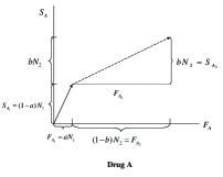
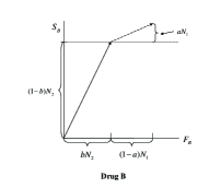
Figure 1: Simpson Paradox Prototype

This phenomenon is well-known and well-documented [5] [6] [7] [8] [9] [10] – but hope springs eternal. Only recently [1], a drug manufacturer, whose current potential blockbuster drug (Xinlay) failed to better a placebo in two clinical trials with uncorrelated protocols, proposed to a regulatory agency to pool the two sequences. If accepted, their drug would then outperform the placebo, allowing them to move forward. The regulatory agency panel was not unaware of the forced paradox, and denied the reinterpretation of the data.

2 Inverse Simpson

The Simpson Paradox is data-driven. As in (1.1), it may, or may not, hold in a given situation. However, what we may term inverse Simpson paradox is a different story: can we take a long pair of data streams – say successes and failures with drug $A$, and similarly with drug $B$ – and decompose them into two pairs of subsequences, each of which reverses the conclusion of the original pair? This can be carried out in different ways and for different purposes,

1. Most directly and legitimately, it may be realized that data from two sources were combined for simplicity, and so there is a unique decomposition called for, which may indeed reverse the conclusion. This appears to be the case in the oft-quoted Berkeley sex discrimination controversy [5].

2. Least directly and least legitimately – but perhaps an effective strategy in litigation – one can ask for that decomposition that maximally reverses the conclusion, and then use ingenuity to characterize the subsets thus obtained.

3. Putting a different spin on b), one can ask for that decomposition that maximally comes jointly to either conclusion, and use this as an investigative tool to recognize a hidden characterization of significant subsets of related entities.

At first blush, inverse Simpson, in contexts b) and c), is trivially accomplished. Fig. 2 illustrates the principle.

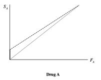
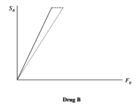
Figure 2: Inverse Simpson Prototype

The dotted lines refer to the assertedly pooled data, clearly indicating that $A$ loses to $B$. The hypothetical trial 1 data is represented by solid lines, and since $A$ has only successes, it is surely superior. And the dashed lines refer to trial 2, in which $B$ has only failures, and so surely loses.

But Fig. 2 is a suspiciously extreme version of a strategy that can be made to look more reasonable. To put it in context, let us consider the well-known Berkeley sex discrimination case [5], which we will paraphrase for numerical simplicity. The original data is that in one division, $S_{A}=41$ out of $N_{A}=100$ male applicants were admitted, a success rate of $P_{A}=.41$. On the other hand, $S_{B}=29$ of $N_{B}=100$ female applicants were admitted, a success rate of only $P_{B}=.29$. Clearly, it would seem that the admission process discriminated against females. This was not the case. In fact,

Table 2: Simplified Berkeley Admission Data

	Dept. 1	Dept. 2
Male Applicants	30	70
Males Admitted	6	35
Female Applicants	70	30
Females Admitted	14	15
Total Male Admissions/Applicants 41/100=.41
Total Female Admissions/Applicants 29/100=.29

Table 2, Simplified Berkeley Admission Data, was arrived at by combining that of two departments, say 1 and 2. Referring to Table 2, we see that the success rates of males in the two departments were $P_{A1}=.2$, $P_{A2}=.5$, with the corresponding female success rates of $P_{B1}=.2$, $P_{B2}=.5$. There was no demonstrable discrimination in either department, but “mixing watermelons and monkey wrenches” created very much of a statistical artifact.

Let us proceed to a general situation. We are given $N_{A}$ and $P_{A}=S_{A}/N_{A},\,N_{B}$, and $P_{B}=S_{B}/N_{B}$ for which, without loss of generality, $P_{A}>P_{B}$. We then imagine compartmentalizing the $A$-pool as $N_{A1}=\alpha N_{A}$, $N_{A2}=(1-\alpha)N_{A}$, and the $B$-pool as $N_{B1}=\beta N_{B}$, $N_{B2}=(1-\beta)N_{B}$; the success rates are to be given via $S_{A1}=P_{A1}N_{A1}$, $S_{A2}=P_{A2}N_{A2}$, $S_{B1}=P_{B1}N_{B1}$, $S_{B2}=P_{B2}N_{B2}$. The question then is whether $\alpha$ and $\beta$ can be chosen so that

$$P_{A1} =\lambda=P_{B1}$$ (2.1)

$$P_{A2} =\mu=P_{B2},$$

indicating no advantage to $A$ or $B$ in either case. This is trivial. Since $S_{A1}=\alpha\lambda N_{A}$, $S_{A2}=(1-\alpha)\mu N_{A}$, $S_{B1}=\beta\lambda N_{B}$, $S_{B2}=(1-\beta)\mu N_{B}$, we must have

$$P_{A} =\alpha\lambda+(1-\alpha)\mu$$ (2.2)

$$P_{B} =\beta\lambda+(1-\beta)\mu$$

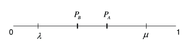
Figure 3: Placement of Averaging Parameters $\lambda$ and $\mu$

Thus, $P_{A}$ and $P_{B}$ are both averages of $\lambda$ and $\mu$, which therefore must lie outside the interval $(P_{B},\,P_{A})$ as in Fig. 3. Explicitly, of course, we have

$$\alpha =\frac{\mu-P_{A}}{\mu-\lambda} \beta =\frac{\mu-P_{B}}{\mu-\lambda}$$ (2.3)

$$1-\alpha =\frac{P_{A}-\lambda}{\mu-\lambda} 1-\beta =\frac{P_{B}-\lambda}{\mu-\lambda}$$

In situations not as clear cut as the Berkeley case, we would want to invent a hypothetical decomposition in which e.g. $\lambda$ is roughly in the middle of the $(0,\,P_{B})$ interval, $\mu$ roughly in the middle of $(P_{A},1)$, in order to allay suspicion. In the Berkeley case, we see that $\lambda=.2$, $\mu=.5$ do satisfy this criterion.

With (2.3), we find that a suitable decomposition removes the apparent bias against females: no assertion can then be made. But Fig. 2 illustrates a proactive strategy, in which a suitable decomposition reverses the original assertion and appears to establish the superiority of $A$. What is wrong with the construction of Fig. 2, aside from its suspicious extreme nature? Nothing, but the conclusion is questionable because we have not attended to the statistical significance of the new assertions, a point that was emphasized by the FDA panel cited above. Doing so forms the substance of our ensuing discussion.

3 Statistical Significance

A prototypical situation calling for statistical assessment is this. A sequence of $N$ independent Bernoulli trials – successes or failures – is carried out on the same object, resulting in $S$ successes. Given $\epsilon$, with what probability, or confidence, can we claim that $p$, the intrinsic success probability parameter, satisfies

$$|p-S/N|\leq\epsilon/N^{1/2}?$$ (3.1)

The standard approach is to start with the elementary result that, regarding $S$ as a random variable and defining $q\equiv 1-p$,

$$Pr( |S-Np|\leq N^{1/2}\epsilon|p)$$ (3.2)

$$=\sum_{j=[Np-N^{1/2}\epsilon]}^{[Np+N^{1/2}\epsilon]}\left(\begin{smallmatrix}{N}\\ {j}\end{smallmatrix}\right)p^{j}q^{N-j},$$

where [ ] denotes integer part. The device then is to identify (3.2), which is a probability on $S$-space, with a probability on $p$-space:

$$Pr(|p-S/N|\leq\epsilon/N^{1/2}|S)=Pr(|S-Np|\leq N^{1/2}\epsilon|p)$$ (3.3)

signifying our confidence that (3.1) holds.

The sort of information that will interest us will, however, in the context of this prototype, be more like: with what confidence, based upon the observed value of $S$, can we claim that

$$p\geq 1/2?$$ (3.4)

Now, the above recipe is not readily applicable, since we are no longer questioning a relationship between $p$ and $S$ that makes possible the sub rosa journey from $S$-space to $p$-space. But this is indeed the province of the Bayes approach [4] which – ignoring the controversy that continues to swirl around it – is what we will use. First of all, let up recall what (3.1) would become in a Bayesian context: we imagine joint $(p,S)$-space and quote the obvious

$$Pr(p=p^{\prime}|S=S^{\prime}) =Pr(S=S^{\prime}|p=p^{\prime})\,f(p^{\prime})/Z$$ (3.5)

$$\text{where}\,Z =\int^{\prime}_{0}Pr(S=S^{\prime}|p=p^{\prime\prime})\,f(p^{\prime\prime})dp^{\prime\prime},$$

$f$ here referring to probability density. If $f(p^{\prime})$ is the prior density on $p$-space, then

$$Pr(|p-S/N| \leq\epsilon/N^{1/2}|S=S^{\prime})$$ (3.6)

$$=\int^{S^{\prime}/N+\epsilon/N^{1/2}}_{S^{\prime}/N-\epsilon/N^{1/2}}f(p^{\prime})p^{\prime S^{\prime}}q^{\prime N-S^{\prime}}dp^{\prime}/Z$$

$$Z =\int^{\prime}_{0}f(p^{\prime})p^{\prime S^{\prime}}q^{\prime N-S^{\prime}}dp^{\prime}.$$

But suppose we choose a uniform prior, $f(p)=1$; then (3.6) becomes

$$Pr(|p-S/N|\leq\epsilon/N^{1/2})$$ (3.7)

$$=\int^{\min(S^{\prime}/N+\epsilon/N^{1/2},N)}_{\max(O,S^{\prime}/N-\epsilon/N^{1/2})}p^{\prime S}q^{\prime N-S}dp^{\prime}/Z$$

$$Z=\int^{\prime}_{0}p^{\prime S}q^{\prime N-S}dp^{\prime}=((N+1)\left(\begin{smallmatrix}{N}\\ {S}\end{smallmatrix}\right))^{-1}.$$

Eqs. (3.2, 3.3) and (3.7) are certainly not identical, but if we go to the large sample regime, i.e. the normal approximation to the binomial, then (3.2, 3.3) aver that

$$Pr(|p-S/N|\leq\epsilon/N^{1/2})=\int^{\epsilon/\sqrt{pq}}_{-\epsilon/\sqrt{pq}}e^{-\frac{1}{2}s^{\prime 2}}ds^{\prime}/\sqrt{2\pi},$$ (3.8)

which, it is easy to show is identical with the large $N$, fixed $S/N$, steepest descent expansion [3] of (3.7) around $p^{\prime}=S/N$.

On the basis of the above equivalence, we now go immediately to the question indicated by (3.4). Using Bayes with a uniform prior, precisely as in (3.7), we have

$$Pr\left(p\geq\frac{1}{2}\right)=\int^{1}_{1/2}p^{\prime S}q^{\prime N-S}dp^{\prime}/\int^{1}_{0}p^{\prime S}q^{\prime N-S}dp^{\prime}$$ (3.9)

$$=1-B_{1/2}(S+1,N+1-S)/B(S+1,N+1-S),$$

where $B$ is the Beta function, $B_{1/2}$ the corresponding incomplete Beta function [2]. Eq. (3.9) can also be written in the neat form

$$Pr\left(p\geq\frac{1}{2}\right) =1-\sum_{j=0}^{N-S}\left(\begin{smallmatrix}{N+1}\\ {j}\end{smallmatrix}\right)p^{N+1-j}q^{j}|_{p=\frac{1}{2}}$$ (3.10)

$$=1-\sum^{N-S}_{j=0}\left(\begin{smallmatrix}{N+1}\\ {j}\end{smallmatrix}\right)/2^{N+1}$$

The important point however is that this construction leads quite directly to evaluation of quantities such as $Pr(p_{A}\geq p_{B})$, that are appropriate to the Simpson paradox.

4 Level of Significance of the Inverse Paradox

The effect we are studying is not very subtle, and so it is sufficient to take a large sample limit, which strategy we adopt. However, there are several sample parameters, leading to the meaningful use of additional limiting operations. Consider first the prototype, Eq. (3.10); here,

$$\alpha_{N}(S)=\sum_{j=0}^{N-S}\left(\begin{smallmatrix}{N+1}\\ {j}\end{smallmatrix}\right)/2^{N+1}$$ (4.1)

expresses the level of significance of the assertion that $p\geq\frac{1}{2}$, and it is not until such an assessment is made that one can declare meaningful comparisons. Let us evaluate (4.1) in the large sample limit in a familiar fashion that extends at once to the question of $Pr(p_{A}\geq p_{B})$ relevant to the Simpson paradox.

Although (4.1) is finite and explicit, its implementation for large $N$ and $S$ – while trivial numerically – is a bit complex. For this purpose, the expression (3.9) is more useful; it says that

$$\alpha_{N}(S)=\int^{1/2}_{0}p^{S}(1-p)^{N-S}dp/\int^{1}_{0}p^{S}(1-p)^{N-S}dp.$$ (4.2)

By the large sample limit, we will mean that in which

$$s=N^{-1/2}\left(S-\frac{1}{2}N\right)$$ (4.3)

is fixed (to within $N^{-1/2}$) as $N\to\infty$, and we then ask for

$$\alpha(s)=\lim_{N\to\infty}\alpha_{N}(S).$$ (4.4)

This is obtained quite directly by a steepest descent evaluation [3] of (4.2). The relevant integrand is now

$$I(p)\equiv p^{S}(1-p)^{N-S}$$ (4.5)

$$=\exp\left[\left(\frac{N}{2}+N^{1/2}s\right)\,\ln\,p+\left(\frac{N}{2}-N^{1/2}s\right)\,\ln\,(1-p)\right],$$

with a maximum at

$$p_{0}=\frac{1}{2}+N^{-1/2}s,$$ (4.6)

and a corresponding expansion starting as

$$I(p)=I(p_{0})\exp-\left[\frac{N}{2}(p-p_{0})^{2}/\left(\frac{1}{4}-\frac{s^{2}}{N}\right)\right].$$ (4.7)

Hence

$$\alpha(s) =\lim_{N\to\infty}\int^{1/2}_{0}e^{-2N(p-p_{0})^{2}}dp/\int^{1}_{0}e^{-2N(p-p_{0})^{2}}dp$$ (4.8)

$$=\lim_{N\to\infty}\int^{-2s}_{-N^{1/2}-2s}e^{-x^{2}/2}dx/\int^{N^{1/2}-2s}_{-N^{1/2}-2s}e^{-x^{2}/2}dx$$

$$=\int^{-2s}_{-\infty}e^{-x^{2}/2}dx/\int^{\infty}_{-\infty}e^{-x^{2}/2}dx,$$

immediately recognizable in a normal distribution context.

We can then proceed to the desired evaluation of

$$\begin{split}Pr(p_{A}\geq p_{B}|S_{A},S_{B},N_{A},N_{B})=\\ \sideset{}{}{\iint}_{\begin{subarray}{c}1\geq p_{A}\geq p_{B}\geq 0\end{subarray}}[f(p_{A},p_{B})\,\\ Pr(S_{A},S_{B},|p_{A},p_{B},N_{A}\,N_{B})]dp_{A}\,dp_{B}/\\ \qquad\sideset{}{}{\iint}_{\begin{subarray}{c}1\geq p_{A}\geq 0\\ 1\geq p_{B}\geq 0\end{subarray}}[f(p_{A},p_{B})\\ Pr(S_{A},S_{B}|p_{A},p_{B},N_{A},N_{B})]dp_{A}\,dp_{B}.\end{split}$$ (4.9)

This is carried out in Appendix A, where we choose Bayes with uniform prior on $p_{A},p_{B}$ space and process (4.9) as we did (4.2). The result is that for large $N_{A},N_{B},$

$$\begin{split}Pr(p_{A}\geq p_{B})=\phi\left(\frac{S_{A}}{N_{A}}-\frac{S_{B}}{N_{B}}\left/\left(\frac{S_{A}(N_{A}-S_{A})}{N_{A^{3}}}\right.\right.\right.\\ \left.\left.+\frac{S_{B}(N_{B}-S_{B})}{N_{B^{3}}}\right)^{1/2}\right)\\ \text{where}\,\phi(x)=\frac{1}{\sqrt{2\pi}}\int_{-\infty}^{x}e^{-\frac{1}{2}y^{2}}dy\end{split}$$ (4.10)

Unsurprisingly, we can obtain (4.10) as well by a version of the probability space equivalence assertion employed in (3.3). It is only necessary to consider the random variable

$$\xi=\frac{S_{A}}{N_{A}}-\frac{S_{B}}{N_{B}}$$ (4.11)

where $S_{A}$ and $S_{B}$ are binomially distributed with success probabilities $p_{A}$ and $p_{B}$. Since we find at once that

$$E(e^{\gamma\left(\frac{S_{A}}{N_{A}}-\frac{S_{B}}{N_{B}}\right)})$$ (4.12)

$$=(p_{A}e^{\gamma/N_{A}}+q_{A})^{N_{A}}(p_{B}e^{-\gamma/N_{B}}+q_{B})^{N_{B}},$$

it follows directly that

$$E(\xi|p_{A},p_{B}) =p_{A}-p_{B}$$ (4.13)

$$\text{Var}(\xi|p_{A},p_{B}) =\frac{p_{A}}{N_{A}}q_{A}+\frac{p_{B}}{N_{B}}q_{B}$$

and then from the central limit theorem that in the limit $N_{A}$, $N_{B}\to\infty$,

$$Pr\left(\frac{S_{A}}{N_{A}}-\frac{S_{B}}{N_{B}}\geq p_{A}-p_{B}+\Delta|p_{A},p_{B}\right)$$ (4.14)

$$=\phi(-\Delta/(p_{A}q_{A}/N_{A}+p_{B}q_{B}/N_{B})^{1/2})$$

The same sleight of hand as in (3.3) then converts this to

$$Pr\left(p_{A}-p_{B}\leq\frac{S_{A}}{N_{A}}-\frac{S_{B}}{N_{B}}-\Delta|S_{A},S_{B}\right)$$ (4.15)

$$=\phi\left(-\Delta/\left(\frac{S_{A}(N_{A}-S_{A})}{N_{A}^{3}}+\frac{S_{B}(N_{B}-S_{B})}{N_{B}^{3}}\right)^{1/2}\right),$$

and so, setting $\Delta=\frac{S_{A}}{N_{A}}-\frac{S_{B}}{N_{B}}$, to (4.10), as was to be shown.

5 Realizations of the Inverse Paradox

Now let us make use of the result (4.10). If our initial data is characterized by $S_{A}$, $S_{B}$, $N_{A}+N_{S}=N$, and $P_{A}=S_{A}/N_{A},\,P_{B}=S_{B}/N_{B}$, then the confidence level with which we can assert that $p_{A}\geq p_{B}$ is given by

$$\phi (N^{1/2}C_{AB})$$ (5.1)

$$C_{AB} =(P_{A}-P_{B})/\sigma_{AB}>0$$

$$\sigma^{2}_{AB} =\frac{P_{A}(1-P_{A})}{N_{A}/N}+\frac{P_{B}(1-P_{B})}{N_{B}/N}.$$

Our objective is to supply a decomposition into two hypothetical trials $(S_{A1},N_{A1},\\ S_{B1},N_{B1})$ and $(S_{A2},N_{A2},S_{B2},N_{B2})$ such that

$$\text{if}\,C^{\prime}_{i} =(P_{Bi}-P_{Ai})/\sigma_{i},\quad i=1,2$$ (5.2)

$$\text{where}\,P_{Ai} =S_{Ai}/N_{Ai},\quad P_{Bi}=S_{Bi}/N_{Bi}$$

$$\sigma^{2}_{i} =\frac{P_{Ai}(1-P_{Ai})}{N_{Ai}/N}+\frac{P_{Bi}(1-P_{Bi})}{N_{Bi}/N},$$

$$\quad\text{then}\,C^{\prime}_{i}>0\,\text{for}\,i=1,2.$$

In fact, to be definite, we suppose that the two pairs of trials reverse the initial assertion at a common level of confidence

$$(P_{B1}-P_{A1})/\sigma_{1}=C^{\prime}=(P_{B2}-P_{A2})/\sigma_{2}$$ (5.3)

with $C^{\prime}>0$. To start, we need to find the restrictions on $C^{\prime}$ under which the required $(P_{A1},P_{A2},P_{B1},P_{B2})$ satisfying (5.2) can be found.

The solution is direct but algebraically cumbersome, and is presented in detail in Appendices B and C. The conclusion of the former is that if $\alpha\geq\beta$, then

$$C^{\prime}\leq\min\left(\frac{\bar{\beta}\bar{P}_{A}-\bar{\alpha}\bar{P}_{B}}{\bar{\alpha}\sigma_{B}},\frac{\bar{\beta}\bar{P}_{A}-\bar{\alpha}\bar{P}_{B}}{\bar{\beta}\sigma_{A}},\right.$$ (5.4)

$$\left.\frac{\alpha P_{B}-\beta P_{A}}{\alpha\sigma_{B}},\frac{\alpha P_{B}-\beta P_{A}}{\beta\sigma_{A}}\right).$$

Since we require $C^{\prime}\geq 0$, this implies that

$$\alpha/\beta\geq P_{A}/P_{B}\geq 1,\qquad\bar{\beta}/\bar{\alpha}\geq\bar{P}_{B}/\bar{P}_{A}\geq 1.$$ (5.5)

In (5.4) and (5.5), we uniformly adopt the notation:

$$\text{if}\,\,0\leq x\leq 1,\,\text{then}\,\,\bar{x}\equiv 1-x.$$ (5.6)

Eq. (5.4) is a bit involved and, even worse, contains the unknown parameters $p_{Ai}$, $p_{Bi}$ implicitly. But it can be simplified by reducing its right hand side and thereby strengthening the requirement on $C^{\prime}$ a bit. This is carried out in Appendix C, with the conclusion that, if $\alpha\geq\beta$, then

$$\begin{split}P_{A}+P_{B}\geq 1:C^{\prime}\leq 2(\gamma\bar{\gamma})^{1/2}((\bar{P}_{B}/\bar{P}_{A})^{2}-1)\\ (P_{A}-P_{B})(P_{B}/P_{A})/\left[\left(\frac{P_{A}}{P_{B}}\frac{\bar{P}_{B}}{\bar{P}_{A}}\right)^{2}-1\right]\\ P_{A}+P_{B}\leq 1:C^{\prime}\leq 2(\gamma\bar{\gamma})^{1/2}((P_{A}/P_{B})^{2}-1)\\ (P_{A}-P_{B})(\bar{P}_{A}/\bar{P}_{B})/\left[\left(\frac{P_{A}}{P_{B}}\frac{\bar{P}_{B}}{\bar{P}_{A}}\right)^{2}-1\right]\\ \text{where}\,\,\gamma=N_{A}/N\end{split}$$ (5.7)

are sufficient to carry out the apparent reversal of ranking of $A$ and $B$.

Let us take a simple example that has been previously quoted [4] [8]. We will paraphrase it and use rounded off data. Hospitals $A$ and $B$ specialize in treating a certain deadly disease. $N_{A}=1000$ patients are treated at $A$ and $N_{B}=1000$ at $B$. Of these, $S_{A}=900$ recover, while $S_{B}=800$ recover, so that $P_{A}=.9$, $P_{B}=.8$ and Hospital $A$ is apparently the place to go. In fact, one computes $C_{AB}=.05$, so that this conclusion is supported at the $.05\times(2000)^{1/2}=2.24$ standard deviation level. Detailed investigation shows that matters are not so simple. Some patients enter in otherwise good shape, others in poor shape. Of the former, $N_{A1}=900$ enter hospital $A$, and 870 recover; of the latter, $N_{A2}=100$ enter and 30 recover, so $P_{A1}=.967$, $P_{A2}=.3$.

Table 3: Simplified Hospital Recovery Data

	Good Shape	Poor Shape
Admissions to Hospital A	900	100
Recovered in Hospital A	870	30
Admissions to Hospital B	600	400
Recovered in Hospital B	590	210
Total Recovered/Admissions in A: 900/1000=.9
Total Recovered/Admissions in B: 800/1000=.8

On the other hand, $N_{B1}=600$ enter Hospital $B$ in good shape and $S_{B1}=590$ recover, whereas $N_{B2}=400$, $S_{B2}=210$. Thus, $P_{B1}=.983$, $P_{B2}=.55$. We see that by not mixing the two classes of patients, Hospital $B$ is superior for each class – at levels $C^{\prime}_{1}=.038$ (1.7 standard deviations) and $C^{\prime}_{2}=.176$ (7.9 standard deviations). Simpson, or inverse Simpson, depending upon one’s point of view, is certainly exemplified.

Of course, the criteria as to which patients entered in good shape, which in poor shape, are a bit fuzzy. Given the aggregate data, the decomposition into the two classes could, as we have seen, been planned with the intention of most convincingly asserting the opposite of the conclusion from the aggregate data. If this had been done according to the prescription of (5.7), then with the same input data, we would have found $\alpha=.935$, $\beta=.738$ (not far from the $\alpha=.9$, $\beta=.6$ corresponding to the additional data presented) and concluded with the superiority of Hospital $B$ at a confidence level corresponding to $C^{\prime}\leq.107$ or 4.79 standard deviations for each class of patients.

6 Concluding Remarks

The Simpson paradox, one of the simplest examples of the common misuse of statistics (think meta-analysis?) has received increasing attention, since the consequences of its use – or misuse – can be quite severe (as well as profitable). In the classical Simpson Paradox, the only question is whether or not to combine data from different sources (and trying to justify the decision to combine). What we have seen here is that the inverse Simpson paradox, even in its most “sophisticated” version in which mean differences are weighted by appropriate standard deviations, is nearly universally applicable. This can be an effective analytical tool, but can equally well be an effective technique for distorting statistical data.

Appendix A Evaluation of (4.9)

Choosing Bayes with a uniform prior on $p_{A},p_{B}$ space, (4.9) becomes

$$\begin{split}\sideset{}{}{\iint}_{\begin{subarray}{c}1\geq p_{A}\geq p_{B}\geq 0\end{subarray}}Pr\left(S_{A},S_{B}|p_{A},p_{B},N_{A},N_{B}\right)dp_{A}\,dp_{B}\left/\right.\\ \sideset{}{}{\iint}_{\begin{subarray}{c}1\geq p_{A},p_{B}\geq 0\end{subarray}}Pr\left(S_{A},S_{B}|p_{A},p_{B},N_{A},N_{B}\right)dp_{A}\,dp_{B}\\ =\sideset{}{}{\iint}_{\begin{subarray}{c}1\geq p_{A}\geq p_{B}\geq 0\end{subarray}}p_{A}^{S_{A}}\,p_{B}^{S_{B}}\,q_{A}^{F_{A}}\,q_{B}^{F_{B}}\,dp_{A}\,dp_{B}\left/\right.\\ \sideset{}{}{\iint}_{\begin{subarray}{c}1\geq p_{A},p_{B}\geq 0\end{subarray}}p_{A}^{S_{A}}\,p_{B}^{S_{B}}\,q_{A}^{F_{A}}\,q_{B}^{F_{B}}\,dp_{A}\,dp_{B}\\ =\int^{1}_{0}\left(\int_{0}^{p_{A}}p_{B}^{S_{B}}q_{B}^{F_{B}}dp_{B}\right)p_{A}^{S_{A}}q_{A}^{F_{A}}dp_{A}\left/\right.\\ \int^{1}_{0}\!\int p_{B}^{S_{B}}\,q_{B}^{F_{B}}\,p_{A}^{S_{A}}\,q_{A}^{F_{A}}\,dp_{B}\,dp_{A}\\ =\int^{1}_{0}B_{p_{A}}\left(S_{A}+1,F_{B}+1\right)p_{A}^{S_{A}}\,q_{A}^{F_{A}}\,dp_{A}/\\ B\left(S_{B}+1,F_{B}+1\right)B\left(S_{A}+1,F_{A}+1\right).\end{split}$$ (A.1)

Applying the known expansion of the incomplete Beta function [2], this reduces after a little algebra to

$$Pr(p_{A} \geq p_{B}|S_{A},S_{B},N_{A},N_{B})$$ (A.2)

$$=\sum^{F_{A}+F_{B}}_{j=0}\left(\begin{smallmatrix}{S_{A}+S_{B}+1+j}\\ {S_{A}}\end{smallmatrix}\right)\left(\begin{smallmatrix}{F_{A}+F_{B}-j}\\ {F_{A}}\end{smallmatrix}\right)$$

$$/\left(\begin{smallmatrix}{N_{A}+N_{B}+2}\\ {N_{A}+1}\end{smallmatrix}\right),$$

or introducing $S=S_{A}+S_{B}$, $N=N_{A}+N_{B}$ for notational convenience,

$$Pr(p_{A} \geq p_{B}|S_{A},S_{B},N_{A},N_{B})$$ (A.3)

$$=\sum^{F}_{j=0}\left(\begin{smallmatrix}{S+1+j}\\ {S_{A}}\end{smallmatrix}\right)\left(\begin{smallmatrix}{F-j}\\ {F_{A}}\end{smallmatrix}\right)/\left(\begin{smallmatrix}{N+2}\\ {N_{A}+1}\end{smallmatrix}\right)$$

But we will go to the large sample limit defined by fixed

$$s=N_{A}^{-1/2}\left(S_{A}-\frac{1}{2}N_{A}\right), \gamma=N_{A}/N,$$ (A.4)

$$s^{\prime}=N_{B}^{-1/2}\left(S_{B}-\frac{1}{2}N_{B}\right) 1-\gamma\equiv N_{B}/N$$

as $N\to\infty$. We could proceed precisely as in (4.5 – 4.8), but if we imagine a large sample limit from the outset, the derivation is brief and standard. Consider drug $A$. A uniform prior for $p_{A}$ is given by the beta distribution

$$f(p_{A}) =b(1,1;p_{A})$$ (A.5)

$$\text{where}\,b(m,n;p_{A}) =p_{A}^{m-1}q_{A}^{n-1}/B(m,n)$$

$$B(m_{1}n) =m-1!n-1!/m+n-1!$$

which, after$S_{A}$ successes in $N_{A}$ trials creates the posterior distribution

$$b(1+S_{A},1+N_{A}-S_{A};p_{A}).$$ (A.6)

Drug B works the same way. It follows that

$$E(p_{A}-p_{B}) =\frac{S_{A}+1}{N_{A}+1}-\frac{S_{B}+1}{N_{B}+1}$$ (A.7)

$$\text{Var}(p_{A}-p_{B}) =\frac{(S_{A}+1)(N_{A}+1-S_{A})}{(N_{A}+1)^{2}(N_{A}+2)}$$

$$+\frac{(S_{B}+1)(N_{B}+1-S_{B})}{(N_{B}+1)^{2}(N_{B}+2)},$$

and so by the central limit theorem for large $N_{A}$, $N_{B}$,

$$Pr(p_{A}\geq p_{B})=\phi\left(\frac{S_{A}}{N_{A}}-\frac{S_{B}}{N_{B}}/\left(\frac{S_{A}(N_{A}-S_{A})}{N_{A}^{3}}\right.\right.$$ (A.8)

$$\left.\left.+\frac{S_{B}(N_{B}-S_{B})}{N_{B}^{3}}\right)^{1/2}\right)$$

$$\text{where}\,\phi(x)=\frac{1}{\sqrt{2\pi}}\int_{-\infty}^{x}e^{-\frac{1}{2}y^{2}}dy.$$

Appendix B Restrictions on $C^{\prime}$

Eq. (5.3) itself imposes two conditions. Aside from the crucial $0\leq P_{A1},P_{A2},\\ P_{B1},P_{B2}\leq 1$, there are just two more due to the composition conditions that $S_{A1}+S_{A2}=S_{A},\,N_{A1}+N_{A2}=N_{A},\,S_{B1}+S_{B2}=S_{B},\,N_{B1}+N_{B2}=N_{B}$. We reintroduce the notation of Section 2:

$$N_{A1}=\alpha N_{A}, \qquad N_{B1}=\beta N_{B}$$ (B.1)

and hereafter uniformly adopt the notation that

$$\text{if}\,\,0\leq x\leq 1,\qquad\text{then}\,\,\bar{x}\equiv 1-x.$$ (B.2)

Thus $S_{A1}+S_{A2}=S_{A}$ implies $P_{A1}N_{A1}+P_{A2}N_{A2}=P_{A}N_{A}$, or

$$\alpha P_{A1}+\bar{\alpha}P_{A2}=P_{A}$$ (B.3)

and similarly

$$\beta P_{B1}+\bar{\beta}P_{B2}=P_{B}.$$ (B.4)

We also append (5.3) in the form

$$P_{B1}-P_{A1} =C^{\prime}\sigma_{1}$$ (B.5)

$$P_{B2}-P_{A2} =C^{\prime}\sigma_{2},$$

and solve (B.3), (B.4), (B.5) to yield

$$P_{A1} =K_{1}+\frac{\bar{\alpha}}{\alpha-\beta}\,C^{\prime}\sigma_{B}, P_{A2} =K_{2}-\frac{\alpha}{\alpha-\beta}\,C^{\prime}\sigma_{B},$$ (B.6)

$$P_{B1} =K_{1}+\frac{\bar{\beta}}{\alpha-\beta}\,C^{\prime}\sigma_{\alpha}, P_{B2} =K_{2}-\frac{\beta}{\alpha-\beta}\,C^{\prime}\sigma_{\alpha}$$

where

$$K_{1} =(\bar{\beta}P_{A}-\bar{\alpha}P_{B})/(\alpha-\beta), \,\,\sigma_{\alpha} =\alpha\sigma_{1}+\bar{\alpha}\sigma_{2},$$ (B.7)

$$K_{2} =(\alpha P_{B}-\beta P_{A})/(\alpha-\beta), \,\,\sigma_{\beta} =\beta\sigma_{1}+\bar{\beta}\sigma_{2}.$$

Eqs. (B.6), (B.7) are realizable if the requirements $0\leq P_{A1},P_{A2},P_{B1},P_{B2}\leq 1$ are satisfied. Since we are asserting, without loss of generality, that $p_{A}\geq p_{B}$, we of course have the condition

$$P_{A}\geq P_{B},\bar{P}_{B}\geq\bar{P}_{A}.$$ (B.8)

There are then two cases to consider. If $\alpha\geq\beta$, it is easily seen that $K_{1}\geq 0$, $K_{2}\leq 1$, so that $P_{A1},P_{B1}\geq 0$, $P_{A2},P_{B2}\leq 1$ are already satisfied. The remaining four conditions $P_{A1},P_{B1}\leq 1$, $P_{A2},P_{B2}\geq 0$ can then be gathered together as

$$\text{if}\,\alpha\geq\beta\,\text{then}$$ (B.9)

$$C^{\prime}\leq\min\left(\frac{(\alpha-\beta)(1-K_{1})}{\bar{\alpha}\sigma_{\beta}},\frac{(\alpha-\beta)(1-K_{1})}{\bar{\beta}\sigma_{\alpha}},\right.$$

$$\left.\frac{(\alpha-\beta)K_{2}}{\alpha\sigma_{\beta}},\frac{(\alpha-\beta)K_{2}}{\beta\sigma_{\alpha}}\right),$$

or, inserting (B.7),

$$C^{\prime}=\min\left(\frac{\bar{\beta}\bar{P_{A}}-\bar{\alpha}\bar{P_{B}}}{\bar{\alpha}\sigma_{\beta}},\frac{\bar{\beta}\bar{P_{A}}-\bar{\alpha}\bar{P_{B}}}{\bar{\beta}\sigma_{\alpha}},\right.$$ (B.10)

$$\left.\frac{\alpha P_{B}-\beta P_{A}}{\alpha\sigma_{\beta}},\frac{\alpha P_{B}-\beta P_{A}}{\beta\sigma_{\alpha}}\right).$$

Similarly,

$$\text{if}\,\alpha\leq\beta\,\text{then}$$ (B.11)

$$C^{\prime}\leq\min\left(\frac{\bar{\alpha}P_{B}-\bar{\beta}P_{A}}{\bar{\alpha}\sigma_{\beta}},\frac{\bar{\alpha}P_{B}-\bar{\beta}P_{A}}{\bar{\beta}\sigma_{\alpha}},\right.$$

$$\left.\frac{\beta\bar{P_{A}}-\alpha\bar{P_{B}}}{\alpha\sigma_{\beta}},\frac{\beta\bar{P_{A}}-\alpha\bar{P_{B}}}{\beta\sigma_{\alpha}}\right)$$

Since we require $C^{\prime}\geq 0$, immediate consequences are that

$$\text{if}\,\,\alpha\geq\beta,\text{then}\,\,\frac{\alpha}{\beta}\geq\frac{P_{A}}{P_{B}}\geq 1,\qquad\frac{\bar{\beta}}{\bar{\alpha}}\geq\frac{\bar{P_{B}}}{\bar{P_{A}}}\geq 1$$ (B.12)

$$\text{if}\,\,\alpha\leq\beta,\,\,\frac{\bar{\alpha}}{\bar{\beta}}\geq\frac{P_{A}}{P_{B}}\geq 1,\,\,\frac{\beta}{\alpha}\geq\frac{\bar{P_{B}}}{\bar{P_{A}}}\geq 1$$

must hold.

Appendix C Simplification of (5.4)

The major step is the observation, from (5.2) that

$$\sigma^{2}_{i}\leq\frac{N}{4}\left(\frac{1}{N_{Ai}}+\frac{1}{N_{Bi}}\right),$$ (C.1)

so that

$$\sigma^{2}_{1} \leq\frac{N}{4}\left(\frac{1}{\alpha N_{A}}+\frac{1}{\beta N_{B}}\right)$$ (C.2)

$$\sigma^{2}_{2} \leq\frac{N}{4}\left(\frac{1}{\bar{\alpha}N_{A}}+\frac{1}{\bar{\beta}N_{B}}\right)$$

Hence,

$$\text{if}\,\alpha\geq\beta,\qquad\sigma^{2}_{1} \leq\frac{1}{4\beta}\left(\frac{N}{N_{A}}+\frac{N}{N_{B}}\right)$$ (C.3)

$$\qquad\sigma^{2}_{2} \leq\frac{1}{4\bar{\alpha}}\left(\frac{N}{N_{A}}+\frac{N}{N_{B}}\right),$$

yielding

$$\begin{matrix}\sigma_{2}\\ \sigma_{B}\end{matrix}\}\leq\max(\sigma_{1},\sigma_{2})\leq\frac{1}{2}\left(\frac{N}{N_{A}}+\frac{N}{N_{B}}\right)^{1/2}$$ (C.4)

$$\max\left(\frac{1}{\beta^{1/2}},\frac{1}{\bar{\alpha}^{1/2}}\right).$$

Setting $N_{A}/N=\gamma$, condition (5.4) can therefore be strengthened to

$$\alpha\geq\beta:C^{\prime}\leq 2(\gamma\bar{\gamma})^{1/2}\min(\beta,\bar{\alpha})^{1/2}$$ (C.5)

$$\min\left[\frac{1}{\bar{\beta}}(\bar{\beta}\bar{P_{A}})-\bar{\alpha}\bar{P_{B}}),\frac{1}{\alpha}(\alpha P_{B}-\beta P_{A})\right].$$

And in the same way, we obtain the strengthened

$$\alpha\leq B:C^{\prime}\leq 2(\gamma\bar{\gamma})^{1/2}\min(\alpha,\bar{\beta})^{1/2}$$ (C.6)

$$\min\left[\frac{1}{\bar{\alpha}}(\bar{\alpha}P_{B}-\bar{\beta}P_{A}),\frac{1}{\beta}(\beta\bar{P}_{A}-\alpha\bar{P}_{B})\right].$$

Eqs. (C.5) and (C.6) are valid for all $\alpha,\beta$, and we may indeed find the largest feasible range for $C^{\prime}$ by maximizing their right hand sides over $\alpha$ and $\beta$. Again, to reduce complexity, let us take the special case in which:

$$\alpha\geq\beta:\bar{\alpha}/\bar{\beta}=(\bar{P_{A}}/\bar{P_{B}})^{2},\beta/\alpha=(P_{B}/P_{A})^{2}$$ (C.7)

so that

$$\alpha=[(P_{A}/P_{B})^{2}(\bar{P_{B}}/\bar{P_{A}})^{2}-(P_{A}/P_{B})^{2}]/$$ (C.8)

$$[(P_{A}/P_{B})^{2}(\bar{P_{B}}/\bar{P_{A}})^{2}-1]$$

$$\beta=[(\bar{P_{B}}/\bar{P_{A}})^{2}-1]/[(P_{A}/P_{B})^{2}(\bar{P_{B}}/\bar{P_{A}})^{2}-1]$$

converting (C.5) and (C.6) to

$$\begin{split}\alpha\geq\beta:C^{\prime}\leq 2(\gamma\bar{\gamma})^{1/2}/[(P_{A}/P_{B})^{2}(\bar{P_{B}}/\bar{P_{A}})^{2}-1]\\ \min[(\bar{P_{B}}/\bar{P_{A}})^{2}-1,(P_{A}/P_{B})^{2}-1]\\ \cdot\min(\bar{P_{A}}-\bar{P_{A}}^{2}/\bar{P_{B}},P_{B}-P_{B}^{2}/P_{A}).\end{split}$$ (C.9)

But $(\bar{P_{A}}-\bar{P_{A}}^{2}/\bar{P_{B}})-(P_{B}-P_{B}^{2}/P_{A})=(1-P_{A}-P_{B})(P_{A}+P_{B})^{2}/P_{A}\bar{P_{B}}$ and $((\bar{P_{B}}/\bar{P_{A}})^{2}-1)-((P_{A}/P_{B})^{2}-1)=(P_{A}+P_{B}-1)\frac{P_{A}-P_{B}}{P_{A}\bar{P_{B}}}\left(\frac{P_{A}}{P_{B}}+\frac{\bar{P_{B}}}{\bar{P_{A}}}\right)$, so it follows that in the $\alpha\geq\beta$ case,

$$P_{A}+P_{B}\geq 1:C^{\prime}\leq 2(\gamma\bar{\gamma})^{1/2}\left(\left(\frac{\bar{P_{B}}}{\bar{P_{A}}}\right)^{2}-1\right)$$ (C.10)

$$(P_{A}-P_{B})\frac{P_{B}}{P_{A}}/\left[\left(\frac{P_{A}}{P_{B}}\frac{\bar{P_{B}}}{\bar{P_{A}}}\right)^{2}-1\right]$$

$$P_{A}+P_{B}\leq 1:C^{\prime}\leq 2(\gamma\bar{\gamma})^{1/2}\left(\left(\frac{P_{A}}{P_{B}}\right)^{2}-1\right)$$

$$(P_{A}-P_{B})\frac{\bar{P_{A}}}{\bar{P_{B}}}/\left[\left(\frac{P_{A}}{P_{B}}\frac{\bar{P_{B}}}{\bar{P_{A}}}\right)^{2}-1\right]$$

are sufficient to carry out the apparent reversal of ranking of $A$ and $B$. The decomposition corresponding to the choice $\alpha\leq\beta$ can of course be similarly specialized.

References

[1]Abboud, L. (2005). Abbott Seeks to Clear Stalled Drug. Wall Street Journal, Sept. 12.
[2]Abramowitz, M. and Stegun, I. A. (1965). Handbook of
Mathematical Functions, Dover Publications, New York.
[3]Beckenbach, E. F., editor, (1956). Modern Mathematics for
the Engineer, McGraw-Hill, New York, Chapter 18.
[4]Berger, J. O. (1985). Statistical Theorey and Bayesian
Analysis. Statistical Decision Theory and Bayesian Analysis. Springer-Verlag, New York.
[5]Bickel, P. J., Hammel, E. A., and O’Connell, J. W. (1975). Sex
Bias in Graduate Admissions: Data from Berkeley. Science187, 398 – 404.
[6]Capocci, A. and Calaion, F. (2006). Mixing properties of
growing networks and Simpson’s Paradox. Phys. Rev.E74
026122.
[7]Moore, D. S. and McCabe, G. P. (1998). Introduction to
the Practice of Statistics, 100 – 201. W. Freeman and Co., New
York.
[8]Moore, T. Simpson and Simpson-like Paradox Examples. see
www.math.grinnell.edu/mooret/reports/SimpsonExamples.pdf
[9]Saari, D. (2001). Decisions and Elections, Cambridge
University Press, Cambridge.
[10]Simpson, E. H. (1951). The interpretation of interaction in
Contingency Tables. J. Roy. Stat. Soc.B13, 238 – 241.